


Abstract
Satellite-based inverse modeling has the potential to drive aerosol precursor emissions, but its efficacy for improving chemistry transport models (CTMs) remains elusive because of its likely inherent dependence on the error characteristics of a specific CTM used for the inversion. This issue is quantitively assessed here by using three CTMs. We show that SO2 emissions from global GEOS-Chem adjoint model and OMI SO2 data, when combined with spatial variation of bottom-up emissions, can largely improve WRF-Chem and WRF-CMAQ forecast of SO2 and aerosol optical depth (in reference to moderate resolution imaging spectroradiometer data) in China. This suggests that the efficacy of satellite-based inversion of SO2 emission appears to be high for CTMs that use similar or identical emission inventories. With the advent of geostationary air quality monitoring satellites in next 3 years, this study argues that an era of using top-down approach to rapidly update emission is emerging for regional air quality forecast, especially over Asia having highly varying emissions.
Export citation and abstract BibTeX RIS

Original content from this work may be used under the terms of the Creative Commons Attribution 4.0 license. Any further distribution of this work must maintain attribution to the author(s) and the title of the work, journal citation and DOI.
1. Introduction
SO2 is considered as an important air pollutant, which is released into the above-canopy atmosphere from anthropogenic sources (coal-fired energy generations, industries, transports, and residential activities) and natural processes (volcanoes). Ambient SO2 could be oxidized via gas-phase oxidation by OH radicals, as well as aqueous-phase reaction with H2O2 and O3, and via heterogeneous process involving NO2 (Cheng et al 2016), forming H2SO4 and further sulfate aerosol. SO2 and its products have adverse effects on air quality and visibility, and also affect global climate by scattering solar radiation and changing cloud properties.
Recent estimations of SO2 emission span several folds of magnitude among different studies. The conventional method, bottom-up approach, is based on activity statistics and emission factors to quantify the emission. However, although much progress has been made (Streets et al 2003, Zhang et al 2009, Li et al 2017), bottom-up results are often outdated with a time lag of 1–2 years, mainly due to the lack of accurate and timely statistics. The time lag of bottom-up emission can be problematic for regional air quality modeling in the events that lead to the large change of emissions (such as the COVID-19 pandemic). Satellite remote sensing, from a top-down perspective, is being considered as a useful tool to identify sources and to update the bottom-up emissions, in terms of both magnitude and timeliness (Wang et al 2012, 2015, 2020a, 2020b, Xu et al 2013, Fioletov et al 2015, 2016, Liu et al 2018). Koukouli et al (2018) used CHIMERE model and 10 years of O3 monitoring instrument (OMI)/Aura total SO2 columns to update the pre-existing Multiresolution Emission Inventory for China (MEIC), and complemented it with several new sources in southwest and northeast of China into the posterior inventory. Wang et al (2016b) developed a method that used OMI SO2 observations and the GEOS-Chem adjoint model for timely updates to anthropogenic SO2 emissions. They captured a 20% reduction of anthropogenic emissions occurred in Beijing and its surrounding regions in August 2008 due to the Olympic Games as compared to April 2008.
However, top-down analyses implicitly assume that the relationship between the emission and atmospheric abundances is well captured by the inverse models, thus, all the biases between the model and the observations are mostly due to the inaccuracy of emission inventories. Because of this inherent assumption, a question arises: can the top-down estimate of emission be useful to improve those regional chemistry transport models (CTM) that are not used in the top-down inversion? This question is not quantitively and formally addressed in the literature although Miyazaki et al (2020) found that the ensemble Kalman filter approach using four global models as ensemble members can lead to overall improvements of simulation of ensemble member, implying (implicitly) the possibility of common emission errors among different models. This question is addressed for the first time here by using three different models: one is used in updating bottom-up emission to form top-down emission estimates, and the other two independently for evaluating the top-down emission. By doing so, the efficacy of the top-down approach can be fully evaluated, especially regarding its dependence on the host CTM that is used as the basis for inversion. To implement this approach (whose conceptual schema shown in figure S1 (available online at stacks.iop.org/ERL/16/035018/mmedia)), we first used the global CTM, the GEOS-Chem adjoint model and OMI SO2 slant column densities (SCDs) to obtain top-down SO2 inventory of China, largely following the work by Wang et al (2016b). The other two CTMs, regional WRF-Chem and CMAQ, with completely different physics and chemistry schemes, are used to evaluate top-down SO2 emission, by comparing their simulations with in situ surface SO2 measurements, moderate resolution imaging spectroradiometer (MODIS) aerosol optical depth (AOD), as well as OMI SO2 vertical column densities (VCDs). This study differs from the past studies in that: (a) we present a new method to evaluate the efficacy of the top-down emission, for the first time, by using three models with different chemistry parameterization, spatial resolution and interaction of meteorological process, and (b) we test this method by 4 month-long simulations representing four seasons, and evaluate the results using multiple observations.
2. Method and data
2.1. The WRF-Chem and CMAQ models
We employed two regional CTMs, WRF-Chem (v3.9.1) and CMAQ (v5.0.2), to simulate SO2 and sulfate particle in China for the year 2009. In the WRF-Chem simulations, we conducted three sets of different chemical mechanisms for gas-phase chemistry and aerosol formation as follows: (a) RADM2 coupled with SORGAM, (b) SAPRC99 coupled with eight-bin MOSAIC, and (c) the same as (b) but adding extra heterogeneous formation of sulfate following the parameterization following Ma et al (2020) and Wang et al (2016a). The wet deposition process and related aqueous-phase chemistry were based on Easter et al (2004) and Zaveri et al (2005). WRF-Chem considered the interaction between meteorology and chemistry. In CMAQ simulations, we employed SAPRC11 to treat gas-phase chemical transformation and AERO6 to represent aerosol reaction. The wet deposition and aqueous-phase chemistry in CMAQ were based on Foley et al (2010). Details of the model scenarios can be found in table 1. WRF-Chem, CMAQ, and GEOS-Chem have large differences in physical and chemical schemes, and for details please refers to table S1.
Table 1. List of chemical models and mechanisms used in this study.
| Model | Mechanism | |
|---|---|---|
| Model 1 | WRF-Chem | RADM2 + SORGAM |
| Model 2 | WRF-Chem | SAPRC99 + MOSAIC |
| Model 3 | WRF-Chem | SAPRC99 + MOSAIC + heterogeneous sulfate |
| Model 4 | WRF-CMAQ | SRARC11 + AERO6 |
We simulated a 280 × 160 girds region covering China with a horizontal resolution of 0.25 degree (figure S2) for WRF-Chem, and a 190 × 120 grids region with a horizontal resolution of 36 km for CMAQ. Vertical layers in both CTMs extended from the surface up to 50 hPa with seven layers below 1 km to emphasize boundary layer processes. Initial and boundary conditions of meteorological fields were taken from NCEP FNL operational global analysis data, and initial and boundary conditions of chemistry were derived by a global chemical transport model (model for o3 and related chemical tracers, MOZART) (Emmons et al 2010). Each simulation was conducted for 4 months (January, April, July, and October) to represent the typical meteorological and emission conditions for the each of the four seasons in 2009. Each month-long simulation was initialized for the last 6 days of the previous month.
2.2. MEIC SO2 emissions
In this study, under each model scenario, we further conducted two comparative simulations to evaluate the model performances of different SO2 emissions in China. The first was the so-called the prior run in which the anthropogenic SO2 emission inventory was taken from the MEIC inventory (Li et al 2017). This MEIC emission estimates also include other gaseous and particulate pollutants (NOx , VOCs, CO, NH3, PM2.5 and PM10) for the year of 2009, with a native resolution of 0.25°. The MEIC emissions sources consists various sectors such as industry, power, residential, transportation and agriculture, and the emission estimates are based on a collection of statistics and newly developed emission factors. The MEIC inventory estimate anthropogenic SO2 emission of 28.6 Tg yr−1 in total over China in 2009. Table 2 shows the specific SO2 emissions in different regions and different seasons, and figures 1(a) and S3 show their spatial distributions. Anthropogenic SO2 emissions were mostly concentrated in Central China (28%), the North China Plain (NCP) (23%), and the Sichuan basin (10%), with seasonal variability less than ±14%.

Figure 1. Prior and posterior anthropogenic SO2 emissions in China for 2009. Regional emission totals are shown inset in red, (c) shows the differences between prior and posterior emissions, (d) shows ratios of the differences, for the girds where the differences are larger than 0.1 Gg yr−1.
Download figure:
Standard image High-resolution imageTable 2. Anthropogenic SO2 emissions in China in 2009. The prior emission is from MEIC emission inventory, and the posterior emission is the satellite-constrained SO2 emission using GEOS-Chem adjoint model.
| Region | January (Tg mon−1) | April (Tg mon−1) | July (Tg mon−1) | October (Tg mon−1) | Annual (Tg yr−1) |
|---|---|---|---|---|---|
| Prior | |||||
| Central China | 0.74 | 0.64 | 0.68 | 0.63 | 8.08 |
| North China Plain | 0.61 | 0.54 | 0.56 | 0.51 | 6.65 |
| Southwest | 0.30 | 0.25 | 0.21 | 0.22 | 2.92 |
| Sichuan basin | 0.27 | 0.23 | 0.22 | 0.21 | 2.81 |
| Northwest | 0.23 | 0.20 | 0.20 | 0.19 | 2.45 |
| Yangtze River Delta | 0.20 | 0.20 | 0.21 | 0.19 | 2.40 |
| Northeast | 0.16 | 0.14 | 0.14 | 0.14 | 1.71 |
| Southeast | 0.11 | 0.14 | 0.14 | 0.14 | 1.59 |
| Total | 2.62 | 2.33 | 2.36 | 2.22 | 28.6 |
| Posterior | |||||
| Central China | 0.23 | 0.26 | 0.29 | 0.26 | 3.13 |
| North China Plain | 0.28 | 0.24 | 0.23 | 0.28 | 3.11 |
| Southwest | 0.12 | 0.17 | 0.17 | 0.18 | 1.93 |
| Sichuan basin | 0.09 | 0.13 | 0.18 | 0.15 | 1.65 |
| Northwest | 0.06 | 0.07 | 0.07 | 0.08 | 0.85 |
| Yangtze River Delta | 0.14 | 0.14 | 0.15 | 0.12 | 1.64 |
| Northeast | 0.10 | 0.10 | 0.09 | 0.09 | 1.13 |
| Southeast | 0.12 | 0.12 | 0.12 | 0.12 | 1.48 |
| Total | 1.15 | 1.23 | 1.32 | 1.28 | 15.0 |
In addition to anthropogenic sources, biogenic and open biomass burning emissions were contained. Biogenic emissions were quantified by WRF-MEGAN model (model of emissions of gas and aerosols from nature) (Guenther et al 2006), which provided on-line estimates of the net landscape-averaged biogenic emissions from terrestrial ecosystems into the above-canopy atmosphere. The open biomass burning emissions were obtained from the Fire Inventory from NCAR (Wiedinmyer et al 2011), which covered wildfire, prescribed burning and agricultural fires, with high resolution both spatially (1 × 1 km) and temporally (daily).
2.3. Satellite-constrained SO2 emission
In the posterior run, we replaced the MEIC SO2 emission with a satellite-constrained SO2 emission following Wang et al (2016b). Wang et al (2016b) developed an approach for using satellite observation and GEOS-Chem adjoint model simulation to constrain monthly anthropogenic SO2 emissions. We took anthropogenic SO2 emission (valid for 2006) from INTEX-B emission inventory (Zhang et al 2009) to drive the GEOS-Chem model, and subsequently employed the total SO2 SCD products from OMI to constrain the anthropogenic SO2 emission. Details of the method for SO2 emission optimization can be found in Wang et al (2016b). Native resolution of the satellite-constrained SO2 emission is 2° latitude by 2.5° longitude, limited by the relatively coarse resolution of the global model as well as the high computational cost associated with the GEOS-Chem adjoint model run. In this study, we downscaled the resolution of the posterior emission of SO2 for 2009 to 0.25° × 0.25°, by spatially distributing the emission in each 2° × 2.5° grid using the spatial pattern from MEIC. Such processing is based on the fact that the SO2 sources are nonmobile (mostly manufacturing and power plants), suggesting the validity of their persistence in the emission inventory.
Figure 1 and table 2 shows the results of the satellite-constrained top-down estimates of anthropogenic SO2 emission. For the same year of 2009, the top-down estimate in total is 47%–61% lower than those of the MEIC monthly SO2 emission over China. The remarkable changes occurred in Northwest China (59%–72%), Central China (55%–68%), the NCP (50%–63%), the Yangtze River Delta (YRD) region (53%–60%), and the Sichuan basin (30%–71%). For other regions of China, there were also an averaged decrease of ∼35%. The spatial distribution of the satellite-constrained top-down SO2 emission is similar with that of MEIC SO2, and its seasonal variations was more noticeable, with the variability up to ±24%.
2.4. OMI, MODIS and surface SO2 measurements
We collected three observation datasets to evaluate the performances of WRF-Chem and CMAQ simulations, including SO2 VCD from OMI, AOD from MODIS and surface SO2 concentration from ground-based observations (figure S4). We extracted the observed SO2 VCD from NASA OMI level-3 products, and employed MODIS AOD products (550 nm, combined dark target and deep blue) from both Terra and Aqua satellites (Levy et al 2007). In addition, we collected surface daily SO2 measurements in 2009 from a network conducted by China's Ministry of Environmental Protection, which included a total of 648 sites and covered most of the Chinese cities.
3. Evaluating the efficacy of satellite-constrained top-down SO2 emission
We conducted four sets of simulations with different models and/or mechanisms, each of which contains two parallel simulations using the prior and posterior SO2 emissions to compare the model performances of the MEIC (prior) and the satellite-constrained (posterior) SO2 emissions over China. Multiple observations were employed to evaluate the potential of the updated emission for air quality forecast and optical property analysis.
3.1. Evaluation with OMI SO2
Maps of vertical column SO2 density from the prior and posterior simulations against the OMI observations show that the prior simulated columnar SO2 using the MEIC emission was higher than the observation by a factor of 3–4 for all models (figure S5). However, the top-down updated emission effectively reduced this bias. The annual mean (of 4 months in each season) columnar SO2 from the posterior runs was 0.29–0.41 DU (averaged for the grids where observations were available), ∼60% lower than the prior simulated 0.68–0.85 DU, and was much closer to the OMI observed 0.21 DU. Both simulated and observed columnar SO2 were concentrated in the NCP region, Central China and the Sichuan basin with higher values in winter and lower in summer (figure S5 and table S2), indicating locations and times of high SO2 emissions. Figure 2(a) is a Taylor diagram which summaries normalized mean bias (NMB), root mean square difference (RMSD), standard deviation (STD) and correlation coefficient (r) from prior and posterior simulations against OMI SO2. Compared with the prior results, the NMB of posterior simulations in all model scenarios significantly decreased from 234%–318% to 40%–105%, and the normalized RMSD was reduced from 2.62–2.96 to 1.02–1.37. In addition, the posterior simulation slightly improved the spatial correlation with OMI observation for all models, with r increased from 0.46–0.51 to 0.48–0.56.

Figure 2. Taylor diagrams of evaluating simulation performance of vertical column SO2, surface SO2 and AOD averaged for 2009. The color on each point indicates the NMB. (a) Simulated vertical column SO2 from prior forecast runs (circles) and posterior forecast runs (squares) against OMI vertical column SO2 observations (obs point). (b), (c) Same as figure (a) but for surface SO2 and AOD, and observations are from surface measurements and MODIS, respectively. The settings of model 1–4 can be found in table 2.
Download figure:
Standard image High-resolution image3.2. Evaluation with surface SO2
We further compare the surface SO2 from prior and posterior simulations against the in situ observations. The observed monthly mean surface SO2 values ranged from 0.4 ppb to 68.1 ppb at all sites, varied greatly in different regions and different seasons (figure S6 and table S2). The higher surface concentrations were observed in the NCP region (annual mean 16.8 ppb) and the Sichuan basin (annual mean 15.6 ppb). However, in Southeast China, the observed value was only a half of that in NCP. In terms of seasonality, larger seasonal variations occurred in the northern China, especially in Northeast China, where the wintertime SO2 concentration was more than 3 times higher than that in the summer.
The WRF-Chem and CMAQ simulated surface SO2 using the MEIC emissions (prior run) was largely overestimated. Annual mean surface SO2 from the prior simulations using WRF-Chem was 25.1–25.8 ppb (averaged for the grids where observations were available), ∼80% higher than the observed 14.2 ppb, while for CMAQ the overestimation even reached 130%. The regression slopes and analysis (figure S7) verified a consistent overestimation in all seasons, especially in fall with the nationwide overestimation even topped 180%. However, using the satellite-constrained SO2 emission (posterior run), the prediction is corrected to 10.8–15.7 ppb on the annual scale, much closer the observation. The improvement from the posterior simulations was notable in all seasons, with concentrations decreased by 52%–57% (10.8–15.7 ppb). As summarized in the Taylor diagram (figure 2(b)), the posterior simulation using updated emission has a better agreement with the observation. The NMB in posterior run was narrowed from 71%–129% to 25%–10%, compared with the prior run. The normalized RMSE and STD in posterior run were obviously reduced to 1.16–1.19 and 0.77–0.96, respectively, about 50%–70% lower than those in the prior run.
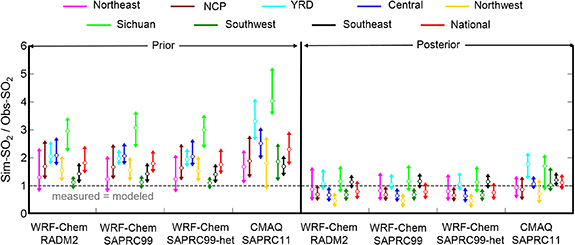
Specific to each region of China, the changes of model performance in the posterior were overall positive but inhomogeneous (figure 3). The most significant improvement occurred in the Sichuan basin, a place with the largest bias (NMB more than 200%) in the prior run. The posterior simulation dramatically reduced the surface SO2 concentration by ∼30 ppb in the Sichuan basin on an annual scale for all WRF-Chem and CMAQ simulations, and almost bridged the initial gap of 35 ppb. In all other regions, using the updated emission effectively reduces the surface SO2 by 2–21 ppb, and brings the predicted result much closer to the in situ observations, except Southwest China under the WRF-Chem scenarios.
Figure 3. Comparisons of simulated surface SO2 from prior forecast runs and posterior forecast runs to surface observations in different regions of China in 2009. The circle represent annual average of the ratio of simulated SO2 to observed SO2, and the line shows the range of its monthly averages. Different colors indicate different regions of China, including the Sichuan basin, NCP, Central China, YRD, Northwest China, Northeast China, Southwest China, and Southeast China.
Download figure:
Standard image High-resolution image
3.3. Evaluation with MODIS AOD
Beyond being a criteria gaseous pollutant, ambient SO2 could convert into particle phase via the formation of sulfate aerosol, which has adverse effects on air quality and human health. The top-down SO2 emission effectively corrected the simulated SO2 concentration, and thus would further have a corresponding impact on sulfate and columnar AOD. The simulated AOD from the prior and posterior simulations are further evaluated with the MODIS observations (figure S8). We added the dust AOD estimated by Ginoux et al (2012) to the calculated AOD in CMAQ to fill in the missing dust sources in the model. The MODIS observed AOD was higher in the NCP region, the Sichuan basin and Central China, due to high PM2.5 concentration and humidity. The simulated AOD from both prior and posterior runs had similar spatial patterns, consistent with the observation, but the magnitude of the posterior prediction (AOD = 0.38–0.39) was closer to the observation (AOD = 0.35). The Taylor diagram in figure 2(c) again shows the improvement of model performance in AOD. The updated SO2 emission positively reduced the NMB from 17%–20% to 14%–17%, and slightly decreased the normalized RMSE and STD from 0.72–0.91 to 0.69–0.88 and from 0.91–1.19 to 0.88–1.13, respectively. The correlation coefficients between the predicted and observed AOD were similar in both simulations, with the value of 0.64–0.74, which indicated good model performance at capturing the spatial variability.
4. Conclusions and discussions
We employed two regional chemical models WRF-Chem and CMAQ with a total of four different chemical mechanisms or four independent model experiments to evaluate the efficacy of top-down SO2 emission that was derived by using satellite (OMI) observation and GEOS-Chem (a global chemical model) adjoint model. For 2009, the satellite-constrained SO2 emission captures a 50% reduction occurred in China, compared to a bottom-up estimation from MEIC. We conducted four sets of simulations with different models and/or mechanisms, each of which contains two parallel simulations using the two SO2 emissions, and further applied multiple observations to evaluate the potential of the updated emission for air quality forecast and optical property analysis. The satellite-constrained SO2 emission overall improves the model performances significantly in vertical column SO2 and surface SO2, with the NMB decreased by 194%–214% and 96%–119%, and the normalized RMSE decreased by 1.54–1.83 and 1.17–1.32, respectively, as compared to that using the bottom-up emissions. The corrected ambient SO2 concentration further leads to the improvement in predicting PM2.5 and reduces the NMB of AOD simulation to 14%–17%.
In general, numerical simulation of SO2 contains many aspects in its complete process, starting from pollutant emission, undergoing transportation, diffusion and chemical transformation, and finally removed from the atmosphere through dry and wet depositions. The error and uncertainty in each aspect will affect the fate of forecasted SO2. Hence, even the SO2 emission has no errors, the simulated SO2 may still have uncertainties from non-emission sources. Therefore, we quantify 'whether the efficacy of satellite-based inversion of SO2 emission is dependent of models' by focusing on the analysis in two parts. The first part is the multi-model comparison, analyzing similarities and differences of simulated SO2 with prior emission using different models and different physical/chemical mechanisms, from which we can assess the influences of different parameterization schemes. To be specific, the similarity or difference identified here include the influences of (a) with and without interaction between meteorology and chemistry, (b) different lumped gaseous chemical mechanisms, (c) different aerosol chemical schemes and aerosol size distribution schemes, (d) with and without SO2 heterogeneous reaction forming sulfate aerosol, and (e) other potential differences caused by different model structures. The second part is the inter-comparison of simulated SO2 fields with the priori and the posterior emissions, and use independent observations to evaluate the improvement of the simulation results by using the top-down emissions. Through the above multi-model and inter-model comparisons, we pointed out that: (a) the magnitude and variation of simulated SO2 are similar (STD less than ±10%) and well correlated (r = 0.66–0.84) in different models (table S3) and the bias directions (overestimation) are consistent for all models, and (b) the posterior SO2 emissions show significant and consistent improvements in SO2 and AOD simulations in all these models. Thus, we conclude that the impacts of uncertain physical/chemical mechanisms in different models on simulated SO2 fields are much smaller than the impacts of uncertainties in emissions on a monthly mean scale, and the efficacy of satellite-based inversion of SO2 emission appears to be high for CTMs that use similar or identical emission inventories. In other words, there are common emission errors among different CTMs in the regions like Asia, and this study quantitively shows that the top-down emission analysis based on one CTM can be effective to correct these common errors (especially biases), and consequently can be valuable for updating the emissions in other CTMs that have different meteorology and chemistry.
It should be noted that our assessment of the emission efficacy is mainly to evaluate those modeled variables that mostly reflect the change of emissions (e.g. surface SO2 and columnar SO2 and AOD in this case). Emissions are not the single culprit for the model errors, especially those errors that are not strongly related to emissions. Indeed, for both WRF-Chem and CAMQ, the posterior emissions lead to the reduction of surface sulfate by 24%–31% throughout the year (figure S9) and the reduction of surface PM2.5 concentration by 1.1–2.5 μg m−3 (figure S10). These simulation differences are comparable to the difference due to the heterogeneous formation of sulfate that can contribute 6%–25% to the total sulfate in the posterior simulations. Therefore, the efficacy of the emission should NOT be interpreted as the robustness to improve every aspects of the model. To the contrary, the efficacy of the emission is only an integral part (and in many cases the first step) needed to assess and improve the physical and chemical processes in the model, thereby reducing overall systematic or persistent bias in the model.
Finally, to our knowledge, this study is the among the first to assess the extent to which the top-down estimate of emission or the satellite-constrained updates of bottom-up emission can be applied for regional air quality simulations. We show here that the efficacy of the top-down estimate of SO2 emissions from a global model such as GEOS-Chem appears to be robust for improving the regional air quality models that may have different chemistry and physics from the model used for the inversion. While more studies with more models and cases are needed to further evaluate the conclusion here, our results here suggest that in near future, as the routine retrievals of aerosols and short-lived species such as SO2 and NO2 will be soon available from geostationary platforms over Asia (e.g. GEMS, Kim et al 2020), Norther America (TEMPO, Zoogman et al 2016), and Europe (Sentinel-5, Ingmann et al 2012) at hourly resolution with unprecedented spatial resolution, it is foreseeable that an era of inverting emission from these retrievals or updating the bottom-up emissions with these measurements (such as through the framework of GOES-Chem adjoint model) is emerging to effectively reduce the temporal lags in the current bottom-up approach for emission estimate, thereby reducing the model persist errors from the model initial conditions of emissions. This would be especially important for the air quality modeling during the future events of natural hazards or public heath emergencies (that may be similar as the COVID-19 pandemic leading to large changes of anthropogenic emissions).
Acknowledgments
This work was supported by the National Key R&D Program of China (2019YFA0606804 and 2018YFC0213802), the National Natural Science Foundation of China (41975171 and 41705128), and the Major Research Plan of National Social Science Foundation (18ZDA052). J Wang and Y Wang's participation is made possible through the in-kind support at the University of Iowa.
Data availability statement
The data that support the findings of this study are openly available at the following URL/DOI: http://nuistairquality.com/sjxz.