Towards a semantic indoor trajectory model: application to museum visits

Abstract

In this paper we present a new conceptual model of trajectories, which accounts for semantic and indoor space information and supports the design and implementation of context-aware mobility data mining and statistical analytics methods. Motivated by a compelling museum case study, and by what we perceive as a lack in indoor trajectory research, we combine aspects of state-of-the-art semantic outdoor trajectory models, with a semantically-enabled hierarchical symbolic representation of the indoor space, which abides by OGC’s IndoorGML standard. We drive the discussion on modeling issues that have been overlooked so far and illustrate them with a real-world case study concerning the Louvre Museum, in an effort to provide a pragmatic view of what the proposed model represents and how. We also present experimental results based on Louvre’s visiting data showcasing how state-of-the-art mining algorithms can be applied on trajectory data represented according to the proposed model, and outline their advantages and limitations. Finally, we provide a formal outline of a new sequential pattern mining algorithm and how it can be used for extracting interesting trajectory patterns.

1 Introduction

It has long been of paramount importance for museums to know their visitors, meaning to study and understand their motivations, expectations, engagement, and satisfaction. In this regard, mobile devices offering location-based services (e.g. way-finding, contextualized content delivery) are becoming an invaluable tool for museums, since they provide them with access to an unprecedented wealth of visitors’ movement data. Similar opportunities have appeared in other domains of indoor human mobility such as shopping malls, sports and concert arenas, hospitals, airports, universities [30]. For big museums in particular, the collected visit datasets can be very large, due to the daily tracking of tens of thousands of visitors. Moreover, depending on the implemented system, contextual/semantic data and indoor environment-related data can be gathered in addition to the positional data. What is more, in many cases the localisation process may suffer from imprecision, as it is being altered by the museum’s architecture, especially when it has not been originally designed for housing art collections. This places the movement analysis problem in the field of Big Trajectory Data analytics.

So far, trajectory-based human mobility data analytics research has mainly focused on outdoor trajectories, driven by the fact that Geographic Information Science (GIS) has traditionally only supported outdoor spatial information. This type of research differs considerably in indoor environments, mainly due to interior architectural components constraining (or otherwise affecting) the way people move. For example, an indoor trajectory model has to consider multiple ways of entering a room, floor changes, specific locations of building entrances/exits, sensor coverage gaps due to obstacles, sensor detection area overlaps due to different floors, movement data of varying spatial granularity, and other challenges. In addition, indoor trajectory analytics may gain from avoiding cumbersome calculations over geometric representations of space and objects within it, that are typical of outdoor environments. Instead, operations such as intersection, containment, and proximity can be simplified in order to prioritize the non-geometric aspects of movement [28], instead of metric aspects typically focused on Euclidean distances from potential targets.

Moreover, in order to reason about movement in information-rich domains, a trajectory model must also account for multiple types of contextual and semantic information. As identified by Peuquet in [47] and further explored in [5, 6], there are three fundamental sets pertinent to movement, representing the where (set of locations), when (set of instants or intervals), and what (set of objects) of spatiotemporal data. This is true across applications as well as across application domains. Distinguishing between semantics of time, semantics of places, and semantics of moving objects (MOs), in addition to the semantics of movement itself, could empower a synergistic interplay between different types of semantics. Such semantic information can be derived either from the MO’s environment or from external data sources. It can then be used to add a meaningful dimension to raw Big Trajectory Data. Unfortunately, semantic trajectory models have - to a large extent - targeted outdoor settings.

This has resulted in an emphasis on the enrichment of GPS data, the identification of stops and moves, the identification of transportation means, and other conceptual modeling issues that are, either not interesting or not transferable, in indoor settings. For example, a MO does not traverse as long traveling distances, nor does it reach as high speeds, when indoors. Therefore, a museum visitor might still be visiting, whether standing in front of a particular painting or steadily walking across a hall full of paintings, and a shopping mall client might still be shopping, whether standing in front of a specific product stand or steadily walking across retail corridors. Thus, the distinction between walking and standing still is not nearly as useful as the distinction between stops and moves typically found in outdoor trajectories. On the other hand, the adoption of some modeling approaches, such as the segmentation of trajectories into episodes and the use of semantic annotations, seems to be promising for indoor environments as well.

Identifying proper trajectory modeling aspects for enabling advanced museum visitor mobility analytics depends a lot on the specific goals of the analysis. These goals mainly concern the improvement of the visitor experience, the managerial decision making, and the visitor crowd management processes. For all three types however, the indoor context and the semantic aspect of movement remain key modeling elements. By intertwining the model of visitor trajectories with a model of the museum space, an individual visitor may enjoy personalized location-based services such as a dynamic itinerary update based on the congestion levels in the exhibition spaces. At the same time, the museum management may optimize emergency evacuation routes, taking into account each visitor’s profile (e.g. reduced mobility). Such goals can only be achieved if the trajectory model is actually aware of the indoor network topology as well as aware of the contextual information regarding the space (e.g. congestion level, function), the visitor (e.g. demographics, guide usage), and the movement itself (e.g. resting, being lost).

In this paper, we present a new model for spatiotemporal indoor trajectories enriched with semantic annotations, called Semantic Indoor Trajectory Model (SITM). The proposed model makes use of a standardized indoor space modeling framework, instead of modeling space on a 2D coordinate reference system, as is typically the case. It integrates semantic annotations at different levels in order to allow a detailed description of the movements. Moreover, the model is developed with the Big Trajectory Data mining and analysis task support in mind. To achieve this, we first run existing pattern mining algorithms on trajectory data following a SITM-based formalism, and we identify their advantages and limits with respect to the expressiveness of SITM. Finally, we propose corresponding improvements to be integrated in new trajectory pattern mining algorithms.

The main contributions of the paper are:

• 1. A new model for spatiotemporal indoor trajectories enriched with semantic annotations, called SITM.

• 2. A validation of the proposed model by its instantiation on real data.

• 3. A study of how current mining algorithms can be applied on trajectory data expressed under SITM.

• 4. A formalization of the problem of mining the semantic indoor trajectories expressed under SITM.

The rest of this paper is divided as follows: Section 2 presents an overview of the related work and its limitations. Section 3 introduces SITM. Section 4 introduces the Louvre case study and the corresponding model instantiation. Section 5 explains how existing pattern mining algorithms can be applied on trajectories represented by SITM and provides insight for designing a new family of such algorithms. Finally, Section 6 concludes with the key issues addressed in this work.

2 Related work and background

In this section, we describe the state-of-the-art in modeling indoor spaces and (outdoor) semantic trajectories.

2.1 Indoor space models

In order to represent movement phenomena in terms of trajectories, first a formal spatial model is needed to provide an abstraction of their physical environment. Every trajectory model proposed in the literature, either explicitly or more usually implicitly, uses a certain model of location and therefore space. In this regard, a fundamental distinction exists between quantitative and qualitative spatial representation approaches. The former are preferable when precise spatial information is important, while the latter when it is unnecessary or unavailable [13].

A qualitative spatial representation formalism, coupled with qualitative relations between spatial objects and qualitative reasoning about spatial knowledge, constitutes what is known as Qualitative Spatial Reasoning (QSR) [53]. Two of the most widespread qualitative spatial calculi are RCC (Region Connection Calculus) [14] and n-intersection [20].

RCC theory, in particular, considers spatial regions as its primary spatial primitive and the reflexive and symmetric is connected to dyadic relation as its primitive relation [16]. Based on it, various constraint languages have been defined. For example, RCC-8 defines eight JEPD (Joint Exhaustive and Pairwise Disjoint) relations: is disconnected from, is externally connected with, partially overlaps, equals, is a tangential proper part of and its inverse, is a non-tangential proper part of and its inverse.

Alternatively, n-intersection theory is based on point-set topological theory and considers a spatial region as a 2D point set x embedded in $\mathcal {R}^{2}$, related to its interior, its boundary, and its exterior [21]. In particular, the 4-intersection formalism ignores the exterior, and based on the intersection combinations of the interiors and boundaries of two regions, results in eight binary topological relations: disjoint, touch (meet), overlap, contains, insideOf, covers, coveredBy, equal [22], equivalent to those of RCC-8.

From a more applied perspective, most indoor spatial data models can be classified into geometric ones and symbolic ones [1]. The former focus on representing the geometry of indoor features using primitives such as points, lines, areas, and volumes. The latter focus on representing the ontological aspects of spatial units and the topological relationships between them, maintaining a more abstract view of indoor space [2]. Symbolic indoor space models in particular, are typically either set-based or graph-based (when capturing topological information). Hybrid models represent both symbolic concepts and geometric properties. Geometric and symbolic indoor space models largely correspond to the aforementioned quantitative and qualitative approaches of representing space in general, but focus on the conceptual data structures that hold the spatial information rather than on its mathematical formalism.

Furthermore, a line of research works on indoor space modeling ([8, 11, 29, 36, 57], etc.) has culminated into the development of IndoorGML [37, 38], an OGC standard aimed at representing and allowing the exchange of geoinformation for indoor navigational systems. Its core module considers an indoor space as a set of non-overlapping cells that represent its smallest organizational/structural units: S = {c₁,c₂,...,c_n}, c_i ∩ c_j = ∅. Technically, IndoorGML describes a hybrid indoor space model since it captures the topological information of cells as well as an optional quantitative description of their spatial characteristics. The cell space and the topological relationships among its objects are represented by one or more Node-Relation Graphs (NRGs), simplifying complex spatial relationships based on graph theory concepts [36] and the Poincaré duality in particular. More specifically, a cell (e.g. room) becomes a node and a cell boundary (e.g. a thin wall) becomes an edge. If cell boundary semantics are also taken into account (e.g. doors, walls, ramps) then a connectivity and/or an accessibility NRG may be derived as well. Connectivity suggests that there exists an opening in the common boundary of two cells. Accessibility additionally suggests that the opening can be crossed by the MO.

Moreover, IndoorGML’s Multi-Layered Space Model (MLSM) is the description of multiple interpretations of the same physical indoor space, through the instantiation of multiple cell decompositions and corresponding NRGs. Each NRG is treated as a separate graph layer. Nodes belonging to different layers are connected via inter-layer joint edges. While intra-layer edges represent either adjacency, connectivity, or accessibility relations between non-overlapping cells, joint edges denote potential locations where a physical object might actually reside. Therefore, given that a physical object may be in only one cell of each layer at any given point in time (called the active state), joint edges express all the valid active state combinations (called overall states) and are derived by pairwise cell intersection. Equivalently, a joint edge represents any of the eight binary topological relationships derived by the n-intersection model [20], except for disjoint and meet, because a physical object can not simultaneously coexist in two cells that are completely disjoint or simply touch each other. In Fig. 1 for example, if a visitor is inside the hall represented as node 5 in layer i+ 1, then the joint edges suggest that he can only be in either 5a, or 5b, or 5c in layer i.

Fig. 1

Structured (left) or ad-hoc (right) representation of a hierarchical space

As illustrated in Fig. 1, the MLSM can be used to represent spatial hierarchies. In [31], the authors define an IndoorGML hierarchical graph as a direct adaptation of the hierarchical graph definition of [58]. The overlap relation is excluded from the joint edges of a hierarchical graph, which are explicitly mentioned to represent equal, coveredBy and inside relations. For instance, in Fig. 1, nodes 1, 2, and 3 in layer i+ 1 would be assumed to connect via three joint equal edges to their counterparts in layer i, while nodes 4 and 5 would be assumed to connect to nodes 4a, 4b and 5a, 5b, 5c respectively, via joint coveredBy edges. However, the authors only provide some general partitioning criteria for how to properly choose which hierarchical levels to include in the model, such as splitting cells that have multiple properties or that are too big. On the same matter, in [18] the authors recognize that spatial cell subdivision may be driven both by the architectural structure of the building and by the function of space. They propose a categorization of specific criteria to automate this procedure: geometry-driven criteria (e.g. split if some cell dimension surpasses a certain value), topology-driven criteria (e.g. split depending on which cells a cell is connected to before/after the split), semantics-driven criteria (e.g. split depending on what type of cells a cell is connected to) and navigation-driven criteria (e.g. split if a cell has both walkable and non-walkable parts). Despite the fact that they focus on furnished 3D indoor spaces, their categorization can also be useful for 2D representations of space, but the specific splitting mechanism may differ considerably from case to case.

2.2 Semantic trajectory models

In the last decade, accounting for the semantics of movement has received a lot of attention in the trajectory data modeling and analytics literature. Pivotal to this, has been viewing a trajectory as “the user-defined record of spatiotemporal evolvement of the position of a MO, during a given time interval of its lifespan, and in order to achieve a certain goal” [55]: $[t_{begin}, t_{end}] \rightarrow space$. In the same work, a purposefully generic way of semantically segmenting a trajectory into stops and moves was also established, leaving its implementation to be specified at the application level. For example, Alvares et al adopted in [3] the previous model and defined stops based on temporal stay value thresholds. Similarly, Bogorny et al adopted in [9] the conceptual trajectory model from [55] and associated stops with important visited places, before extending it with fundamental data mining concepts (in the form of classes, attributes, methods) in order to support the tasks of frequent patterns, sequential patterns, and association rules. Thus, it defined a semantic trajectory as a sequence < I₁,I₂,...,I_n> where each I_k represents a stop or a move having a spatial and a temporal dimension.

More recently, in [5, 6], Adrienko et al propose a general conceptual modeling framework aimed at connecting the analysis of movement data with its spatiotemporal context, which is defined as the physical space and time where movement takes place, together with the objects and events that co-exist in it. Their framework exhaustively categorizes the types of information that can be represented by movement data. First, it breaks movement down to its most essential elements: the set of locations S (space), the set of time units T (time instants or intervals), and the set of objects O (physical and abstract entities). The elements of these sets may have properties represented as spatial, temporal, or thematic attribute values, which in turn may involve other elements of S, T, O. Within this framework, movement in general can be seen as a collection of spatial events, represented by the mapping $\tau : T \rightarrow S$ (single mover) or $\mu : O \times T \rightarrow S$ (multiple movers). Semantic modeling is however not addressed, apart from dynamic thematic attributes which represent any attribute available in the movement data or “any other existing or conceivable thing”. These can be thought of as the equivalent of semantic annotations in other semantic trajectory models.

In [62, 64], the authors propose a modeling and computing platform for inferring semantic concepts (similar to the ones introduced in [55, 61]) from raw GPS data. The platform includes a hybrid trajectory model comprised of three (sub)models. The raw data model encapsulates a low-level representation of trajectories derived from the characteristics of raw mobility data, based on temporal (e.g. hourly/daily/monthly) or spatial (e.g. geofenced) trajectory division points. The conceptual model encapsulates a mid-level semantic abstraction of trajectories as series of episodes. The semantic model encapsulates the spatiosemantic behavior of trajectories via semantic annotations of them or of their episodes.

SeMiTri [63] is an application-independent framework for the semantic enrichment of raw GPS trajectories in the form of annotations based on spatial and temporal properties of raw data streams. The enrichment happens either at a low level via the notion of a semantic place

$$ sp_{i} \in P = P_{region} \cup P_{line} \cup P_{point} $$

which represents a meaningful geographic object (with a Region Of Interest (ROI), a Line Of Interest (LOI), or a Point Of Interest (POI) as its extent), or at a high level via the notion of an episode, which abstracts a subsequence of the spatiotemporal trajectory’s points that are highly correlated with respect to some identifiable spatiotemporal feature (e.g. velocity, time interval).

The conceptual semantic trajectory model proposed by Spaccapietra and Parent in [54] and refined in [45] is similarly structured as a sequence of potentially annotated timestamped coordinate positions or episodes. An annotation is defined as any additional data (captured or inferred) that enrich the knowledge about a trajectory or any part thereof. It can be an attribute value, a link to an object, or a complex value composed of both. More specifically, the trajectory model mainly consists of the following tuple: (trajectoryID, movingObjectID, trajectoryAnnotations, trace: LISTOF position (instant, point, δ, positionAnnotations), semanticGaps: LISTOF gap (t₁, t₂), segmentations: SETOF segmentation (segmentationID, episodes: LISTOF episode (t₃, t₄, definingAnnotation, episodeAnnotations))) where an episode is defined in [63] as “a maximal subsequence of a semantic trajectory, such that all its spatiotemporal positions comply with a given predicate, bearing on the spatiotemporal characteristics of the positions”. Also, positionAnnotations, episodeAnnotations, and trajectoryAnnotations are the sets of annotations associated to the three corresponding granularity levels of semantic enrichment. Lastly, temporal gaps in the movement track greater than the sampling rate of raw data, are said to be either accidental (holes) or intentional (semantic gaps), in which case their list makes part of the main trajectory model.

CONSTAnT [10] is a conceptual semantic trajectory model that resembles the model in [45], but supports more strictly defined types of trajectory semantics. A trajectory T is defined as an ordered list of timestamped (x,y) coordinate points. Enriched with contextual information, a semantic trajectory is defined as the tuple ST = (tid,oid,S,g,d) where:

• tid is the trajectory’s identifier

• oid is the moving object’s identifier

• S is the non-empty list of semantic subtrajectories

• g is the required general goal of the trajectory (i.e. the reason/objective of the movement)

• d is the device that generated the trajectory

Moreover, a semantic subtrajectory s ⊂ ST is defined as a list of consecutive semantic points, that corresponds to at least a goal, or a means of transportation, or a behavior, if not to multiple ones. Lastly, a semantic point p ∈ s is defined as a coordinate point, annotated with a set of so-called environments related to where it was collected and/or with a set of places where it is located.

More recently, MASTER [43] is a conceptual semantic trajectory model which has been converted to a logical RDF Schema and implemented using a middleware that stores RDF data into multiple NoSQL databases. It focuses on the heterogeneity of the semantic information of trajectories with particular attention being paid in the relationships between moving objects. More specifically, it introduces the notion of aspects to represent real-world facts relevant to the trajectory data analysis, and the notion of aspect types to characterize them with a description and properties, akin to a semantic taxonomy. This gives rise to the notion of semantic meanings, the associations between aspects and their types i.e. context. In MASTER, a multiple aspect trajectory is defined as a tuple mat = (P,S_LTA,mo,desc) where:

• P =< p₁,p₂,...,p_n> is a sequence of timestamped (x,y) coordinate points

• S_LTA = {SM_lta} is a set of long term (i.e. not changing) aspects

• mo is the moving object

• desc is an aspect description

Apart from the geometric nature of the trajectory data, MASTER is actually compatible with the model we propose in this work, because it focuses on the modeling of the relations between moving objects and a handful of other concepts such as events, that we leave largely unspecified, whereas it does not consider data at multiple granularity levels and therefore could be implemented at the lowest granularity level in parallel to our model.

Finally, [60] provides the outline of a moving objects database system, aimed at integrating multiple movement data models (e.g. road network models, region-based outdoor models, indoor models) paying attention to the support of semantics and multiple descriptive attributes. A data type called mpoint is defined for representing spatiotemporal trajectories having m attributes A₁,...,A_m. The system is intended to also include a pre-processing tool for the detection and reparation of GPS data error, a supervised-learning classifier for handling natural language queries, and a prediction model for indicating the 3D R-tree’s leaf where nodes are stored. This goes to show that semantic trajectories are gradually starting to be supported at the lowest system levels.

More generally, in the earlier semantic trajectory modeling literature, semantics were largely exhausted in the names and types of the geographic places of interest related to the MO’s physical stops. Whereas other types of contextual information, or topological and geographical relations between places, were rarely taken into account. Efforts have since been undertaken to integrate movement ontologies, linked open data, information extracted from social network platforms, or complementary case-specific datasets, with spatiotemporal trajectory data. Even the basic concept of episodes can be viewed as a generalization from stop-move segments to more diverse and heterogeneous semantics. In addition, such semantics have largely concerned outdoor contexts, as made evident by the terminology (e.g. traveling objects [55]) and definitions introduced. On the contrary, a model for semantic trajectories in indoor environments needs to at least consider the building’s topology and space semantics. The interior of buildings is typically divided into clearly delimited spatial entities such as rooms, halls, corridors, floors. This physical segmentation already holds a considerable amount of semantic information. Naturally, more types of semantics can be expected to become relevant given the increasing interest in context-aware location based services and applications (e.g. context-aware museum guidance [34]). As a result, Big Trajectory Data are characterized by their variety and not just volume.

With this in mind, it is safe to argue that in the near future, many applications will benefit from a trajectory model oriented both towards indoor environments and towards the semantic aspects of movement. [15] is one of the very few such works, proposing a geographic ontology-based conceptual trajectory model called STriDE, which focuses on the representation of moving objects and dynamically changing environments. STriDE actually extends the Continuum model [27], which represents dynamic entities using ephemeral timeslices composed of an object identity, a set of object properties, a geometric spatial representation, and the timeslice’s valid period. Filiation relationships between consecutive timeslices associated with the same entity, are used to represent the entity’s spatial or semantic evolution. In STriDE, a semantic trajectory is defined as a set of timeslices having a starting and an ending spatiotemporal point.

Furthermore, for most semantic trajectory models, the sole spatial primitive is a 2D coordinate position relative to the GPS’s or to the specific application’s coordinate reference system. But, raw indoor movement tracks are often collected in symbolic form, either due to indoor positioning technologies being better suited for compartmentalized tracking (e.g. proximity sensor readings), or due to data compression needs. The latter is particularly important in the context of Big Trajectory Data, because the indoor topology can be used to reduce the massive storage needs, in a way much similar to a road network [52]. At the same time, knowing in advance the spatial entities that the MO could find itself in (e.g. a list of rooms) makes encoding them as symbols conceptually and computationally more practical. Therefore, symbolic and hybrid indoor space models become more attractive than geometric ones for modeling movement in indoor environments.

3 Semantic indoor trajectory model

In this section, we define a new model for semantic trajectories in indoor environments, named Semantic Indoor Trajectory Model (SITM), aimed at supporting:

• all types of indoor settings;

• both human and inanimate MOs;

• mining and analysis applications using statistical and reasoning approaches in order to provide insight both at the individual and collective level.

More particularly, SITM needs to support spatiotemporal types of analysis and semantics-based types of analysis, at multiple levels of spatiosemantic granularity, for multiple MOs, and at the same time account for trajectory data quality and uncertainty issues. Therefore, it consists of a semantically enriched representation of indoor space, and a semantically enriched sequence representing an individual MO’s spatiotemporal presence.

The semantically enriched representation of indoor space that we propose is a layered multigraph. Its nodes symbolically represent indoor spatial regions, and its edges represent topological relationship information between those regions. Static semantic information about the regions is represented through node classes and attributes as well as node-edge grouping into layers. The proposed representation is compatible with OGC’s IndoorGML standard and can be viewed as an extension of it. It is described in Section 3.1.

The semantically enriched representation of an individual MO’s trajectory that we propose is a couple consisting of a trace of consecutive presence intervals inside the indoor regions represented by the graph’s nodes, and a set of semantic annotations describing the trajectory in its entirety. It uses the aforementioned indoor space representation and is described in Section 3.2.

3.1 Indoor space modeling

Based on the modeling framework provided by the IndoorGML standard and in particular its Multi-Layered Space Model (MLSM), we represent a 2D multiple floor (i.e. 2.5D) indoor space as follows:

Definition 1 (2D multiple floor indoor space)

A 2D multiple floor indoor space is represented as a layered multigraph G = (V,E) where

$$ V = \bigcup\limits_{i=0}^{m} V_{i} $$

(1)

and

$$ E = E^{top} \cup \bigcup\limits_{i=0}^{m} E^{acc}_{i} $$

(2)

Each $G_{i}=(V_{i}, E_{i}^{acc})$, 0 ≤ i ≤ m, constitutes an accessibility Node-Relation Graph (NRG), and E^top represents binary topological relationships between two cells of different layers.

The graph G is composed of m + 1 different layers of nodes and edges, each represented by a NRG G_i and corresponding to a different decomposition of the indoor space. On the one hand, node v ∈ V_i represents a cell belonging to the i-th layer and an edge $e \in E^{acc}_{i} \subseteq V_{i} \times V_{i}$ represents the accessibility between two cells of the i-th layer. On the other hand, a joint edge $e' \in E^{top} \subseteq V_{i} \times V_{j}$ represents a binary topological relationship between two cells of different layers (i≠j). Figure 2 illustrates an example of such an indoor space graph representation consisting of five hierarchical layers: Region of Interest, Room, Floor, Building, Building Complex, detailed in Section 4 but in general G does not need to be hierarchical.

Fig. 2

A 2D multiple floor hierarchical indoor space representation

In the proposed indoor space model, we adopt IndoorGML’s implicit assumption that each node belongs to a single layer ($\bigcap \limits _{i=0}^{m} V_{i} = \emptyset$). If a node is relevant to multiple layers, then it is essentially replicated in each one and all the copies are connected to each other via equal joint edges. Moreover, given that cells represent the physical reality of planar space (instead of a conceptual space) and that same-layer cells do not overlap at all, an intra-layer edge $e \in E^{acc}_{i}$ actually presupposes the meet relation between its two cells, because they need to share a common surface for the MO to be able to physically transition between them.

At the same time, as explained in Section 2, in IndoorGML, a joint edge $e^{\prime } \in E^{top}$ signifies that either one of the overlap, contains, insideOf, covers, coveredBy, or equal topological relations holds between the two cells that it connects. Thus, intra-layer edges and inter-layer edges are always of a different type, and therefore G can be considered as an edge-coloured multigraph which can be mapped to a multilayer network [32].

For the indoor space representation, an important modeling decision is whether G is directed or not. Although IndoorGML does not explicitly assume either case, it considers undirected edges in all of its examples. As far as intra-layer edges go, we can think of adjacency and connectivity as being symmetric relations. However, accessibility is not symmetric since often indoor movement is only unidirectionally possible due to technical, safety or other limitations. In Fig. 1 for example, Room4 (Salle des États) houses the Mona Lisa and accommodates a vast number of visitors on a daily basis. To facilitate their flow, entering it from Room2 is often prohibited by the museum personnel while exiting it that way is allowed. Therefore, we assume directed accessibility NRGs. As far as joint edges go, while overlap and equal can be thought of as symmetric binary relations, contains and covers can not. Therefore, we also assume directed joint edges (as can be seen in Fig. 2). If we wanted to simply model intersection non-emptiness, instead of the specific nature of the relation, then undirected joint edges would suffice.

In our model, we define a layer hierarchy as k + 1 ordered layers G_i (0 ≤ i ≤ k, k ≥ 2) of G that are only consecutively connected by joint edges. Similar to [31], we exclude overlap relations from layer hierarchies, but contrary to it, we also exclude equal relations to prohibit node repetition and instead favor a proper hierarchy. Instead of [31]’s inside and coveredBy, we assume contains, covers, and a corresponding top to bottom joint edge direction.

Furthermore, we account for the fact that virtually any indoor environment is characterized by a basic three-layer hierarchy consisting of: a Building layer, a Floor layer, and a Room layer. The latter is loosely named as it may actually contain any type of room-level navigable spatial cell, such as rooms, chambers, halls, lobbies, cellars, terraces, corridors, hallways, big staircases. Therefore, G includes 3 layers representing static hierarchical levels of spatiosemantic granularity. Other layers are optional and may also integrate with this core layer hierarchy, in which case k > 2.

It is thus evident that there can be layer hierarchies that comprise either topographic layers, or semantic layers, or both. Our core hierarchy is basically a topographic one. The Building and Floor layers are spatially defined, since the architectural structure alone is mostly enough to determine which space constitutes a building and which space constitutes a floor. The Room layer is also predicated spatially, but in a looser way since it may on occasion contain cells whose boundaries are not necessarily physical (e.g. functionally independent subspaces of a big hall or of a great room).

Additionally, two optional layers are proposed for typical cases, as presented in Fig. 2: a Building Complex root layer and a Region of Interest (RoI) leaf layer. We define the Building Complex layer to represent the indoor space of a site comprised of multiple buildings, such as a hospital spanning multiple attached wings or a university campus spanning multiple independent edifices. We define the RoI layer to represent navigable sub-room level spatial cells of application-specific interest, such as “you-are-here” map installations in a shopping mall or individual exhibit displays in a museum (as detailed in Section 4.2 and Fig. 7). The Building Complex and RoI layers are only relevant per case, and can be properly integrated into the core layer hierarchy: Building Complex→ Building→ Floor→ Room→ RoI. In that case, a Floor object in Fig. 2 describes a single building’s floor level (e.g. FloorA1≠FloorB1).

A static predefined layer hierarchy, like the one presented in Fig. 2, as opposed to local ad-hoc node subdivisioning, allows a structured reasoning about the trajectories at multiple levels of granularity. By only allowing proper part types of relationships, we allow inference of a MO’s location at all levels of granularity above the detection data level. This in turn allows developing reasoning mechanisms to cope with missing or uncertain location information. It also enables the identification of certain types of movement patterns at the Room level for instance, and at the same time of other types of patterns at the Floor level, all from the same trajectory dataset. Furthermore, a standard layer hierarchy makes the model generalizable to different tracking technologies and infrastructures, thus enabling the fusion of heterogeneous Big Trajectory Data.

In addition, a static predefined layer hierarchy approach simplifies the indoor space model in case more than one hierarchical interpretations are needed. In specific, multiple layer hierarchies may be defined in parallel to each other via parallel joint edges that can additionally represent the equal and overlap relations. In that case, thanks to the transitivity of parthood (isomorphic to set inclusion) in classical mereology, each layer hierarchy only needs to connect to other layers or layer hierarchies at the lowest possible level, since an equal or overlap relation between two nodes means that an overlap relation also holds between any two of their respective predecessors. Related to this, our graph representation assumes that the indoor area designated by each node is fully covered by the areas represented by its child nodes, discussed in more detail in Section 4.2.

Finally, our SITM follows an entrance/exit node convention: only entrances may generate MOs and only exits may consume MOs. All other nodes are assumed to have equal input and output flows at the end of each day, which can serve for correcting tracking errors in the data. IndoorGML uses the concept of anchor nodes, to bidirectionally connect indoor and outdoor, and to contain information for transforming between the respective coordinate reference systems. Entrance and exit nodes can be viewed as specializations of anchor nodes and are meaningful even when the outdoor environment is not considered.

3.2 Semantic indoor trajectory modeling

Automatically collected raw movement data typically consist of spatiotemporal records, out of which individual trajectories can be extracted. Depending on the application and on the type of MO, only the evolution of its representative location may be relevant (e.g. museum visit analysis) or perhaps also its shape and parts’ movements (e.g. sports performance analysis). In the former case, a trajectory is typically represented as a sequence of timestamped spatial points. Due to a building’s clearly separated spaces however, we consider regions (instead of points) as our primary primitive spatial entities, in the spirit of Qualitative Spatial Representation [14] and IndoorGML’s cellular space [38], and according to the indoor space model proposed in Section 3.1.

In the following, we present the proposed model of semantic trajectories taking place in an indoor environment. We start by providing the formal definition of a semantic trajectory.

Definition 2 (semantic trajectory)

A semantic trajectory is defined as the couple of its spatiotemporal trace and the set A_traj of semantic annotations:

$$T_{ID_{mo},t_{start},t_{end}} = (trace_{ID_{mo},t_{start},t_{end}}, A_{traj})$$

where ID_mo is the identifier of the moving object, t_start and t_end are the trajectory’s starting and ending timestamps, $trace_{ID_{mo},t_{start},t_{end}}$ is a semantic trajectory trace representing the spatiotemporal aspect of the trajectory as a sequence of timestamped semantically annotated presence periods/intervals, and A_traj is a set of semantic annotations describing the trajectory in its entirety.

Assuming that no moving object can be in two different places at the same time, we use its identifier along with two limit-case timestamps, to identify each of its trajectories $T_{ID_{mo},t_{start},t_{end}}$, whose first element $trace_{ID_{mo},t_{start},t_{end}}$ will be more thoroughly described in the following definition.

The trajectory’s second element A_traj is a non-empty set of semantic annotations a_traj ∈ A_traj characterizing the trajectory in its entirety. Trajectory annotations are not confined within specific types of information, but would typically be chosen to represent an activity, a behavior, or a goal showcased by the complete trajectory. These terms are often ambiguously used in trajectory literature. In our model, we consider the following main types of semantic annotations:

• an activity concerning more targeted/conscious actions; for example:

  a_traj = “visit_temporary_exhibition”

• a behavior concerning less intentional actions or reactions; for example:

  a_traj = “follow_^′Masterpieces^′_guided_tour”

• a goal concerning motivations which affect the actions; for example:

  a_traj = “visit_Mona_Lisa”

The first two types describe the actuality of movement, whereas the third one instead describes the potentiality of movement. For example, many trajectories in the Louvre Museum are greatly affected by the visitor’s intention to see the Mona Lisa, irrespective of whether this goal will eventually be accomplished or disrupted due to overcrowding. Naturally, an entire trajectory may well be characterized by multiple types of semantics, as for example:

$$ \begin{array}{@{}rcl@{}} A_{traj} &=& \{behaviors:[``follow\_'Masterpieces'\_guided\_tour"],\\ &&goals:[``visit\_Mona\_Lisa"] \} \end{array} $$

Definition 3 (semantic trajectory trace)

Let us consider a 2D multiple floor indoor space represented as a layered multigraph G = (V,E) where

$V = \bigcup \limits _{i=0}^{m} V_{i}$ and $E = E^{top} \cup \bigcup \limits _{i=0}^{m} E^{acc}_{i}$.

A semantic trajectory trace is defined as:

$$trace_{ID_{mo},t_{start},t_{end}} = (e_{k},v_{k},t^{start}_{k},t^{end}_{k},A_{k})_{k \in [1,n]}$$

where v_k is the state where the MO ID_mo finds itself from $t^{start}_{k}$ until $t^{end}_{k}$, $e_{k} = (v_{k-1},v_{k}) \in \bigcup \limits _{i=0}^{m} E^{acc}_{i}$ is the transition i.e. boundary crossed that led the MO from state v_k− 1 to state v_k (e.g. which door, staircase, or elevator was used), and A_k is a potentially empty set of semantic annotations describing that specific stay.

As an example of a semantic trajectory and its corresponding semantic trajectory trace, let us consider a visitor’s 2-hour morning visit to the Louvre:

T_{vis0042,11:30:00,13:30:00} = (trace_{vis0042,11:30:00,13:30:00},

{goals : [“visit_temporary_exhibition”]})

trace_{vis0042,11:30:00,13:30:00} = {

(entrance01, “PH”, 11:30:00, 11:32:30, ∅),

(ticketcontrol02, “TE”, 11:32:30, 13:00:00, {mo : [“home_ticket”]}),

(ticketcontrol02, “PH”, 13:00:00, 13:02:00, ∅),

(opening02, “MS”, 13:04:00, 13:28:30, {activity : [“shopping”]}),

(opening01, “IPH”, 13:28:30, 13:30:00, ∅)}

The above semantic trajectory represents the movement of visitor vis0042 in the Louvre in order to visit the temporary exhibition. The visitor moves through 4 different zones, first appearing in and passing twice from the Pyramid Hall, then going to the Temporary Exhibition zone where he/she stays for a long time, and then going back again in the Pyramid Hall, before entering the Museum Shop area and exiting from the Inverse Pyramid Hall.

Not surprisingly, while in the Museum Shop the visitor did some shopping. It is not the trajectory model’s goal to show how to obtain such semantic aspects from the spatiotemporal context (they may even be simply provided), but rather to represent them in a way that enables and facilitates both their extraction and usage for analysis purposes.

To accommodate for trajectory holes and semantic gaps [54] as well as detection data uncertainty issues in general, the spatiotemporal trace is allowed to contain temporal gaps where the presence of the MO is unknown. This is the case in the above example when the visitor disappeared for a couple of minutes before entering the Museum Shop. Allowing for such gaps enables the design of analysis mechanisms [67] treating the uncertainty that is prevalent in Big Trajectory Data, especially those in raw form.

Next, we define a semantic subtrajectory as being for all practical purposes a semantic trajectory - similar to how a mathematical subsequence is itself a sequence - but necessarily referable to some other main semantic trajectory.

Definition 4 (semantic subtrajectory)

Given a semantic trajectory

$$T_{ID_{mo},t_{start},t_{end}} = (trace_{ID_{mo},t_{start},t_{end}}, A_{traj})$$

a semantic subtrajectory of it is defined as:

$$T'_{ID_{mo},t'_{start},t'_{end}} = (trace'_{ID_{mo},t'_{start},t'_{end}}, A'_{traj})$$

iff $trace^{\prime }$ is a proper subsequence of trace:

$t_{start} \leq t^{\prime }_{start} < t^{\prime }_{end} < t_{end}$ or $t_{start} < t^{\prime }_{start} < t^{\prime }_{end} \leq t_{end}$.

A subtrajectory’s set of semantic annotations $A^{\prime }_{traj}$ may or may not be the same as that of its main trajectory A_traj, contrary for example to [10] where they are enriched with different types of semantic information. Moreover, let us consider the previous example, as well as another visitor’s semantic trajectory:

T_{vis0043,13:00:00,13:33:00} = (trace_{vis0043,13:00:00,13:33:00},

{goals : [“visit_temporary_exhibition”]})

trace_{vis0043,13:00:00,13:33:00} = {

(entrance01, “PH”, 13:00:00, 13:02:00, ∅),

(opening02, “MS”, 13:04:00, 13:28:30, {activity : [“shopping”]}),

(opening01, “IPH”, 13:28:30, 13:33:00, ∅)}

This represents a more casual type of Louvre visitor who is simply shopping in its stores where a ticket is not required. According to a strict interpretation of Definition 4, the semantic trajectory of visitor vis0043 is not a subtrajectory of the semantic trajectory of visitor vis0042, because even though they share the same 3-zone pattern of visit $``PH" \rightarrow ``MS" \rightarrow ``IPH"$, vis0043 arrives at “PH” via a different edge and stays in “IPH” a little longer than vis0042.

Therefore in practice, depending on the application case, we need to mathematically relax the proper subsequence requirement according to a realistic interpretation of trace similarity. For instance, if we ignore the traversed edges and allow a temporal deviation of 5 minutes in the timestamps of each presence interval, then T_{vis0043,13:00:00,13:33:00} is indeed a semantic subtrajectory of T_{vis0042,11:30:00,13:30:00}, because their last timestamps differ only by 3 minutes.

Below we define an episode of a semantic trajectory as any particularly meaningful part of it.

Definition 5 (episode)

Given a semantic trajectory

$$T_{ID_{mo},t_{start},t_{end}} = (trace_{ID_{mo},t_{start},t_{end}}, A_{traj})$$

an episode of it is defined as:

$$T^{\prime}_{ID_{mo},t^{\prime}_{start},t^{\prime}_{end}} = (trace^{\prime}_{ID_{mo},t^{\prime}_{start},t^{\prime}_{end}}, A^{\prime}_{traj})$$

iff

• (1) $T^{\prime }_{ID_{mo},t^{\prime }_{start},t^{\prime }_{end}}$ is a semantic subtrajectory of $T_{ID_{mo},t_{start},t_{end}}$

• (2) $A^{\prime }_{traj} \neq A_{traj}$

• (3) $T^{\prime }_{ID_{mo},t^{\prime }_{start},t^{\prime }_{end}}$ satisfies a domain-dependent and user-defined spatiotemporal and/or semantic predicate $P_{ep}: T^{\prime }_{ID_{mo},t^{\prime }_{start},t^{\prime }_{end}} \rightarrow \{true, false\}$

Moreover, an episodic segmentation of a semantic trajectory is simply any subset of its episodes that covers it time-wise. Contrary to typical literature practice, we allow an episodic segmentation to contain episodes that overlap in time, since the exact same movement part may have multiple meanings depending on the broader context or on the scale at which it is examined.

If we consider the previous semantic trajectory example, the following is a non-overlapping activity-based episodic segmentation of it:

episode_seg = {

episode₁ (arrival):

T_{vis0042,11:30:00,11:32:30} = (trace_{vis0042,11:30:00,11:32:30}, {activities : [“arrive_Louvre”]})

trace_{vis0042,11:30:00,11:32:30} = {(entrance01, “PH”, 11:30:00, 11:32:30,∅)}

episode₂ (temporary exhibition visit):

T_{vis0042,11:32:30,13:00:00} = (trace_{vis0042,11:32:30,13:00:00}, {activities : [“visit_temporary_exhibition”], goals : [“visit_Salvator_Mundi”]})

trace_{vis0042,11:32:30,13:00:00} = {

(ticketcontrol02, “TE”, 11:32:30, 13:00:00, {mo:[“home_ticket”]}) }

episode₃ (departure):

T_{vis0042,13:00:00,13:30:00} = (trace_{vis0042,13:00:00,13:30:00}, {activities : [“shopping”,“exit_Louvre”]})

trace_{vis0042,13:00:00,13:30:00} = {

(ticketcontrol02, “PH”, 13:00:00, 13:02:00, ∅),

(opening02, “MS”, 13:04:00, 13:28:30, {activity :[“shopping”]}),

(opening01, “IPH”, 13:28:30, 13:30:00, ∅)}

}

Finally, even though it describes temporally continuous movement phenomena, SITM is still an event-based model: only a change of the spatial cell that the MO is located in, or a change of the semantic information regarding the MO’s presence in that cell, requires a new tuple. Hence, each tuple’s begin and end timestamps denote the natural time interval that corresponds to the MO’s physical presence given stable semantics. Such a representation suits most raw indoor mobility datasets, typically consisting of individual sensor detections.

4 The louvre case study

In this section, we present a compelling trajectory dataset from the world’s most frequented museum, the Louvre Museum.

4.1 Visitor movement dataset

In July 2016, the Louvre launched its official My Visit to the Louvre smartphone application, which takes advantage of a large Bluetooth Low Energy (BLE) beacon infrastructure¹ and the smartphone’s accelerometer and compass, in order to estimate the visitor’s precise position - in our case a (lat, long) coordinate pair - within the museum. This is accomplished via BLE Received Signal Strength Indicator (RSSI)-based trilateration, extended Kalman and particle filtering techniques. The app visualizes the position over a locally stored version of the museum map for navigation purposes. The Louvre has already been the object of visitor mobility research in the past leading to interesting conclusions [65, 66], but the current beacon infrastructure offers improved tracking coverage and continuity.

In the obtained dataset, raw geometric positions have already been spatially aggregated into 52 non-overlapping zones. Each zone corresponds to a large polygonal area of the museum, as detailed later in Fig. 4, specified by the museum administration in such a way so as to reflect a single exhibition theme (e.g. Italian paintings) but also only extend within a single floor.

Big museums can be a vast source of Big Trajectory Data, especially in terms of their volume and variety. The conceptual trajectory model presented in Section 3 aims at supporting the development of analysis techniques making use of such large datasets, produced on a daily basis by thousands of visitors. However, the results presented in this work are based on a dataset consisting of 4,945 visits, continuously collected from 19-01-2017 to 29-05-2017, each consisting of a sequence of timestamped zone detections i.e. detections of the visitor’s smartphone inside a certain zone. The duration of a visit ranges from 0 sec (considered as an error) to 7 hours 41 min and 37 sec, whereas the duration of a zone detection ranges from 0 sec (considered as an error) to 5 hours 39 min and 20 sec. The visits were performed by 3228 different visitors using both the iPhone and Android versions of the application. Out of those, 1,227 were returning visitors who made 1,717 second/third visits, although not necessarily on different days. The dataset includes 20,245 zone detections and 15,300 (intra-visit) zone transitions in total.

Unfortunately, only 30 out of the 52 zones appear in the movement dataset, with the -1 floor completely missing. Additional factors leading to a sparse movement dataset (both at the individual and collective level) may include the following: a visitor may launch and/or close the application mid-visit (due to battery depletion, sporadic navigation-only usage, etc.) resulting in its partial recording², 10.55% of the zone detections have a zero valued duration forcing us to filter them out as detection errors, the period of data collection³ results in lower adoption rates and potentially transitory phenomena. The sparsity of the data is partly illustrated in the power law distribution of the length of visit presented in Fig. 3, where it can be seen that 53.55% of the visits actually degenerate into a single zone detection. Out of that percentage, only 2.61% is due to erroneous detections of zero duration, therefore practically one out of every two visits has a length of only 1.

Fig. 3

Bar chart illustrating the dataset’s distribution of visit length

4.2 SITM model instantiation

Indoor space representation

In order to instantiate the SITM presented in Section 3.2 for the Louvre case study, we need first to represent the museum’s indoor spaces according to the graph-based structure of Fig. 2. Although the Louvre’s multi-layered graph is prohibitively large to be shown, we hereafter specify its correspondence to Fig. 2 in a top-to-bottom fashion:

• Layer 4 is instantiated as the whole Louvre Museum: it represents a level above any specific building, denoting presence in the museum in general.

• Layer 3 is instantiated as the museum’s three wings (Richelieu, Denon, and Sully) as well as the Napoleon area that they surround (contains the glass pyramid): it represents the museum’s main structural parts as separate buildings, given that their spaces and usage are practically equivalent to those of a typical building.

• Layer 2 is instantiated as a wing’s five different floors (-2, -1, 0, + 1, + 2).

• Layer 1 is instantiated as a floor’s rooms and halls (hundreds in total).

• Layer 0 is instantiated as a room’s most important exhibits in the form of Regions of Interest (several hundreds in total): it represents predefined fully-navigable (no holes) spatial areas of engagement with each exhibit, outside of which a visitor is certain not to be paying attention to it.

Moreover, we add a semantic layer that happens to fall right between Layer 2 and Layer 1, representing the thematic zones of our dataset. Both intra-floor (e.g. door, ramp) and inter-floor (e.g. staircases, elevators) zone accessibility topology was extracted on site (Fig. 4) and used to derive the zone layer NRG (Fig. 5). It does not however include zones missing from the data, nor any additional indoor areas needed to completely cover the navigable space.

Fig. 4

Thematic zones of the Louvre Museum’s five floors

Fig. 5

Based on the chain topology of zones (denoted by alphanumeric IDs), a visitor’s presence in the blue zone can be inferred, even when undetected

This brings forth an interesting space modeling decision concerning whether or not to assume that the spatial region represented by a node in layer i+ 1 is fully covered by the union of the spatial regions represented by its child nodes in layer i. For example, is a floor fully covered by the rooms it contains? Similarly, is a room fully covered by the RoIs it contains, or are there coverage gaps as in Fig. 1? Although not explicitly stated, the IndoorGML standard and related works (e.g. [31]) adhere to a full space coverage assumption. We consider the same to be true in our model. This has the advantage that accessibility relations need only be captured at the lowest possible level of the hierarchy, from where they can be exhaustively inferred for the higher levels. For example, if we assume that each Louvre wing’s floor (parent node) is fully covered by its zones (child nodes), then the zone-level accessibility topology is enough to automatically deduce the floor-level one. The reason is that, if two floors contain no zones that are directly accessible one from the other, then neither can these floors be reciprocally directly accessible.

The full space coverage assumption is closely related to a stronger full movement detection assumption, which requires that, not only does the indoor space representation (i.e. our graph model) completely cover the areas where the MO may find itself in, but also that each of those areas is observable with respect to the detection data acquisition mechanism. In our model, we do not make this often unrealistic (e.g. for proximity detection devices [42]) assumption. Simply put, if at some point the MO is not detected anywhere, then its position is considered to be unknown and open to further estimation. A complete indoor space topology is enough to repair the trajectory data, by inferring the presence of the MO in non-observable areas (Fig. 6), or by filtering out impossible transitions.

Fig. 6

Taking into account non-observable areas can help obtain trajectories that are more faithful to the actual real-world movement

Similarly but at a lower level of granularity, assuming that some RoIs represent the displayed exhibits (Fig. 9), then those will typically not completely cover the surface of the room they belong to. Therefore, when a visitor transitions from the Beatrice d’Este RoI to the Battle Scene RoI (Fig. 7), his/her trace is briefly lost, because the two regions are disjoint and thus not directly accessible from each other. If deemed necessary to address this, a complement node representing the spatial area of the room excluding the areas of all its RoI children nodes, may be added to the RoI NRG. It is then up to the application-level logic to infer whether the visitor is in the remaining area of the room or if for a while he left the room altogether. Obviously, the RoI topology can play a critical role in determining this. An alternative approach would be to simply switch to a geometric representation at the intra-room level and encode the RoIs’ surfaces in it, effectively adopting a hybrid indoor space representation [1]. Despite its advantage of increased precision, this approach would need to rely on a correspondingly precise data acquisition infrastructure. Which of the two approaches is preferable depends highly on the particular case. It may well be enough even to simply assume the visitor’s presence in the room containing the last known RoI detection, until further re-appearance in another RoI.

Fig. 7

Indicative RoIs contained within two ground floor thematic zones

Semantic indoor trajectories representation.

Having instantiated the Louvre’s indoor space representation, the SITM is used to extract from the zone detection dataset, the visit trajectories as sequences of presence intervals in the museum’s thematic zones. For example, a complete one hour visit trajectory spanning three floors in the museum (Fig. 10) can be encoded as the couple $T_{ID_{vis},12:00:00,13:00:00}$ = $(trace_{ID_{vis},12:00:00,13:00:00}, \emptyset )$ whose trace is the following sequence of 19 presence intervals:$trace_{ID_{vis},12:00:00,13:00:00}$ = {(01) (pyramid_control, “N-2:P”, 12:00:00, 12:03:00, ∅),(02) (door001, “N-2:B”, 12:03:00, 12:08:00, ∅),(03) (door001, “N-2:P”, 12:08:00, 12:09:00, ∅),(04) (D_electric_stairs, “N-1:P”, 12:09:00, 12:10:00, ∅),(05) (D_ticket_control, “D-1:EH”, 12:10:00, 12:12:00, ∅),(06) (opening001, “D-1:APOE”, 12:12:00, 12:16:00, ∅),(07) (door002, “D-1:AI”, 12:16:00, 12:20:00, ∅),(08) (door003, “D-1:AG”, 12:20:00, 12:30:00, ∅),(09) (opening002, “D-1:DS”, 12:30:00, 12:01:30, ∅),(10) (Daru_stairs_-1_0, “D0:DS”, 12:31:30, 12:33:00, ∅),(11) (opening003, “D0:AIE”, 12:33:00, 12:36:00, ∅),(12) (opening004, “S0:AG”, 12:36:00, 12:40:00, ∅),(13) (opening004, “S0:HIIS”, 12:40:00, 12:41:00, ∅),(14) (HenryII_stairs_-1_0, “S-1:HIIS”, 12:41:00, 12:42:00, ∅),(15) (opening004, “S-1:EH”, 12:42:00, 12:44:00, ∅),(16) (opening005, “N-1:E”, 12:44:00, 12:45:00, ∅),(17) (S_ticket_control, “N-1:P”, 12:45:00, 13:46:00, ∅),(18) (S_electric_stairs, “N-2:P”, 12:46:00, 13:47:00, ∅),(19) (opening006, “N-2:LB”, 12:47:00, 13:00:00, ∅) }

The zones comprising this short visit trajectory are detailed in Table 1. It can be noticed that the beacon infrastructure does not cover all of them: tuples 5, 9, 10, 13, 14, and 15 represent inferred (rather than directly observed) visitor presence in the corresponding areas. Inferred tuples are derived thanks to the topology of indoor space. Alternatively, we can limit the representation to the actual observation data, in which case the trajectory will contain temporal gaps in their place.

Table 1 Zone information with regards to the trajectory example of Fig. 10

In the above trajectory example, only its spatial and temporal dimensions were taken into account.⁴ However, the semantics of places also offer us valuable insight about the visitor’s trajectory. For instance, we know that the visit beginning in zone “N-2:P” is normal because this is one of the Louvre’s entrance zones (either through the glass pyramid or through the Richelieu passage). In general, validation against entrance/exit nodes allows us to distinguish truncated visits from complete visits. This can be represented as an entrance class of nodes. As another example, zones “D-1:DS” and “D0:DS” represent the big Daru staircase which also serves as a resting place for visitors [65]. This can be semantically represented as a particular staircase class of nodes. Therefore, what might seem as an inexplicably long time spent transitioning from one floor to another, can now be appropriately interpreted and treated. More generally, the Louvre contains numerous eponymous staircases which can even be appreciated as artworks by themselves (e.g. HenryII, HenryIV, Lefuel, Mollien, du Midi, de la Colonnade). These can be spatially captured as nodes in the zone-layer NRG, instead of as edges (appropriate for smaller or less significant ones).

Another type of space semantics, zone admissibility, can function as a criterion for dividing the example’s main trajectory into three episodes:

• arrival (tuples 1 − 4): presence in freely accessible zones

• main visit (tuples 5 − 16): presence in zones requiring a ticket

• departure (tuples 17 − 19): presence in freely accessible zones

Just like every semantic subtrajectory, an episode is assigned a semantic annotation set that reflects its overall meaning.

• the arrival episode could be enriched with:

  $A^{\prime }_{traj} = \{activities: [``buy\_ticket", ``enter\_permanent\_exhibition"] \}$

• the main visit episode could be enriched with:

  $A^{\prime \prime }_{traj} = \{activities: [``visit\_greek\_antiquities"]$, goals : [“visit_Nike”]}

• the departure episode could be enriched with:

  $A^{\prime \prime \prime }_{traj} = \{goals: [``leave\_Louvre"] \}$

Such semantics may be either explicitly given in the form of additional data, or derived from the spatiotemporal movement data. For example, we may explicitly know that the visitor bought a normal ticket, or we may derive it from the fact that he entered the permanent but not the temporary exhibition, which is hosted in zone “N-2:E” and requires a separate ticket. Similarly, we may explicitly know the visitor’s interest in ancient Greek art as stated in the mobile application’s profile section, or we may infer it from the proportionally larger amount of time spent in the respective zones.

It is now more apparent why our SITM allows for overlapping episodes instead of requiring mutually exclusive episode predicates (e.g. [62]). Firstly, given the multiple spatiotemporal granularity levels at which movement can be characterized, the essence of any movement segment may be quite different if examined at a macroscopic or at a microscopic level. For instance, in the trajectory example of Fig. 10, the segment consisting of tuples 1-5 corresponds to entering the Louvre’s permanent exhibition space. However, the part of it consisting of tuples 1-3, corresponds more specifically to buying a ticket, and can therefore also meaningfully stand on its own. More generally, we may wish to model situations where one or more episodes (e.g. “buy ticket”) are contained within a broader episode (e.g. “enter exhibition”), in turn taking place within an overarching episode (e.g. “see Mona Lisa”). There may even be multiple such containment instances within the same trajectory, as in the example of Fig. 10, where tuples 17-19 correspond to “exiting the museum” premises, whereas tuple 19 alone corresponds to “shopping” for gifts and souvenirs.

Secondly, by allowing semantic hierarchies potentially independent from each other, we can model cases where an episode defined on the basis of one semantic dimension overlaps with an episode defined on the basis of another semantic dimension. For instance, in the example of Fig. 8, the visit starts with the visitor spending very little time in highly congested rooms housing Italian Renaissance paintings (tuples 1-2), whereas next the visitor stays a lot longer in rooms housing Ancient Greek artworks (tuples 4 and 6). Thus, if we take into account both semantic dimensions (i.e. congestion level and artwork theme) as well as the temporal dimension (i.e. period of stay in each room), we reasonably infer that a crowd-avoidance behavior was driving the visit at first, followed by a particular interest in Ancient Greek artworks.

Fig. 8

T_{vis0058,16:00:00,16:45:00} = (trace_{vis0058,16:00:00,16:45:00},∅) is a subtrajectory example composed of 6 presence intervals in several rooms of the Louvre. Green rooms house Italian Renaissance paintings. Cyan rooms house Ancient Greek sculptures

Let us now look more closely at the trace of the example visit:trace_{vis0058,16:00:00,16:45:00} = {(01) (door010, “Room710”, 16:00:00, 16:01:00, {“high-congestion”}),(02) (door011, “Room709”, 16:01:00, 16:02:00, {“high-congestion”}),(03) (door012, “D1:DS”, 16:02:00, 16:05:00, {“low-congestion”}),(04) (door013, “Room703”, 16:05:00, 16:20:00, {“low-congestion”}),(05) (door014, “Room704”, 16:20:00, 16:23:00, {“high-congestion”}),(06) (door015, “Room661”, 16:23:00, 16:45:00, {“high-congestion”}) }

In specific, the first two transitions $\textit {``Room710"} \rightarrow \textit {``Room709"} \rightarrow \textit {``D1:DS"}$ can be assigned to a “crowd avoidance” episode, since the visitor quickly passes through large crowds visiting Italian Renaissance paintings, and the last two transitions $\textit {``Room703"} \rightarrow \textit {``Room704"} \rightarrow \textit {``Room661"}$ can be assigned to a “visit Ancient Greek sculptures” episode, since the visitor now slowly strolls through rooms filled with Ancient Greek marble artworks, despite the congestion. However, it is not apparent exactly at which point the former behavior gave its place to the latter: the transition $\textit {``D1:DS"} \rightarrow \textit {``Room703"}$ may well have been due to the visitor finding “Room703” to be both less occupied and at the same time more interesting (thematically) than the equally accessible “Room706” and “Room702”. Therefore, it applies to both types of episodes, as the two behaviors coexist for a certain amount of time.

More generally, any part of a MO’s trajectory might correspond to multiple episodes, goal-related or other. The main analytical advantage of allowing overlapping episodes is the quality of the produced results. For example, we can now distinguish between three different trajectory segments:

(crowd-avoidance) → (crowd-avoidance, visit Greek art) → (visit Greek art),

instead of just two, therefore enabling a more subtle interpretation of the visitor’s mobility data. Such distinctions can make a big difference for museum curators who are more interested in a qualitative interpretation of experimental results. The disadvantage in doing so is that the order of the episodes is no longer assured by the model, in contrast to the order of the MO’s physical presence in space, and it is up to the analysis method (e.g. the particular pattern mining algorithm) to deal with the additional complexity.

As detailed in Section 3.2, individual presence intervals can also be enriched with semantic annotations. For example, the “buy_souvenir” tag specifically characterizes tuple 19 in Fig. 10. Similarly, based on the specific zone (i.e. ticket office), on the time spent in it (i.e. 5 minutes), and on the zones that follow it (i.e. permanent exhibition), we could infer the visitor’s activity and enrich tuple 2 with the annotation set A₂ = {activities : [“buy_ticket”]}.

Naturally, semantics of individual tuples can potentially be the ones that give rise to semantics of (sub)sequences. For example, if the visited rooms are highly congested (e.g. based on specific threshold values) over a long period of time, then a significant part of, or even the whole visit may be characterized by the average congestion levels. Similarly, if a zone subsequence contains numerous Italian Renaissance-themed zones, then it may be characterized as a “visit Italian art” episode. Such semantics typically characterize the movement itself, but possibly even the MO (e.g. visitor tiredness level), the spatial entities i.e. nodes (e.g. room congestion level), the connections between spatial entities i.e. edges (e.g. zone closure), etc.

Finally, application domain semantics can be matched to the indoor space hierarchy and to the trajectory elements. In general, there are various advantages in using ontologies for context modeling [59] such as their hierarchical structure and their enabling of inferring new information. In [59], the authors propose an ontology-based method which combines cross-domain behavior primitives (activities, locations, emotions) referred to as low-level contexts, in order to infer more complex and abstract human high-level contexts that need low-level ones in order to be identified. Activity context needs to be specialized according to the particular application domain: museums, shopping malls, subway stations, etc. Related to the museum domain in particular, besides activity semantics, the CIDOC Conceptual Reference Model (CRM) [35] is an ISO standard that provides a semantic framework for describing concepts and relationships used in cultural heritage documentation. It can be used to implement an ontological hierarchy that structures the semantic content of the museum space, as illustrated in Fig. 9. In specific, we adopt the E18 Physical Thing concept which comprises “all persistent physical items with a relatively stable form, man-made or natural” in order to represent the area of engagement with individual exhibits as a RoI. We also adopt the E4 Period concept which is often used to describe prehistoric or historic periods such as the Neolithic Period, the Ming Dynasty or the McCarthy Era, in order to model the historical context and style of the artworks, and from that, of the groupings of artworks as well, such as at the level of rooms (Fig. 8) or zones (Fig. 10).

Fig. 9

A simple 2-level domain-specific instantiation of CIDOC concepts maps the RoIs to exhibits providing structure to the interpretation of indoor space

Fig. 10

UI action logs (right) can in principle enrich trajectory data (left)

4.3 Analysis and standard mining

As part of exploring the movement dataset, Fig. 11 visualizes the Louvre’s thematic zones, each shaded in proportion to the absolute number of times a visitor was detected in it, based on the dataset described in Section 4.1. The whole -1 floor is omitted and any other zone missing from the dataset is displayed as striped.

Fig. 11

Choropleth map of the Louvre’s zones (-1 floor missing from the data)

It can be noted that the most frequented zone is unsurprisingly the main Pyramid hall (“N-2:P”) of the -2 floor, located right under the glass pyramid. Moreover, the zones in the southern part of the Louvre (Denon wing and southern half of Sully wing) are more frequented than the ones in the northern part. An exception is the Arts Décoratifs Européens zone (“R + 1:ADE”) on the + 1 floor of the Richelieu wing being the second most visited zone, but at the same time much larger than most others. Finally, as evident from its light color in Fig. 11, the + 2 floor is considerably less visited than the rest. This spatial imbalance of visitor attendance during the first half of 2017 may still be relevant today. After a record-breaking attendance of 10.2 million visitors in 2018 [39], the Louvre Museum implemented an online time-slot booking system which helped spread its 9.6 million visitors in 2019 [40] throughout the day, but not throughout the exhibition spaces. For instance, the Leonardo da Vinci temporary exhibition has recently managed to attract over a period of four months more than 1 million visitors [41] in zone “N-2:E ” alone. Therefore, in light of the COVID-19 pandemic and as museums resume operation post-containment, an attempt at re-balancing the attractiveness of the different areas could be envisaged, although more direct measures such as, limiting the daily number of visitors, modifying visitor reception processes, and regulating more heavily the visitor flow, are certainly easier to implement in the short term and expected to produce more controllable results.

Moving beyond aggregate statistical analyses, once the zone detection data are structured in the form of individual visitor trajectories according to SITM, traditional itemset and sequential pattern mining algorithms may be applied. After filtering out visits of length 1, we are left with 2,297 visits on which we apply two conventional pattern mining algorithms, namely FPGrowth [26] for zone co-occurence mining and GSP [56] for zone sequence mining. Table 2 contains the support values of the most frequent patterns. Noticeably, there is no 3-zone (or longer) sequence that is more frequent than either of the ten most frequent 2-zone sequences (i.e. transitions).

Table 2 Ten most frequent Louvre zone co-occurences and zone transitions

While it is naturally expected for shorter sequences to populate the output of the mining process, the extent to which it happens here suggests that the visits quickly diverge. We can still however obtain an emerging dominant visitor flow as illustrated in Fig. 12. It is evident that the general movement trend is going upwards which is not surprising: visitors are more prone to be using their smartphones while entering deeper into the museum’s exhibition spaces, whereas once they decide to leave, they might close the application before starting to descend. Of course, this hypothesis can neither be proved or disproved without a corresponding observational experiment.

Fig. 12

The most frequent zone transitions are localized in the southern part of the Louvre

In addition, there is a dominant right-to-left flow at the 0 floor and a dominant left-to-right flow at the + 1 floor of the Denon wing. Unfortunately, the neighboring Peintures Salle Joconde and Peintures Italie Est zones are missing from the data, which makes deriving any conclusions risky. It seems however to be the case that visitors who arrive at the Daru staircase at the 0 floor, coming from the Sully wing, tend to continue all the way until the Mollien staircase, instead of directly visiting the Winged Victory of Samothrace.

5 SITM-based trajectory mining

In this section, we study how our proposed conceptual model for the representation of semantic indoor trajectories supports the process of trajectory mining. To this end, we first evaluate two pattern mining approaches, namely Multi-Dimensional Sequential (MDS) pattern mining and Temporally Annotated Sequential (TAS) pattern mining, identify their limitations, and detail the elements that make their combination a promising approach for extracting even more interesting patterns.

5.1 SITM-based multidimensional sequential pattern mining

In Section 4, we derived interesting visiting patterns in the Louvre Museum by using standard pattern mining algorithms. While these algorithms were used with trajectories represented according to SITM, they do not take advantage of its full expressiveness (e.g. trajectory semantics, contextual information, indoor topology), since they rely exclusively on the presence or sequence of the detection records. However, SITM contains extra information that can be used by more advanced mining methods, or even inspire the design of new ones. With regards to the former, MDS pattern mining methods are especially interesting because they benefit from the integration of contextual information.

In [48], the authors proposed several pattern mining methods, where the multi-dimensional part is independent from the typical sequential part and is actually appended to it as a special element, as follows: (α₁,...,α_m,s) where α_i ∈ (A_i ∪{∗}) are the dimension values and s =< s₁,s₂,...,s_l> is the actual sequence of itemsets that they extend.

The same type of method can be applied over SITM. For instace, if static visitor information (e.g. profile settings) is retrieved from the mobile guide application (Fig. 10), then the trajectory example from Section 3.2 can be enriched by adding more semantic annotations in A_traj describing each individual visitor’s declared interests and time availability:

T_{vis0042,11:30:00,13:30:00} = (trace_{vis0042,11:30:00,13:30:00},A_traj)

A_traj = {goals : [“visit_temporary_exhibition”],regularity : “First−Timer”,subjects : [“Antiquities”,“Sculptures”],time : [“ > 2hours”]}

This allows us to find frequent visiting patterns of particular types of visitors, instead of just all visitors.

In [49], the authors generalized the above approach to account for multiple dimensions within the sequence itself. Data are stored in a relational table T as a finite set of tuples t = (d₁,...,d_n) whose values belong to the domain of several data dimensions d_i ∈ dom(D_i), i = 1,...,n. Those dimensions are grouped into three sets: 1) a time dimension associated with a totally ordered domain according to which sequences are constructed, 2) the analysis dimensions whose values appear in the frequent patterns’ items and 3) the reference dimensions used to partition the table into blocks to be used for calculating the support of the sequences. In this way, a sequence takes the form of an ordered list <i₁,...,i_l> of multidimensional items i_j, each taking its values from the analysis dimensions $\mathcal {D_{A}}$.

The same or similar methods can be applied over SITM. For example, assuming that dynamic visitor information (e.g. access records of the application’s educational content) are available, then we can use them to annotate each presence record independently. More concretely, a particular interval of presence in spatial area v_j together with its corresponding annotations A_j can combine for a multidimensional item i_j, and the application of such methods becomes straightforward.

For instance, in the example provided in Section 3.2, we may enrich the 4th tuple of the trajectory based on the audio description playback that the visitor listened to, and the textual description that he read, while being detected in the Inverse Pyramid Hall:

(opening002, “IPH”, 13:28:30, 13:30:00, $\{audio: [``Fountainhead":03^{\prime }15^{\prime \prime }, ``Lady\_of\_Auxerre":00'32^{\prime \prime }], text: [``Al\_Mughira^{\prime }s\_Pyxis"] \}$)

In [50, 51], the previous approach was evolved to allow for several hierarchical levels to be mixed within the same sequence, and the extracted patterns to be automatically associated to the most adequate levels. To achieve this, a new type of hierarchical pattern inclusion was defined which for instance considers < {(France,wine)},{(Germany,beer)}> to be a subsequence of

< {(France,Alcoholic_drinks),(USA,drinks)},{(EU,Alcoholic_drinks)}>.

The developed M³SP algorithm is based on the notion of item specificity≼_I:

α=(d₁, ..., d_m) ≼_I $\alpha ^{\prime }$=($d^{\prime }_{1}$, ..., $d^{\prime }_{m}$) iff ∀_1≤i≤l: $d_{i} \in d^{\downarrow }_{i}$ (specializations of d_i)

SITM’s trajectory representation enables the application of such hierarchical pattern mining methods, by using annotations that belong to multiple levels of a semantic taxonomy. For instance, we may change the previous presence interval to have the consumed textual description information at the level of artwork-type, but keep the audio description playback information at the lower level of specific artworks:

(“opening002”, “IPH”, 13:28:30, 13:30:00, $\{ audio: [``Fountainhead":03^{\prime }15^{\prime \prime }, ``Lady\_of\_Auxerre":00^{\prime }32^{\prime \prime }], text: [``Sculptures"] \}$)

In this way, the methods of [50, 51] can be applied in order to extract semantic trajectory patterns formulated as multidimensional and at the same time multigranular sequences:

... → (“IPH”, “low-congestion”, “Spanish_Islamic”) →

(“AG”, “high-congestion”, “Classical_Greece”, “Sculptures”) → (“SE”, “normal-congestion”, “Mona_Lisa”) →...

Extracting such patterns can have great value for museum professionals because it brings some of the qualitative elements of traditional observation studies into the realm of Big Data analytics.

5.2 SITM-based temporally annotated sequential pattern mining

All mining approaches described in Section 5.1 completely ignore the temporal aspect of movement data and only account for their sequential nature. In contrast, a Temporally Annotated Sequence (TAS) is defined in [24] as a form of sequential pattern that takes into account typical transition times between events, as follows:

$$(S,A) = s_{0} \xrightarrow{\alpha_{1}} s_{1} \xrightarrow{\alpha_{2}} ... \xrightarrow{\alpha_{n}} s_{n}$$

where A =< α₁,α₂,...,α_n > are the temporal annotations corresponding to the sequence of discrete elements S =< s₀,s₁,...,s_n >.

MiSTA mining algorithm description

MiSTA is the main algorithm proposed by [24] for calculating the most frequent TAS patterns given an input TAS dataset. Whereas the MiSTA algorithm lacks any multidimensional (semantic, context, indoor, etc.) pattern mining ability, in contrast to the approaches described in Section 5.1, it takes time into account, which is of paramount importance in the case of mobility data.

In [25], the elements of the TAS sequence S constitute coordinate pairs, thus defining a trajectory pattern mining problem, and the authors introduce the t-patterns algorithm. This essentially consists of the MiSTA algorithm preceded by a transformation step grouping the spatial data into regions, based on a neighborhood function, in order to transform raw data in symbolic data that can be managed by MiSTA.

For this work, given that our conceptual model requires symbolic location data (as available in the Louvre case study) and not geometric data, we solely focus on the MiSTA algorithm and not on the t-patterns algorithm.

In terms of its function, MiSTA accepts two parameters: a typical minimum support value supp_min, and a time threshold value τ which specifies the maximally allowed temporal annotation difference for determining whether a TAS pattern occurs in each input TAS or not. More formally, an n-long TAS T₁ is τ-contained in another m-long TAS T₂ (n ≤ m) (T₁(s₁,α₁) ≼_τT₂(s₂,α₂)) iff ∃0 ≤ i₀ < ... < i_n ≤ m such that:

• 1. ∀_0≤k≤n: $s_{1,k} \subseteq s_{2,i_{k}}$

• 2. ∀_1≤k≤n: |α_k − α_∗,k|≤ τ where $\alpha _{*,k}={\sum }_{i_{k-1} < j \leq i_{k}}\alpha _{2,j}$

Thanks to the sum operation in the condition 2, a single annotation of T₁ may match multiple annotations of T₂ added together. The additional temporal similarity criterion described by this condition gives rise to the notion of a TAS pattern’s τ-support, which represents the percentage of input TASs containing it within the temporal limits imposed by τ.

In terms of its algorithmic process, MiSTA extends the prefix-projection-based method of PrefixSpan [46]. More specifically, it initializes an evolving set of projections in the form of so-called T-sequences. These carry complete information about all useful occurrences of a prefix in the projected sequence. Then, MiSTA recursively performs either enlargement (i.e. adding a new element to the last item of the prefix) or extension (i.e. adding a new element to the prefix) projections. The actual temporal annotations of the input TASs (called dataset points) are used to build corresponding hyper-cubical influence areas in the annotation space. Since τ essentially represents the allowed level of temporal similarity relaxation, the influence areas have an edge equal to 2τ. Next, they are merged and partitioned into disjoint hyper-rectangles, which allows all prefix occurrences whose corresponding dataset points do not contribute to any dense region to be deleted before any new projection. Consequently, if a T-sequence contains no useful prefix occurrence, it can be deleted as well. Finally, the projection process itself stops when less than supp_min T-sequences remain.

In order to be able to apply MiSTA’ mining process on SITM’s trajectories, we need to make the following two assumptions:

• MiSTA only considers sequences of itemsets and their corresponding duration annotations, and cannot integrate in the mining process other elements. Thus, we need to restrict the SITM-based trajectories to the following elements:

  

  

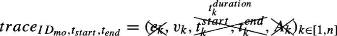
• We restrict MiSTA’s input data to consist solely of sequences of items rather than sequences of itemsets, because SITM assumes that a MO can not be present in multiple symbolic spatial entities at the same time. As a consequence, only extension projections will take place during MiSTA’s execution, and not enlargement ones. This assumption does not induce any changes in the MiSTA algorithm itself.

• Instead of attributing each temporal annotation to the transition between two consecutive items, we attribute it to the duration of stay in the first item, which represents the spatial entity of departure. This assumption simply serves to correct the interpretation of TASs according to the SITM.

Under these three assumptions, a short trajectory part, composed of tuples 4, 5, and 6 of the trajectory trace example used in Section 4.2, is transformed into the following TAS part:

S = <..., “N-1:P”, “D-1:EH”, “D-1:APOE”, ...>

A = <..., 60, 120, 240, ...>

where temporal annotations in A are expressed in seconds.

For τ= 20, the above TAS $(S, A) = \overset {60}{\textit {``N-1:P"}} \rightarrow \overset {120}{\textit {``D-1:EH"}} \rightarrow \overset {240}{\textit {``D-1:APOE"}}$τ-contains the TAS pattern $(S_{1}, A_{1}) = \overset {130}{\textit {``D-1:EH"}} \rightarrow \overset {255}{\textit {``D-1:APOE"}}$, but not the TAS pattern $(S_{2}, A_{2}) = \overset {150}{\textit {``D-1:EH"}} \rightarrow \overset {240}{\textit {``D-1:APOE"}}$, because their corresponding annotations differ by more than 20 seconds in at least one case.

Extracting Louvre visitor trajectory patterns

Before the actual mining process, we need to first pre-process the original trajectory dataset and tranform it into TAS form. First, we filter out any zone detection record with duration equal to 0. This leads to the deletion of 2,135 out a total of 20,245 records. Secondly, in 1,080 of those cases, the previous and the subsequent (to the deleted one) zones actually coincide, which constitutes further indication that the deleted zones are indeed errors. We merge those into a single zone in order to avoid any identical items appearing consecutively in the input TASs. Thirdly, we filter out all trajectories containing less than 3 zones. We opt for a low threshold value, taking into account the coarse spatiotemporal granularity of the available trajectory data, as well as their length distribution being left-skewed (Fig. 3). Finally, even though SITM can represent temporal gaps in the trajectories, MiSTA does not allow for gaps in the sequences. Therefore, we need to either erase all periods of visitor non-detection, or assume that the visitor is actually continuously located in the last known zone until he is re-detected in a different one. Given that the duration values are on the low side of what would normally be expected for a museum, we adopt the second approach as more realistic.

Next, in order to choose a proper τ parameter value, we calculate the normal distribution of the zone detection duration value. As expected and confirmed by the curve’s push to the right (Fig. 13), taking into account the detection gaps in the original trajectory dataset increases the values of the temporal annotations in MiSTA’s input TAS dataset. After trying out lower (i.e. stricter) and higher (i.e. more relaxed) values, we opted for τ= 117 sec, equal to the median zone stay duration value. In practice, this means that MiSTA will count a projected pattern’s occurrence in the input TAS data only as long as all of the corresponding annotations differ by less than 2 minutes.

Fig. 13

Normal distribution of the Louvre visitors’ duration of stay in each zone, under two different interpretations of the detection gaps

Table 3 contains the frequent TAS patterns of length equal to 3, enabling us to derive additional insight compared to the purely sequential approach of Section 4.3. Interestingly, all four patterns involve two types of movement taking place in two different parts of the museum, both characterized by a floor-switching back and forth type of behavior. In addition, they do not take place in the busiest parts of the museum like the ones identified in Section 4.3, which means that their support values are not much higher than their τ-support values. However, due to the fact that MiSTA involves a lossy step of merging frequent annotation intervals, we do not report any specific τ-support values because there is no approximation guarantee other than their being higher than supp_min= 5%. Instead, we include the contiguous sequence support which corresponds to requiring direct transitions only. We notice that the two patterns in the Arts décoratifs européens and Sculptures France Marly zones of the Richelieu wing (“R + 1:ADE” and “R0:SFM”) are almost always contiguous, whereas the two patterns in the Antiquités Égyptiennes zones of the Sully wing (“S0:AE” and “S + 1:AE”) more often include intermediate transitions. Also interestingly, the former two patterns contain more restricted duration intervals than the latter two, which suggests that visitors spend a more specific amount of time in that part of the Richelieu wing. Further interpretation of the reported time intervals is outside the scope of this illustrative experiment.

Table 3 The four frequent Louvre TAS patterns of length 3, for supp_min= 5% and τ= 117sec

Finally, we report on a few important implementation details. First, MiSTA counts each TAS pattern only once per input TAS, even when it appears multiple times in the same input TAS. In some application cases, this may not be the most desired way to calculate τ-support, particularly true for datasets containing long episodic trajectories. Secondly, as already explained, due to how τ-containment is defined [24], the TAS patterns reported by MiSTA are not necessarily contiguous. In such case, the corresponding annotation describes how long the visitor stayed in all of the zones combined, leading up to the next zone in the pattern. Again, a contiguous variation may be interesting depending on the case. Thirdly, since MiSTA’s annotations were originally designed to describe the transitions and the last item of each TAS is not followed by any transition, the duration of stay in the last zone of any trajectory is lost during its transformation to an input TAS. Technically, this issue can be easily solved by adding an “EXIT” item at the end of each TAS. This does not alter the mining output, apart from adding any frequent trajectory-ending patterns that contain the newly included interval.

5.3 Towards a SITM-based multidimensional temporally annotated sequential pattern mining algorithm

Different Big Data sources can be used to enrich trajectories with complex and heterogeneous semantic information [33]. In such cases, a sequential pattern mining problem becomes multidimensional, as illustrated in Section 5.1 for the case of semantic indoor trajectories. The few existing MDS pattern mining algorithms [12] all share a major limitation with respect to mobility data applications: they ignore the temporal dimension of the data.

On the other hand, as illustrated in Section 5.2, MiSTA is one of the few sequential pattern mining algorithms that does take time into account, but it does not account for multidimensional sequences.

Therefore, we detail hereafter several important characteristics of trajectories, as defined by SITM in Section 3, that are ignored by existing pattern mining algorithms:

• 1. The semantic content: MiSTA does not consider multidimensional items or any other type of contextual sequences, and therefore cannot use the semantic annotation sets A_traj and A_i, i ∈ [1,n] representing the semantic information of the trajectories and their parts.

• 2. The hierarchy of spatial regions: MiSTA does not consider any item hierarchy, and therefore cannot use the layered multigraph G=(V,E) representing the hierarchical indoor space.

• 3. The indoor space topology: MiSTA as well as all MDS pattern mining algorithms do not consider any topological or other type of network, and therefore cannot use the edges e_i representing the connections traversed by the MO in the accessibility NRG G_i=(V_i,E_acc,i) in any layer 0 ≤ i ≤ m of the hierarchy.

• 4. The starting time of each trajectory: MiSTA only considers time durations and not absolute timestamps, and therefore does not consider any of the beginning or ending timestamps $t^{start}_{i}$, $t^{end}_{i}$ contained in each presence interval i ∈ [1,n] and representing precisely when the MO entered/exited the spatial region.

The first two limitations can be addressed by combining MDS pattern mining with TAS pattern mining. The other two limitations can only be addressed if additional modeling elements are used within the mining process.

With respect to the first limitation, SITM can support the development of a combination of the two algorithmic approaches, allowing the extraction of multidimensional trajectory patterns. This provides a way to analyze the semantic aspects of trajectories as additional item dimensions, and can be accomplished by combining the time-aware prefix-projection generation mechanism of the MiSTA algorithm [24] with the multidimensional item generation mechanism of the M³SP algorithm [51] which is based on the notion of item specificity as explained in Section 5.1. In this regard, SITM’s semantic annotation sets A_i, specific to each presence interval i ∈ [1,n], can serve as analysis dimensions $\mathcal {D_{A}}$ [51] appearing in the frequent patterns’ items and even being associated with semantic hierarchies as discussed in Section 4.2. This is just one way of defining multidimensional trajectory pattern mining algorithms. Alternatively, a different time restriction scheme could be implemented over an existing MDS pattern mining method, thus providing proper temporal criteria for keeping or pruning the candidate multidimensional sequences.

With respect to the second limitation and in close connection to the first one, the set of cells V in SITM’s graph representation of the indoor space G=(V,E) can be set as the primary analysis dimension of the M³SP algorithm [51]. This can readily enable the mining of multidimensional trajectory sequences containing several levels of spatial hierarchy (in addition to any other semantic hierarchy).

With respect to the third limitation, SITM’s accessibility edges e_i can be used as topological restrictions for determining the validity (or plausibility) of candidate trajectory patterns. Such mechanism can be based for instance on the calculation of a proximity measure, as in the TP algorithm [17], which to our knowledge is the only sequential pattern mining algorithm to consider topological information. Doing so is not only interesting in terms of output quality, thanks to the resulting patterns respecting the indoor environment, but also as a speed-up technique since it serves as an additional pruning criterion. This is very important in a Big Data context, where large amounts of trajectories are quickly gathered and may even need to be mined in real-time.

With respect to the fourth limitation, SITM’s absolute timestamps $t^{start}_{i}$, $t^{end}_{i}$ specific to each presence interval i ∈ [1,n] can be used to enrich the temporal context of trajectories, and distinguish for example between the same visiting pattern occurring early in the day rather than late at night, or on Monday rather than on Friday, etc. In practice, quantizing the temporal dimension according to application needs and handling it as an additional analysis dimension, is the simplest way to introduce this temporal context in the mining process of multidimensional sequences.

As a first step to surmount the above limitations, we combine the approaches of MDS pattern mining and TAS pattern mining. Thus, we define a multidimensional temporally annotated sequence (MD-TAS) as a couple (s,α) consisting of two sequences:

• 1. An n-long sequence s =< s₁,s₂,...,s_n> of temporally ordered (according to a relation <_t) elementary vectors s_i = (c_i,1,c_i,2,...,c_i,m), i ∈ [1,n] whose components are itemsets c_i,j, j ∈ [1,m] composed of one or more items that respectively belong to dimensions $\mathcal {D} = \{D_{1}, D_{2}, ..., D_{m}\}$ in a specific position within their respective domain’s hierarchy ${\mathscr{H}} = \{H_{1}, H_{2}, ..., H_{m}\}$.

• 2. An n-long sequence α =< α₁,α₂,...,α_n> of real-valued temporal annotations, representing the duration of the respective vectors of s.

Hence, a MD-TAS can be represented as: $(s, \alpha ) = \overset {\alpha _{1}}{s_{1}} \rightarrow \overset {\alpha _{2}}{s_{2}} \rightarrow ... \rightarrow \overset {\alpha _{n}}{s_{n}}$

Moreover, an n-long MD-TAS T₁ = (s,α) is mdτ-contained (i.e. multidimensionally τ-contained) within another $n^{\prime }$-long MD-TAS $T_{2} = (s^{\prime }, \alpha ^{\prime })$, $n \leq n^{\prime }$ (T₁ ≼_mdτT₂) iff $\exists 0 \leq i_{0} < ... < i_{n} \leq n^{\prime }$ such that:

• 1. ∀_0≤k≤n: $s_{k} \leq _{{\mathscr{H}}} s^{\prime }_{i_{k}}$ ⇔ $c_{k,1} \leq _{H_{1}} c^{\prime }_{i_{k},1}, c_{k,2} \leq _{H_{2}} c^{\prime }_{i_{k},2}, ..., c_{k,m} \leq _{H_{m}} c^{\prime }_{i_{k},m}$

• 2. ∀_0≤k≤n: $|\alpha _{k} - \alpha ^{\prime }_{*k}| \leq \tau$ where $\alpha ^{\prime }_{*k} = \sum \limits _{j=i_{k-1}}^{i_{k}}$ $\alpha ^{\prime }_{j}$

Simply put, T₁ ≼_mdτT₂ holds when there is a (potentially non-contiguous) subsequence of T₂, whose itemsets correspond to all the itemsets of T₁ but are more general than them (condition 1), and whose annotations all differ by at most τ (condition 2) from the corresponding annotations in T₁.

Consequently, we define the multidimensional temporally annotated sequential (MD-TAS) pattern mining problem as follows: given as input a set of MD-TASs D_in, a minimum support value minsup, and a temporal relaxation value τ, return as output all frequent MD-TAS patterns that are mdτ-contained in D_in with a frequency higher than minsup.

Based on the previous problem definition and our proposed conceptual trajectory model defined in Section 3, we define the semantic indoor trajectory (SIT) pattern mining problem as follows: given as input a set of SITs T_in defined according to SITM, a minimum support value minsup, and a temporal relaxation value τ, return as output all frequent SIT patterns that are mdτ-contained in T_in with a frequency higher than minsup.

In this context, a SIT $T_{ID_{mo},t_{start},t_{end}} = (trace_{ID_{mo},t_{start},t_{end}}, A_{traj})$ with $trace_{ID_{mo},t_{start},t_{end}} = (e_{i},v_{i},t^{start}_{i},t^{end}_{i},A_{i})_{i \in [1,n]}$ can be formulated as a MD-TAS (s,α) where:

• the set of dimensions $\mathcal {D} = \{D_{space}, D_{semantics}\}$ contains a spatial dimension D_space which takes its values from the active domain of the edge-node couples (e_i,v_i) present in the indoor space graph G, and one or more semantic dimensions $D_{semantics} = \{D_{sem_{1}}, D_{sem_{2}}, ..., D_{sem_{m}}\}$ which take their values from the case-specific sets A_traj of whole-trajectory semantic annotations and from the sets A_i of trajectory-part semantic annotations.

• the corresponding set of hierarchies ${\mathscr{H}} = \{$G(V,E),H_semantics} contains a spatial hierarchy which is the indoor space graph, and one or more semantic taxonomies.

• the elementary vectors s_i = (e_i,v_i,A_i,1,...,A_i,m), i ∈ [1,n] contain the following items: a tuple (e_i,v_i), where the edge e_i represents the transition from node v_i− 1 to node v_i, and one or more items that respectively belong to dimensions $D_{semantics} = \{D_{sem_{1}}, D_{sem_{2}}, ..., D_{sem_{m}}\}$ in a specific position within the respective semantic hierarchy $H_{semantics} = \{H_{sem_{1}}, H_{sem_{2}}, ..., H_{sem_{m}}\}$.

• the annotation sequence $\alpha = < (t_{end_{1}}-t_{begin_{1}}), (t_{end_{2}}-t_{begin_{2}}), ..., (t_{end_{n}}-t_{begin_{n}}) {>}$ is extracted from subtracting the real-valued timestamps representing the start and finish of the corresponding elementary vectors of s.

• the absolute timestamps $t^{start}_{i},t^{end}_{i}$ can (optionally) be used in one of the m semantic dimensions, called $D_{sem_{temp}}$, to represent the temporal context.

Finally, there exist parallel pattern mining techniques for managing large volumes of data [4, 7, 44]. If trajectories are represented using SITM or any other sequence-based model, then a subset of those techniques relevant to sequential pattern mining [23] becomes particularly interesting in the Big Trajectory Data context. Typically, such techniques distribute the dataset in order to perform the counting step in parallel, although the candidate search space may also be split instead [7]. It actually depends on the specific dataset and the specific computing framework, which approach is most suitable, due to factors such as load balancing and communication costs. Even the type of method plays an important role as for example pattern growth methods have smaller memory footprints than candidate generation methods [4]. For example, sub-datasets of very different structure may be formed and cause some of the locally executed pattern mining methods to suffer in terms of computational cost. For instance, the MiSTA algorithm [24] used in Section 5.2 is very sensitive with respect to the length of the input TASs, which is why the trajectory dataset needs to be carefully split. Alternatively, the search space can be split thanks to the prefix-projection exploration mechanism.

6 Conclusions and future work

In this work, we introduced a new model for representing semantic trajectories in indoor environments, SITM, based on an indoor space representation compatible with the IndoorGML standard [38] and using a hierarchical graph structure similar to [31]. Our indoor space representation differs mainly in that it requires a static hierarchy of three basic layers (building, floor, room) and proposes two more typical layers (building complex, intra-room region of interest), thus avoiding ad-hoc subdivisions of space. Over this space representation, we introduced a semantic indoor trajectory model called SITM, by coupling each visitor’s sequences of presence intervals in symbolic indoor areas, with semantic annotations and flexible concept definitions.

Motivated by our case study involving a mobility dataset of Louvre visitors, composed of spatially aggregated timestamped detections, we instantiated the model and offered trajectory examples illustrating how its expressiveness can be exploited. We also ran experiments using existing standard and advanced pattern mining methods, in order to qualitatively study them, but also to illustrate how new trajectory pattern mining methods can combine multiple data dimensions with a temporal dimension, and provided a formalization for the problem of trajectory mining represented under SITM.

As future work, it would be interesting to integrate more thoroughly the indoor space representation with formal ontologies of cultural heritage information (e.g. CIDOC Conceptual Reference Model [19]). Also, modeling virtual instead of physical trajectories could be compelling in the museum domain, where an attention-based interpretation of visitor movement can be even more important than one based on physical presence. Furthermore, with respect to the analysis of semantic trajectories, we plan to implement our proposal of combining the temporal and multidimensional aspects of sequential pattern mining methods, also adding topological information in the mining process, in order to derive interesting indoor mobility behaviors. Also, we plan to test parallel versions of our algorithms in order to scale up the analysis. With regards to the Louvre case in particular, it is interesting to account for the problem of data sparsity by restructuring longer indicative visits from the actual fragmented zone sequences.

References

Afyouni I, Ray C, Claramunt C (2012) Spatial models for context-aware indoor navigation systems: A survey. J Spat Inf Sci 1(4):85–123
Afyouni I, Ray C, Claramunt C (2017) Representation: indoor spaces. Am Cancer Soc, 1–12
Alvares LO, Bogorny V, Kuijpers B, de Macedo JAF, Moelans B, Vaisman A (2007) A model for enriching trajectories with semantic geographical information. In: Proceedings of the 15th annual ACM international symposium on advances in geographic information systems. GIS ’07. ACM, pp 22:1–22:8
Anastasiu DC, Iverson J, Smith S, Karypis G (2014) Big data frequent pattern mining. Springer International Publishing, Cham, pp 225–259
Andrienko G, Andrienko N, Bak P, Keim D, Kisilevich S, Wrobel S (2011a) A Conceptual Framework and Taxonomy of Techniques for Analyzing Movement. J Vis Lang Comput 22(3):213–232
Andrienko G, Andrienko N, Heurich M (2011b) An event-based conceptual model for context-aware movement analysis. Int J Geogr Inf Sci 25:1347–1370
Apiletti D, Baralis E, Cerquitelli T, Garza P, Pulvirenti F, Venturini L (2017) Frequent itemsets mining for big data: a comparative analysis. Big Data Res 9:67–83
Becker T, Nagel C, Kolbe TH (2009) Supporting contexts for indoor navigation using a multilayered space model. In: 2009 Tenth international conference on mobile data management, systems, services and middleware, pp 680–685
Bogorny V, Heuser CA, Alvares LO (2010) A conceptual data model for trajectory data mining. In: Proceedings of the 6th international conference on geographic information science (GIScience’10). Lecture Notes in Computer Science. Springer, Berlin, pp 1–15
Bogorny V, Renso C, de Aquino AR, de Lucca Siqueira F, Alvares LO (2014) CONSTAnT - A conceptual data model for semantic trajectories of moving objects. Trans GIS 18(1):66–88
Brumitt B, Shafer S (2001) Topological world modeling using semantic spaces. In: UbiComp 2001 workshop on location modeling for ubiquitous computing, pp 55–61
Bu Daher J, Brun A, Boyer A (2018) A review on heterogeneous multi-source and multi-dimensional data mining. Technical report, LORIA - Universite de Lorrainé
Chen J, Cohn AG, Liu D, Wang S, Ouyang J, Yu Q (2015) A survey of qualitative spatial representations. Knowl Eng Rev 30(1):106–136
Cohn A, Bennett B, Gooday J, Gotts M (1997) Qualitative spatial representation and reasoning with the region connection calculus. GeoInformatica 1:275–316
Cruz C (2017) Semantic trajectory modeling for dynamic built environments. In: Special session on environmental and geo-spatial data analytics (EnGeoData 2017), The 4th IEEE international conference on data science and advanced analytics, Tokyo, Japan
Cui Z, Cohn AG, Randell DA (1993) Qualitative and topological relationships in spatial databases. In: Proceedings of the third international symposium on advances in spatial databases (SSD ’93). Lecture Notes in Computer Science. Springer, Berlin, pp 296–315
Devitt A, Duffin J, Moloney R (2005) Topographical proximity for mining network alarm data. In: Proceedings of the 2005 ACM SIGCOMM workshop on mining network data, association for computing machinery, New York, NY, USA, MineNet ’05, pp 179–184
Diakité A, Zlatanova S, Li KJ (2017) About the subdivision of indoor spaces in IndoorGML. In: 12th 3D Geoinfo conference, pp 41–48
Doerr M, Ore CE, Stead S (2007) The CIDOC conceptual reference model - a new standard for knowledge sharing. In: Tutorials, posters, panels and industrial contributions at the 26th international conference on conceptual modeling,. ER ’07. Australian Computer Society, Inc., pp 51–56
Egenhofer M, Herring J (1992) categorizing binary topological relations between regions, lines and points in geographic databases. The 9-Intersection Formalism and Its Use For Natural-Language Spatial Predicates, 94:1–28
Egenhofer MJ (1991) Reasoning about binary topological relations. In: Proceedings of the second international symposium on advances in spatial databases. SSD ’91. Springer, London, pp 143–160
Egenhofer MJ, FR D (1991) Point-set topological spatial relations. Int J Geogr Inf Syst 5(2):161–174
Gan W, Lin JCW, Fournier-Viger P, Chao HC, Yu PS (2019) A survey of parallel sequential pattern mining. ACM Trans Knowl Discov Data 13(3)
Giannotti F, Nanni M, Pedreschi D, Pinelli F (2006) Mining sequences with temporal annotations. In: Proceedings of the ACM symposium on applied computing, vol 1, pp 593–597
Giannotti F, Nanni M, Pinelli F, Pedreschi D (2007) Trajectory pattern mining. In: Proceedings of the 13th ACM SIGKDD International conference on knowledge discovery and data mining. KDD ’07. ACM, New York, pp 330–339
Han J, Pei J, Yin Y, Mao R (2004) Mining Frequent Patterns without Candidate Generation: A Frequent-Pattern Tree Approach. Data Min Knowl Disc 8(1):53–87
Harbelot B, Arenas H, Cruz C (2015) LC3: a spatio-temporal and semantic model for knowledge discovery from geospatial datasets. J Web Semant 35:3–24. geospatial Semantics
Hirtle SC, Jonides J (1985) Evidence of hierarchies in cognitive maps. Mem Cognit 13(3):208–217
Hu H, Lee DL (2004) Semantic location modeling for location navigation in mobile environment. In: 5th IEEE international conference on mobile data management (MDM 2004), 19-22 January, vol 2004. IEEE Computer Society, Berkeley, pp 52–61
Jensen CS, Lu H, Yang B (2010) Indoor - a new data management frontier. IEEE Comput Soc Data Eng Bull 33(2):12–17
Kang HK, Li KJ (2017) A standard indoor spatial data model - OGC IndoorGML and implementation approaches. ISPRS Int J Geoinf 6(4):1–25
Kivelä M, Arenas A, Barthelemy M, Gleeson JP, Moreno Y, Porter MA (2014) Multilayer networks. J Complex Netw 2(3):203–271
Kong X, Li M, Ma K, Tian K, Wang M, Ning Z, Xia F (2018) Big trajectory data: a survey of applications and services. IEEE Access 6:58295–58306
Kuflik T, Dim E (2019) Integrating signals for reasoning about visitors’ behavior in cultural heritage. In: Alameda-Pineda X, Ricci E, Sebe N (eds) Multimodal behavior analysis in the wild. Computer Vision and Pattern Recognition. Academic Press, pp 159–169
Le Boeuf P, Doerr M, Ore CE, Stead S (2019) Definition of the CIDOC conceptual reference model. http://www.cidoc-crm.org/Version/version-6.2.6, accessed on 05.05.2020
Lee J (2004) A spatial access-oriented implementation of a 3-D GIS topological data model for urban entities. Geoinformatica 8(3):237–264
Lee J, Li KJ, Zlatanova S, Kolbe TH, Nagel C, Becker T (2010) Requirements and space-event modeling for indoor navigation. Tech. rep., Open Geospatial Consortium
Lee J, Li KJ, Zlatanova S, Kolbe TH, Nagel C, Becker T (2018) OGC IndoorGML. Tech. rep., Open Geospatial Consortium
Louvre Museum Press Room (2018) 10.2 million visitors to the Louvre in 2018. https://presse.louvre.fr/10-2-million-visitors-to-the-louvre-in-2018/, accessed on 05.05.2020
Louvre Museum Press Room (2019) 9.6 million visitors to the Louvre in 2019. https://presse.louvre.fr/9-6-million-visitors-to-thebr-louvre-in-2019/, accessed on 05.05.2020
Louvre Museum Press Room (2020) 1.1 million visitors for “Leonardo da Vinci” A new record for an exhibition at the Louvre. https://presse.louvre.fr/1-1-million-visitors-for-leonardo-da-vincibr-a-new-record-for-an-exhibitionnbspat-the-louvre/https://presse.louvre.fr/1-1-million-visitors-for-leonardo-da-vincibr-a-new-record-for-an-exhibitionnbspat-the-louvre/, accessed on 05.05.2020
Lu H, Guo C, Yang B, Jensen CS (2016) Finding frequently visited indoor POIs using symbolic indoor tracking data. In: Proceedings of the 19th international conference on extending database technology (EDBT2016), pp 449–460
Mello R d S, Bogorny V, Alvares LO, Santana LHZ, Ferrero CA, Frozza AA, Schreiner GA, Renso C (2019) MASTER: A Multiple Aspect View on Trajectories. Trans GIS 23(4):805–822
Moens S, Aksehirli E, Goethals B (2013) Frequent Itemset mining for big data. In: 2013 IEEE international conference on big data, pp 111–118
Parent C, Spaccapietra S, Renso C, Andrienko G, Andrienko N, Bogorny V, Damiani ML, Gkoulalas-Divanis A, Macedo J, Pelekis N, Theodoridis Y, Yan Z (2013) Semantic trajectories modeling and analysis. ACM Comput Surv 45(4):42:1–42:32
Pei J, Han J, Mortazavi-Asl B, Pinto H, Chen Q, Dayal U, Hsu MC (2001) PrefixSpan: mining sequential patterns efficiently by prefix-projected pattern growth. In: Proceedings of the 17th international conference on data engineering. IEEE Computer Society, USA, pp 215–224
Peuquet DJ (2002) Representations of space and time. Guilford Press, New York
Pinto H, Han J, Pei J, Wang K, Chen Q, Dayal U (2001) Multi-dimensional sequential pattern mining. In: Proceedings of the tenth international conference on information and knowledge management. CIKM ’01. ACM, New York, pp 81–88
Plantevit M, Choong YW, Laurent A, Laurent D, Teisseire M (2005) M2SP: Mining sequential patterns among several dimensions. In: Jorge AM, Torgo L, Brazdil P, Camacho R, Gama J (eds) Knowledge discovery in databases: PKDD 2005, vol 3271. Springer, Berlin, pp 205–216
Plantevit M, Laurent A, Teisseire M (2006) HYPE: mining hierarchical sequential patterns. In: Proceedings of the 9th ACM international workshop on data warehousing and OLAP. DOLAP ’06. ACM, New York, pp 19–26
Plantevit M, Laurent A, Laurent D, Teisseire M, Choong YW (2010) Mining multi-dimensional and multi-level sequential patterns. ACM Transactions on Knowledge Discovery from Data (TKDD) 4:1–37
Popa IS, Zeitouni K, Oria V, Kharrat A (2015) Spatio-temporal compression of trajectories in road networks. GeoInformatica 19(1):117–145
Renz J (2002) Qualitative spatial reasoning with topological information. Springer, Berlin
Spaccapietra S, Parent C (2011) Adding meaning to your steps. In: Proceedings of the 30th international conference on conceptual modeling. ER’11. Springer, Berlin, pp 13–31
Spaccapietra S, Parent C, Damiani ML, de Macedo JA, Porto F, Vangenot C (2008) A conceptual view on trajectories. Data Knowl Eng 65(1):126–146
Srikant R, Agrawal R (1996) Mining sequential patterns: generalizations and performance improvements. In: Proceedings of the 5th international conference on extending database technology: advances in database technology. EDBT ’96. Springer, London, pp 3–17
Stoffel EP, Lorenz B, Ohlbach HJ (2007) Towards a semantic spatial model for pedestrian indoor navigation. In: Hainaut JL, Rundensteiner EA, Kirchberg M, Bertolotto M, Brochhausen M, Chen YPP, Cherfi SSS, Doerr M, Han H, Hartmann S, Parsons J, Poels G, Rolland C, Trujillo J, Yu E, Zimányie E (eds) Advances in conceptual modeling – foundations and applications. Springer, Berlin, pp 328–337
Stoffel EP, Schoder K, Ohlbach HJ (2008) Applying hierarchical graphs to pedestrian indoor navigation. In: Proceedings of the 16th ACM SIGSPATIAL international conference on advances in geographic information systems. GIS ’08. ACM, New York, pp 54:1–54:4
Villalonga C, Razzaq MA, Khan WA, Pomares H, Rojas I, Lee S, Banos O (2016) Ontology-based high-level context inference for human behavior identification. Sensors 16(10):1–26
Xu J, Lu H, Güting RH (2019) Understanding human mobility: A multi-modal and intelligent moving objects database. In: Proceedings of the 16th international symposium on spatial and temporal databases, association for computing machinery, New York, NY, USA, SSTD ’19, pp 222–225
Yan Z, Macedo J, Parent C, Spaccapietra S (2008) Trajectory ontologies and queries. Trans GIS 12(s1):75–91
Yan Z, Parent C, Spaccapietra S, Chakraborty D (2010) A hybrid model and computing platform for spatio-semantic trajectories. In: The semantic web: research and applications. Lecture Notes in Computer Science, vol 6088. Springer, Berlin, pp 60–75
Yan Z, Chakraborty D, Parent C, Spaccapietra S, Aberer K (2011) SeMiTri: a framework for semantic annotation of heterogeneous trajectories. In: Proceedings of the 14th international conference on extending database technology. EDBT/ICDT ’11. ACM, New York, pp 259–270
Yan Z, Chakraborty D, Parent C, Spaccapietra S, Aberer K (2013) Semantic Trajectories: Mobility Data Computation and Annotation. ACM Trans Intell Syst Technol 4(3):49,1–49,38
Yoshimura Y, Krebs A, Ratti C (2017) Noninvasive bluetooth monitoring of visitors’ length of stay at the Louvre. IEEE Pervasive Comput 16(2):26–34
Yoshimura Y, Sinatra R, Krebs A, Ratti C (2019) Analysis of visitors’ mobility patterns through random walk in the Louvre Museum. J Ambient Intell Humaniz Comput
Zheng K, Su H (2015) Go Beyond Raw Trajectory Data: Quality and Semantics. IEEE Data Eng Bull 38(2):27–34
Acknowledgements
The authors would like to thank Anne Krebs for her multifaceted help and Mohamed Boudjemaa Hamici for his contributions in developing the code for the results presented in Table 2.
This work was supported by the TRAJECTOIRES project funded by the Paris Seine Graduate School Humanities, Creation, Heritage, Investissement d’Avenir ANR-17-EURE-0021 – Foundation for Cultural Heritage Science.
Karine Zeitouni’s work in this paper was supported by the MASTER project that has received funding from the European Union’s Horizon 2020 research and innovation programme under the Marie-Slodowska Curie grant agreement N. 777695.
Author information
Authors and Affiliations
Corresponding author
Additional information
Publisher’s note
Springer Nature remains neutral with regard to jurisdictional claims in published maps and institutional affiliations.
Rights and permissions
About this article
Cite this article
Kontarinis, A., Zeitouni, K., Marinica, C. et al. Towards a semantic indoor trajectory model: application to museum visits. Geoinformatica 25, 311–352 (2021). https://doi.org/10.1007/s10707-020-00430-x
Received:
Revised:
Accepted:
Published:
Issue Date:
DOI: https://doi.org/10.1007/s10707-020-00430-x