A Novel Continuous Nonsingular Finite–Time Control for Underwater Robot Manipulators

Abstract

In this paper, the tracking control problem of underwater robot manipulators is investigated under the influence of the lumped disturbances, including unknown ocean current disturbances and parameter uncertainties. The proposed novel continuous nonsingular finite–time (CNFT) control method is twofold. Firstly, the modified adaptive super–twisting algorithm (ASTA) is proposed with a nonsingular fast terminal sliding mode (NFTSM) manifold to guarantee the finite–time convergence both in the sliding mode phase and the reaching phase. Secondly, a higher–order super–twisting disturbance observer (HOSTDO) is exploited to attenuate the effects of the lumped disturbances. Considering the time–varying gain matrix of the closed–loop control system, the bounded stability is strictly proved via the Lyapunov theory. Hence, the superiority of the proposed controller is singularity–free, fast convergence, chattering–free, high steady–state tracking performance, and good robustness by resorting to the methods of CNFT control and ASTA in combination with a disturbance observer. Finally, numerical simulations are conducted on a two degree–of–freedom (DOF) underwater robot manipulator to demonstrate the effectiveness and high tracking performance of the designed controller.

1. Introduction

The last few decades have seen giant undersea technological improvements on underwater robot manipulators in many scientific fields, such as oceanographic observation, sub–sea detection, and some military applications [1]. Considering the complex underwater circumstances, it is quite difficult to complete tasks with high control precision and a fast dynamic response [2]. Hence, the impact of the hydrodynamic forces, such as drag torques and buoyancy torques, should be considered [3]. Minglu Zhang et al. performed the modeling analysis and the simulation of a viscous hydrodynamic model of single–DOF underwater manipulators [4]. In addition, the hydrodynamic regulation was analyzed for underwater manipulators [5]. However the tracking problem was not included. Considering the roughly modeled hydrodynamics, some robust control strategies have been proposed for underwater manipulators in the last few decades to achieve satisfactory tracking performance. A proportional–integral–derivative (PID) control scheme was designed for the underwater cable–driven hyper–redundant manipulator, which experimentally achieved underwater grasping and load carrying [6]. A model–reference adaptive control was proposed for a hydrodynamic underwater manipulator to deal with the nonlinear dynamics and hydrodynamics [7]. Besides, sliding mode control was designed for the underwater manipulator but the hydrodynamic effect was only regarded as the external disturbances [8]. However, the robustness and the precision can not be ensured at the same time. In 2020, an adaptive sliding mode control was proposed for the underwater manipulator to achieve finite time tracking with the asymmetric saturation [9]. Chao Yang et al. combined the adaptive control, sliding mode and PID control to address the joint tracking control problem [10]. However, the proposed sliding mode controllers still suffer from the chattering problem, which decreases tracking performance. Hence, it is still a great challenge to obtain high precision and strong robustness tracking results.

Sliding mode (SM) control has been wildly considered in many nonlinear systems with significant uncertainties [11]. In recent years, different kinds of sliding mode control, including robust sliding mode control [12], multiple sliding mode control [13], and dynamic sliding mode control [14], have been widely investigated. Specially, the nonsingular fast terminal sliding mode (NFTSM) control was proposed to achieve fast convergence and singularity–free at the same time [15,16,17]. However, the discontinuous nature of the control law always leads to an undesirable chattering problem [18]. Thus the higher–order SM (HOSM) method was proposed to reduce the chattering effect [19,20]. The core idea of HOSM control is to design a continuous sliding variable which is differentiable up to the higher order, so as to ensure the continuity of control signals [21]. In the SM control community, the super–twisting algorithm (STA) is one of the most effective HOSM techniques to achieve a high control accuracy [22,23]. However, these control methods require the prior information of the lumped disturbances, which is not easily accessible for the underwater robot manipulator system in a submarine environment. In order to tackle this problem, the adaptive method for the switching function, which is known as adaptive STA (ASTA), can be used [24,25].

Although TSM control with STA can be demonstrated stable through strict Lyapunov theory [23], it is difficult to prove the stability when combining NFTSM control with STA because of the time–varying gain matrix. Some researches directly utilized STA to eliminate the chattering without strict proof [26], while others adopted an integral sliding surface to avoid this issue [27]. Therefore, it is meaningful to take the time–varying gain matrix into consideration when proving the stability of the control system through strict Lyapunov theory.

It is worth noting that the STA can also be used for system observation [28]. J. A. Moreno demonstrated the stability and robustness of a second–order super–twisting observer for a nonlinear system by using strict Lyapunov functions [29]. Besides, a super–twisting observer was proposed for a Stewart platform to solve the forward kinematics problem [30]. However, most of these super–twisting observers are used to estimate the state variables, and a minority of them are considered to approximate the lumped disturbances.

Motivated by the above mentioned studies, our target is to propose a novel CNFT control for the underwater robot manipulators. The contributions of our paper are concluded as follows: (1) A novel HOSTDO–based NFTSM control with the modified ASTA scheme is firstly proposed for the underwater robot manipulators considering the unknown lumped disturbances. It provides a new theoretical way to resolve the chattering problem, which is the main obstacle for the application of SM control. (2) The modified ASTA is formulated to reserve the merits of traditional STA while prior information of the lumped disturbances is not needed. Additionally, it has a faster convergence rate than the standard STA. (3) The disturbance attenuation is achieved through the HOSTDO, which can strongly improve robustness of the control system. (4) Considering the time–varying gain matrix due to the combination of NFTSM and modified ASTA, the corresponding closed–loop stability of the control system is strictly verified through the Lyapunov theory.

The rest of our paper is organized as follows. The dynamic model of the underwater robot manipulators and some fundamental facts are presented in Section 2. The detailed structural procedure of the control strategy is reported in Section 3. In Section 4, the proposed control is applied to a two–DOF underwater robot manipulator. The trajectory tracking performances are also compared with those of the other three controllers. Finally, concluding remarks are given in Section 5.

2. Problem Formulation

2.1. Underwater Robot Manipulator Model and Properties

The n–joint underwater robot manipulators can be described by the following Euler–Lagrange equation [31,32]:

$$M\left(q\right)\ddot{q}+C(q,\dot{q})\dot{q}+G\left(q\right)+{\tau }_w(q,\dot{q})={\tau }_{edis}+\tau$$

(1)

where $q,\dot{q},\ddot{q}\in R^n$ denote the position, velocity, and acceleration vectors of joints, respectively; $M\left(q\right)\in R^{n\times n}$, $C(q,\dot{q})\in R^{\mathrm{n}}$, $G\left(q\right)\in R^n$ are the inertia matrix, Coriolis/centrifugal matrix, and gravitational vector, respectively; ${\tau }_w(q,\dot{q})\in R^n$ denotes the hydrodynamic force vector, which contains drag torque ${\tau }_D$ and buoyancy torque ${\tau }_B$ and satisfies ${\tau }_w={\tau }_D+{\tau }_B$; ${\tau }_{edis}\in R^n$ is the unknown external disturbance vector; and $\tau \in R^n$ denotes the control input torque vector.

Assumption 1.

The model parameters can be partitioned into different parts which can be given as follows: $M\left(q\right)=M_0\left(q\right)+M_{\Delta }\left(q\right),C(q,\dot{q})=C_0(q,\dot{q})+C_{\Delta }(q,\dot{q}),G\left(q\right)=G_0\left(q\right)+G_{\Delta }\left(q\right),{\tau }_w(q,\dot{q})={\tau }_{w0}(q,\dot{q})+{\tau }_{w\Delta }(q,\dot{q})$, where $M_0\left(q\right)$, $C_0(q,\dot{q})$, $G_0\left(q\right)$, and ${\tau }_{w0}(q,\dot{q})$ are the nominal parts and $M_{\Delta }\left(q\right)$, $C_{\Delta }(q,\dot{q})$, $G_{\Delta }\left(q\right)$ and ${\tau }_{w\Delta }(q,\dot{q})$ denote the uncertain bounded parts.

Assumption 2.

The target trajectory and its derivatives $q_d,{\dot{q}}_d,{\ddot{q}}_d\in R^n$ are known and bounded.

To simplify the design and analysis of the proposed controller, we define $x_1=q$, $x_2=\dot{q}$, and considering Assumption 1, the dynamic model (1) can be rewritten as:

$$\begin{array}{cc}\hfill {\dot{x}}_1& =x_2\hfill \\ \hfill {\dot{x}}_2& ={M_0}^{-1}\left(x_1\right)u\left(t\right)+f(x_1,x_2)+\Delta (x_1,x_2,t)\hfill \\ \hfill y& =x_1\hfill \end{array}$$

(2)

where $f(x_1,x_2)={M_0}^{-1}\left[-C_0{x}_2-G_0-{\tau }_w\right]$, $u\left(t\right)=\tau$ is the time–varying control input, and $\Delta \in R^n$ represents the lumped disturbance vector which is defined as $\Delta (x_1,x_2,t)=M_0^{-1}\left[-M_{\Delta }{x}_2-C_{\Delta }{x}_2-G_{\Delta }-{\tau }_{w\Delta }+{\tau }_{edis}\right]$.

The control objective is to design a proper controller so that high tracking precision and fast convergence can be obtained without chattering and singularity problems.

Remark 1.

The fluid in the underwater circumstance should be irrational and unbounded, thus the rotation of the fluid could be very small compared with that of the rigid body.

Remark 2.

The added mass torque and the vortex influence are not considered in this paper. Considering the fact that the acceleration of the underwater manipulator body is always slow, the added mass torque and the vortex influence are small enough to be neglected in practical underwater robotic applications.

2.2. Fundamental Facts

Our control method will be accomplished based on some fundamental facts to achieve the finite–time convergence and system stability.

Definition 1.

For the sake of brevity and clarity, we define that $diag\left\{·\right\}\in R^{n\times n}$ stands for the positive definite diagonal matrix, and the vectors $sgn\left(\varsigma \right)\in R^n$ and ${\varsigma }^{\left[r\right]}\in R^n$ are as follows: $sgn\left(\varsigma \right)={\left[sign\left({\varsigma }_1\right),\cdots ,sign\left({\varsigma }_n\right)\right]}^T$, ${\varsigma }^{\left[r\right]}=\left[{\left|{\varsigma }_1\right|}^{r}sign\left({\varsigma }_1\right),\cdots ,\right.$${\left.{\left|{\varsigma }_n\right|}^{r}sign\left({\varsigma }_n\right)\right]}^T$, where $\varsigma ={\left[{\varsigma }_1,\cdots ,{\varsigma }_n\right]}^T\in R^n$ is the vector variable, $r>0$ stands for a known constant, and when $r\ge 1$, it can be verified that $\frac{d}{dt}{\varsigma }^{\left[r\right]}=r{\left|\varsigma \right|}^{r-1}\dot{\varsigma }$. Besides, $sign(·)$ is a standard symbolic function.

Definition 2.

The powers of error vectors are defined as:

$$\begin{array}{cc}\hfill e^{\left[\phi \right]}& ={\left[e_1^{\left[\phi \right]},\cdots ,e_n^{\left[\phi \right]}\right]}^T\in R^n\hfill \\ \hfill {\dot{e}}^{[l/p]}& ={\left[{{\dot{e}}_1}^{[l/p]},\cdots ,{{\dot{e}}_n}^{[l/p]}\right]}^T\in R^n\hfill \\ \hfill {\dot{e}}^{[2-l/p]}& ={\left[{{\dot{e}}_1}^{[2-l/p]},\cdots ,{{\dot{e}}_n}^{[2-l/p]}\right]}^T\in R^n\hfill \\ \hfill {\left|e\right|}^{\phi -1}& =diag\left\{{\left|e_1\right|}^{\phi -1},\cdots ,{\left|e_n\right|}^{\phi -1}\right\}\in R^{n\times n}\hfill \\ \hfill {\left|\dot{e}\right|}^{(l/p)-1}& =diag\left\{{\left|{\dot{e}}_1\right|}^{(l/p)-1},\cdots ,{\left|{\dot{e}}_n\right|}^{(l/p)-1}\right\}\in R^{n\times n}.\hfill \end{array}$$

(3)

Lemma 1

([33]). Considering a system described in (2), and any real numbers $a>0$ and $0<b<1$ so that the Lyapunov function $V\left(x\right)$ is positive definite and $\dot{V}\left(x\right)+a{V}^b\left(x\right)$ is negative semi–definite, the control system will be stable and all the signals will be bounded in finite time, and the settling time can be estimated by $T_0\le \frac{1}{a(1-b)}{V}^{1-b}\left(x_0\right)$.

3. The Design of CNFT Control Based on HOSTDO and ASTA

In this section, a novel CNFT control method based on ASTA is proposed for underwater manipulators. First, a NFTSM manifold is designed to be free from the singularity problem. Second, the modified STA is derived from the adaptive method to alleviate the chattering phenomenon and obtain good dynamical performance. Besides, the parameter adaptation method ensures that there is no need for prior information of the upper bound of the lumped disturbances. Finally, HOSTDO is utilized to estimate and compensate the lumped disturbances.

3.1. The Design of HOSTDO

STA is an important method for the control and the observation. The HOSTDO dynamics is given in the following form:

$$\begin{array}{cc}\hfill {\dot{\widehat{x}}}_1& ={\widehat{x}}_2+z_1\hfill \\ \hfill {\dot{\widehat{x}}}_2& ={\widehat{x}}_3+M_0^{-1}u+f+z_2\hfill \\ \hfill {\dot{\widehat{x}}}_3& ={\widehat{x}}_4+z_3\hfill \\ \hfill {\dot{\widehat{x}}}_4& =z_4\hfill \end{array}$$

(4)

where the state vectors are given as $x_3=\Delta (x_1,x_2,t)$, $x_4=\dot{\Delta }(x_1,x_2,t)$; ${\widehat{x}}_1$, ${\widehat{x}}_2$, ${\widehat{x}}_3$, ${\widehat{x}}_4$ are the estimations of state vectors $x_1$, $x_2$, $x_3$, $x_4$, respectively; and $z_1$, $z_2$, $z_3$, and $z_4$ are the correction terms. And for simplicity, the initial values of $z_1$, $z_2$, $z_3$, $z_4$ are assumed to be zero. Then we define the state estimate error variables ${\epsilon }_1=x_1-{\widehat{x}}_1$, ${\epsilon }_2=x_2-{\widehat{x}}_2$, ${\epsilon }_3=x_3-{\widehat{x}}_3$, and ${\epsilon }_4=x_4-{\widehat{x}}_4$. The correction terms are defined as $z_1={\xi }_1{{\epsilon }_1}^{\left[3/4\right]}$, $z_2={\xi }_2{{\epsilon }_1}^{\left[1/2\right]}$, $z_3={\xi }_3{{\epsilon }_1}^{\left[1/4\right]}$, $z_4={\xi }_{4}sgn\left({\epsilon }_1\right)$, in which ${\xi }_1$, ${\xi }_2$, ${\xi }_3$, and ${\xi }_4$ are positive constants.

Using (2), we obtain the observer dynamic error model as:

$$\begin{array}{cc}\hfill {\dot{\epsilon }}_1& =-{\xi }_1{{\epsilon }_1}^{\left[3/4\right]}+{\epsilon }_2\hfill \\ \hfill {\dot{\epsilon }}_2& =-{\xi }_2{{\epsilon }_1}^{\left[1/2\right]}+{\epsilon }_3\hfill \\ \hfill {\dot{\epsilon }}_3& =-{\xi }_3{{\epsilon }_1}^{\left[1/4\right]}+{\epsilon }_4\hfill \\ \hfill {\dot{\epsilon }}_4& =-{\xi }_{4}sgn\left({\epsilon }_1\right)+\ddot{\Delta }.\hfill \end{array}$$

(5)

By selecting the gains ${\xi }_1$, ${\xi }_2$, ${\xi }_3$, and ${\xi }_4$ according to [34], we can obtain that the proposed HOSTDO reaches finite–time stability and ${\epsilon }_i=0,i=1,2,3,4$, which implies ${\dot{\epsilon }}_i=0,i=1,2,3,4$. Then the estimates of disturbances are given as follows $\widehat{\Delta }=-{\xi }_2{{\epsilon }_1}^{\left[1/2\right]}+v_1,{\dot{v}}_1=-{\xi }_3{{\epsilon }_1}^{\left[1/4\right]}+v_2,{\dot{v}}_2=-{\xi }_{4}sgn\left({\epsilon }_1\right)$, where the initial value of $\widehat{\Delta }$, $v_1$, $v_2$ are supposed to be 0 for simplicity.

Remark 3.

The proposed disturbance observer generates a more smooth output to estimate and compensate the unknown lumped disturbances which can obviously alleviate the chattering issue. Furthermore, Equation (4) can be used to approximate the system state vectors in other research [35,36]. The convergence and robustness of the HOSTDO can be verified by Lyapunov theory, and the detailed proof can be referred to [34].

3.2. HOSTDO Based CNFT Control Design with ASTA Method and Time–Varying Gain Matrix

To ensure the chattering–free ability and eliminate the need for the prior information of the upper bound, the modified STA scheme is utilized with the parameter adaptation method to obtain good comprehensive performances. A novel HOSTDO–based CNFT control scheme with the ASTA method is proposed in this section.

Define the tracking error as $e=q-q_d$ with $q_d$ being the desired trajectory. To ensure the finite–time convergence ability and singularity–free performance, a NFTSM manifold is designed as [26]:

$$s=e+{\sigma }_1{e}^{\left[\phi \right]}+{\sigma }_2{\dot{e}}^{[l/p]}$$

(6)

where $s={\left[s_1,\cdots ,s_n\right]}^T\in R^n$ is the sliding vector; ${\sigma }_1$, ${\sigma }_2$ are the designed positive constants; l and p are positive odd numbers satisfying $1<l/p<2$; and $\phi$ is a designed constant satisfying $\phi >l/p$.

The derivative of (6) is:

$$\begin{array}{cc}\hfill \dot{s}& =\dot{e}+{\sigma }_1\phi {\left|e\right|}^{\phi -1}\dot{e}+{\sigma }_2\frac{l}{p}{\left|\dot{e}\right|}^{l/p-1}(\ddot{q}-{\ddot{q}}_d)\hfill \\ \hfill & =\dot{e}+{\sigma }_1\phi {\left|e\right|}^{\phi -1}\dot{e}+{\sigma }_2\frac{l}{p}{\left|\dot{e}\right|}^{l/p-1}({M_0}^{-1}\left(x_1\right)u+f(x_1,x_2)+\Delta (x_1,x_2,t)-{\ddot{q}}_d).\hfill \end{array}$$

(7)

It can be deduced from (7) that $\phi -1>0$ and $l/p-1>0$ are valid considering $1<l/p<2$ and $\phi >l/p$, so the singularity phenomenon can be avoided successfully. Meanwhile, the system’s dynamic convergence speed is enhanced by combining the merits of the NFTSM manifold.

According to the NFTSM manifold and adaptive modified STA scheme, the CNFT control law based on the HOSTDO is designed as:

$$u=u_{eq}+u_{re}$$

(8)

where

$$u_{eq}=M_0\left(x_1\right)\left[\begin{array}{c}\hfill -\frac{1}{{\sigma }_2}\frac{p}{l}({\dot{e}}^{[2-l/p]}+{\sigma }_1\phi {\left|e\right|}^{\phi -1}·{\dot{e}}^{[2-l/p]})-f(x_1,x_2)+{\ddot{q}}_d-\widehat{\Delta }(x_1,x_2,t)\end{array}\right]$$

is designed to control the nominal parts, and

$$u_{re}=-M_0\left(x_1\right)\left[\alpha \frac{s}{{∥s∥}^{1/2}}+k_{1}s+\beta {\int }_0^t\frac{s}{∥s∥}dt+k_2{\int }_0^{t}sdt\right]$$

is used to compensate the lumped disturbances, where $k_1$ and $k_2$ are the designed positive constants, $\alpha$ and $\beta$ are the adaptation parameters, and the adaptive gains are designed as:

$$\begin{array}{cc}\hfill \dot{\alpha }& =\left\{\begin{array}{cc}{\omega }_1\sqrt{\frac{{\Phi }_1}{2}}sign(\left|s_i\right|-{\rho }_0)\hfill & if\alpha >{\alpha }_m\\ r_0\hfill & if\alpha \le {\alpha }_m\end{array}\right.\hfill \\ \hfill \dot{\beta }& =2\kappa \dot{\alpha }\hfill \end{array}$$

(9)

where $\kappa =\frac{{\omega }_2}{2{\omega }_1}\sqrt{\frac{{\Phi }_2}{{\Phi }_1}}>0$; ${\alpha }_m$ is a small positive constant; ${\omega }_1$, ${\omega }_2$, ${\Phi }_1$, ${\Phi }_2$, ${\rho }_0$, and $r_0$ are arbitrary positive constants. For the sake of system stability in the control process, the gain parameters $\alpha$, $\beta$, $k_1$, and $k_2$ should satisfy the following inequities:

$$\begin{array}{c}\hfill \alpha >0,\beta >4{\alpha }^2\frac{{\lambda }_M^4}{{\lambda }_m^3},k_1>\frac{3}{5}\frac{{\lambda }_M}{{\lambda }_m}\delta ,k_2>16k_1^2\frac{{\lambda }_M^4}{{\lambda }_m^3}\end{array}.$$

(10)

At the same time, they should also satisfy:

$$\begin{array}{cc}\hfill & \alpha >0,\beta >0,k_1>max\left\{2\frac{{\lambda }_M}{{\lambda }_m}\delta ,\delta \sqrt{\frac{9}{14}\frac{{\lambda }_M^3}{{\lambda }_m^3}}\right\},\hfill \\ \hfill & k_2>\frac{3k_1^2{\lambda }_M^4\delta +\frac{1}{2}{k}_1{\lambda }_M^4{\delta }^2{+k}_1^3{\lambda }_M(2{\lambda }_M^3-{\lambda }_m^3)}{{\lambda }_m^2(k_1{\lambda }_m-2{\lambda }_M\delta )},\hfill \end{array}$$

(11)

thus the robustness and stability of the control system can be ensured.

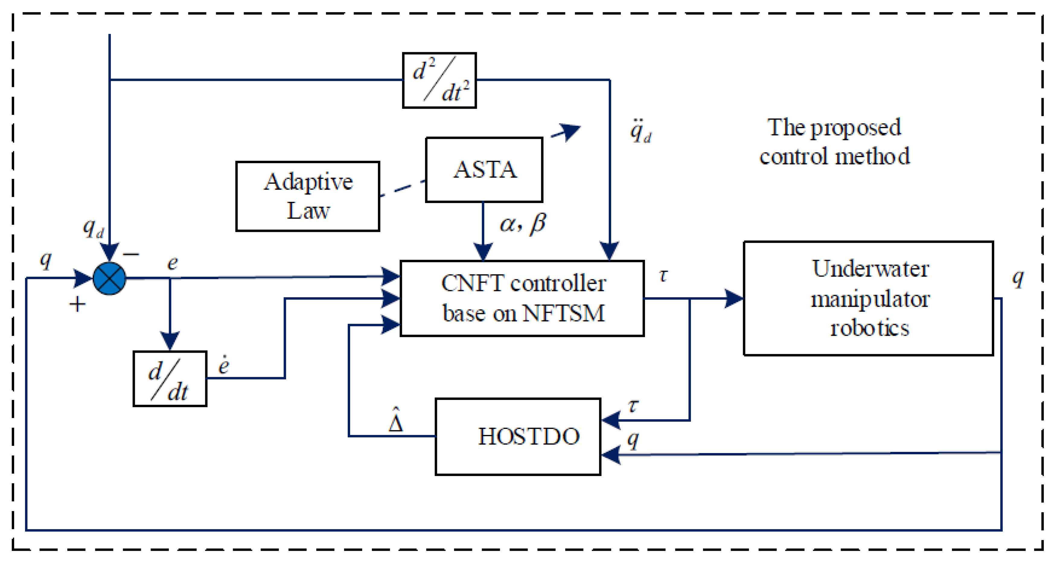
The block diagram of our newly proposed control method is given in Figure 1.

It can be observed that the proposed CNFT control scheme (8) contains no discontinuous terms compared with traditional SMC that uses the discontinuous function $sgn\left(s\right)$ thanks to the utilization of ASTA. Hence, the chattering issue can be successfully avoided. However, prior information of the lumped disturbances is not always accessible in real systems. To overcome this control limitation, the adaptation method is applied to approximate the designed parameters of the STA reaching control law, so that the prior information of the upper bound is not needed. On the other hand, NFTSM surface is designed in the proposed controller, thus the high control accuracy and fast convergence speed can be achieved and the singularity problem can be eliminated at the same time. The stability of the proposed control scheme is presented in Theorem 1.

Theorem 1.

For the underwater robot manipulator system (2), if an HOSTDO (4) and (5), NFTSM manifold (6), and control input (8) are proposed, the designed parameters for the ASTA are selected to satisfy (10) and (11), then the system position signal q will reach the given desired position signal $q_d$ in finite time, and it can be ensured that there is no occurrence of singularity and chattering problem during the whole tracking process.

Proof. 

Several similar control methods have been briefly proven in some other studies [37].

Substituting the CNFT control law (8) into (7), we have:

$$\begin{array}{c}\hfill \dot{s}={\sigma }_2\frac{l}{p}{\left|\dot{e}\right|}^{l/p-1}(-\alpha \frac{s}{{∥s∥}^{1/2}}-k_{1}s-\beta {\int }_0^t\frac{s}{∥s∥}dt-k_2{\int }_0^{t}sdt+\tilde{\Delta }(x_1,x_2,t))\end{array}.$$

(12)

We define the time–varying gain matrix P as follows:

$$P={\sigma }_2\frac{l}{p}{\left|\dot{e}\right|}^{l/p-1}.$$

(13)

Assumption 3.

The time–varying gain matrix is symmetric and positive definite. The largest and smallest eigenvalues of the time–varying gain matrix P are assumed to be bounded by upper (${\lambda }_M$) and lower (${\lambda }_m$) bound values respectively.

Assumption 4.

The estimation error of the lumped disturbances also satisfies the following inequality such that $∥D∥\le \delta ∥s∥$, where $D=\tilde{\Delta }(x_1,x_2,t)$, $\delta >0$ is a positive known constant, and $\tilde{\Delta }(x_1,x_2,t)=\Delta (x_1,x_2,t)-\widehat{\Delta }(x_1,x_2,t)$ is the bounded observer estimate error vector.

Considering (13) and Assumption 4, then (12) can be rewritten as:

$$\begin{array}{cc}\hfill \dot{s}& =-\alpha P\frac{s}{{∥s∥}^{1/2}}-k_{1}Ps+Pv+PD\hfill \\ \hfill \dot{v}& =-\beta \frac{s}{∥s∥}-k_{2}s\hfill \end{array}$$

(14)

where $v=-\beta {\int }_0^t\frac{s}{∥s∥}dt-k_2{\int }_0^{t}sdt$.

Remark 4.

It should be noted that in the NFTSM control method, the time–varying gain matrix P cannot be eliminated during the design process compared with the nominal STA–based sliding mode control [38], which makes the demonstration more difficult.

Then, select the Lyapunov function candidate as:

$$V=V_1(s,v)+\frac{1}{2{\mu }_1}{(\alpha -{\alpha }^{*})}^2+\frac{1}{2{\mu }_2}{(\beta -{\beta }^{*})}^2$$

(15)

where ${\alpha }^{*},{\beta }^{*}$ are the upper bounds of $\alpha ,\beta$, respectively and ${\mu }_1,{\mu }_2>0$ are positive constants. The function $V_1(s,v)$ is given as:

$$\begin{array}{cc}\hfill & V_1(s,v)=(2\beta +\frac{{\alpha }^2}{2}{\lambda }_M)∥s∥+(k_2+\frac{k_1^2}{2}{\lambda }_M)s^{T}s\hfill \\ \hfill & +v^{T}Pv+\alpha k_1{\lambda }_M\frac{s^{T}s}{{∥s∥}^{1/2}}-k_1{s}^{T}Pv-\alpha \frac{v^{T}Ps}{{∥s∥}^{1/2}}.\hfill \end{array}$$

(16)

It can be demonstrated that $V_1(s,v)$ is positive definite since:

$$V_1\ge 2\beta ∥s∥+k_2{s}^{T}s+\frac{1}{2}{v}^{T}Pv+\frac{1}{2}{\chi }^{T}P\chi$$

(17)

where $\chi =\alpha \frac{s}{{∥s∥}^{1/2}}+k_{1}s-v$.

The time derivative of Lyapunov function (16) can be expressed as:

$$\begin{array}{cc}\hfill {\dot{V}}_1& =(2\beta +\frac{{\alpha }^2}{2}{\lambda }_M)\frac{s^T\dot{s}}{∥s∥}+(2k_2+k_1^2{\lambda }_M)s^T\dot{s}+2v^{T}P\dot{v}+\frac{3}{2}\alpha k_1{\lambda }_M\frac{s^T\dot{s}}{{∥s∥}^{1/2}}\hfill \\ & -k_1(v^{T}P\dot{s}+s^{T}P\dot{v})-\alpha \frac{v^{T}P\dot{s}}{{∥s∥}^{1/2}}+\frac{\alpha }{2}\frac{\left(v^{T}Ps\right)\left(s^T\dot{s}\right)}{{∥s∥}^{5/2}}-\alpha \frac{s^{T}P\dot{v}}{{∥s∥}^{1/2}}.\hfill \end{array}$$

Lemma 2 ([37]).

As we have the diagonal matrix $P=P^T\ge 0$, the following inequality holds:

$$\frac{\left(v^{T}Ps\right)\left(v^{T}Ps\right)}{{∥s∥}^{5/2}}\le \frac{v^T{P}^{2}v}{{∥s∥}^{1/2}}.$$

(18)

Substituting (14) and considering the inequality in Lemma 2, the equation becomes:

$$\begin{array}{cc}\hfill {\dot{V}}_1& \le -\frac{\alpha }{{∥s∥}^{1/2}}{\lambda }_m(\beta +{\lambda }_M\frac{{\alpha }^2}{2})∥s∥-{\lambda }_m(k_1\beta +2{\lambda }_M{\alpha }^2{k}_1)∥s∥+\frac{2{\alpha }^2}{{∥s∥}^{1/2}}{\lambda }_M^2∥v∥{∥s∥}^{1/2}\hfill \\ & -\frac{{\lambda }_m}{{∥s∥}^{1/2}}(\frac{5}{2}\alpha k_1^2{\lambda }_M+\alpha k_2){∥s∥}^2-{\lambda }_m(k_1{k}_2+k_1^3{\lambda }_M){∥s∥}^2+2k_1^2{\lambda }_M^2∥s∥∥v∥\hfill \\ & +\frac{4\alpha k_1{\lambda }_M^2}{{∥s∥}^{1/2}}∥s∥∥v∥-k_1{\lambda }_m^2{∥v∥}^2-\frac{\alpha }{2}{\lambda }_m^2\frac{{∥v∥}^2}{{∥s∥}^{1/2}}+{\lambda }_M(2\beta +\frac{{\alpha }^2}{2}{\lambda }_M)\delta ∥s∥\hfill \\ & +{\lambda }_M(k_1^2{\lambda }_M+2k_2)\delta {∥s∥}^2+\frac{3}{2}\alpha k_1{\lambda }_M^2\frac{\delta {∥s∥}^2}{{∥s∥}^{1/2}}+k_1{\lambda }_M^2\delta ∥v∥∥s∥+\frac{3}{2}\alpha {\lambda }_M^2\delta ∥v∥{∥s∥}^{1/2}.\hfill \end{array}$$

Define a new vector $\zeta ={\left[\begin{array}{ccc}{∥s∥}^{1/2}& ∥s∥& ∥v∥\end{array}\right]}^T$, thus it can be obtained that when $\zeta$ converges to zero, s and v will also converge to zero at the same time.

Re–express the last inequality as:

$${\dot{V}}_1\le -\frac{1}{{∥s∥}^{1/2}}{\zeta }^T\Omega \zeta -{\zeta }^T\Psi \zeta$$

(19)

where $\Omega =\left[\begin{array}{ccc}{\Omega }_{11}& 0& {\Omega }_{13}\\ 0& {\Omega }_{22}& {\Omega }_{23}\\ {\Omega }_{13}& {\Omega }_{23}& {\Omega }_{33}\end{array}\right]$, $\Psi =\left[\begin{array}{ccc}{\psi }_{11}& 0& {\psi }_{13}\\ 0& {\psi }_{22}& {\psi }_{23}\\ {\psi }_{13}& {\psi }_{23}& {\psi }_{33}\end{array}\right]$, with elements:

${\Omega }_{11}={\lambda }_m(\alpha \beta +\frac{{\alpha }^3}{2}{\lambda }_M)$, ${\Omega }_{13}=-{\alpha }^2{\lambda }_M^2$, ${\Omega }_{22}={\lambda }_m(\alpha k_2+\frac{5}{2}\alpha k_1^2{\lambda }_M)-\frac{3}{2}\alpha k_1{\lambda }_M^2\delta$,

${\Omega }_{23}=-2\alpha k_1{\lambda }_M^2$, ${\Omega }_{33}=\frac{\alpha }{2}{\lambda }_m^2$,

and

${\psi }_{11}={\lambda }_m(k_1\beta +2{\alpha }^2{k}_1{\lambda }_M)-{\lambda }_M(2\beta +\frac{{\alpha }^2}{2}{\lambda }_M)\delta$, ${\psi }_{13}=-\frac{3}{4}\alpha {\lambda }_M^2\delta$,

${\psi }_{22}={\lambda }_m(k_1{k}_2+k_1^2{\lambda }_M)-{\lambda }_M(k_1^2{\lambda }_M+2k_2)\delta$, ${\psi }_{23}=-k_1^2{\lambda }_M^2-\frac{k_1}{2}{\lambda }_M^2\delta$, ${\psi }_{33}=k_1{\lambda }_m^2$.

The function ${\dot{V}}_1$ will be negative definite if the matrices $\Omega ={\Omega }^T>0$, $\Psi ={\Psi }^T>0$. By selecting the parameters, it can be ensured that the diagonal elements and the determinants are positive. Therefore, the parameters should satisfy the following inequalities to ensure $\Omega ={\Omega }^T>0$ if:

$$\begin{array}{c}\hfill \alpha >0,\beta >4{\alpha }^2\frac{{\lambda }_M^4}{{\lambda }_m^3},k_1>\frac{3}{5}\frac{{\lambda }_M}{{\lambda }_m}\delta ,k_2>16k_1^2\frac{{\lambda }_M^4}{{\lambda }_m^3},\end{array}$$

(20)

and $\Psi ={\Psi }^T>0$ if:

$$\begin{array}{cc}\hfill & \alpha >0,\beta >0,k_1>max\left\{2\frac{{\lambda }_M}{{\lambda }_m}\delta ,\delta \sqrt{\frac{9}{14}\frac{{\lambda }_M^3}{{\lambda }_m^3}}\right\},\hfill \\ \hfill & k_2>\frac{3k_1^2{\lambda }_M^4\delta +\frac{1}{2}{k}_1{\lambda }_M^4{\delta }^2{+k}_1^3{\lambda }_M(2{\lambda }_M^3-{\lambda }_m^3)}{{\lambda }_m^2(k_1{\lambda }_m-2{\lambda }_M\delta )}.\hfill \end{array}$$

(21)

Hence, the obtained matrices $\Omega$, $\Psi$ are symmetric positive definite when the given conditions (20) and (21) hold. Then we have:

$${\dot{V}}_1\le -\frac{{\lambda }_{min}(\Omega )}{{∥s∥}^{1/2}}{∥\zeta ∥}^2-{\lambda }_{min}(\Psi ){∥\zeta ∥}^2$$

(22)

where ${\lambda }_{min}(\Omega )$ and ${\lambda }_{min}(\Psi )$ are the smallest eigenvalues of the matrices $\Omega$ and $\Psi$, respectively. Thus, the candidate Lyapunov function in (16) can be rewritten as $V_1(s,v)={\overline{\zeta }}^{T}Q\overline{\zeta }$, where $\overline{\zeta }={\left[\begin{array}{ccc}\frac{s^T}{{∥s∥}^{1/2}}& s^T& v^T\end{array}\right]}^T$, and $Q=Q^T>0$, given as:

$$Q=\left[\begin{array}{ccc}2\beta +\frac{{\alpha }^2}{2}{\lambda }_M& \frac{\alpha }{2}{k}_1{\lambda }_M& -\frac{\alpha P}{2}\\ \frac{\alpha }{2}{k}_1{\lambda }_M& k_2+\frac{k_1^2}{2}{\lambda }_M& -\frac{k_{1}P}{2}\\ -\frac{\alpha P}{2}& -\frac{k_{1}P}{2}& P\end{array}\right]$$

then the following inequality holds:

$${\lambda }_{min}\left(Q\right){∥\overline{\zeta }∥}^2\le V_1\le {\lambda }_{max}\left(Q\right){∥\overline{\zeta }∥}^2$$

(23)

where $∥\overline{\zeta }∥=∥\zeta ∥$, and ${\lambda }_{min}\left(Q\right),{\lambda }_{max}\left(Q\right)>0$ are the lowest and highest eigenvalues of the matrix Q, respectively.

Besides, consider the following fact:

$${∥s∥}^{1/2}\le ∥\zeta ∥\le \frac{{V_1}^{1/2}}{\sqrt{{\lambda }_{min}\left(Q\right)}}.$$

(24)

Then we have:

$${\dot{V}}_1\le -{\rho }_1{V_1}^{1/2}-{\rho }_2{V}_1\le -{\rho }_1{V_1}^{1/2}$$

(25)

where ${\rho }_1=\frac{\sqrt{{\lambda }_{min}\left(Q\right)}{\lambda }_{min}(\Omega )}{{\lambda }_{max}\left(Q\right)}$, ${\rho }_2=\frac{{\lambda }_{min}(\Psi )}{{\lambda }_{max}\left(Q\right)}$.

Since ${\alpha }^{*},{\beta }^{*}$ are the upper bounds of $\alpha ,\beta$, it can be obtained that $\tilde{\alpha }=\alpha -{\alpha }^{*}<0$, $\tilde{\beta }=\beta -{\beta }^{*}<0$. Then the time derivative of the Lyapunov function candidate (15) can be given as:

$$\begin{array}{cc}\hfill \dot{V}& ={\dot{V}}_1+\frac{1}{{\mu }_1}\tilde{\alpha }\dot{\alpha }+\frac{1}{{\mu }_2}\tilde{\beta }\dot{\beta }\hfill \\ \hfill & \le -{\rho }_1{V_1}^{1/2}-\frac{{\omega }_1}{\sqrt{2{\mu }_1}}\left|\tilde{\alpha }\right|-\frac{{\omega }_2}{\sqrt{2{\mu }_2}}\left|\tilde{\beta }\right|+\frac{1}{{\mu }_1}\tilde{\alpha }\dot{\alpha }+\frac{1}{{\mu }_2}\tilde{\beta }\dot{\beta }+\frac{{\omega }_1}{\sqrt{2{\mu }_1}}\left|\tilde{\alpha }\right|+\frac{{\omega }_2}{\sqrt{2{\mu }_2}}\left|\tilde{\beta }\right|.\hfill \end{array}$$

(26)

It should be noted that the following inequality holds:

$${(x^2+y^2+z^2)}^{1/2}\le \left|x\right|+\left|y\right|+\left|z\right|.$$

(27)

Thus this leads to:

$$\dot{V}\le -{\rho }_3{V}^{1/2}+\frac{1}{{\mu }_1}\tilde{\alpha }\dot{\alpha }+\frac{1}{{\mu }_2}\tilde{\beta }\dot{\beta }+\frac{{\omega }_1}{\sqrt{2{\mu }_1}}\left|\tilde{\alpha }\right|+\frac{{\omega }_2}{\sqrt{2{\mu }_2}}\left|\tilde{\beta }\right|,$$

(28)

where ${\rho }_3=min\left\{{\rho }_1,{\omega }_1,{\omega }_2\right\}$. Then it can be written as:

$$\dot{V}\le -{\rho }_3{V}^{1/2}+\Theta ,$$

(29)

where $\Theta =-\left|\tilde{\alpha }\right|\left(\frac{\dot{\alpha }}{{\mu }_1}-\frac{{\omega }_1}{\sqrt{2{\mu }_1}}\right)-\left|\tilde{\beta }\right|\left(\frac{\dot{\beta }}{{\mu }_2}-\frac{{\omega }_2}{\sqrt{2{\mu }_2}}\right)$.

Supposing that $\alpha >{\alpha }_m$ and $\left|s_i\right|\ge {\rho }_0$, and we choose ${\Phi }_1={\mu }_1$, ${\Phi }_2={\mu }_2$, then we have:

$$\dot{\alpha }={\omega }_1\sqrt{\frac{{\Phi }_1}{2}},\dot{\beta }=2k\dot{\alpha }={\omega }_2\sqrt{\frac{{\Phi }_2}{2}},$$

$$\Theta =-\left|\tilde{\alpha }\right|\left(\frac{\dot{\alpha }}{{\mu }_1}-\frac{{\omega }_1}{\sqrt{2{\mu }_1}}\right)-\left|\tilde{\beta }\right|\left(\frac{\dot{\beta }}{{\mu }_2}-\frac{{\omega }_2}{\sqrt{2{\mu }_2}}\right).$$

If we define $\kappa =\frac{{\omega }_2}{2{\omega }_1}\sqrt{\frac{{\Phi }_2}{{\Phi }_1}}>0$, we can obtain $\Theta =0$,

$$\dot{V}\le -{\rho }_3{V}^{1/2}.$$

(30)

It should also be noted that the finite–time convergence can be ensured when the adaptive gains satisfy the inequalities (20) and (21). Thus the positive definiteness of the matrices $\Omega$, $\Psi$ and the convergence of whole processing system can be guaranteed.

Supposing $\alpha >{\alpha }_m$ and $\left|s_i\right|<{\rho }_0$, the adaptive gains can be given as:

$$\dot{\alpha }=-{\omega }_1\sqrt{\frac{{\Phi }_1}{2}},\dot{\beta }=-{\omega }_2\sqrt{\frac{{\Phi }_2}{2}},$$

and we have:

$$\Theta =2\left|\alpha -{\alpha }^{*}\right|\frac{{\omega }_1}{\sqrt{2{\mu }_1}}+2\left|\beta -{\beta }^{*}\right|\frac{{\omega }_2}{\sqrt{2{\mu }_2}}.$$

Since $\alpha ,\beta$ are bounded by ${\alpha }^{*},{\beta }^{*}$, and ${\omega }_1,{\omega }_2,{\mu }_1,{\mu }_2$ are chosen to be positive constants, then we have $\Theta >0$. According to [39], V is bounded which means all the signals have bounds. Therefore, the tracking errors can converge to a small neighborhood of the origin.

When $\alpha \le {\alpha }_m$, the adaptive gains are:

$$\dot{\alpha }=r_0,\dot{\beta }=2\kappa r_0,\alpha ={\alpha }_0+r_{0}t,\beta ={\beta }_0+2\kappa r_{0}t,$$

where ${\alpha }_0,{\beta }_0$ are the initial value of $\alpha$ and $\beta$, which are assumed to be 0 for simplicity.

Then we have the parameter $\Theta$ given as:

$$\begin{array}{cc}\hfill \Theta & =-\left|\tilde{\alpha }\right|(\frac{r_0}{{\mu }_1}-\frac{{\omega }_1}{\sqrt{2{\mu }_1}})-\left|\tilde{\beta }\right|(\frac{2\kappa r_0}{{\mu }_2}-\frac{{\omega }_2}{\sqrt{2{\mu }_2}})\hfill \\ \hfill & =-\left|r_{0}t-{\alpha }^{*}\right|(\frac{r_0}{{\mu }_1}-\frac{{\omega }_1}{\sqrt{2{\mu }_1}})-\left|2\kappa r_{0}t-{\beta }^{*}\right|(\frac{2\kappa r_0}{{\mu }_2}-\frac{{\omega }_2}{\sqrt{2{\mu }_2}}).\hfill \end{array}$$

It can be observed that when $\alpha \le {\alpha }_m$, $\Theta$ in (29) is negative. Hence, $\dot{V}$ would be sign indefinite [40]. However, $\alpha$ will increase with time in this case. As soon as $\alpha$ increases over the small constant ${\alpha }_m$, then (29) is valid and V starts decreasing. In order to accelerate the deceleration process, one can choose a larger $r_0$.

In conclusion, when $\left|s_i\right|>{\rho }_0$ which means the sliding parameter $s_i$ is far away from the sliding mode surface, it can reach the domain $\left|s_i\right|\le {\rho }_0$ within limited time. During the adaptation process, $s_i$ may leave the domain in finite time due to the increase of $\alpha$. However, it can always remain in a larger domain $\left|s_i\right|\le {\overline{\rho }}_0$, ${\overline{\rho }}_0>{\rho }_0$. Thus, the whole control system can remain stable and bounded in finite time according to Lemma 1. Therefore, the proof of Theorem 1 is completed.  □

4. Simulation Results

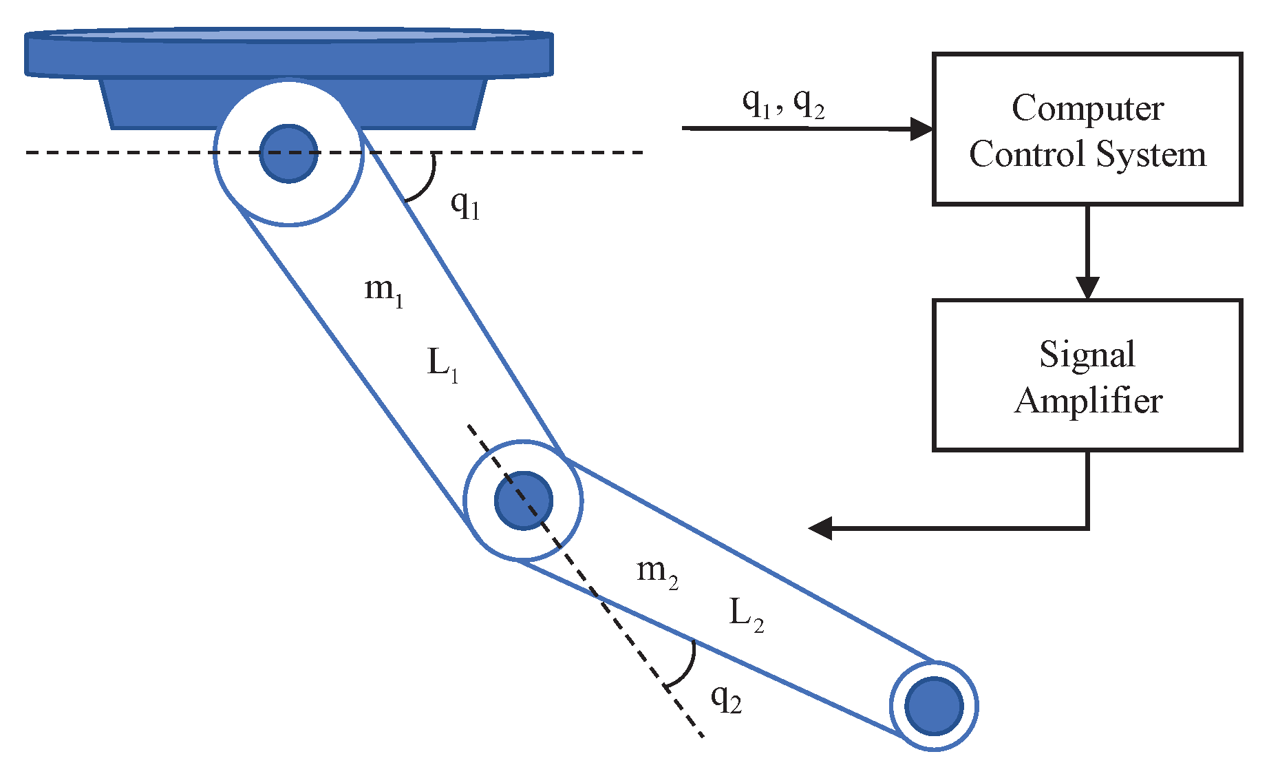
To demonstrate the effectiveness and advantage of our newly proposed control method, the simulations on a 2–DOF underwater robot manipulator, which is shown in Figure 2, are performed in this section. The rigid body dynamics of the manipulator system are taken from [31], and the underwater force ${\tau }_w(q,\dot{q})$ is taken from [32], thus the dynamics of the 2–DOF underwater robot manipulator in the form of (1) is given as:

$$M\left(q\right)\ddot{q}+C(q,\dot{q})\dot{q}+G\left(q\right)+{\tau }_w(q,\dot{q})={\tau }_{edis}+\tau$$

(31)

with matrices:

$$\begin{array}{cc}\hfill M\left(q\right)& =\left[\begin{array}{cc}(m_1+m_2{)L}_1^2+m_2{L}_2^2+2m_2{L}_1{L}_2{c}_2& m_2{L}_2^2+m_2{L}_1{L}_2{c}_2\\ m_2{L}_2^2+m_2{L}_1{L}_2{c}_2& m_2{L}_2^2\end{array}\right],\hfill \\ \hfill C(q,\dot{q})& =\left[\begin{array}{cc}-m_2{L}_1{L}_2{s}_2{\dot{q}}_2& -m_2{L}_1{L}_2{s}_2({\dot{q}}_1+{\dot{q}}_2)\\ m_2{L}_1{L}_2{s}_2{\dot{q}}_1& 0\end{array}\right],\hfill \\ \hfill G\left(q\right)& =\left[\begin{array}{c}(m_1+m_2)L_{1}g{c}_2+m_2{L}_{2}g{c_1}_2\\ m_2{L}_{2}g{c_1}_2\end{array}\right],\hfill \\ \hfill {\tau }_B& =\left[\begin{array}{c}{\tau }_{B1}\\ {\tau }_{B2}\end{array}\right],{\tau }_D=\left[\begin{array}{c}{\tau }_{D1}\\ {\tau }_{D2}\end{array}\right]\hfill \end{array}$$

in which $s_2=sin\left(q_2\right)$, $c_2=cos\left(q_2\right)$, $c_{12}=cos(q_1+q_2)$; $m_1$, $m_2$ are the masses; $L_1$, $L_2$ are the lengths; and g is the gravity acceleration. The hydrodynamic forces ${\tau }_B$ and ${\tau }_D$ are given in Appendix A. In order to easily compare the performances of the proposed controller, traditional SM, NSM, and NFTSM control, which are referred to as controller 1, controller 2, and controller 3 respectively, are given in Appendix B. The parameters for the manipulator system and the model simulation are shown in

Table 1. Parameters of the manipulator system and the model simulation. Sliding mode (SM); adaptive super twisting algorithm (ASTA); higher–order super–twisting disturbance observer (HOSTDO).

Parameter	Value	Parameter	Value	Parameter	Value
Parameters of the manipulator system
$m_1$	3.39 kg	$D_1$	0.04 m	$L_1$	1 m
$m_2$	3.39 kg	$D_2$	0.04 m	$L_2$	1 m
${\rho }_f$	1000 kg/m${}^3$	$C_D$	0.6	g	9.8 m/s${}^2$
${\rho }_m$	2700 kg/m${}^3$
Parameters of the model simulation comparison
Parameters of SM surfaces		${\sigma }_0$	1	${\sigma }_0^{\prime }$	1
		${\sigma }_1$	1	${\sigma }_2$	1
		l	7	$l^{\prime }$	7
		p	9	$p^{\prime }$	9
		$\phi$	1.3
Gains of SM reaching laws		$k_0$	20	$k_1^{\prime }$	20
		$k_1^{″}$	20	${\eta }_0$	0.1
		${\eta }_0^{\prime }$	0.1	${\eta }_0^{″}$	0.1
		${\gamma }_0$	2	${\gamma }_0^{\prime }$	2
		${\gamma }_0^{″}$	2	${\eta }_0$	0.1
Parameters of the ASTA		$k_1$	15	$k_2$	0.1
		${\omega }_1$	5	${\Phi }_1$	2
		${\alpha }_m$	0.5	$r_0$	0.5
		${\rho }_0$	0.05	$\kappa$	0.5
Parameters of the HOSTDO		${\xi }_1$	8	${\xi }_2$	22
		${\xi }_3$	8	${\xi }_4$	2

.

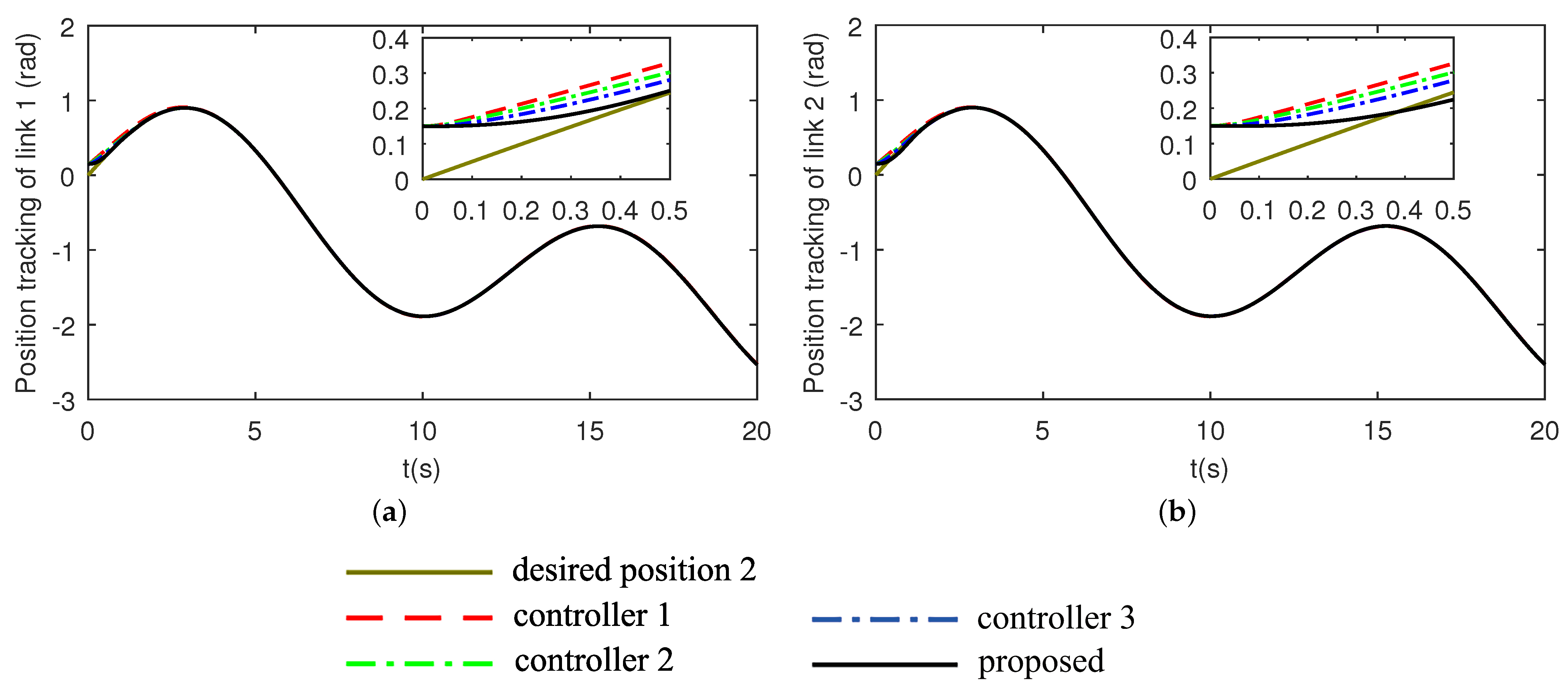
The referred trajectory for both links is given as $q_d={\left[\begin{array}{cc}{q}_{d1}& q_{d2}\end{array}\right]}^T$, $q_{d1}=q_{d2}=sin\left(0.5t\right)+cos\left(0.15t\right)-1$. The time–varying lumped disturbances for the 2–DOF underwater robot manipulator are designed as ${\tau }_{edis}={\left[{\tau }_{edis1}{\tau }_{edis2}\right]}^T$ with ${\tau }_{edis1}={\tau }_{edis2}=0.5+1.5sin\left(t\right)$. Simulations are performed to compare the differences of the controllers in terms of the position precision, response speed, and the chattering phenomenon. The obtained simulation results are given in Figure 3, Figure 4, Figure 5, Figure 6 and Figure 7.

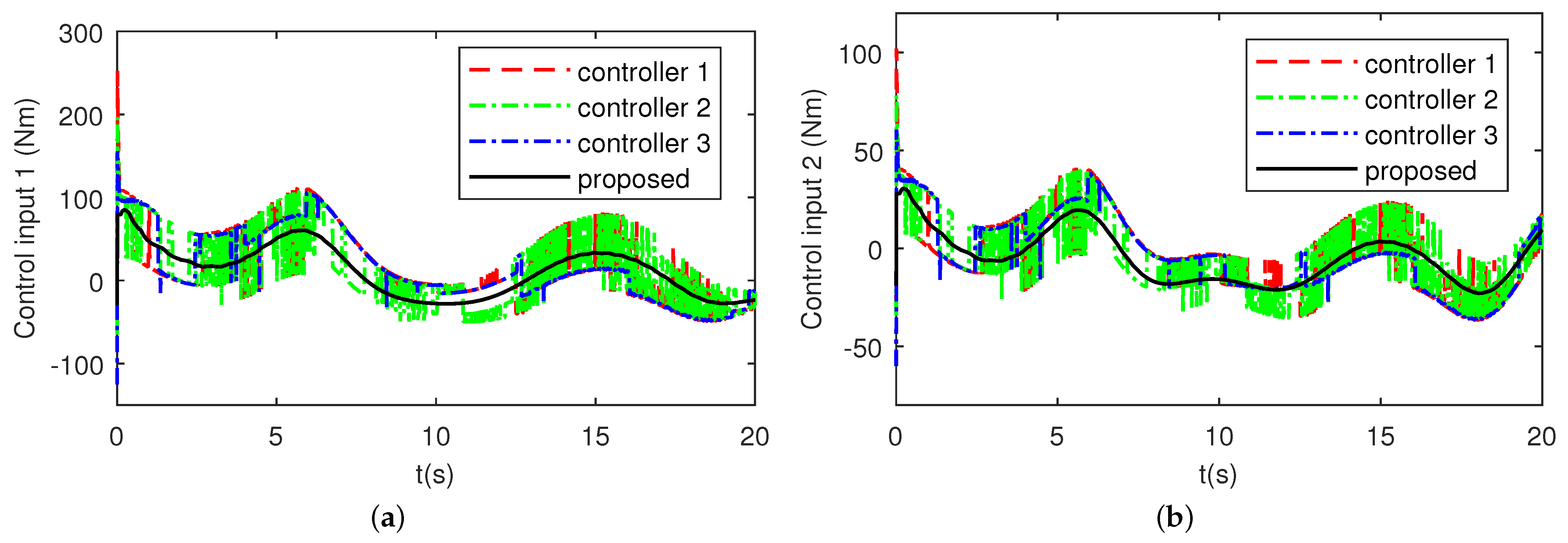
Figure 3 shows the trajectory tracking performances of four controllers for the 2–DOF underwater robot manipulator under the lumped disturbances. It can be seen that good tracking performance can be ensured by all four controllers, while the proposed control method approaches the desired trajectories with the highest reaching speed. Thanks to the utilization of ASTA, no noticeable chattering problem occurs in our proposed controller as shown in Figure 4. The performances in three comparing controllers encounter with the instantaneous jump in the control torques. However, the joint servo–motors can not reverse their rotation direction immediately which may cause failure or severe damage. In comparison, the proposed controller generates a smooth control input, thus the strongest robustness of our proposed controller is demonstrated.

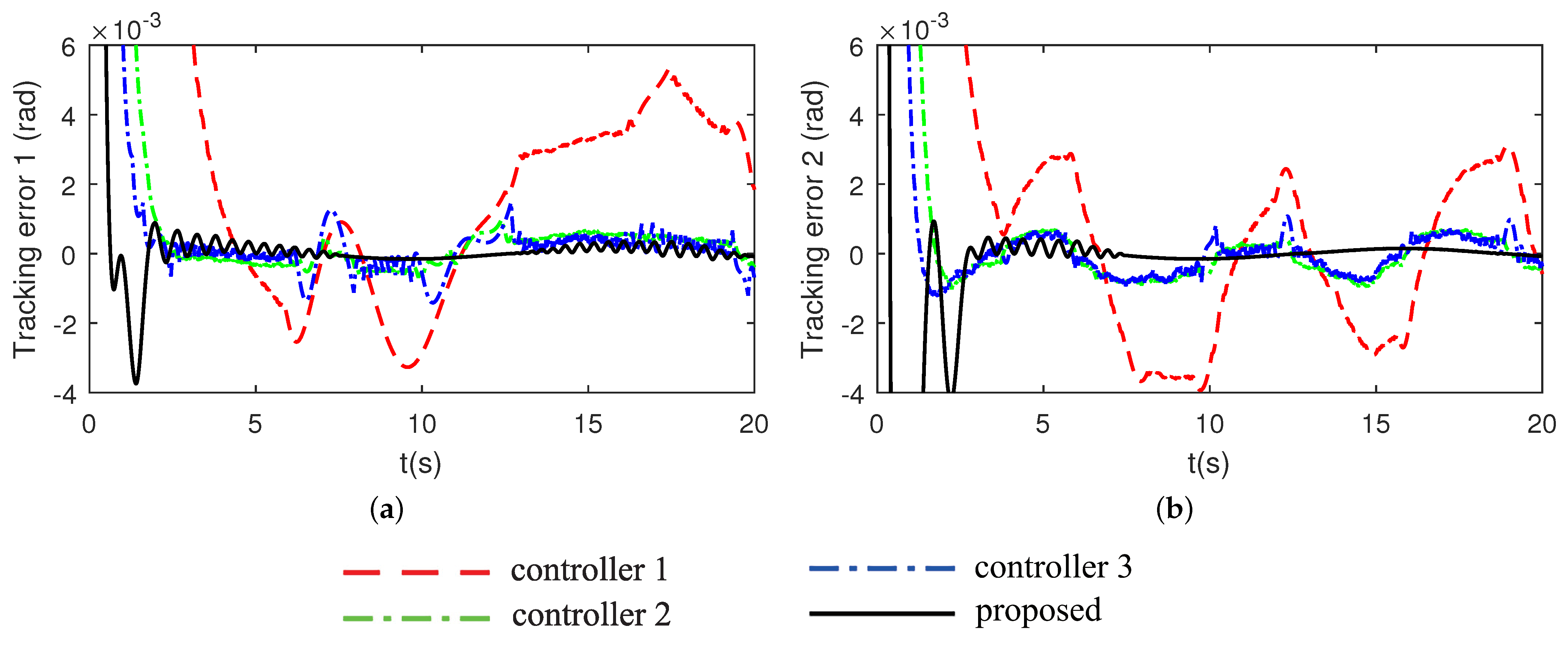
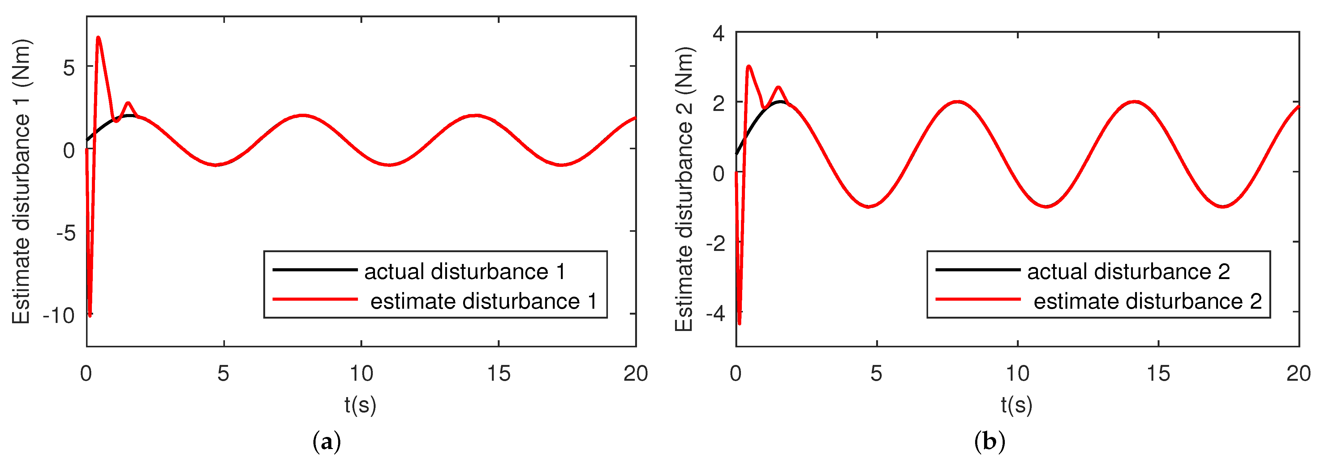
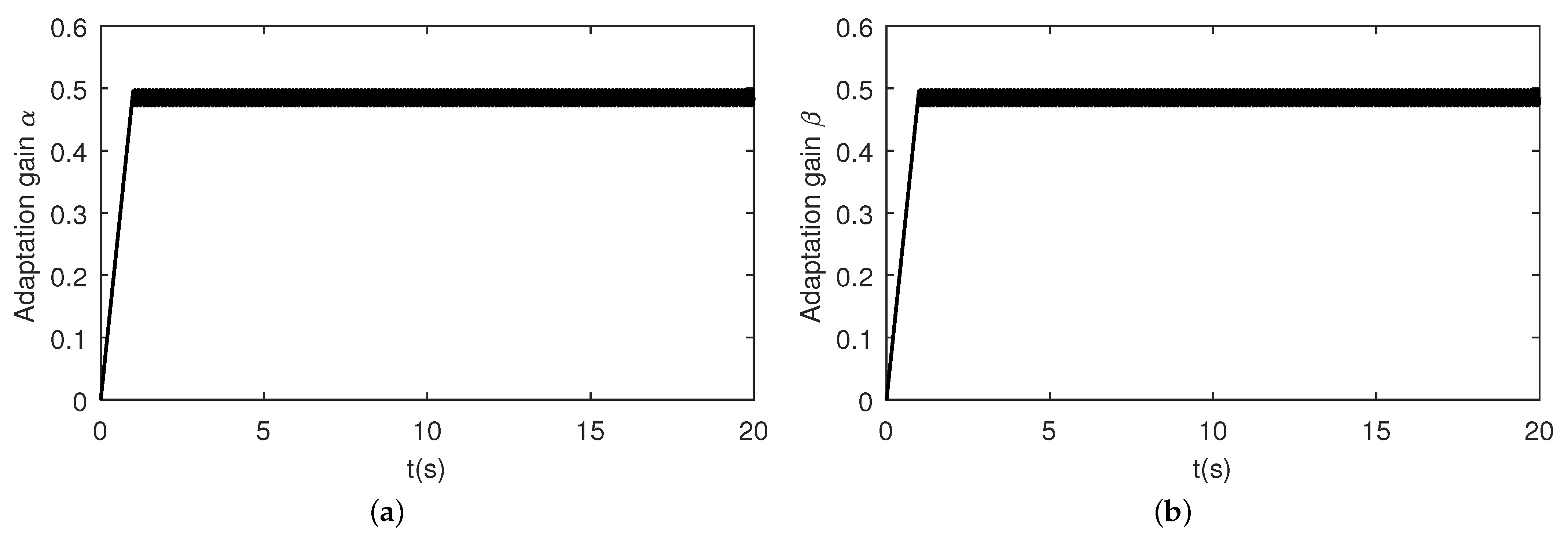
Furthermore, in Figure 5, the fastest convergence and highest precision are obtained by our proposed controller. It can be seen that controller 1 shows the worst tracking precision when reaching the steady state. The steady tracking errors of controller 2 and 3 oscillate near the origin with a relatively higher amplitude than the proposed control. The estimations of the lumped disturbances are given in Figure 6, which nearly overlap the given disturbance signal. The compensation capability of the HOSTDO should be valued in the real applications since the actual currents and waves are impossible to calculate and proper estimations can significantly improve the disturbance–attenuation ability. The adaptation gains of the ASTA are shown in Figure 7, which release the limitation of the need for upper bound prior information of the lumped disturbances.

To further analyze the position tracking errors and energy consumption of the four controllers, the following integrated absolute error (IAE) [41], root mean square error (RMSE) [27], and energy of control input (ECI) [42] are taken into consideration, which are defined as:

$$\begin{array}{c}\hfill {IAE}_i=\sum _{k=1}^N\left|e_i\left(k\right)\right|;{RMSE}_i=\sqrt{\frac{1}{N}\sum _{k=1}^N{e}_i^2\left(k\right)};{ECI}_i=\sum _{k=1}^N\left|{\tau }_i^2\left(k\right)\right|\end{array}$$

(32)

where i is the link number; N is the number of samples; and $e_i\left(k\right)$, ${\tau }_i\left(k\right)$ are the trajectory tracking error and control input of link i at the $k^{th}$ sampling instant, respectively.

IAE and RMSE are used to evaluate the tracking performance while ECI is adopted to evaluate the control input energy consumption. Thus, the control target is to have a lower IAE, RMSE, and ECI so that better performances can be obtained with less energy consumption. The comparison results of the four controllers are shown in

Table 2. Tracking performance comparisons.

Type of Controller	Link	IAE	RMSE	ECI
Controller 1	1	18.120	0.022718	4.1162 $\times {10}^6$
	2	15.813	0.021560	7.4115 $\times {10}^5$
Controller 2	1	7.7463	0.016877	4.5057 $\times {10}^6$
	2	7.7831	0.016592	8.1977 $\times {10}^5$
Controller 3	1	5.7875	0.014082	4.2817 $\times {10}^6$
	2	5.5934	0.013763	7.5878 $\times {10}^5$
Proposed	1	3.4521	0.011636	2.0673 $\times {10}^6$
	2	5.2355	0.012449	3.9025 $\times {10}^5$

.

It should be noted that the ECI varies significantly due to the existence of the lumped disturbances. The ECI values of our proposed control method are only 50.2% and 52.7% for Controller 1, 45.9% and 47.6% for Controller 2, and 48.3% and 51.4% for Controller 3, respectively, which indicate that our proposed control consumes less input energy in the presence of the lumped disturbances. Furthermore, our proposed control still guarantees the best tracking precision in this case when considering the values of IAE and RMSE. Thus, considering the unknown lumped disturbances, our proposed control method can obtain the best tracking precision with the least control input energy consumption among the four controllers.

5. Conclusions

In this paper, a novel HOSTDO–based CNFT control with the ASTA method was proposed for underwater robot manipulators under time–varying lumped disturbances. The proposed controller utilized the NFTSM manifold and the ASTA method in the CNFT control scheme to ensure high control precision, singularity–free, chattering–free, and fast convergence. Meanwhile, the HOSTDO was used in this paper to estimate and compensate the lumped disturbances, which strengthen the robustness of our newly proposed controller. It should also be noted that the adaptation method was presented in the ASTA scheme so that prior information of the upper bound of the lumped disturbances was not needed. The stability of closed–loop system was demonstrated by the Lyapunov theory considering the ASTA dynamics and NFTSM surface. Finally, the effectiveness and robustness of our newly proposed control method were verified by comparing with the other three controllers on a 2–DOF underwater manipulator system. Although the proposed control is based on the underwater manipulators, it can also be utilized in some other robot system such as the manipulators on land, autonomous underwater vehicles, and so on.

In the proposed control method, the uncertain system modeling and the unknown external disturbances in the underwater manipulator system have been considered. However, it is still not clear how the robot interacts within underwater circumstances. In the future, we will intend to conduct underwater experiments to investigate the specific values of hydrodynamic coefficients, which will help us to build a more accurate mathematical dynamic model. To improve the application ability, the effects of time delays and actuator faults will be studied.

References

- Qiao, L.; Zhang, W. Double–loop integral terminal sliding mode tracking control for UUVs with adaptive dynamic compensation of uncertainties and disturbances. IEEE J. Ocean. Eng. 2019, 44, 29–53. [Google Scholar] [CrossRef]
- Leabourne, K.N.; Rock, S.M. Model development of an underwater manipulator for coordinated arm–vehicle control. In Proceedings of the OCEANS’98, Nice, France, 28 September–1 October 1998; Volume 2, pp. 941–946. [Google Scholar]
- Ioi, K.; Itoh, K. Modelling and simulation of an underwater manipulator. Adv. Robot. 1989, 4, 303–317. [Google Scholar] [CrossRef]
- Zhang, M.; Liu, X.; Tian, Y. Modeling Analysis and Simulation of Viscous Hydrodynamic Model of Single–DOF Manipulator. J. Mar. Sci. Eng. 2019, 7, 261. [Google Scholar] [CrossRef] [Green Version]
- Wang, T.; You, Z.; Song, W.; Zhu, S. Dynamic Analysis of an Underwater Cable–Driven Manipulator with a Fluid–Power Buoyancy Regulation System. Micromachines 2020, 11, 1042. [Google Scholar] [CrossRef] [PubMed]
- Tang, J.; Zhang, Y.; Huang, F. Design and Kinematic Control of the Cable–Driven Hyper–Redundant Manipulator for Potential Underwater Applications. Appl. Sci. 2019, 9, 1142. [Google Scholar] [CrossRef] [Green Version]
- Yao, J.; Wang, C. Model reference adaptive control for a hydraulic underwater manipulator. J. Vib. Control 2012, 18, 893–902. [Google Scholar] [CrossRef]
- Barbalata, C.; Dunnigan, M.W.; Petillot, Y. Coupled and Decoupled Force/Motion Controllers for an Underwater Vehicle–Manipulator System. J. Mar. Sci. Eng. 2018, 6, 96. [Google Scholar] [CrossRef] [Green Version]
- Zhou, Z.; Tang, G.; Huang, H.; Han, L.; Xu, R. Adaptive nonsingular fast terminal sliding mode control for underwater manipulator robotics with asymmetric saturation actuators. Control Theory Technol. 2020, 18, 81–91. [Google Scholar] [CrossRef]
- Yang, C.; Yao, F.; Zhang, M.; Zhang, Z.; Wu, Z.; Dan, P. Adaptive Sliding Mode PID Control for Underwater Manipulator Based on Legendre Polynomial Function Approximation and Its Experimental Evaluation. Appl. Sci. 2020, 10, 1728. [Google Scholar] [CrossRef] [Green Version]
- Xu, R.; Tang, G.; Han, L.; Huang, H.; Xie, D. Robust finite–time attitude tracking control of a CMG–based AUV with unknown disturbances and input saturation. IEEE Access 2019, 7, 56409–56422. [Google Scholar] [CrossRef]
- Le, T.H.; Thanh, H.L.N.N.; Huynh, T.T.; Van, M.; Hoang, Q.D.; Do, T.D. Robust Position Control of an Over–actuated Underwater Vehicle under Model Uncertainties and Ocean Current Effects Using Dynamic Sliding Mode Surface and Optimal Allocation Control. Sensors 2021, 21, 747. [Google Scholar]
- Thanh, H.L.N.N.; Vu, M.T.; Mung, N.X.; Nguyen, N.P.; Phuong, N.T. Perturbation Observer–Based Robust Control Using a Multiple Sliding Surfaces for Nonlinear Systems with Influences of Matched and Unmatched Uncertainties. Mathematics 2020, 8, 1371. [Google Scholar] [CrossRef]
- Vu, M.T.; Thang, H.T.T.L.; Thang, Q.; Duc, T.; Hoang, Q.D.; Le, T.H. Station–Keeping Control of a Hovering Over–Actuated Autonomous Underwater Vehicle Under Ocean Current Effects and Model Uncertainties in Horizontal Plane. IEEE Access 2021, 9, 6855–6867. [Google Scholar] [CrossRef]
- Yang, L.; Yang, J. Nonsingular fast terminal sliding–mode control for nonlinear dynamical systems. Int. J. Robust Nonlinear Control 2011, 21, 1865–1879. [Google Scholar] [CrossRef]
- Zhao, L.; Jia, Y. Decentralized adaptive attitude synchronization control for spacecraft formation using nonsingular fast terminal sliding mode. Nonlinear Dyn. 2014, 78, 2779–2794. [Google Scholar] [CrossRef]
- Xu, S.S.; Chen, C.; Wu, Z. Study of nonsingular fast terminal sliding–mode fault–tolerant control. IEEE Trans. Ind. Electron. 2015, 62, 3906–3913. [Google Scholar] [CrossRef]
- Zhang, L.; Liu, L.; Wang, Z.; Xia, Y. Continuous finite–time control for uncertain robot manipulators with integral sliding mode. IET Control Theory Appl. 2018, 12, 1621–1627. [Google Scholar] [CrossRef]
- Van, M.; Kang, H.J.; Suh, Y.S. Second order sliding mode–based output feedback tracking control for uncertain robot manipulators. Int. J. Adv. Robot. Syst. 2013, 10, 16. [Google Scholar] [CrossRef] [Green Version]
- Levant, A.; Alelishvili, L. Integral high–order sliding modes. IEEE Trans. Autom. Control 2007, 52, 1278–1282. [Google Scholar] [CrossRef] [Green Version]
- Li, X.; Yu, X.; Han, Q. Stability analysis of second–order sliding mode control systems with input–delay using poincaré map. IEEE Trans. Autom. Control 2013, 58, 2410–2415. [Google Scholar] [CrossRef]
- Li, J.; Zhang, Q.; Yan, X.; Spurgeon, S.K. Integral sliding mode control for Markovian jump T–S fuzzy descriptor systems based on the super–twisting algorithm. IET Control Theory Appl. 2017, 11, 1134–1143. [Google Scholar] [CrossRef] [Green Version]
- Zhao, Z.; Gu, H.; Zhang, J.; Ding, G. Terminal sliding mode control based on super–twisting algorithm. J. Syst. Eng. Electron. 2017, 28, 145–150. [Google Scholar] [CrossRef]
- Rehman, F.U.; Mufti, M.R.; Din, S.U.; Afzal, H.; Qureshi, M.I.; Khan, D.M. Adaptive Smooth Super–Twisting Sliding Mode Control of Nonlinear Systems With Unmatched Uncertainty. IEEE Access 2020, 8, 177932–177940. [Google Scholar] [CrossRef]
- Shtessel, Y.; Taleb, M.; Plestan, F. A novel adaptive–gain supertwisting sliding mode controller: Methodology and application. Automatica 2012, 48, 759–769. [Google Scholar] [CrossRef]
- Van, M.; Ge, S.S.; Ren, H. Finite time fault tolerant control for robot manipulators using time delay estimation and continuous nonsingular fast terminal sliding mode control. IEEE T. Cybern. 2017, 47, 1681–1693. [Google Scholar] [CrossRef]
- Wang, Y.; Yan, F.; Ju, F.; Chen, B.; Wu, H. Optimal nonsingular terminal sliding mode control of cable–driven manipulators using super–twisting algorithm and time–delay estimation. IEEE Access 2018, 6, 61039–61049. [Google Scholar] [CrossRef]
- Lin, C.; Sun, S.; Walker, P.; Zhang, N. Accelerated adaptive second order super–twisting sliding mode observer. IEEE Access 2019, 7, 25232–25238. [Google Scholar] [CrossRef]
- Moreno, J.A.; Osorio, M. A Lyapunov approach to second–order sliding mode controllers and observers. In Proceedings of the Decision and Control, Cancun, Mexico, 9–11 December 2008; pp. 2856–2861. [Google Scholar]
- Kumar, P.R.; Behera, A.K. Bandyopadhyay, B. Robust finite–time tracking of Stewart platform: A super–twisting like observer–based forward kinematics solution. IEEE Trans. Ind. Electron. 2017, 64, 3776–3785. [Google Scholar] [CrossRef]
- Cuong, P.V.; Nan, W.Y. Adaptive trajectory tracking neural network control with robust compensator for robot manipulators. Neural Comput. Appl. 2016, 27, 525–536. [Google Scholar] [CrossRef]
- Jia, P. Reach on Grasp Planning and Optimization of Grasping Forces for Robotic Dexterous Hands. Ph.D. Thesis, Mechanical and Electronic Engineering, Harbin Engineering University, Harbin, China, 2011. (In Chinese). [Google Scholar]
- Hong, Y.; Huang, J.; Xu, Y. On an output feedback finite–time stabilization problem. IEEE Trans. Autom. Control 2001, 46, 305–309. [Google Scholar] [CrossRef] [Green Version]
- Angulo, M.T.; Moreno, J.A.; Fridman, L. Robust exact uniformly convergent arbitrary order differentiator. Automatica 2013, 49, 2489–2495. [Google Scholar] [CrossRef]
- Han, Y.; Liu, X. Continuous higher–order sliding mode control with time–varying gain for a class of uncertain nonlinear systems. ISA Trans. 2016, 62, 193–201. [Google Scholar] [CrossRef] [PubMed]
- Capisani, L.M.; Ferrara, A.; Ferreira, A.; Fridman, L. Higher order sliding mode observers for actuator faults diagnosis in robot manipulators. In Proceedings of the IEEE ISIE, Bari, Italy, 4–7 July 2010; pp. 2103–2108. [Google Scholar]
- Vidal, P.V.N.M.; Nunes, E.V.L.; Hsu, L. Output–feedback multivariable global variable gain super–twisting algorithm. IEEE Trans. Autom. Control 2017, 62, 2999–3005. [Google Scholar] [CrossRef]
- Wang, Y.; Yan, F.; Chen, J.; Chen, B. Continuous nonsingular fast terminal sliding mode control of cable–driven manipulators with super–twisting algorithm. IEEE Access 2018, 6, 49626–49636. [Google Scholar] [CrossRef]
- Song, H.; Zhang, T. Fast Robust Integrated Guidance and Control Design of Interceptors. IEEE Trans. Control. Syst. Technol. 2016, 24, 349–356. [Google Scholar] [CrossRef]
- Plestan, F.; Shtessel, Y.; Brégeault, V.; Poznyak, A. New methodologies for adaptive sliding mode control. Int. J. Control 2010, 83, 1907–1919. [Google Scholar] [CrossRef] [Green Version]
- Mondal, S.; Mahanta, C. Adaptive second order terminal sliding mode controller for robotic manipulators. J. Franklin Inst. Eng. Appl. Math. 2014, 351, 2356–2377. [Google Scholar] [CrossRef]
- Skogestad, S. Simple analytic rules for model reduction and PID controller tuning. J. Process Control 2003, 13, 291–309. [Google Scholar] [CrossRef] [Green Version]
- Islam, S.; Liu, X.P. Robust sliding mode control for robot manipulators. IEEE Trans. Ind. Electron. 2011, 58, 2444–2453. [Google Scholar] [CrossRef]
- Yu, S.; Yu, X.; Shirinzadeh, B.; Man, Z. Continuous finite–time control for robotic manipulators with terminal sliding mode. Automatica 2005, 41, 1957–1964. [Google Scholar] [CrossRef]
Figure 1.
Block diagram of the proposed control method.
Figure 2.
Two–link underwater robot manipulator control system.
Figure 3.
Position tracking performance with disturbances: (a) Link 1. (b) Link 2.
Figure 4.
Control inputs with disturbances: (a) Link 1. (b) Link 2.
Figure 5.
Tracking errors with disturbances: (a) Link 1. (b) Link 2.
Figure 6.
Disturbance estimations: (a) Link 1. (b) Link 2.
Figure 7.
Adaptation gains with disturbances: (a) . (b) .