Drainage and Stand Growth Response in Peatland Forests—Description, Testing, and Application of Mechanistic Peatland Simulator SUSI

Abstract

Drainage is an essential prerequisite in peatland forest management, which generally, but not always, increases stand growth. Growth response depends on weather conditions, stand and site characteristics, management and biogeochemical processes. We constructed a SUSI-simulator (SUoSImulaattori, in Finnish), which describes hydrology, stand growth and nutrient availability under different management, site types and weather conditions. In the model development and sensitivity analysis, we used water table ($WT$) and stand growth data from 11 Scots pine stands. The simulator was validated against a larger dataset collected from boreal drained peatlands in Finland. In validation, SUSI was shown to predict $WT$ and stand growth well. Stand growth was mainly limited by inadequate potassium supply, and in Sphagnum peats by low oxygen availability. Model application was demonstrated for ditch network maintenance (DNM) by comparing stand growth with shallow (−0.3 m) and deep ditches (−0.9 m): The growth responses varied between 0.5 and 3.5 m³ ha⁻¹ in five years, which is comparable to experimental results. SUSI can promote sustainable peatland management and help in avoiding unnecessary drainage operations and associated environmental effects, such as increased carbon emissions, peat subsidence, and nutrient leaching. The source code is publicly available, and the modular structure allows model extension to cost–benefit analyses and nutrient export to water courses.

1. Introduction

1.1. Background

Drained peatlands are important for agricultural and forest bioproduction in humid climates in boreal, temperate and tropical areas [1,2,3]. The utilization of managed peatlands has been recently questioned, as they have been recognized as environmental hotspots that contribute to elevated greenhouse gas emissions and nutrient and sediment exports to water courses [4,5,6,7]. The water table ($WT$) affects both tree stand growth and the adverse environmental effects [2,8]. The effect of drainage on $WT$ depends on complex interactions of rainfall, evapotranspiration, topography, stand characteristics and the hydraulic properties of peat [9,10]. Extensive field trials and monitoring studies have outlined connections between drainage, $WT$ and stand growth [11,12,13], and different drainage norms and recommendations have been proposed for peatland forest management in Fennoscandia, the Baltic countries, Russia, Canada, and the USA [14,15,16,17]. Typically, draining a production-oriented peat area is recommended if $WT$ stays in the rooting zone of trees for longer than a certain time limit, or if the volumetric air content (${ϵ}_A$) in the surface peat decreases below a certain threshold limit (e.g., 0.1–0.15 m³ m⁻³) [18,19,20]. These norms, however, lack information on the growth-limiting factors and do not enable forming and quantifying the causal link between $WT$ and forest growth.

1.2. Connections between WT and Stand Growth

$WT$ and stand growth are linked through complex biogeophysical, chemical and physiological processes and interactions. The growth can be restricted because of insufficient gas exchange or inadequate nutrient supply in the rooting zone, which may directly affect photosynthesis and respiration, or indirectly impede the net accumulation of assimilates into biomass components [21]. Therefore, the possible growth limiting mechanisms are:

(i)

High $WT$: Low oxygen ($O_2$) availability disturbs root metabolism and reduces photosynthesis.

(ii)

Low $WT$: Limited water supply leads to stomatal closure and reduces photosynthesis.

(iii)

Nutrient disorders: Limited nutrient supply reduces biomass accumulation.

To form a coherent link between $WT$ and growth response, the above mechanisms should explain the following field observations. Growth response to drainage and lowering $WT$:

(a)

Is more pronounced and occurs faster in fertile than infertile sites [22];

(b)

Is stronger in initially wet sites than in sites where $WT$ is initially deeper [22,23,24];

(c)

Correlates with the late summer $WT$, so that growth is better the deeper is the $WT$ [25];

(d)

Is not affected by high $WT$ in the spring and early summer [25];

(e)

Is delayed in the sense that deep $WT$ in the late summer increases tree growth during the following growing season [26];

(f)

Is of the same magnitude that can be achieved by fertilization and peat temperature manipulations [26,27].

The effect of $O_2$ availability for plant production has been rigorously studied [28,29,30]. It has been shown that the volumetric air content (${ϵ}_A$) at which $O_2$ stress occurs varies between 0.02 and 0.06 m³ m⁻³ [30]. Such low values typically occur after snowmelt in spring, but during this time $WT$ does dot markedly affect stand growth (observation d). Therefore, increased $O_2$ availability due to drainage (mechanism i) alone does not provide an adequate explanation for the growth response in drained peatland forests. Although water stress is not likely a predominant growth-limiting mechanism in peatlands, we cannot totally exclude it as a growth regulator (mechanism ii), because drainage amplifies the effect of drought [26,31].

In addition to mechanisms (i) and (ii), improved nutrient availability due to lower $WT$ (mechanism iii) should be considered to fully explain all the above growth response observations (a–f). Tree growth in peatlands is most commonly limited by phosphorus (P) and potassium (K), and especially in infertile sites by nitrogen (N) availability [32,33,34].

Nutrient release induced by organic matter decomposition is the main source of nutrients in peatlands [35]. As peat nutrient concentrations increase with increasing site fertility [36], a similar decomposition rate releases more nutrients in fertile than infertile sites and may therefore produce a higher growth response (observation a). The decomposition rate depends on substrate quality, prevailing temperature, and $O_2$ supply [37]. Peat P and K contents and growing season temperature and ${ϵ}_A$ in peat decrease with depth [38,39]. Thus, a similar draw-down of $WT$ exposes peat of better quality, higher availability of $O_2$, and higher temperature, when the initial $WT$ is high. In initially wet sites, this enables a greater change in the decomposition rate and nutrient release than in initially deep $WT$ conditions (observation b).

High $WT$ during spring does not have much effect on stand growth [39], as nutrient release is suppressed due to low temperatures (observation d). By contrast, when the soil is warm during late summer, high $WT$ may considerably limit nutrient release, which is then reflected as poor growth performance (observation c). The released nutrients likely remain available long enough to support growth in the following growing season, which provides an explanation for the growth response that occurs during the following growing season (observation e). Huikari and Paarlahti [26] conducted a set of experiments with drainage, fertilization and soil temperature manipulations (cooling with insulators) and found growth responses of similar magnitude for these three treatments. Mechanistically, these responses can be understood through the nutrient supply: Fertilization and drainage improve growth through increasing nutrient supply, while soil cooling slows down decomposition and nutrient release, thereby suppressing the growth.Thus, as regards the very variable field observations related to drainage and tree growth (a–f), mechanism iii (nutrient supply) is able to explain all of them and should therefore be closely considered in the peatland management.

1.3. WT and Forest Management

Forest drainage has been extensively studied in Fennoscandia, in the Baltic countries, Russia, and Canada [14,15,16,40]. Ditches tend to deteriorate with time and gradually lose their drainage capacity [41,42], and therefore ditch network maintenance (DNM, i.e., cleaning the old ditches to the original depth or digging new ones) is commonly recommended to be undertaken every 20 to 40 years [43]. However, it has been suggested that in well-stocked stands, DNM may not be needed that frequently [34]. Since drainage always involves costs and harmful environmental effects, it would be important to determine when DNM is needed to improve forest growth, or if the DNM could be replaced, e.g., by fertilization. Thus far, we have not had tools to compare growth responses under different management options.

1.4. Call for a Mechanistic Model and the Aims of the Study

As regulations and recommendations controlling forest operations, prevailing environmental conditions, and the growth-limiting factors vary over time and space, a dynamic simulation model is required to plan forest management operations and their expected growth responses. To be practically applicable, such a model must enable the estimation of growth responses for different drainage dimensions (ditch depth and strip width), weather conditions, site types (site fertility class, peat type, and degree of decomposition), and stand characteristics (tree species, stand volume and leaf area). In addition, the tool must rely on easily available data. This would facilitate cost–benefit analyses of drainage, prevent unnecessary operations that do not increase tree growth and guide the search for optional, more acceptable management schemes for drained forested peatlands. To meet these demands, we present a mechanistic simulation model, the Peatland simulator SUSI (SUoSImulattori, in Finnish), which describes drained peatland hydrology, productivity and emerging growth limiting factors, and the resulting stand growth under different management schemes at different site types and under different weather conditions. In the development and sensitivity analysis of SUSI we used a dataset consisting of five intensively monitored peatland forest sites. A larger dataset consisting of 69 sites was used for model validation. An example application for DNM is presented and analyzed to demonstrate the use of the model. Finally, prospects for finding alternative and more sustainable peatland management schemes to the current practices are discussed.

2. Materials and Methods

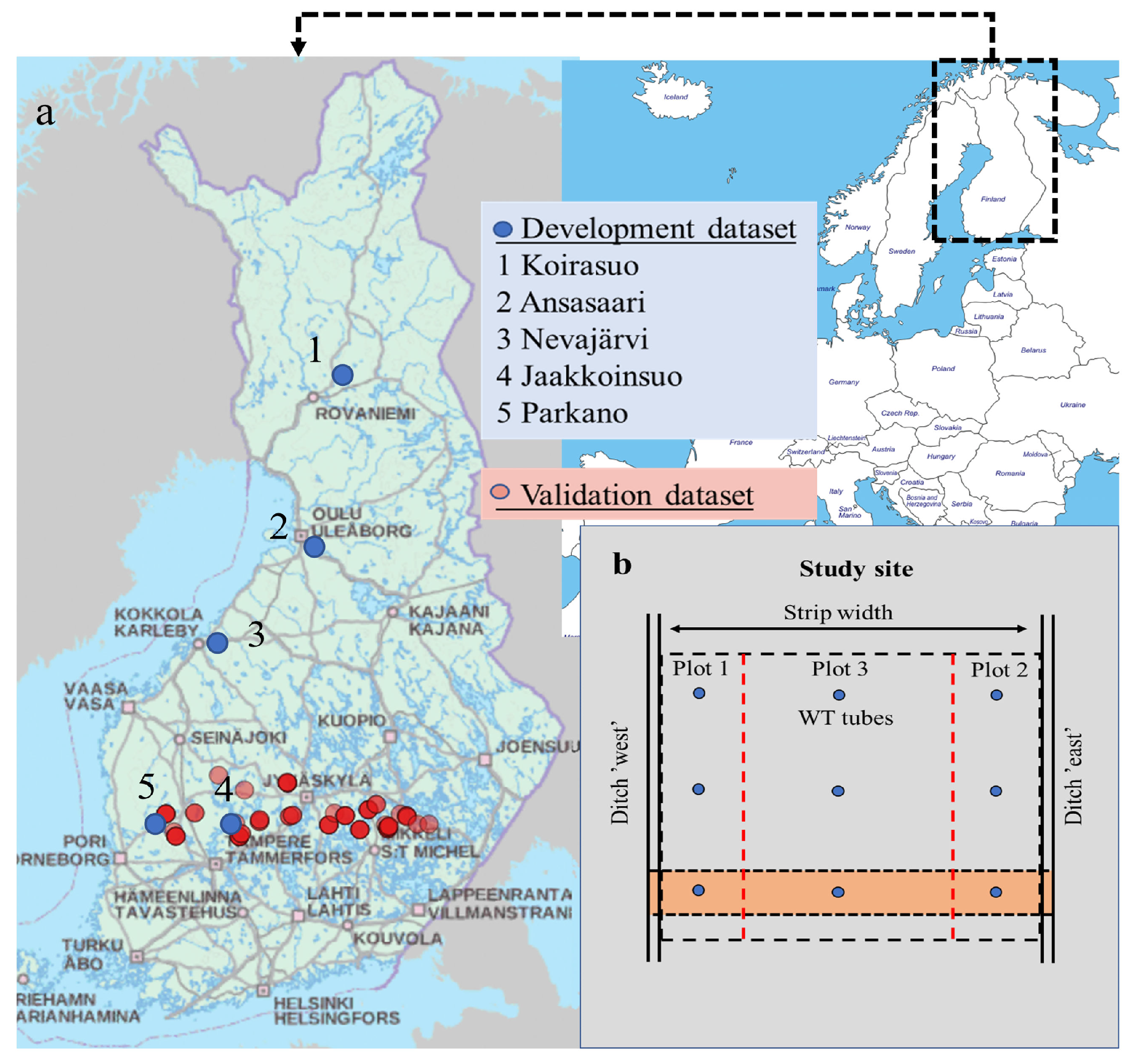
2.1. Data for Model Development

We used the data from an existing peatland forest water balance experiment [24] to evaluate the model structure through sensitivity analyses. Stand and site data, and five to eight years of $WT$ observations (monitored between 2007 and 2014) from five Scots pine (Pinus sylvestris L.) dominated peatland forests in Finland were used (Figure 1a: blue dots, $n_{sites}$ = 5, $n_{plots}$ = 11). The initial volume of stands ranged from 91 to 168 m³ ha⁻¹. The sites were drained >40 years ago with 25 to 65 m ditch spacing (

Table 1. Site properties in the development dataset; $n_{gs}$, number of growing seasons; $T_{sum}$, temperature sum degree days; $P_{annual}$, annual precipitation in mm; $A_{ini}$, initial stand age years; $V_{ini}$, initial stand volume in m³ ha⁻¹; $V_{end}$, stand volume at the end of the measuring period in m³ ha⁻¹; $sfc$, site fertility class; $H_{vonPost}$, degree of decomposition at the von Post scale; $D_{depth}$, ditch depth in m; $S_{width}$, strip width in m; ${WT}_{mean}$, mean observed water table in m; $n_{gwtubes}$, number of groundwater tubes. Peat types: LC = Wood-Carex peat, C = Carex peat, SC = Sphagnum-Carex peat, LS = Wood-Sphagnum peat, ErS = Eriophorum-Sphagnum peat.

Site	${\mathit{n}}_{\mathit{gs}}$	${\mathit{T}}_{\mathit{sum}}$	${\mathit{P}}_{\mathit{annual}}$	${\mathit{A}}_{\mathit{ini}}$	${\mathit{V}}_{\mathit{ini}}$	${\mathit{V}}_{\mathit{end}}$	sfc	Peat Type	${\mathit{H}}_{\mathit{vonPost}}$	${\mathit{D}}_{\mathit{depth}}$	${\mathit{S}}_{\mathit{width}}$	${\mathit{WT}}_{\mathit{mean}}$	${\mathit{n}}_{\mathit{gw}\mathit{tubes}}$
Koirasuo11	7	888	513	76	91	122	2	LC	4	−0.85	37	−0.39	3
Koirasuo12	7	888	513	76	123	164	2	LC	4	−0.85	37	−0.42	3
Ansasaari21	7	1106	497	39	140	187	3	SC…C	6	−0.45	40	−0.34	6
Ansasaari26	7	1106	497	39	110	141	3	SC…C	6	−0.45	40	−0.37	3
Nevajärvi11	8	1079	539	80	163	228	3	SC…LC	5	−1.04	25	−0.72	6
Nevajärvi14	8	1079	539	80	143	191	3	SC…LC	5	−1.04	25	−0.62	6
Nevajärvi31	8	1079	539	80	127	162	3	C	5	−1.08	25	−0.68	10
Nevajärvi34	8	1079	539	80	100	147	3	C	5	−1.08	25	−0.60	10
Jaakkoinsuo61	7	1195	523	86	144	173	5	LS…ErS	4–8	−0.85	40	−0.51	6
Jaakkoinsuo62	7	1195	523	86	149	187	5	LS…ErS	4–8	−0.85	40	−0.53	6
Parkano11	5	1176	614	130	168	192	5	LS…S	3–5	−0.86	65	−0.32	12

). Peat layer thickness varied from 0.6 m to >2.0 m.

The breast height diameter ($dbh$) of all trees and height (h) of sample trees were measured at the end of the experiment. Tree height at the beginning of the period was estimated by counting $n_{gs}$ (number of growing seasons, Table 1) internodes down from the top. The $dbh$ increment and the $dbh$ at the beginning of the study period were determined from drilled core chips. The initial stand volume ($V_{ini}$) and the volume at the end of the study period ($V_{end}$) were estimated from $dbh$ and h using volume equations [44]. The biomasses ($BM$) of bark, leaves, branches, stump, roots and stem at the beginning and the end of the period were determined using allometric equations [45].

$WT$ was measured manually from three to 12 groundwater tubes located in each sample plot (Table 1) on average once a week from spring to autumn when the water in the tubes was unfrozen. Site fertility class ($sfc$, fertility decreases from $sfc1$ towards $sfc6$, see [46,47], peat type, degree of decomposition using the von Post scale ($H_{vonPost}$, [48]), and ditch depth were determined on-site (Table 1). Strip width ($S_{width}$) was determined as a perpendicular distance between parallel ditches. Daily meteorological variables (precipitation P, air temperature $T_a$, global radiation $R_g$, and water vapor pressure $p_{H2O}$) for the research areas were obtained from the Finnish Meteorological Institute database in a 10 km × 10 km grid [49]. Photosynthetically active radiation ($PAR$) was considered to be 0.5 $R_g$.

2.2. Validation Data

SUSI was validated against an independent dataset consisting of 69 sample sites ($n_{sites}$ = 69) in central Finland, with each site containing three sample plots ($n_{plots}$ = 207) (Figure 1a, red dots,

Table 2. Mean measured stand characteristics (standard deviation in parentheses) of the validation dataset classified according to site fertility class ($sfc$, fertility decreases from $sfc2$ towards $sfc6$). Sites were measured in 1985 before onset of the growing season. Drain network dimensions and peat and stand characteristics were used in the parameterization and initialization of the Peatland simulator SUSI. The volume after five growing seasons ($V_{1984}$), the mean annual volume growth ($i_V$) and the median water table during the growing season of 1984 ($W{T}_{median}$) were used in testing the model performance.

Variable	Unit	$\mathit{sfc}2$	$\mathit{sfc}3$	$\mathit{sfc}4$	$\mathit{sfc}5$	$\mathit{sfc}6$
$n_{plots}$	number of plots	24	45	105	27	6
$n_{sites}$	number of sites	8	15	35	9	2
Used in in the initialization of SUSI-simulator validation runs
$D_{dept{h}_{w}est}$	m	−0.55 (0.14)	−0.49 (0.16)	−0.58 (0.16)	−0.57 (0.17)	−0.66 (0.11)
$D_{dept{h}_{e}ast}$	m	−0.61 (0.07)	−0.53 (0.16)	−0.59 (0.18)	−0.58 (0.15)	−0.65 (0.07)
$S_{width}$	m	48 (13)	59 (18)	53 (14)	57 (10)	50 (0)
${\rho }_b$	kg m−3	138.0 (29.0)	110.0 (26.0)	104.0 (28.0)	88.0 (25.0)	118.0 (11.0)
$pea{t}_N$	mg g−1	19.27 (2.57)	16.13 (3.75)	14.54 (3.32)	11.86 (2.69)	15.16 (1.19)
$pea{t}_P$	mg g−1	1.03 (0.33)	0.79 (0.34)	0.64 (0.15)	0.56 (0.16)	0.64 (0.08)
$pea{t}_K$	mg g−1	0.39 (0.08)	0.37 (0.1)	0.37 (0.08)	0.38 (0.08)	0.29 (0.05)
$n_{trees}$	trees ha−1	2017 (644)	1491 (547)	1389 (600)	1091 (321)	806 (282)
$H_{dom}$	m	13.5 (3.7)	9.6 (4.2)	7.8 (3.3)	6.7 (2.8)	5.1 (2.1)
$V_{1980}$	m3 ha−1	120.2 (58.2)	64.4 (58.0)	44.5 (31.8)	42.0 (22.0)	10.2 (4.7)
Used as a measured reference in the SUSI-simulator validation
$V_{1984}$	m3 ha−1	153.4 (65.5)	83.5 (63.3)	58.9 (39.0)	52.9 (26.3)	14.7 (7.0)
$i_V$	m3 ha−1 yr−1	6.64 (2.03)	3.82 (1.56)	2.87 (1.73)	2.18 (1.01)	0.89 (0.49)
$W{T}_{median}$	m, negative down	−0.58 (0.12)	−0.38 (0.16)	−0.35 (0.14)	−0.3 (0.13)	−0.24 (0.06)

). The sites were measured in spring 1985 and the peat characteristics have been reported by Laine and Vanha-Majamaa [50] and the stand characteristics by Hökkä et al. [51]. The data cover site fertility classes from $sfc$ 2 to 6. Currently, fertility classes from $sfc$ 2 to 5 are in active forestry use in Finland, whereas $sfc6$ is considered too infertile for wood production. Scots pine (Pinus sylvestris L.) was the dominant tree species in all sites. The mean annual temperature in the study region in 1980 to 1984 was +3.5 °C and the mean annual precipitation was 561 mm. The mean growing season (May–September) temperature was +12.3 °C and precipitation was 286 mm.

Each sample site was delineated by parallel ditches (Figure 1b). The sample site was further divided into three plots; plots 1 and 2 represented the area close to the ditch (plot center point located 5 m from the ditch) and plot 3 represented the midway between the two parallel ditches. Stand characteristics, including tree species, dominant height ($H_{dom}$), number of trees per hectare ($n_{trees}$), and the prevailing stand volume after the growing season of 1984 ($V_{1984}$) were measured at each plot (Table 2). The five-year annual volume growth ($i_V$) from 1980 to 1984 and the volume at the beginning of the growing season of 1980 were calculated using increment core samples [51]. The depth of the two delineating ditches (“west” [$D_{dept{h}_{w}est}$] and “east” [$D_{dept{h}_{e}ast}$]), peat bulk density (${\rho }_b$), peat type, and the peat N, P and K concentrations ($pea{t}_N$, $pea{t}_P$, $pea{t}_K$) of the topmost 0.2 m layer were determined. $WT$ was monitored during the growing season of 1984 in the three tubes installed at each sample plot. The experimental layout formed an ideal platform for testing the two-dimensional (2D) SUSI, which operates along a similar cross-section between two parallel ditches (Figure 2a). The ditches were named according to the 2D layout as the “west” and “east” ditches (Figure 1b) and do not necessarily refer to the real compass points in the field.

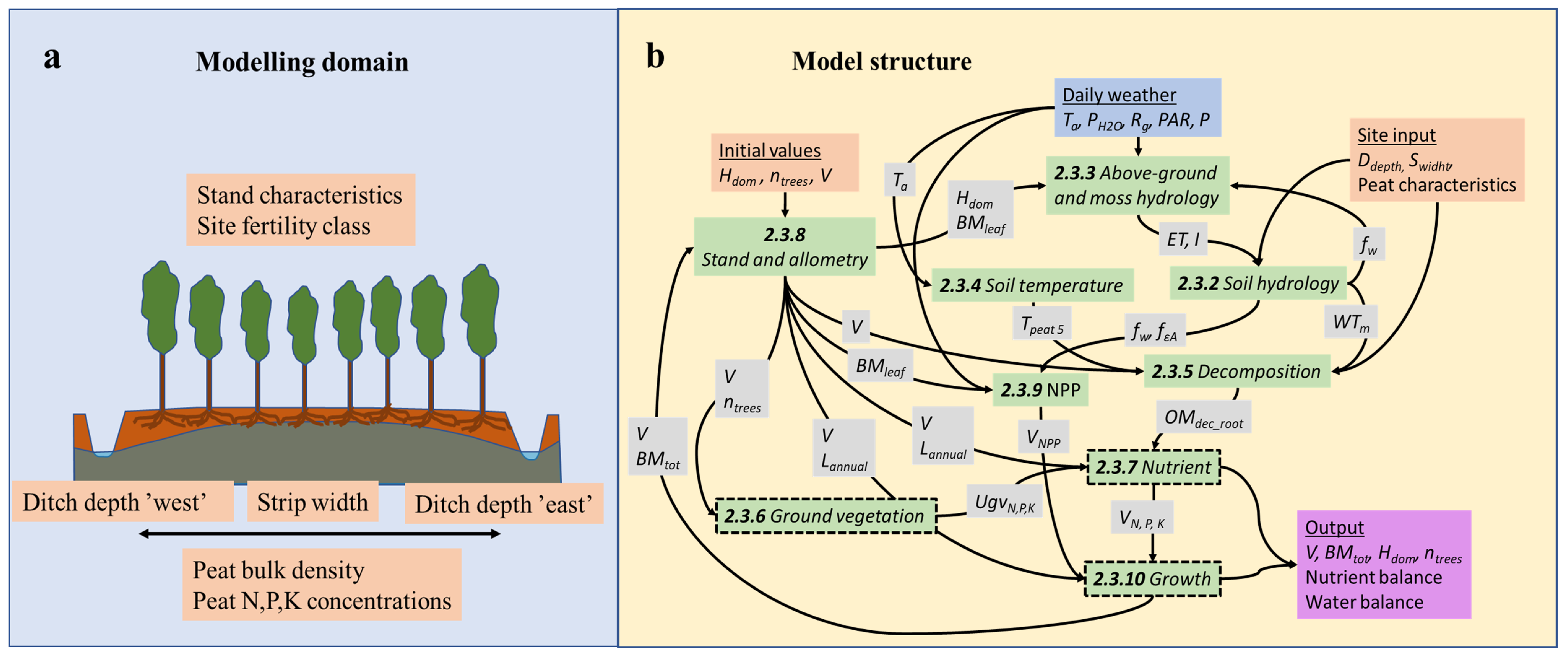
2.3. Peatland Simulator SUSI

2.3.1. General Description

SUSI describes hydrology, biogeochemical processes and stand growth along a 2D cross-section between two parallel ditches (Figure 2a). The structure of SUSI is modular (Figure 2b, modules in green boxes). Hydrology modules simulate above-ground and below-ground water fluxes and storages and compute daily $WT$. The peat temperature module simulates temperatures at different depths in the peat ($T_{peat}$). $WT$ and $T_{peat}$ affect the organic matter decomposition rate ($O{M}_{decroot}$) and the supply of nutrients. Furthermore, $WT$ directly controls net primary production ($NPP$) by scaling it down in case $WT$ is too high or too low ($f\left({ϵ}_A\right),f_w$). The nutrient balance module allocates the nutrient supply to stand, litter and ground vegetation, and together with the $NPP$ module they provide constraints for the stand growth module. The new stand volume follows Liebig’s law so that the new stand volume, at the end of the annual time step, is set to the minimum supported by $NPP$ ($V_{NPP}$) or by the supply of N, P or K ($V_{N,P,K}$). The new stand dimensions resulting from the growth are determined by allometric functions and have a feedback to the hydrology, decomposition, ground vegetation and NPP modules. The main computational loop uses a daily time step while the stand growth, ground vegetation and nutrient balance modules are updated annually. SUSI outputs include $WT$, stand growth rates, above-ground biomass and nutrient and water balance components. The model variables and their units are presented in Abbreviations.

2.3.2. Soil Hydrology Module: $WT$ Dynamics

Under dry conditions, $WT$ regulates growth directly through water limitation and under wet conditions by reducing the soil gas exchange due to low ${ϵ}_A$. These affect $NPP$ at daily time steps. Moreover, $WT$ controls the rate of organic matter decomposition and further the availability of nutrients. This effect is indirect and affects stand growth at the end of each simulation year. $WT$ is controlled by drainage design ($D_{depth}$ and $S_{width}$) and by stand characteristics that affect evapotranspiration ($ET$). Weather conditions and peat properties are factors that affect $WT$ but cannot be affected by management. A typical ditch network in Finland delineates rather narrow (30–50 m) and long (>200 m) strips in a fishbone pattern where $WT$ variation is largely governed by the distance to the closest ditch. Therefore, $WT$ dynamics, as affected by drainage, can be best described along a 2D cross-section extending from one ditch to another (Figure 2a).

SUSI thus simulates $WT$ for a cross-section between two parallel ditches. The computational domain is split in the horizontal direction into two-meter-wide soil columns. All inputs and outputs are given individually for each column. The solution of daily $WT$ follows a quasi-2D approach. The calculation of vertical water fluxes was simplified by assuming that a change in water storage in the peat column immediately affects $WT$, and that the water content above $WT$ achieves hydraulic equilibrium instantly [52]. The peat column was discretized into 0.05 m-thick layers with mid-point depths $z_i$ (in m). In the hydrological equilibrium, the water potential (${\mathsf{\Psi }}_i$, m H₂O) is the distance from $z_i$ to $WT$, and volumetric water content ($\theta$, m³ m⁻³) and ${ϵ}_A$ (m³ m⁻³) for each layer are calculated from ${\mathsf{\Psi }}_i$ and layer water retention characteristics [53]. The horizontal water movement is computed using the implicit solution of a diffusion equation (Equation (1)):

$$C_s\frac{\partial h_w}{\partial t}=\frac{\partial }{\partial x}\left(T_r\frac{\partial h_w}{\partial x}\right)+S,$$

(1)

where $C_s$ is the storage coefficient (m m⁻¹), $h_w$ is the height of the saturated water column (m), t is time (s), $T_r$ is transmissivity (m² s⁻¹), x is the horizontal distance (m), and S is a sink/source term (m s⁻¹) defined as the balance between the local infiltration and the $ET$ from the peat column. Transmissivity ($T_r$) was obtained by integrating the saturated hydraulic conductivity ($K_{sat}$, m s⁻¹) from the impermeable bottom to $WT$ (Equation (2)):

$$T_r\left(h_w\right)={\int }_{ib}^{h_w}{K}_{sat}dz,$$

(2)

where $ib$ is the depth of impermeable bottom (m) and z denotes the vertical direction. Prior to the simulation, $T_r$ values for different $h_w$ were computed at 0.01 m intervals and an interpolation function for $T_r\left(h_w\right)$ was constructed.

Water storage (W, m) in each peat column was obtained by integrating $\theta$ from the impermeable bottom to the soil surface (Equation (3)):

$$W\left(h_w\right)={\int }_{ib}^s\theta dz,$$

(3)

where s is the soil surface elevation (m). Prior to the simulation, $W\left(h_w\right)$ values were calculated at 0.01 m intervals and an interpolation function was constructed to describe the storage coefficient $C_s=d{h}_w/dW$ (m m⁻¹), i.e., the change in $WT$ with respect to the change in the profile of water storage. Likewise, an interpolation function was constructed to link $WT$ to the mean ${ϵ}_A$ for a given number of soil layers associated with the rooting zone.

We divided the peat column into 0.05 m layers and estimated saturated hydraulic conductivity ($K_{sat}$) and water retention characteristics from peat type and bulk density following Päivänen [54]. $K_{sat}$ values for the topmost 0.4 m layer were multiplied by 10 to account for the contribution of macropores and anisotropy in the rooting zone [55,56]. Constant head boundary conditions were applied in ditches when $WT$ in the strip was higher than the ditch bottom, whereas no flow condition was applied when $WT$ was below the ditch bottom level. The impermeable bottom was assumed to be at a depth of 1.5 m.

Daily $WT$ and rooting zone ${ϵ}_A$ were passed to the NPP module as nodewise input. The organic matter decomposition module requires the growing season (May–September)mean WT ($W{T}_m$) as input; therefore, soil hydrology was computed for one year at a time using a daily time step, and after each year, $W{T}_m$ was calculated. The daily decomposition could be simulated in a separate time loop after solving the hydrology.

2.3.3. Aboveground Hydrology Module: Infiltration and Evapotranspiration

The aboveground hydrology module provides the water sink/source term S (Equation (1)) for the soil hydrology module as the difference between infiltration (I) and $ET$ for each soil column (Figure 2b). The description and parameterization of the above-ground water budget was adopted from the spatial forest hydrology model SpaFHy [57]. The model describes rainfall and snow interception in the canopy and moss/litter layer, snow accumulation and melt, snow depth ($d_{snow}$), infiltration to soil, and $ET$. The $ET$ is computed according to a three-source model where plant transpiration and evaporation from the moss/litter layer and canopy interception storage are modeled separately using a Penman–Monteith equation [57]. For the transpiration, the canopy conductance depends on species-specific water use traits, the one-sided leaf-area index $LA{I}_{one}$ (m² m⁻²), environmental forcing and feedback from the root-zone moisture conditions (see [57]). Here, the moisture feedback is given as a Feddes-type restriction function $f_w$ (unitless), where canopy conductance (and thus transpiration) is reduced linearly when $WT$ is above −0.15 m or below −0.7 m [55]. Variations in transpiration rate across the peatland strip can occur in case $f_w$ becomes spatially variable.

The interception storages in the canopy and in the moss/litter layer are modeled using a bucket approach, where the water-storage capacities are proportional to $LA{I}_{one}$ and organic layer dry mass. The water content in these storages is increased by interception of rainfall/throughfall and decreased by evaporation [57]. The snowpack is described with a degree-day approach, where the snowmelt coefficient is a function of canopy closure resulting in a slower snowmelt in dense stands [58]. For stand description, the above-ground hydrology module requires information on canopy height, canopy closure, and $LA{I}_{one}$. The latter are derived here from stand basal area [59] and from stand leaf/needle mass using specific leaf area conversion factors [60]. Stand growth and management, such as tree species selection and harvesting, affect stand structure and then directly influence above-ground hydrology and $WT$.

2.3.4. Peat Temperature Module

Daily evolution of the peat temperature profile is computed using an explicit solution of a heat equation (Equation (4)):

$$\frac{\partial T_{peat}}{\partial t}=D_T\frac{{\partial }^2{T}_{peat}}{\partial x^2},$$

(4)

where $T_{peat}$ is peat temperature (°C) at depth z (m), t is time (s) and the thermal diffusivity $D_T$ is assumed to be constant (10⁻⁷ m² s⁻¹). This simplification is plausible for a range of water contents typical for peat soils with shallow $WT$ [61]. Annual mean air temperature of the simulation period was set as a constant lower boundary condition to the depth of three meters. The upper boundary condition was set equal to daily air temperature ($T_a$) when snow depth ($d_{snow}$) was zero, and to 0 °C otherwise. Peat temperature at the depth of 0.05 m ($T_{peat5}$) was passed as input for the organic matter decomposition module.

2.3.5. Organic Matter Decomposition Module

Heterotrophic respiration ($R_{het}$, g CO₂ m⁻² day⁻¹) and the mass of decomposed peat were computed at a daily time step after completing the hydrology calculation for each year. $R_{het}$ follows the empirical model of Ojanen et al. [5]:

$$R_{het}=R_{ref}^{B\left(\frac{1}{T{5}_{ref}-T{5}_0}-\frac{1}{T_{peat5-T{5}_0}}\right)},$$

(5)

where B (350) is the temperature sensitivity of respiration, $T{5}_{ref}$ is the reference soil temperature (10 °C), and $T{5}_0$ is the temperature at which respiration would reach zero (−46.02 °C). Following [5], we avoided extrapolation of Equation (5) by restricting $T_{peat5}$ to a maximum of +16 °C. Heterotrophic respiration at the reference soil temperature is calculated as:

$$R_{ref}=0.0695+3.7\ast {10}^{-4}V+5.4\ast {10}^{-4}{\rho }_b+1.2\ast {10}^{-3}W{T}_m,$$

(6)

where V is the stand volume (m³ ha⁻¹), ${\rho }_b$ is the peat bulk density (kg m³), and $W{T}_m$ is the mean growing season water table (m).

Mass of the decomposed organic matter ($O{M}_{dec}$) was estimated by converting $R_{het}$ from CO₂ to C and assuming a carbon content of 50% for decomposing organic material. Because $O{M}_{dec}$ is later used to approximate the release of nutrients, it is a relevant question how much of the organic matter decomposition and the subsequent nutrient release takes place in the rooting zone. Since the decomposition is predominantly an aerobic process, we assumed that the momentary $R_{het}$ is vertically distributed according to ${ϵ}_A$ profile. Prior to the simulation, an interpolation function was created connecting $WT$ to the relation: ${ϵ}_A$ in the rooting zone/total ${ϵ}_A$. The function was applied to daily $O{M}_{dec}$ and $WT$ to separate the decomposition in the rooting layer ($O{M}_{decroot}$). We used a rooting zone depth ($z_{root}$) of 0.4 m and studied the sensitivity of the model result to the rooting depth using the development dataset. $O{M}_{dec}$ and $O{M}_{decroot}$ were integrated to the annual time step and passed as a nodewise input to the nutrient module.

2.3.6. Ground Vegetation Module: Nutrient Demand

Ground vegetation competes with the tree stand for the available growth resources, especially for nutrients. The total above-ground biomass of ground vegetation, and the biomass in the bottom and field layers were calculated using empirical models, where the biomass depends on latitude, longitude, elevation, temperature sum, site fertility class, dominant tree species, stand volume, number of stems, basal area, stand age and drainage status (full models are given in Table 9 in [47]). Field layer biomass was divided into dwarf shrubs (90% in pine stands, 50% in spruce stands) and sedges and herbs (10% in pine stands, 50% in spruce stands). The above-ground biomass in the field layer was multiplied by 1.7 to account for root biomass and to obtain the total field layer biomass. The bottom layer was assumed to be formed of Sphagnum and other mosses without roots. Thus, the accounted ground vegetation components were i = [dwarf shrubs, herbs and sedges, mosses]. Nutrient content in component i ($cg{v}_{N,P,K}^i$, kg ha⁻¹) was obtained by multiplying the biomass ($BMg{v}^i$, kg ha⁻¹) with nutrient concentrations ($ng{v}_{N,P,K}^i$, mg g⁻¹) adopted from [62]:

$$cg{v}_{N,P,K}^i=BMg{v}^i\ast ng{v}_{N,P,K}^i\ast 1000.$$

(7)

Giving the stand characteristics at times $t_1$ and $t_2$ to the ground vegetation model and applying Equation (7) enables the description of the net change in ground vegetation biomass ($\Delta BMg{v}^i$) and nutrient content ($\Delta cg{v}_{N,P,K}^i$) during the period.

In terms of nutrient consumption, the nutrient turnover connected to annual growth and litterfall is more important than the net change in the ground vegetation biomass [63]. Following Mälkönen [63], we assumed an annual turnover ($tog{v}^i$, yr⁻¹) of 0.2, 0.5 and 0.3 of total biomass for dwarf shrubs, herbs and sedges, and mosses, respectively. The annual ground vegetation litterfall ($Lg{v}^i$, kg ha⁻¹ yr⁻¹) was therefore:

$$Lg{v}^i=tog{v}^i\ast BMg{v}^i.$$

(8)

where $Lg{v}^i$ is mass lost in litter and replaced by growth every year. Before the litterfall, dwarf shrubs and herbs retranslocate a share of nutrients to be reused in the new growth (Abbreviations). The total nutrient uptake demand ($Ug{v}_{N,P,K}^i$, kg ha⁻¹ yr⁻¹) was obtained as:

$$Ug{v}_{N,P,K}^i=\Delta cg{v}^i+\left(1-rg{v}_{N,P,K}^i\right)\ast ng{v}_{N,P,K}^i\ast Lg{v}^i,$$

(9)

where $rg{v}_{N,P,K}^i$ is the share on retranslocated nutrients. The sum of the annual nutrient uptake demand of all ground vegetation components ($Ug{v}_{N,P,K}$) was passed as input to the nutrient module. The ground vegetation leaf mass ($BMg{v}_{leaf}$, kg ha⁻¹) was obtained by multiplying $BMg{v}^i$ by 0.2, 0.5 and 0.3 of total biomass for i = dwarf shrubs, herbs and sedges, and mosses, respectively. $BMg{v}_{leaf}$ was passed as input to the nutrient module.

2.3.7. Nutrient Module: Release, Allocation and Uptake of Nutrients

The nutrient module calculates nutrient supply, allocates it to stand growth, litterfall and ground vegetation, and finds the maximum stand growth supported by the nutrient supply. It receives $O{M}_{dec}$ and $O{M}_{decroot}$ as input from the organic matter decomposition module, and stand volume (V), annual litterfall ($L_{annual}$) and stand leaf mass ($B{M}_{leaf}$) from the stand and allometry module, and nutrient uptake demand of ground vegetation ($Ug{v}_{N,P,K}$) and ground vegetation leaf mass ($BMg{v}_{leaf}$) from the ground vegetation module. Annual nutrient supply in the rooting zone ($s_{N,P,K}$, kg ha⁻¹yr⁻¹) was obtained as follows:

$$s_{N,P,K}=O{M}_{decroot}\ast \left(1-Im{m}_{N,P,K}\right)\ast pea{t}_{N,P,K}/1000\ast D_{N,P,K},$$

(10)

where $pea{t}_{N,P,K}$ is the peat nutrient concentration (mg g⁻¹), $D_{N,P,K}$ is annual atmospheric deposition (5.0, 0.12 and 0.50 kg ha⁻¹ yr⁻¹ for N, P and K, respectively, [64,65]), $Im{m}_{N,P,K}$ is the fraction of released nutrients that become immobilized by microbial biomass (0.9, 0.8 and 0.0 for N, P and K, respectively, see, e.g., [66]). Substituting $O{M}_{decroot}$ with ($O{M}_{dec}$–$O{M}_{decroot}$) in Equation (10) we obtained the nutrient release below $z_{root}$, which we assumed to leach ($leac{h}_{N,P,K}$, kg ha⁻¹ yr⁻¹) to the water course. We measured $pea{t}_{N,P,K}$ available for the validation dataset (Table 2), and for the development dataset we used mean $pea{t}_{N,P,K}$ values for different site fertility classes [67,68].

The nutrient supply $s_{N,P,K}$ was allocated to the use of the stand and ground vegetation in proportion to their green mass:

$$gvshare=\frac{BMg{v}_{leaf}}{BMg{v}_{leaf}+B{M}_{leaf}},$$

(11)

where $gvshare$ is the maximum share of nutrient supply received by the ground vegetation. The ground vegetation receives ($Upg{v}_{N,P,K}$, kg ha⁻¹ yr⁻¹):

$$Upg{v}_{N,P,K}=min\left(gvshare\ast s_{N,P,K},Ug{v}_{N,P,K}\right),$$

(12)

The amount of nutrients that the tree stand loses in the litterfall ($L_{N,P,K}$, kg ha⁻¹yr⁻¹) was calculated considering nutrient retranslocation from the senescing tissues and the maximum allowed share from the nutrient release:

$$L_{N,P,K}=min\left(\left(1-r_{N,P,K}\right)L_{annual},\frac{(1-gvshare)}{2}{s}_{N,P,K}\right),$$

(13)

where $r_{N,P,K}$ is the share of retranslocated nutrients (kg kg⁻¹) that were set to 0.69, 0.73 and 0.80 for N, P and K, respectively [69]. Thus, the nutrient supply available for the stand growth ($s_{standgrN,P,K}$, kg ha⁻¹year⁻¹) was:

$$s_{standgrN,P,K}=s_{N,P,K}-Upg{v}_{N,P,K}-L_{N,P,K}.$$

(14)

We solved the potential stand volume growth facilitated by $s_{standgrN,P,K}$ for the time interval $t_1$, $t_2$. First, the stand nutrient content for the beginning of the time interval was computed from the stand volume $V\left(t_1\right)$ as [65]:

$$c_{N,P,K}=exp\left(lna+b\ast ln\left(V\right)+k\right),$$

(15)

where $c_{N,P,K}$ is N,P and K content in the stand (kg ha⁻¹), V is the stand volume (m³ ha⁻¹), and lna, b and k are species-wise and nutrient-wise parameters (see [65]). Now we can solve the new volume of the growing stock allowed by the supply of nutrients that are available for stand growth ($s_{standgrN,P,K}$):

$$V_{N,P,K}=exp\left(\left(ln\left(c_{N,P,K}+s_{standgrN,P,K}\right)-lna-k\right)/b\right),$$

(16)

where $V_N$, $V_P$, $V_K$ are the potential stand volumes allowed by the supply of N, P and K (m³ ha⁻¹), $c_{N,P,K}$ is the stand nutrient content in t1 (kg ha⁻¹), and lna, b and k are species-wise and nutrient-wise parameters [65]. $V_N$, $V_P$ and $V_K$ were passed as input to the growth module.

2.3.8. Stand and Allometry Module: Allometry and Growth Path

Biomass allometry and the initial state of the stand were processed from standard stand-wise forest inventory data using the empirical growth and yield model Motti [46,70]. The stand was initialized using stocking ($n_{trees}$), volume (V), age (A), dominant height ($H_{dom}$) and tree species ($S_p$). From the given information, Motti compiles stand diameter distribution, applies the biomass equations by Repola [45], and calculates the leaf ($B{M}_{leaf}$), bark, branch, stem, coarse root and fine root biomass. The stand total biomass ($B{M}_{tot}$) is the sum of the biomass components. $L_{annual}$ was derived from the biomass and the mean longevity of the biomass components (4, 22 and 1 years for leaf, branch, and fine roots, respectively [71,72]). The biomass yield ($B{M}_{yield}$) for the time interval $t_1$, $t_2$ (in years) was obtained as ($B{M}_{tot}\left(t_2\right)-B{M}_{tot}\left(t_1\right))+(t_2-t_1)L_{annual}$. The Motti outputs were also used to construct the allometric development path for the stand by building interpolation functions between $B{M}_{yield}$, $B{M}_{tot}$, $B{M}_{leaf}$, $H_{dom}$, $L_{annual}$ and V. The application of the interpolation functions allowed us to decouple time from Motti results and to drive the stand development through either $NPP$ or the growth allowed by the nutrient supply. Thus, Motti provides the allometric road map for stand development, but growth rate is now governed by environmental factors.

2.3.9. Net Primary Production Module: $NPP$

We calculated the net primary production ($NPP$) using the method described by Mäkelä et al. [73]. The method applies light use efficiency, all-sided leaf area, and daily meteorological variables:

$$NPP=f_{NPP}\beta \left(1-e^{-k_{ext}LA{I}_{all}}\right){\Phi }_k\prod _i{f}_{ik},$$

(17)

where $NPP$ is the net primary production (g C m⁻² d⁻¹), $f_{NPP}$ is the fraction of net primary production from gross primary production ($f_{NPP}$ = 0.5, see [74]), $\beta$ is the potential daily light use efficiency ($LUE$, g C mol⁻¹), $k_{ext}$ is the Beer–Lambert light extinction factor ($k_{ext}$ = 0.2), $LA{I}_{all}$ is the all-sided leaf area calculated from leaf mass and specific leaf area [60], ${\Phi }_k$ is $PAR$ (mol m⁻² d⁻¹) and $f_i$ [0,1] are modifying factors for suboptimal conditions including a light modifier, a temperature modifier, a vapor pressure deficit modifier and a soil water content modifier (see [73]). We added an extra modifier that linearly reduces $NPP$ when ${ϵ}_A$ in top peat layers decreases from 0.06 to 0 m ³ m⁻³ [30]. The three upmost peat layers, equivalent to 0.15 m, were accounted for in the evaluation of ${ϵ}_A$. The effect of the number of layers was tested using the development dataset and is included in the sensitivity analysis of SUSI. Otherwise, the parameterization of Equation (17) follows Table 2 in [73], column “Whole data”. $NPP$ was calculated at daily time steps and was integrated into an annual time step ($NP{P}_{annual}$), which was used to derive the potential growth level. The new potential total biomass ($B{M}_{tott+1}$) was obtained as:

$$B{M}_{tott+1}=B{M}_{tot}+NP{P}_{annual}-L_{annual}.$$

(18)

$B{M}_{tott+1}$ was converted to stand volume using the interpolation function between stand total biomass and stand volume. The new potential stand volume allowed by $NPP$ ($V_{NPP}$, m³ ha⁻¹) is passed as input for the growth module.

2.3.10. Growth Module: Biomass Growth and Yield

The growth module receives the following four different volume suggestions: $V_{NPP}$ based on photosynthesis and respiration, and $V_N$, $V_P$ and $V_K$ based on the nutrient supply. Based on Liebig’s law of minimum, the new stand volume is min($V_{NPP}$, $V_N$, $V_P$, $V_K$). The new stand total biomass ($B{M}_{tot}$) was solved using the interpolation function between stand volume and stand biomass. $B{M}_{leaf}$ and $H_{dom}$ were updated after each simulation year.

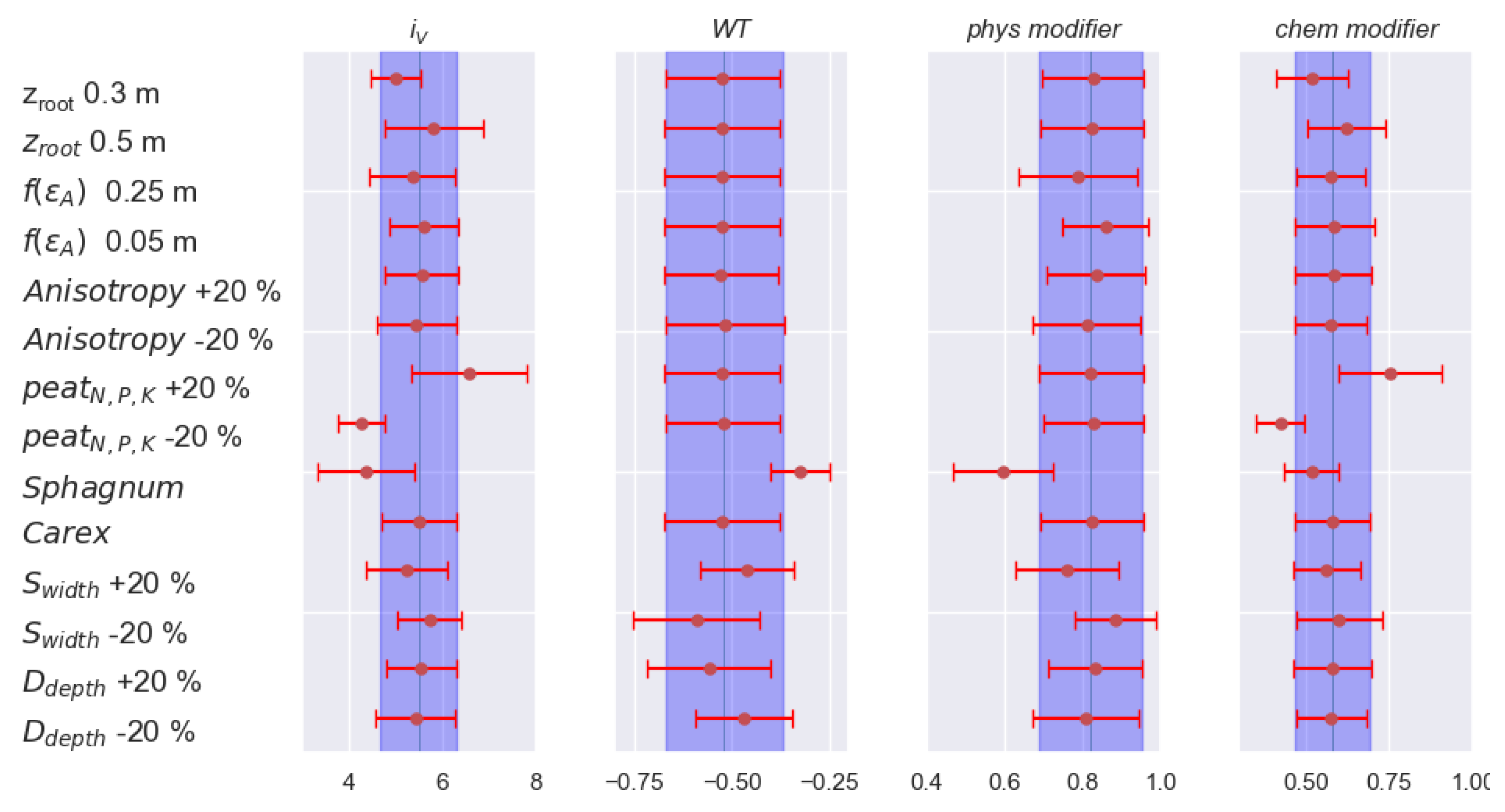
2.4. Sensitivity Analysis

We studied the sensitivity of the model results (i) for such model structures that are difficult to quantify experimentally ($z_{root}$, $f\left({ϵ}_A\right)$, anisotropy), (ii) to identify characteristics that may not be directly available in the forest inventory data ($pea{t}_{N,P,K}$, peat type), and (iii) to identify drainage options ($D_{depth}$, $S_{width}$) that can be managed in practical forestry. The baseline for the sensitivity analysis was obtained by running SUSI for the development dataset that includes 11 stands, and by computing the resulting means and standard deviations over the sites. Then we systematically modified the model structures and parameters, applied the model, and compared the result mean and standard deviation to the baseline. Nutrients released in the rooting layer (z > $z_{root}$) become available for stand growth (Section 2.3.5), whereas below $z_{root}$ the nutrients are assumed to leach to the water course (Section 2.3.7). In the model application, $z_{root}$ was set to 0.4 m, and in the sensitivity analysis values of 0.3 and 0.5 m were tested. We also tested the effect of the depth with the ${ϵ}_A$ modifier (Section 2.3.9). The baseline depth for the $f\left({ϵ}_A\right)$ was 0.15 m, and in the sensitivity analysis we tested the depths of 0.05 and 0.25 m. In the sensitivity analysis, anisotropy (Section 2.3.2), $D_{depth}$, $S_{width}$ and $pea{t}_{N,P,K}$ were increased or decreased by 20% from the baseline/observed value. The effect of peat characteristics was studied by applying Sphagnum or Carex peat for the development dataset.

2.5. Model Application to Ditch Network Maintenance

A typical case of ditch network maintenance (DNM) was used as an example of model application in practical decision making in peatland forestry. In the reference scenario, $D_{depth}$ was −0.3 m, corresponding to deteriorated ditches due to sedimentation and ingrowth of vegetation. In the DNM scenario with cleaned ditches, $D_{depth}$ was deepened to −0.9 m. Other site input variables were kept the same as in the model validation runs. The five-year growth response $\Delta i_{V5}$ (m³ ha⁻¹) was obtained as a volume growth difference between scenarios with −0.9 and −0.3 m ditch depths. The simulated growth response was compared to values published in previous studies.

3. Results

3.1. Model Development and Sensitivity

The simulated $WT$ followed the observed temporal dynamics of $WT$ in the development sites (Figure 3). The development data covered a wide range of climate, site and hydrological conditions across Finland (Figure 1a). Highest $WTs$ (−0.1–−0.2 m) were observed in the beginning of the growing season, whereas the lowest $WTs$ (−0.5–−0.9 m) occurred in July–August. The model predicted reasonably well the mean $WTs$ in July–August (RMSE 0.15 m, Figure 4a), which is the key period for stand growth.

The correlation between the observed and modeled biomass growth was high (r = 0.79) in the development dataset (Figure 4b), where the observed biomass growth ranged between 5000 and 9000 kg ha⁻¹ yr⁻¹. The northernmost site had the lowest growth rate. The model predicted the biomass and the volume growth well with a small bias (Figure 4b,c) and the RMSE of the volume growth prediction was 1.08 m³ ha⁻¹ yr⁻¹.

The simulations suggested that in the southernmost site (Parkano11) the potential biomass growth with no physical or chemical growth restrictions ranged between 9470 and 11,500 kg ha⁻¹ yr⁻¹ during the five simulated years. The physical growth restrictions, i.e., inadequate $O_2$ supply or drought, decreased the growth rate to 7090–9700 kg ha⁻¹ yr⁻¹. Introducing the chemical growth restrictions, i.e., inadequate nutrient supply, decreased the growth rate further to the level of 5700–6100 kg ha⁻¹ yr⁻¹. In the northernmost site (Koirasuo11), the potential growth rate was 6820–7470 kg ha⁻¹ yr⁻¹, while the growth rate allowed by physical and chemical restrictions were 5380–7100 kg ha⁻¹ yr⁻¹ and 2730–5550 kg ha⁻¹ yr⁻¹, respectively. In the development dataset, the simulated leaching rates of N, P and K to water courses were 2.12 (range 0.3–4.2), 0.15 (range 0.02–0.32) and 0.26 (range 0.04–0.53) kg ha⁻¹ yr⁻¹, respectively.

Sensitivity analysis indicated that the stand growth was most sensitive to peat nutrient contents and to peat type (Figure 5). Higher peat nutrient content increased the value of chemical growth modifiers and therefore markedly increased the stand growth. The physical growth modifier was reflected in the fact that a peat profile consisting of pure Sphagnum peat decreased the stand growth through a substantially higher $WT$ compared with Carex peat. Drainage management had a slightly smaller effect on the stand growth than peat type: $S_{width}$ lowered $WT$ more than $D_{depth}$ and affected the growth by slightly increasing the value of both the physical and chemical growth modifiers. The parameters connected to model structure had a small effect on the stand growth.

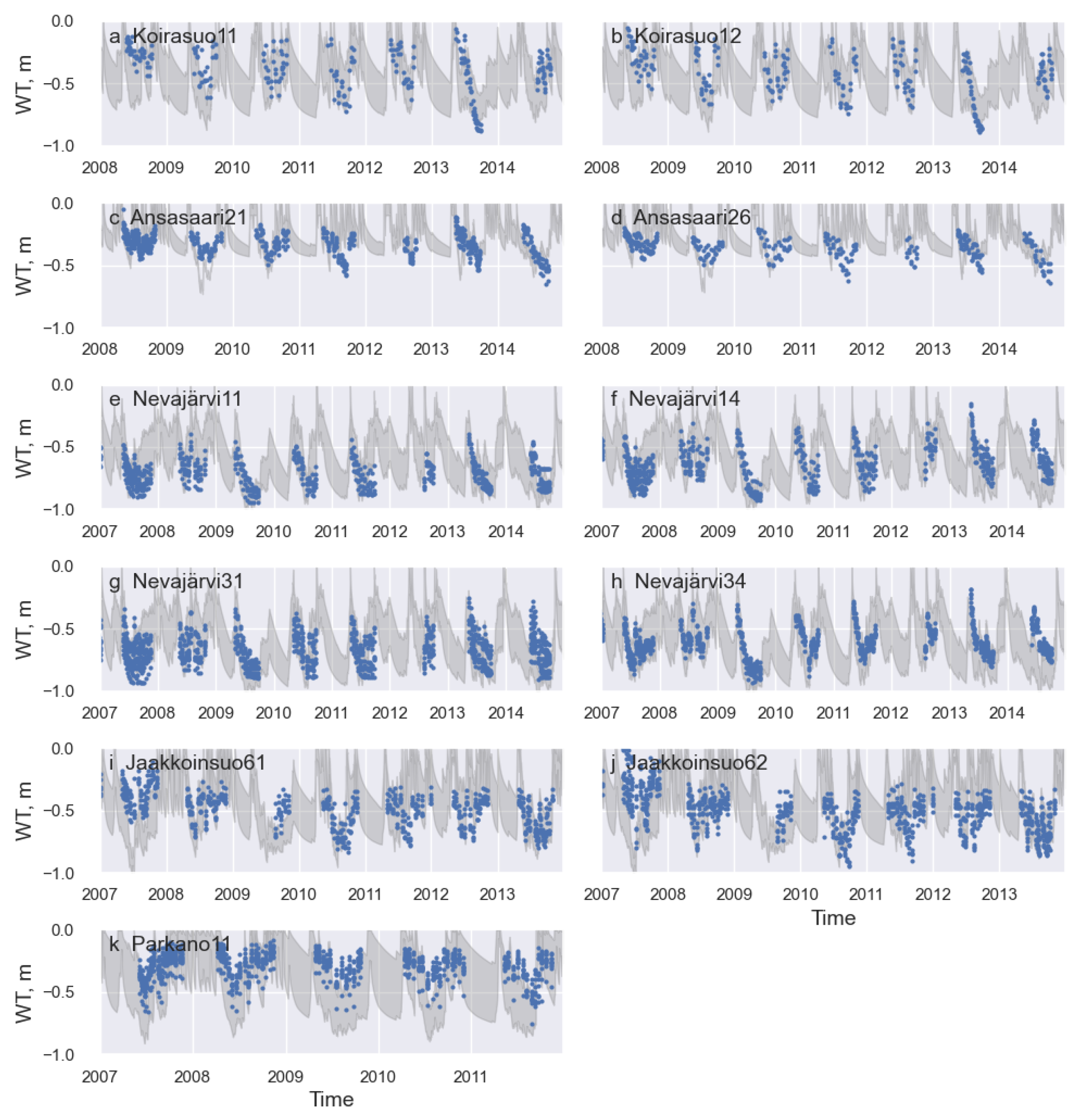
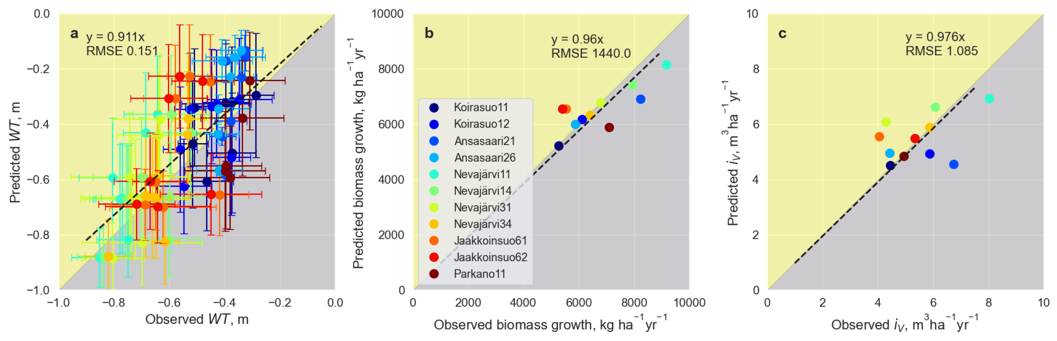
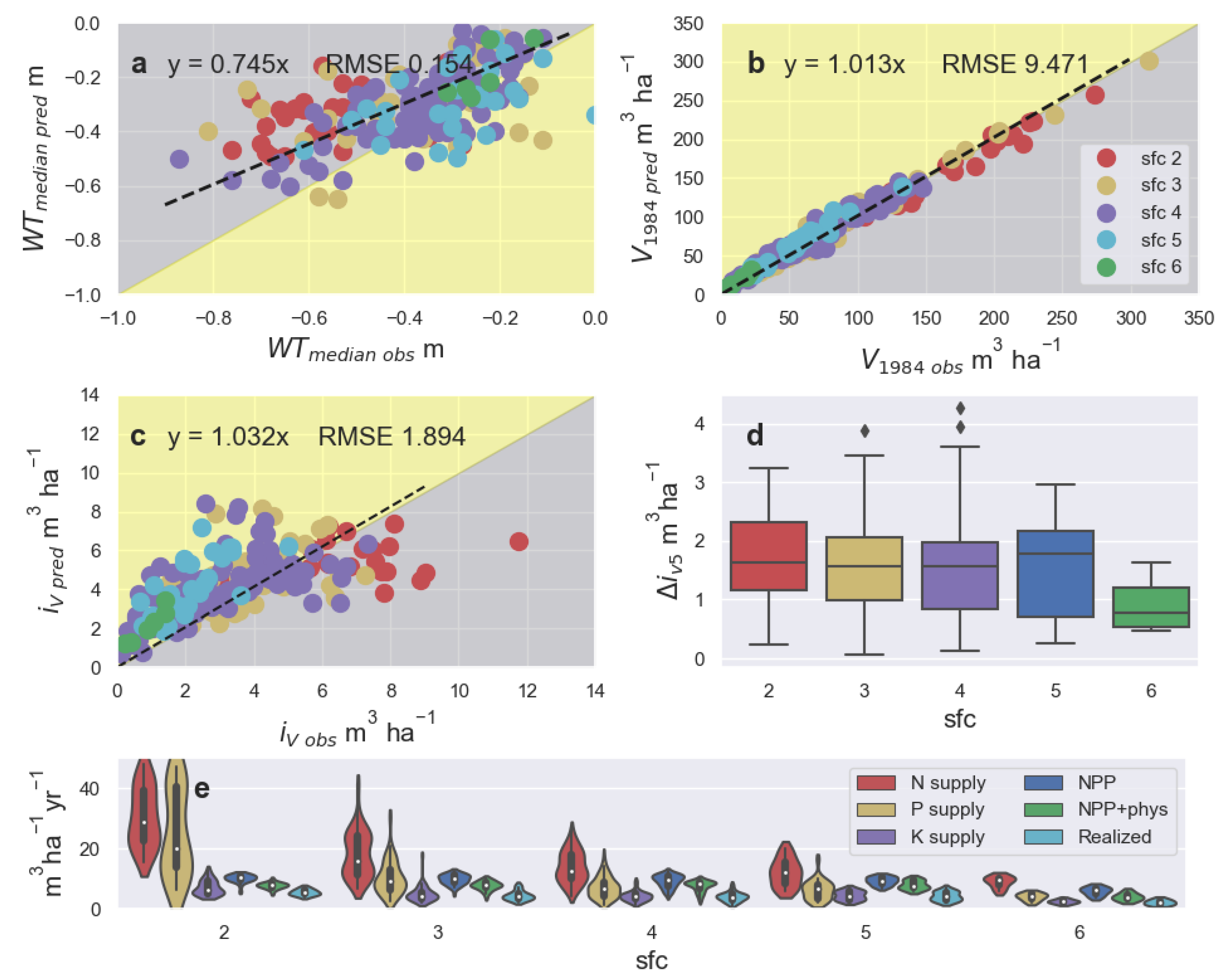
3.2. Model Validation and Application to Ditch Network Maintenance

Our validation data covered all site fertility classes that are under forest management in Finland, with the exception of $sfc1$, which is the most productive, generally thin-peated, Norway spruce-dominated site class (Table 2). The data also covered a large range of $V_{ini}$, $D_{depth}$, $S_{width}$ and peat characteristics (Table 2, Figure 6b). SUSI was able to predict the growing season $WT$ with reasonable accuracy. Only in case of the $sfc2$, the model produced too high $WT$ (Figure 6a), which resulted in an underestimation of stand growth (Figure 6c). In $sfc2$, the peat bulk density was considerably higher than in the other site fertility classes (Table 2). Otherwise, the predicted and observed iv5 (Figure 6c) followed the 1:1 line, indicating the low bias and sound functioning of the model. The absolute value of the residuals tended to increase towards the higher volume growth.

SUSI was applied to all validation sites to demonstrate the growth response to deepening the ditches by DNM from −0.3 to −0.9 m. The change in five-year volume growth ($\Delta i_{V5}$) was lowest for the most infertile sites (Figure 6d). For fertile and medium fertile sites, the average $\Delta i_{V5}$ was slightly less than 2 m³ ha⁻¹ over five years, the upper range being 3.5 m³ ha⁻¹. Further analysis of the model results revealed that the supply of N and P increased towards fertile sites, while K supply remained relatively constant and was low in fertile sites compared with N and P, causing K supply to become the main chemical growth-limiting factor (Figure 6e). Growth was mostly limited by the chemical limit introduced by inadequate K supply but sometimes also by physical constraints (Figure 6e).

4. Discussion

We constructed a unique peatland forest simulator named SUSI that mechanistically addresses the effects of drainage design (ditch depth and strip width) on the stand growth response under dynamic weather conditions and with differing stand characteristics, peat types and site fertility classes. SUSI was able to predict the $WT$ and stand growth with good accuracy in the validation data, which covered a large range of site fertility classes, initial stand volumes, ditch depths, strip widths and peat characteristics (Figure 6, Table 2). In $sfc2$, however, the model predicted too high $WT$, and consequently underestimated the stand growth. This can be due to its high peat bulk density (Table 2), which may have resulted in an underestimation of its hydraulic conductivity. In the upper part of the peat profile the hydraulic conductivity can be dominated by macropores and root channels, which enable more efficient water movement than was expected in the model on the basis of the high-density soil matrix (see, e.g., [55]). These macropores may facilitate more efficient drainage, lower $WT$, and better stand growth than realized in our model. The model results were most sensitive to site characteristics, such as peat nutrient contents and peat type (Figure 5), and less to model structure. This indicates that the model can be applied robustly to different sites provided that careful attention is paid to site description and derivation of soil characteristics.

Process-based modeling of hydrology and biogeochemistry enables the identification of different growth-limiting factors. The sensitivity analysis suggested that the physical growth restriction (oxygen stress) most likely occurs in Sphagnum peats, where $WT$ tends to be high due to low hydraulic conductivity. The validation dataset revealed that the chemical growth restriction was mostly attributable to availability of K (Figure 6). Previous studies have demonstrated that tree growth in peatlands is frequently limited by K and/or P availability, and only at infertile sites by N availability [32,33,34]. K deficiency is among the most common nutritional disorders in forested peatlands [33], because K stores in peat are low [32,68], K concentration in peat decreases over time due to drainage [68], K is poorly retained in soil [75] and is easily leachable [76]. The probability of K deficiency increases following consecutive harvestings [34,77] and can be counteracted by fertilization with, e.g., wood ash [78,79].

We demonstrated the use of SUSI for ditch network maintenance. The modeled growth responses to deepening the ditches from −0.3 to −0.9 m varied between 0.5 and 3.5 m³ ha⁻¹ over five years (Figure 6a). The most infertile sites had the mean growth response of 0.75 m³ ha⁻¹ in five years, whereas the growth response for the more fertile sites was slightly less than 2 m³ ha⁻¹ in five years. These values are close to the 1 to 4 m³ ha⁻¹ range observed in empirical studies for boreal drained peatland forests [80,81,82].

According to SUSI, DNM lowers $WT$, which improves the aeration in the rooting zone, but above all, increases the decomposition of organic matter and thereby the availability of nutrients. This induces the stand growth response. Several field experiments have demonstrated that drainage improves nutrient availability in peat [83,84,85,86], and improved nutrient availability is known to enhance the growth rate of trees [27,87,88].

Given that the growth response to drainage in the drained sites is mostly induced by improved nutrient supply [83], drainage can be considered as an act to increase nutrient supply comparable to fertilization. Due to low K concentration in peat, a large volume of peat must be subject to decomposition to produce a unit volume of timber. In the studied stands, increasing stand volume by 1 m³ requires 0.23 to 0.33 kg K according to the nutrient equations presented by Palviainen and Finér [65]. With the given peat K concentrations (Table 2), decomposition of 500 to 1100 kg of peat would facilitate the growth of 1 m³. Because of the differences in the peat and wood K stoichiometry, we can conclude that drainage is an inefficient way to supply K to the tree stand. This is supported by the low growth responses observed in previous studies after deepening of ditches by DNM [81]. Because of the K deficiency, an excess amount of mineralized N and P with respect to stand demand remains in the soil and is at risk of being exported to water courses. This can be seen in drained forested peatlands as chronic high exports of N [7]. This nutritional imbalance also weakens carbon sequestration, because the site $NPP$ cannot reach the levels otherwise enabled by the leaf mass and light availability.

SUSI facilitates a search for more efficient and environmentally feasible methods of peatland management. Our results suggest that increasing nutrient supply by fertilization may be a more efficient means of increasing and maintaining tree growth than lowering $WT$ by drainage. By avoiding drainage, we can also avoid the exports of suspended solids and nutrients that are caused by drainage. Peatland fertilization with wood ash has not been observed to significantly increase nutrient exports to water courses [79,89]; therefore, managing site nutrition by fertilization instead of drainage may be a valid strategy to mitigate adverse environmental effects whilst still maintaining the stand productivity. Nutrient balance computation in SUSI facilitates estimation of N, P and K leaching to water courses. Our datasets did not involve estimates of nutrient leaching; however, the simulated values were close to those reported for drained peatlands: 3–4.5 kg N ha⁻¹ yr⁻¹, 0.12–0.15 kg P ha⁻¹ yr⁻¹ [90] and 0.6–2.6 K ha⁻¹ yr⁻¹ [34]. Although nutrient leaching was not the main scope of this study, this comparison provides independent support for the nutrient balance simulation in SUSI. A more profound development of nutrient export simulation will be the scope of a future study.

As SUSI provides a direct link between the stand growth and drainage design, it can be used, e.g., in cost–benefit analyses connected to DNM under current and projected climates. The analysis enables discarding economically unfeasible sites from the DNM plans, that is, sites that would only produce adverse environmental effects without any economic gain. Because nutrient dynamics have a central role in growth response, SUSI can also be used to design fertilization schemes to replace DNM with a suitable fertilization regime and thereby increase the profitability of peatland forestry and mitigate the adverse environmental effects. Continuous-cover forestry has been proposed as an option to ameliorate the adverse effects of peatland management [91]. Since there is currently little experimental data from continuous-cover management in drained peatlands, SUSI can be a particularly useful tool to support decision making. In addition, as a process-based model, SUSI can be applied in the search for peatland management schemes under predicted drier growing seasons and elevated temperatures connected to changing climate. The current version of SUSI can be safely applied southwards from the areas included in this study, as long as the tree allometry [45] and the peat CO₂ emission models [5] remain valid, which extends at least to the southern coast of Finland. However, the modular structure of SUSI enables the user to substitute model components with locally valid model components. In these cases, the model framework still remains valid. Because of its open-source code (Python 3.7), modular structure, and the fact that it realistically accounts for essential processes such as hydrology, nutrient balance, and stand growth, SUSI also provides a good platform for further development. The next development stages may include the addition of economic cost–benefit analyses, greenhouse gas emissions and the computation of nutrient exports to water courses.

References

1. Renou-Wilson, F.; Bolger, T.; Bullock, C.; Convery, F.; Curry, J.; Ward, S.; Wilson, D.; Müller, C. BOGLAND - Sustainable Management of Peatlands in Ireland; Environmental Protection Agency: Washington, DC, USA, 2011; p. 157. [Google Scholar]
2. Päivänen, J.; Hånell, B. Peatland Ecology and Forestry—A Sound Approach; Helsingin yliopiston metsätieteiden laitoksen julkaisuja; Helsingin Yliopiston Metsätieteiden Laitos: Helsinki, Finland, 2012. [Google Scholar]
3. Xu, J.; Morris, P.J.; Liu, J.; Holden, J. PEATMAP: Refining estimates of global peatland distribution based on a meta-analysis. CATENA 2018, 160, 134–140. [Google Scholar] [CrossRef] [Green Version]
4. Minkkinen, K.; Laine, J. Long-term effect of forest drainage on the peat carbon stores of pine mires in Finland. Can. J. For. Res. 1998, 28, 1267–1275. [Google Scholar] [CrossRef]
5. Ojanen, P.; Minkkinen, K.; Alm, J.; Penttilä, T. Soil–atmosphere CO2, CH4 and N2O fluxes in boreal forestry-drained peatlands. For. Ecol. Manag. 2010, 260, 411–421. [Google Scholar] [CrossRef]
6. Jauhiainen, J.; Hooijer, A.; Page, S.E. Carbon dioxide emissions from an Acacia plantation on peatland in Sumatra, Indonesia. Biogeosciences 2012, 9, 617–630. [Google Scholar] [CrossRef] [Green Version]
7. Nieminen, M.; Sallantaus, T.; Ukonmaanaho, L.; Nieminen, T.M.; Sarkkola, S. Nitrogen and phosphorus concentrations in discharge from drained peatland forests are increasing. Sci. Total Environ. 2017, 609, 974–981. [Google Scholar] [CrossRef]
8. Boggie, R.; Miller, H.G. Growth of Pinus contorta at Different Water-Table Levels in Deep Blanket Peat. For. Int. J. For. Res. 1976, 49, 123–131. [Google Scholar] [CrossRef]
9. Dunn, S.; Mackay, R. Modelling the hydrological impacts of open ditch drainage. J. Hydrol. 1996, 179, 37–66. [Google Scholar] [CrossRef]
10. Holden, J. Peatland hydrology and carbon release: Why small-scale process matters. Philos. Trans. R. Soc. A Math. Phys. Eng. Sci. 2005, 363, 2891–2913. [Google Scholar] [CrossRef] [Green Version]
11. Lukkala, O.J. Tutkimuksia Soiden metsätaloudellisesta ojituskelpoisuudesta erityisesti kuivatuksen tehokkuutta silmälläpitäen. Referat: Untersuchungen über die Waldwirtschaftliche entwässerrungsfähigkeit der Moore mit besonderer rücksicht auf den trocknungssefekt. Commun. Instituti For. Fenn. 1929, 15, 1–278. [Google Scholar]
12. Seppälä, K. Ditch spacing as a regulator of post-drainage stand development in spruce and in pine swamps. Acta For. Fenn. 1972, 125, 1–25. [Google Scholar] [CrossRef] [Green Version]
13. Hånell, B. Postdrainage forest productivity of peatlands in Sweden. Can. J. For. Res. 1988, 18, 1443–1456. [Google Scholar] [CrossRef]
14. Heikurainen, L. Skogsdikning; P.A. Norstedt & Söners förlag: Stockholm, Sweden, 1973; pp. 1–444. [Google Scholar]
15. Tóth, J.; Gillard, D. Experimental design and evaluation of a peatland drainage system for forestry by optimization of synthetic hydrographs. Can. J. For. Res. 1988, 18, 353–373. [Google Scholar] [CrossRef]
16. Braekke, F.H. Nutrient relationships in forest stands: Effects of drainage and fertilization on surface peat layers. For. Ecol. Manag. 1987, 21, 269–284. [Google Scholar] [CrossRef]
17. Vompersky, S.; Rubtsov, V.V.; Dudorov, A. The method for determining a forest drainage network parameters by modelling the ground water. In Socio-Economic Impacts of the Utilization of Peatlands in Industry and Forestry, Proceedings of IPS Symposium in Oulu, Finland; CRC Press, Lewis Publishers: Boca Raton, FL, USA, 1986; pp. 119–126. [Google Scholar]
18. Wesseling, J.; van Wijk, W. Soil physical conditions in relation to drain depth. In Drainage of Agricultural Lands; American Society of Agronomy: Madison, WI, USA, 1957; pp. 461–504. [Google Scholar]
19. Paavilainen, E. Männyn juuriston suhteesta turpeen ilmatilaan. Summary: Relationship between the root system of Scots pine and the air content of peat. Commun. Instituti For. Fenn. 1967, 63, 1–20. [Google Scholar]
20. Paavilainen, E.; Päivänen, J. Forest Management on Peatlands; Springer: Berlin/Heidelberg, Germany, 1995; Volume 111, pp. 143–179. [Google Scholar] [CrossRef]
21. Fabrika, M.; Pretzsch, H. Forest Ecosystem Analysis and Modelling; Technical University in Zvolen, Faculty of Forestry, Department of Forest Management and Geodesy: Zvolen, Slovakia, 2013; pp. 1–620. [Google Scholar]
22. Seppälä, K. Kuusen ja männyn kasvun kehitys ojitetuilla turvemailla. Acta For. Fenn. 1969, 93, 1–89. [Google Scholar] [CrossRef]
23. Hökkä, H.; Ojansuu, R. Height development of Scots pine on peatlands: Describing change in site productivity with a site index model. Can. J. For. Res. 2004, 34, 1081–1092. [Google Scholar] [CrossRef]
24. Sarkkola, S.; Nieminen, M.; Koivusalo, H.; Laurén, A.; Ahti, E.; Launiainen, S.; Nikinmaa, E.; Marttila, H.; Laine, J.; Hökkä, H. Domination of growing-season evapotranspiration over runoff makes ditch network maintenance in mature peatland forests questionable. Mires Peat 2013, 11, 1–11. [Google Scholar]
25. Pelkonen, E. Vuoden eri aikoina korkealla olevan pohjaveden vaikutus männyn kasvuun. Summary: Effects on Scots pine growth of ground water adjusted to the ground surface for periods of varying length during different seasons of the year. Suo 1975, 26, 25–32. [Google Scholar]
26. Huikari, O.; Paarlahti, K. Results of field experiments on the ecology of pine, spruce, and birch. Commun. Instituti For. Fenn. 1968, 64, 1–135. [Google Scholar]
27. Moilanen, M.; Hytönen, J.; Hökkä, H.; Ahtikoski, A. Fertilization increased growth of Scots pine and financial performance of forest management in a drained peatland in Finland. Silva Fenn. 2015, 49, 1–18. [Google Scholar] [CrossRef] [Green Version]
28. Gliński, J.; Stępniewski, W. Soil Aeration and Its Role for Plants; CRC Press: Boca Raton, FL, USA, 1985; pp. 1–229. [Google Scholar] [CrossRef]
29. Kozlowski, T.T. Soil aeration and growth of forest trees (review article). Scand. J. For. Res. 1986, 1, 113–123. [Google Scholar] [CrossRef]
30. Bartholomeus, R.P.; Witte, J.P.M.; van Bodegom, P.M.; van Dam, J.C.; Aerts, R. Critical soil conditions for oxygen stress to plant roots: Substituting the Feddes-function by a process-based model. J. Hydrol. 2008, 360, 147–165. [Google Scholar] [CrossRef]
31. Verry, E. Hydrological processes of natural, northern forested wetlands. In Northern Forested Wetlands. Ecology and Management; CRC Press, Lewis Publishers: Boca Raton, FL, USA, 1997; pp. 163–188. [Google Scholar] [CrossRef]
32. Kaunisto, S.; Paavilainen, E. Nutrient stores in old drainage areas and growth of stands. Comminicationes Instituti For. Fenn. 1988, 145, 1–39. [Google Scholar]
33. Moilanen, M.; Saarinen, K.; Silfverberg, K. Foliar nitrogen, phosphorus and potassium concentrations of Scots pine in drained mires in Finland. Silva Fenn. 2010, 44, 583–601. [Google Scholar] [CrossRef] [Green Version]
34. Sarkkola, S.; Ukonmaanaho, L.; Nieminen, T.; Laiho, R.; Laurén, A.; Finér, L.; Nieminen, M. Should harvest residues be left on site in peatland forests to decrease the risk of potassium depletion? For. Ecol. Manag. 2016, 374, 136–145. [Google Scholar] [CrossRef]
35. Finér, L. Biomass and nutrient dynamics of Scots pine on a drained ombrotrophic bog. Finn. For. Res. Inst. Res. Pap. 1992, 420, 1–43. [Google Scholar]
36. Westman, C.; Laiho, R. Nutrient dynamics of drained peatland forests. Biogeochemistry 2003, 63, 269–298. [Google Scholar] [CrossRef]
37. Reddy, K.; Delaune, R. Biogeochemistry of Wetlands: Science and Applications; CRC Press: Boca Raton, FL, USA, 2008; pp. 1–781. [Google Scholar] [CrossRef]
38. Holmen, H. De skogliga våtmarkernas växtnäringsförhollande. In Skog på Våtmarker; Skogs-och Jordbrokets Forskningsråd: Stockholm, Sweden, 2008; pp. 29–42. [Google Scholar]
39. Hytönen, J.; Silfvenberg, K. Effect of drainage on thermal conditions in peat soils. Kuivatustehon vaikutus turvemaan lämpöoloihin. Folia For. 1991, 780, 1–24. [Google Scholar]
40. Vompersky, S.; Sirin, A. Hydrological Processes of Natural, Northern Forested Wetlands: Ecology and Management. In Northern Forested Wetlands. Ecology and Management; CRC Press, Lewis Publishers: Boca Raton, FL, USA, 1997; pp. 189–205. [Google Scholar] [CrossRef]
41. Heikurainen, L. Metsäojien syvyyden ja pintaleveyden muuttuminen sekä ojien kunnon säilyminen. Acta For. Fennica. 1957, 65, 1–45. [Google Scholar] [CrossRef] [Green Version]
42. Hökkä, H.; Stenberg, L.; Laurén, A. Modeling depth of drainage ditches in forested peatlands in Finland. Balt. For. 2020, 26, 1–9. [Google Scholar] [CrossRef]
43. Sikström, U.; Hökkä, H. Interactions between soil water conditions and forest stands in boreal forests with implications for ditch network maintenance. Silva Fenn. 2016, 50. [Google Scholar] [CrossRef] [Green Version]
44. Laasasenaho, J. Taper curve and volume functions for pine, spruce and birch. Commun. Instituti For. Fenn. 1982, 108, 1–74. [Google Scholar]
45. Jaakko, R. Biomass equations for Scots pine and Norway spruce in Finland. Silva Fenn. 2009, 43, 625–647. [Google Scholar] [CrossRef] [Green Version]
46. Hynynen, J.; Ojansuu, R.; Hökkä, H.; Siipilehto, J.; Salminen, H.; Haapala, P. Models for predicting stand development in MELA system. Finn. For. Res. Inst. Res. Pap. 2002, 835, 1–116. [Google Scholar]
47. Muukkonen, P.; Mäkipää, R. Empirical biomass models of understorey vegetation in boreal forests according to stand and site attributes. Boreal Environ. Res. 2005, 11, 355–369. [Google Scholar]
48. Von Post, L. Sveriges geologiska undersöknings torvinventering och några av dess hittills vunna resultat. Sven. Mosskulturföreningens Tidskr. 1922, 37, 1–27. [Google Scholar]
49. Venäläinen, A.; Tuomenvirta, H.; Pirinen, P.; Drebs, A. A Basic Finnish Climate Data Set 1961-200—Description and Illustrations; Finnish Meteorological Institute: Helsinki, Finland, 2005. [Google Scholar] [CrossRef]
50. Laine, J.; Vanha-Majamaa, I. Vegetation ecology along a trophic gradient on drained pine mires in southern Finland. Ann. Bot. Fenn. 1992, 29, 213–233. [Google Scholar]
51. Hökkä, H.; Repola, J.; Laine, J. Quantifying the interrelationship between tree stand growth rate and water table level in drained peatland sites within Central Finland. Can. J. For. Res. 2008, 38, 1775–1783. [Google Scholar] [CrossRef]
52. Skaggs, R.W. A water management model for artificially drained soils. Tech. Bull. North Carol. Agric. Exp. Stn. 1980, 267, 1–54. [Google Scholar]
53. Van Genuchten, M.T. A Closed-form Equation for Predicting the Hydraulic Conductivity of Unsaturated Soils. Soil Sci. Soc. Am. J. 1980, 44, 892–898. [Google Scholar] [CrossRef] [Green Version]
54. Päivänen, J. Hydraulic conductivity and water retention in peat soils. Acta For. Fennica. 1973, 129, 1–70. [Google Scholar] [CrossRef] [Green Version]
55. Koivusalo, H.; Ahti, E.; Laurén, A.; Kokkonen, T.; Karvonen, T.; Nevalainen, R.; Finér, L. Impacts of ditch cleaning on hydrological processes in a drained peatland forest. Hydrol. Earth Syst. Sci. 2008, 12, 1211–1227. [Google Scholar] [CrossRef]
56. Haahti, K.; Warsta, L.; Kokkonen, T.; Younis, B.A.; Koivusalo, H. Distributed hydrological modeling with channel network flow of a forestry drained peatland site. Water Resour. Res. 2016, 52, 246–263. [Google Scholar] [CrossRef] [Green Version]
57. Launiainen, S.; Guan, M.; Salmivaara, A.; Kieloaho, A.J. Modeling boreal forest evapotranspiration and water balance at stand and catchment scales: A spatial approach. Hydrol. Earth Syst. Sci. 2019, 23, 3457–3480. [Google Scholar] [CrossRef] [Green Version]
58. Kuusisto, E. Snow accumulation and snowmelt in Finland. Publ. Water Res. Inst. 1984, 55, 1–149. [Google Scholar] [CrossRef]
59. Korhonen, L.; Korhonen, K.; Stenberg, P.; Maltamo, M.; Rautiainen, M. Local Models for Forest Canopy Cover with Beta Regression. Silva Fenn. 2007, 41, 671–685. [Google Scholar] [CrossRef] [Green Version]
60. Härkönen, S.; Lehtonen, A.; Manninen, T.; Tuominen, S.; Peltoniemi, M. Estimating forest leaf area index using satellite images: Comparison of k-NN based Landsat-NFI LAI with MODIS-RSR based LAI product for Finland. Boreal Environ. Res. 2015, 20, 181–195. [Google Scholar]
61. De Vries, D. Heat Transfer in Soils; Springer: Dordrecht, The Netherlands, 1975; pp. 5–28. [Google Scholar]
62. Palviainen, M.; Finér, L.; Mannerkoski, H.; Piirainen, S.; Starr, M. Responses of ground vegetation species to clear-cutting in a boreal forest: Aboveground biomass and nutrient contents during the first 7 years. Ecol. Res. 2005, 20, 652–660. [Google Scholar] [CrossRef]
63. Mälkönen, E. Growth, suppression, death, and self-pruning of branches of Scots pine in southern and central Finland. Commun. Instituti For. Fenn. 1974, 838, 1–87. [Google Scholar]
64. Ruoho-Airola, T.; Alaviippola, B.; Salminen, K.; Varjoranta, R. An investigation of base cation deposition in Finland. Boreal Environ. Res. 2003, 8, 83–95. [Google Scholar]
65. Palviainen, M.; Finér, L. Estimation of nutrient removals in stem-only and whole-tree harvesting of Scots pine, Norway spruce, and birch stands with generalized nutrient equations. Eur. J. For. Res. 2012, 131, 945–964. [Google Scholar] [CrossRef]
66. Chertov, O.; Komarov, A.; Nadporozhskaya, M.; Bykhovets, S.; Zudin, S. ROMUL—A model of forest soil organic matter dynamics as a substantial tool for forest ecosystem modeling. Ecol. Model. 2001, 138, 289–308. [Google Scholar] [CrossRef]
67. Laiho, R.; Laine, J. Nitrogen and phosphorus stores in Peatlands drained for forestry in Finland. Scand. J. For. Res. 1994, 9, 251–260. [Google Scholar] [CrossRef]
68. Laiho, R.; Laine, J. Changes in mineral element concentrations in peat soils drained for forestry in Finland. Scand. J. For. Res. 1995, 10, 218–224. [Google Scholar] [CrossRef] [Green Version]
69. Nieminen, T.; Helmisaari, H.S. Nutrient retranslocation in the foliage of Pinus sylvestris L. growing along a heavy metal pollution gradient. Tree Physiol. 1996, 16, 825–831. [Google Scholar] [CrossRef] [Green Version]
70. Salminen, H.; Lehtonen, M.; Hynynen, J. Reusing legacy FORTRAN in the MOTTI growth and yield simulator. Comput. Electron. Agric. 2005, 49, 103–113. [Google Scholar] [CrossRef]
71. Lamppu, J.; Huttunen, S. Scots pine needle longevity and gradation of needle shedding along pollution gradients. Can. J. For. Res. 2001, 31, 261–267. [Google Scholar] [CrossRef]
72. Mäkinen, H. Growth, suppression, death, and self-pruning of branches of Scots pine in southern and central Finland. Can. J. For. Res. 1999, 29, 585–594. [Google Scholar] [CrossRef]
73. Mäkelä, A.; Pulkkinen, M.; Kolari, P.; Lagergren, F.; Berbinger, P.; Lindroth, A.; Loustau, D.; Nikinmaa, E.; Vesala, T.; Hari, P. Developing an empirical model of stand GPP with the LUE approach: Analysis of eddy covariance data at five contrasting conifer sites in Europe. Glob. Chang. Biol. 2008, 14, 92–108. [Google Scholar] [CrossRef]
74. Valentine, H.T. Estimation of the net primary productivity of even-aged stands with a carbon-allocation model. Ecol. Model. 1999, 122, 139–149. [Google Scholar] [CrossRef]
75. Hillel, D. Preface. In Introduction to Environmental Soil Physics; Hillel, D., Ed.; Academic Press: Burlington, VT, USA, 2003; pp. xiii–xvi. [Google Scholar] [CrossRef]
76. Ahti, E. Fertilizer-induced leaching of phosphorus and potassium from peatlands drained for forestry. Commun. Instituti For. Fenn. 1983, 111, 1–20. [Google Scholar]
77. Nieminen, M.; Laiho, R.; Sarkkola, S.; Penttilä, T. Whole-tree, stem-only and stump harvesting impacts on site nutrient capital of a Norway spruce dominated peatland forest. Eur. J. For. Res. 2016, 135, 531–538. [Google Scholar] [CrossRef]
78. Hökkä, H.; Repola, J.; Moilanen, M. Modelling volume growth response of young Scots pine (Pinus sylvetris) stands to N, P, and K fertilization in drained peatland sites in Finland. Can. J. For. Res. 2012, 42, 1359–1370. [Google Scholar] [CrossRef]
79. Huotari, N.; Tillman-Sutela, E.; Moilanen, M.; Laiho, R. Recycling of ash—For the good of the environment? For. Ecol. Manag. 2015, 348, 226–240. [Google Scholar] [CrossRef]
80. Lauhanen, R.; Piiroinen, M.L.; Penttilä, T.; Kolehmainen, E. Kunnostusojitustarpeen arviointi Pohjois-Suomessa. Evaluation of the need for ditch network maintenance in Northern Finland. Mires Peat 1998, 49, 101–112. [Google Scholar]
81. Ahti, E.; Kojola, S.; Nieminen, M.; Penttilä, T.; Sarkkola, S. The effect of ditch cleaning and complementary ditching on the development of drained Scots pine-dominated peatland forests in Finland. In Proceedings of the 13th International Peat Congress. After Wise Use—The Future of Peatlands. Volume 1, Oral Presentations; Farrel, C.F.J., Ed.; International Peat Society: Jyväskylä, Finland, 2008; Volume 1, pp. 457–459. Available online: https://peatlands.org/assets/uploads/2019/06/ipc2008p457-459-Ahti-The-effect-of-ditch-cleaning-and-complementary-ditching.pdf (accessed on 11 November 2020).
82. Ahtikoski, A.; Kojola, S.; Hökkä, H.; Penttilä, T. Ditch network maintenance in peatland forest as a private investment: Short- and long-term effects on financial performance at stand level. Mires Peat 2008, 3, 1–11. [Google Scholar]
83. Lauhanen, R.; Kaunisto, S. Effect of drainage maintenance on the nutrient status on drained Scots pine mires. Suo 1999, 50, 119–132. [Google Scholar]
84. Lieffers, V.; Macdonald, S. Growth and foliar nutrient status of black spruce and tamarack in relation to depth of water table in some Alberta peatlands. Can. J. For. Res. 1990, 20, 805–809. [Google Scholar] [CrossRef]
85. Silvola, J. Effect of drainage and fertilization on carbon output and nutrient mineralization of peat. Suo 1988, 1–2, 27–37. [Google Scholar]
86. Wang, M.; Talbot, J.; Moore, T.R. Drainage and fertilization effects on nutrient availability in an ombrotrophic peatland. Sci. Total Environ. 2018, 621, 1255–1263. [Google Scholar] [CrossRef]
87. Moilanen, M.; Silfverberg, K.; Hokkanen, T.J. Effects of wood-ash on the tree growth, vegetation and substrate quality of a drained mire: A case study. For. Ecol. Manag. 2002, 171, 321–338. [Google Scholar] [CrossRef]
88. Ojanen, P.; Penttilä, T.; Tolvanen, A.; Hotanen, J.P.; Saarimaa, M.; Nousiainen, H.; Minkkinen, K. Long-term effect of fertilization on the greenhouse gas exchange of low-productive peatland forests. For. Ecol. Manag. 2019, 432, 786–798. [Google Scholar] [CrossRef]
89. Piirainen, S.; Domisch, T.; Moilanen, M.; Nieminen, M. Long-term effects of ash fertilization on runoff water quality from drained peatland forests. For. Ecol. Manag. 2013, 287, 53–66. [Google Scholar] [CrossRef]
90. Finér, L.; Lepistö, A.; Karlsson, K.; Räike, A.; Härkönen, L.; Huttunen, M.; Joensuu, S.; Kortelainen, P.; Mattsson, T.; Piirainen, S.; et al. Drainage for forestry increases N, P and TOC export to boreal surface waters. Sci. Total Environ. 2021, 762, 144098. [Google Scholar] [CrossRef] [PubMed]
91. Nieminen, M.; Hökkä, H.; Laiho, R.; Juutinen, A.; Ahtikoski, A.; Pearson, M.; Kojola, S.; Sarkkola, S.; Launiainen, S.; Valkonen, S.; et al. Could continuous cover forestry be an economically and environmentally feasible management option on drained boreal peatlands? For. Ecol. Manag. 2018, 424, 78–84. [Google Scholar] [CrossRef]
Figure 1. (a) Experimental sites in the development dataset (blue dots, n s i t e s = 5, n p l o t s = 11), and in the validation dataset (red dots (darker color indicates several sites), n s i t e s = 69, n p l o t s = 207), and (b) the experimental setup of the validation sites. Each validation site consisted of three plots located between parallel ditches. Water table ( W T ), peat and stand characteristics, ditch spacing, ditch depth and the 5-year stand growth were measured from the plots and compared to model results.
Forests 12 00293 g001
Figure 2. (a) The Peatland simulator SUSI describes hydrology, biogeochemical processes and stand growth along a 2D cross-section between two parallel ditches. The variables in orange boxes were used to parameterize the model. (b) Information flow in SUSI. The model is initialized using forest inventory data and site characteristics (orange boxes) and is run using daily meteorology (blue box). Independent modules (green boxes, numbers refer to chapters in the text) are linked through state variables and fluxes (grey boxes, see symbols from Abbreviations). The basic computation loop runs at a daily time step, whereas the modules in dashed boxes are updated at the end of each simulation year. The model predicts, for instance, stand growth and yield and nutrient and water balance (purple box) responses to forest management.
Forests 12 00293 g002
Figure 3. Observed and predicted W T in the development dataset. Detailed site descriptions are given in Table 1. The grey area represents a simulated range of W T within the forest strip delineated by parallel ditches, and the blue dots represent the observations from the ground water tubes distributed over the strip.
Forests 12 00293 g003
Figure 4. (a) Observed and predicted mean water table ( W T ± 2 std) during July–August; (b) observed and predicted annual stand biomass growth; (c) observed and predicted annual stand volume growth ( i V ) in the development dataset. The site descriptions are given in Table 1.
Forests 12 00293 g004
Figure 5. Sensitivity of volume growth rate ( i V , m3 ha−1 yr−1), water table ( W T , m), physical growth modifier (too low volumetric air content ( ϵ A ) or drought) and chemical growth modifier (availability of N, P or K) to model structure ( z r o o t : depth of rooting zone; f ( ϵ A ) : depth to which volumetric air content function is applied; a n i s o t r o p y : ratio of horizontal to vertical hydraulic conductivity), to stand characteristics ( p e a t N , P , K : peat nutrient contents; Sphagnum, Carex: peat type) and to drainage dimensions ( S w i d t h : strip width; D d e p t h : ditch depth). Values of 1.0 in the physical and chemical modifiers indicate no growth restriction. The blue line and shaded area indicate the mean and standard deviation of baseline simulations, respectively.
Forests 12 00293 g005
Figure 6. (a) Observed (obs) and predicted (pred) median W T for the growing season of 1984; (b) observed and predicted stand volume at the end of the growing season of 1984; (c) observed and predicted stand volume growth ( i V ) in the validation dataset ( n s i t e s = 69, n p l o t s =208); point colors indicate site fertility class ( s f c , the smallest number represents the highest fertility). See Table 2 for site descriptions. (d) Model application to ditch network maintenance using the validation dataset: change in the five-year volume growth ( Δ i V 5 ) in a scenario where ditch depth was changed from −0.3 to −0.9 m. (e) Violin plot of growth-limiting factors in the validation dataset: potential stand volume growth supported by N, P and K supply, net primary production (NPP), NPP modified by physical constraints (water or oxygen stress), and the realized growth chosen using Liebig’s law of the minimum.
Forests 12 00293 g006