Multivariate INAR(1) Regression Models Based on the Sarmanov Distribution

Abstract

A multivariate INAR(1) regression model based on the Sarmanov distribution is proposed for modelling claim counts from an automobile insurance contract with different types of coverage. The correlation between claims from different coverage types is considered jointly with the serial correlation between the observations of the same policyholder observed over time. Several models based on the multivariate Sarmanov distribution are analyzed. The new models offer some advantages since they have all the advantages of the MINAR(1) regression model but allow for a more flexible dependence structure by using the Sarmanov distribution. Driven by a real panel data set, these models are considered and fitted to the data to discuss their goodness of fit and computational efficiency.

1. Introduction

In many areas, such as the actuarial field used in the application section of this paper, little attention has been paid to the possibility of including several dependence assumptions in the regression models to fit the data at hand. Specifically, we focus on two sources of dependence in panel count data: first, time dependence, or the serial dependence between observations of the same individual over time; second, cross dependence, or the dependence between types of observations of the same individual. A natural way to address this issue is through a multivariate time series model for count data. For a broad review see [1]. The family of multivariate integer-valued autoregressive models (MINAR) is a useful model that allows for certain flexibility without being complex.

These models can be applied to the ratemaking problem of pricing an automobile insurance contract with two types of coverage, considering the serial correlation between the observations of the same policyholder over time and the correlation between claims from different coverage types, as shown in [2], where a bivariate integer-valued autoregressive process of order 1, BINAR(1), is fitted to the data using a bivariate Poisson distribution to allow for cross correlation.

In this paper, we expand on the previous paper in two ways. First, we extend from a bivariate to a multivariate setting using a multivariate integer-valued autoregressive process of order 1, MINAR(1). Second, we make use of multivariate discrete distributions defined using the Sarmanov family to address the cross correlation. Such distributions can have interesting advantages with respect to other approaches that are available for the multivariate discrete case. For example, the multivariate Poisson distribution see, e.g., [3] suffers from the need to evaluate multiple sums, which can be slow and error-prone. At the same time, this model is restricted to positive correlation between variables. A different approach based on copulas see, e.g., [4] suffers from the fact that the joint probability mass function (pmf) needs evaluation of multiple terms since it cannot be written in a simple way. This can also create numerical problems. Therefore, our approach using the Sarmanov family provides models that are less computationally intensive but can still have a reasonable range of correlation structure.

In sum, we propose a MINAR(1) regression models based on the Sarmanov family of distributions to fit panel count data. We model the time correlation via a MINAR(1) model while we use multivariate discrete distributions based on the Sarmanov derivation to model the cross correlation. The model allows for the inclusion of covariates. In Section 2, we define the background material needed to fully describe the model and its estimation in Section 3. In the application Section 4, models are applied to a Spanish insurance claim counts database. Finally, some remarks can be found in the concluding Section 5.

2. The Multivariate Integer Autoregressive Model Based on the Sarmanov Distribution

2.1. Multivariate Integer–Valued Autoregressive Models

In the univariate setting, integer–valued autoregressive models have been suggested as discrete counterparts of the standard Gaussian autoregressive process. The integer-valued autoregressive model of order 1 (INAR(1)) [5,6] is defined as follows.

Definition 1.

An integer–valued autoregressive process ${\left\{Y_t\right\}}_{t\in \mathbb{Z}}$ of order 1 (INAR(1)) is defined on the discrete rang $\mathbb{N}=\{0,1,2,\dots \}$ by

$$Y_t=\alpha \circ Y_{t-1}+{ϵ}_t,$$

(1)

where $Y_0$ represents an initial value of the process and $\alpha \in [0,1)$. The sequence $\left\{{ϵ}_t\right\}$ is usually referred to as the innovation process and consists of uncorrelated non-negative integer-valued random variables with mean ${\mu }_{ϵ}$ and finite variance ${\sigma }_{ϵ}^2$. At each time point t, ${ϵ}_t$ is independent of $Y_t$ and of $\alpha \circ Y_{t-1}$.

The above definition tries to mimic the classical AR(1) models and is based on the notion of binomial thinning. The binomial thinning operator “∘” is defined in [7]:

$$\alpha \circ Y=\sum _{j=1}^Y{Z}_j,$$

(2)

where $\left\{Z_j\right\}$ are independent identically distributed Bernoulli random variables with $P(Z_j=1)=1-P(Z_j=0)=\alpha$. The binomial thinning introduces serial dependence through conditioning on $Y_{t-1}$ while preserves the integer nature of the process.

Parametric models can be constructed by an appropriate choice of distribution of the innovations. The autocorrelation at lag h is given by $\rho \left(h\right)={\alpha }^h$, for any non-negative integer h. The implication is that similarly to a Gaussian autoregressive process, $\rho \left(h\right)$ decays exponentially with lag h and is strictly positive.

Extending the above approach to a multivariate setting, it is assumed that $\mathbf{A}$ is a $m\times m$ matrix with entries ${\alpha }_{ij}$ with $0\le {\alpha }_{ij}\le 1$ for $i,j=1,\dots ,m$, and $\mathbf{Y}$ is a random vector with values in ${\mathbb{N}}^m$. $\mathbf{A}\circ \mathbf{Y}$ is an m-dimensional random vector with i-th component

$${[\mathbf{A}\circ \mathbf{Y}]}_i=\sum _{j=1}^m{\alpha }_{ij}\circ Y_j,i=1,\dots ,m,$$

(3)

where the discrete series in all ${\alpha }_{ij}\circ Y_j$, $i,j=1,\dots ,m$ are assumed to be independent. Useful properties of this matricial operator can be found in [8,9].

Based on (3), we can define a multivariate integer-valued autoregressive process of order 1 (MINAR(1)) as in [10]:

$${\mathbf{Y}}_t=\mathbf{A}\circ {\mathbf{Y}}_{t-1}+{\mathbf{R}}_t,t\in \mathbb{Z},$$

(4)

where ${\left\{{\mathbf{R}}_t\right\}}_{t\in \mathbb{Z}}$ is a sequence of non-negative integer-valued random vectorswith mean ${\mu }_R$ and variance ${\Sigma }_R$, independent of $\mathbf{A}\circ {\mathbf{Y}}_{t-1}$. Then, the ith element of the MINAR(1) process is

$$Y_{it}=\sum _{j=1}^m{\alpha }_{ij}\circ Y_{j,t-1}+R_{it},i=1,\dots ,m,$$

(5)

where ${\alpha }_{ij}\circ Y_{j,t-1}$ are assumed to be mutually independent binomial thinning operations as defined in (2).

The non-negative and integer-valued random process ${\left\{{\mathbf{Y}}_t\right\}}_{t\in \mathbb{Z}}$ is the only strictly stationary solution of (4) if the largest eigenvalue of $\mathbf{A}$ is less than 1 and $E\left|\right|{\mathbf{R}}_t\left|\right|<\infty$. Basic thinning operation properties can be used to show that the mean vector $\mathit{\mu }$ and covariance matrix $\gamma \left(h\right)$ at lag h of the process ${\mathbf{Y}}_t$ are given by see [11]:

$$\begin{array}{ccc}\hfill \mu & =& E\left({\mathbf{Y}}_t\right)={(\mathbf{I}-\mathbf{A})}^{-1}{\mathit{\mu }}_R,\mathrm{and}\hfill \\ \hfill \gamma \left(h\right)& =& E\left[({\mathbf{Y}}_{t+h}-\mathit{\mu }){({\mathbf{Y}}_t-\mathit{\mu })}^T\right]\hfill \\ & =& \left\{\begin{array}{cc}\mathbf{A}\gamma \left(0\right){\mathbf{A}}^T+\mathrm{diag}\left(\mathbf{B}\mathit{\mu }\right)+{\Sigma }_R,\hfill & h=0\hfill \\ {\mathbf{A}}^h\gamma \left(0\right),\hfill & h\ge 1\hfill \end{array}\right.\hfill \end{array}$$

respectively, where ${\left[\mathbf{B}\right]}_{ij}={\alpha }_{ij}(1-{\alpha }_{ij})$ for $i,j=1,\dots ,m$. Please note that $\gamma \left(0\right)$ is the stationary variable of the variance matrix of the process.

Please note that an important ingredient of the model is the choice of distribution for the innovations, i.e., the distribution of $R_t$. A thorough discussion of models and distributions for multivariate counts can be found in [1]. Here we will use a different approach: a multivariate discrete distribution defined using the Sarmanov family of distribution. A detailed discussion about this is provided in Section 2.2. Applications of the MINAR model are described in the recent paper by [12].

The method of conditional maximum likelihood can be considered for the estimation of the MINAR(1) process [10]. Let $\mathit{\theta }={(\mathrm{vec}{\left(\mathbf{A}\right)}^{{}^{\prime }},{\mathit{\mu }}_R^{{}^{\prime }},\mathrm{vec}{\left({\Sigma }_R\right)}^{{}^{\prime }})}^{{}^{\prime }}$ be the unknown parameter vector. The maximum likelihood estimator (MLE) of $\mathit{\theta }$ is defined as $\widehat{\mathit{\theta }}={\mathrm{argmax}}_{\mathit{\theta }}\ell \left(\mathit{\theta }\right)$ where

$$\ell \left(\mathit{\theta }\right)=\sum _{t=2}^{T}logf\left({\mathbf{y}}_t\right|{\mathbf{y}}_{t-1},\mathit{\theta }),$$

(6)

is the maximum log-likelihood function. The conditional probability functions involved in (6) are convolutions of m sums of binomials

$$f_i\left(y_{it}\right|{\mathbf{y}}_{t-1},\mathit{\theta })=P(Y_{it}=y_{it}|{\mathbf{Y}}_{t-1}={\mathbf{y}}_{t-1}),i=1,\dots ,m,$$

(7)

and a distribution

$$g(k_1,\dots ,k_m)=P(R_{1t}=k_1,\dots ,R_{mt}=k_m),$$

(8)

corresponding to the joint distribution of the innovations $\left\{{\mathbf{R}}_t\right\}$. Hence, $f\left({\mathbf{y}}_t\right|{\mathbf{y}}_{t-1},\mathit{\theta })$ can be expressed as the multiple sum

$$f\left({\mathbf{y}}_t\right|{\mathbf{y}}_{t-1},\mathit{\theta })=\sum _{k_1=0}^{m_1}\cdots \sum _{k_m=0}^{m_n}{f}_1(y_{1t}-k_1|{\mathbf{y}}_{t-1},\mathit{\theta })\cdots f_m(y_{mt}-k_m|{\mathbf{y}}_{t-1},\mathit{\theta })g(k_1,\dots ,k_m),$$

where $m_i=min(y_{it},y_{i,t-1})$, $i=1,\dots ,m$.

Numerical techniques can be used for the maximization of (6). However, the numerical difficulty of the maximum likelihood approach, increase intensely with a dimensional increase [10] and the assumption of a cross-correlated innovation process. To avoid such complications, Reference [11] consider a simplified MINAR(1) model where a unique source of dependence between the univariate series is assumed. In particular, they assume $\left\{{\mathbf{R}}_t\right\}$ follow jointly a discrete multivariate distribution while $\mathbf{A}$ is a $m\times m$ diagonal matrix with independent elements ${\alpha }_i={\left[\mathbf{A}\right]}_{ii}$, $i=1,\dots ,m$. The assumption for $\mathbf{A}$ substantially reduces the correlation structure. Now, each univariate series $\left\{Y_{it}\right\}$ at time t is a function of its own predecessors at time $t-1$, but not of the predecessors of the rest of the series, i.e.,

$$Y_{it}={\alpha }_i\circ Y_{i,t-1}+R_{it},i=1,\dots ,m.$$

Reference [11] suggested a pairwise likelihood approach for the estimation of this reduced model which transform the multivariate estimation problem to a set of bivariate problems. Finally, in the above model, additional covariate information can be applied by assuming some functional relationships for the mean of the innovation terms. The model is no longer stationary.

2.2. Sarmanov Family

The Sarmanov family was introduced in [13]. Ref. [14] studied some general methods for the construction of families considering different types of marginal distributions. Here we present the case for discrete distributions. The Sarmanov family has the well-known Farlie-Gumbel-Morgenstern (FGM) copula as a special case. Consequently, it is strongly connected with copula-based models. For the discrete case, this family has the additional advantage that the joint pmf can be written as a single expression, while in copula-based models we can have serious numerical issues for calculating the pmf.

Assume that $P_1\left(x_1\right)$ and $P_2\left(x_2\right)$ are two pmf with supports defined on $A_1\subseteq \mathbb{R}$ and $A_2\subseteq \mathbb{R}$ and $q_i\left(x_i\right),i=1,2$ are bounded non-constant functions such as

$$\sum _{x_i=-\infty }^{\infty }{q}_i\left(x_i\right)f_i\left(x_i\right)=0.$$

Then a joint pmf defined by

$$P(x_1,x_2)=P_1\left(x_1\right)P_2\left(x_2\right)[1+\omega q_1\left(x_1\right)q_2\left(x_2\right)],$$

(9)

where the factor $\omega q_1\left(x_1\right)q_2\left(x_2\right)$ measures the departure of two variables $X_1,X_2$ from independence and $\omega$ is a real number that satisfies the condition

$$[1+\omega q_1\left(x_1\right)q_2\left(x_2\right)]\ge 0,\mathrm{for}\mathrm{all}{x}_1,x_2.$$

(10)

In the case where $\omega =0$, the variables $X_1,X_2$ are independent.

Depending on choices for the functions $q\left(x\right)$, we can derive different cases. For example, a well-known case is when $|q_i\left(x_i\right)|<1$ [14] and

$$q_i\left(x_i\right)=1-2F_i\left(x_i\right),i=1,2,$$

(11)

satisfying the condition $\underset{x=-\infty }{\overset{\infty }{\int }}{q}_i\left(x_i\right)f_i\left(x_i\right)=0$.

Considering the case of uniform [0, 1] marginals $F_1\left(x_1\right)=u$ and $F_2\left(x_2\right)=v$, what is known as the FGM family of copulas arises, defined as:

$$c(u,v)=1+\omega (1-2u)(1-2v),u,v\in [0,1].$$

(12)

The overall constraint on $\omega$ is given by:

$$c(u,v)\ge 0.$$

(13)

We make use of another case, referenced in [14,15]. We use $q_i\left(x_i\right)=exp(-x_i)-L_i\left(1\right)$, $x_i=0,1,\dots$, where $L_i\left(1\right)$ is the value of the Laplace transform of the marginal distribution evaluated at $s=1$, i.e.,

$$L\left(s\right)=E\left(e^{-sX}\right)=\sum _{x=0}^{\infty }exp(-sx)P\left(x\right),$$

where $P(·)$ is the marginal distribution. This has led to several bivariate discrete distributions. The pmf has the form

$$P(x_1,x_2)=P_1\left(x_1\right)P_2\left(x_2\right)\left[1+\omega \left(exp(-x_1)-L_1\left(1\right)\right)\left(exp(-x_2)-L_2\left(1\right)\right)\right],$$

(14)

where $L_i(·)$ is the Laplace transform for the i-th marginal, $i=1,2$. For example, consider the Poisson marginal with mean $\lambda$, then $L\left(k\right)=exp(-\lambda (1-exp(-k)\left)\right)$.

This bivariate distribution has been studied in [15]. The joint pmf is given by

$$\begin{array}{ccc}\hfill P(X_1=x,X_2=y)& =& \frac{e^{-{\lambda }_1}{\lambda }_1^x}{x!}\frac{e^{-{\lambda }_2}{\lambda }_2^y}{y!}\times \hfill \\ & & \left[1+\omega \left(e^{-x}{e}^{-y}-e^{-{\lambda }_{1}c}{e}^{-y}-e^{-{\lambda }_{2}c}{e}^{-x}-e^{-{\lambda }_{1}c}{e}^{-{\lambda }_{2}c}\right)\right]\hfill \end{array}$$

(15)

$x,y=0,1\dots$, ${\lambda }_1,{\lambda }_2>0$ and $\omega$ is a dependence parameter with a suitable range of values. Finally, $c=1-exp(-1)$. The correlation is given by

$$\rho =\omega \sqrt{{\lambda }_1{\lambda }_2}{c}^{2}exp(-({\lambda }_1+{\lambda }_2)c),$$

while in the general case

$$\rho =\frac{\omega u_1{u}_2}{{\sigma }_1{\sigma }_2},$$

where $u_i=-L{\left(1\right)}^{\prime }-L\left(1\right){\mu }_i$, and ${\mu }_i,{\sigma }_i^2$ are the mean and the variance of the marginal models. For a general function $g(·)$ we have that

$$u_i=E\left[X{q}_i\left(X\right)\right]$$

(16)

and thus, we can get the results in all cases. Please note that we assume that the expectations exist.

In a similar manner, we can define the negative binomial case. The bivariate negative binomial is defined as

$$\begin{array}{ccc}\hfill P(X_1=x,X_2=y)& =& \frac{\mathsf{\Gamma }(x+{\varphi }_1)}{\mathsf{\Gamma }\left({\varphi }_1\right)x!}{\left(\frac{{\varphi }_1}{{\varphi }_1+{\mu }_1}\right)}^{{\varphi }_1}{\left(\frac{{\mu }_1}{{\varphi }_1+{\mu }_1}\right)}^x\times \hfill \\ & & \frac{\mathsf{\Gamma }(y+{\varphi }_2)}{\mathsf{\Gamma }\left({\varphi }_2\right)y!}{\left(\frac{{\varphi }_2}{{\varphi }_2+{\mu }_2}\right)}^{{\varphi }_2}{\left(\frac{{\mu }_2}{{\varphi }_2+{\mu }_2}\right)}^y\times \hfill \\ & & \left[1+\omega \left((e^{-x}-c_1)(e^{-y}-c_2)\right)\right],\hfill \end{array}$$

(17)

where ${\mu }_j$ ($j=1,2$) is the mean parameter for each case while the marginal variances are ${\mu }_j+\frac{{\mu }_j^2}{{\varphi }_j}$ and hence ${\varphi }_j$ is the overdispersion parameter for each dimension. In addition, we use as

$$c_j={\left(\frac{{\mu }_j}{{\mu }_j+{\varphi }_j(1-e^{-1})}\right)}^{{\varphi }_j}$$

(18)

which is the $L\left(1\right)$, i.e., the Laplace transform of the negative binomial distribution evaluated at $t=1$.

This type of Sarmanov model has been applied extensively and many models have been described. The negative binomial case has been examined in [16]. For other distributions, the generalized Poisson is described in [17,18]. In addition, Ref. [19] examined a double Poisson case. Other such constructions refer to truncated Poisson [20,21] for a bivariate exponentiated exponential geometric case, Ref. [22] for zero-inflated power series, Ref. [23] for zero-inflated generalized Poisson, and [24] discussed a bivariate Poisson inverse Gaussian model. A bivariate Poisson-Lindley model can be found in [25,26].

In a context similar to what we attempt here, the bivariate Poisson in (15) has been used for bivariate integer-valued time series in [27,28] for a bivariate INGARCH type and in [29] for a BINAR model. In addition, Ref. [30] used a bivariate Poisson-Lindley as an innovation distribution for a BINAR model. Finally, actuarial usage of such a family is used in [31,32].

Other choices for $g\left(x\right)$ are given in [24] and include $q\left(x\right)=x^{\alpha }-E\left(X^{\alpha }\right)$ or $q\left(x\right)=P\left(x\right)-E\left(P\right(x\left)\right)$, but in this case some restrictions apply. In addition, the FGM family is a special case of the Sarmanov family but a restricted interval is needed to work well, and in our case the positive integers are not a restricted interval. For further generalization, see the work of [24].

Ref. [14] proposed a generalization of the joint pmf of the multivariate Sarmanov distribution. The d variate case is defined as

$$P(x_1,\cdots ,x_d)=\prod _{i=1}^d{P}_i\left(x_i\right)[1+R_{q_1{q}_2\cdots q_d}(x_1,\cdots ,x_d)],$$

where

$$\begin{array}{ccc}\hfill R_{12\cdots d}(x_1,\cdots ,x_d)& =& \sum _{i=1}^{d-1}\sum _{j=i+1}^d{\omega }_{ij}{q}_i\left(x_i\right)q_j\left(x_j\right)+\hfill \\ & & \sum _{i=1}^{d-2}\sum _{j=i+1}^{d-1}\sum _{k=j+1}^d{\omega }_{ijk}{q}_i\left(x_i\right)q_j\left(x_j\right)q_k\left(x_k\right)+\cdots +\hfill \\ & & {\omega }_{ijk\cdots m}\prod _{i=1}^m{q}_i\left(x_i\right)\hfill \end{array}$$

(19)

and ${\mathsf{\Omega }}_n=\{{\omega }_{ijk},\cdots ,{\omega }_{ijk\cdots m}\}$ is the set of real numbers chosen such that

$$1+R_{q_1{q}_2\cdots q_n}(x_1,x_2,\cdots ,x_n)\ge 0$$

.

In this model, dependencies between all parameter combinations are calculated but the construction has a high computational cost. Please note that parameter ${\omega }_{ij}$ measures the dependence between $X_i$ and $X_j$ while parameter ${\omega }_{ijk}$ measures the dependence between the triplet $X_i,X_j,X_k$ in a similar fashion to a 3-way interaction. The above general form of the model assumes up to d-way dependence between all variables. This is perhaps overkill because of the added complexity and the difficulty in interpreting the parameters, which may be unnecessary for real applications. As expected, the calculation of correlation is complicated.

To improve on this, we use a limited version based on the construction defined above. In our model we consider dependence only between two variables taking all combinations up to 2-way, namely

$$\begin{array}{ccc}\hfill R_{q_1{q}_2\cdots q_d}(x_1,x_2,\cdots ,x_d)& =& \sum _{i=1}^{d-1}\sum _{j=i+1}^d{\omega }_{ij}{q}_i\left(x_i\right)q_j\left(x_j\right).\hfill \end{array}$$

(20)

It is easy to prove that this structure has properties of multivariate Sarmanov as proposed by [33]. Under this construction $q_i\left(x_i\right),i=1,\cdots ,d$ are bounded functions.

Using the extension of the model in [15], we can create a trivariate Poisson distribution using again the Laplace transform. Now the joint pmf is given by

$$\begin{array}{ccc}\hfill P(x,y,z)& =& \frac{e^{-{\lambda }_1}{\lambda }_1^x}{x!}\frac{e^{-{\lambda }_2}{\lambda }_2^y}{y!}\frac{e^{-{\lambda }_3}{\lambda }_3^z}{z!}\times \hfill \\ & & \left[1+{\omega }_{12}\left(e^{-x}{e}^{-y}-e^{-{\lambda }_{1}c}{e}^{-y}-e^{-{\lambda }_{2}c}{e}^{-x}-e^{-{\lambda }_{1}c}{e}^{-{\lambda }_{2}c}\right)+\right.\hfill \\ & & {\omega }_{23}\left(e^{-y}{e}^{-z}-e^{-{\lambda }_{2}c}{e}^{-z}-e^{-{\lambda }_{3}c}{e}^{-y}-e^{-{\lambda }_{2}c}{e}^{-{\lambda }_{3}c}\right)\hfill \\ & & \left.{\omega }_{13}\left(e^{-x}{e}^{-z}-e^{-{\lambda }_{1}c}{e}^{-z}-e^{-{\lambda }_{3}c}{e}^{-x}-e^{-{\lambda }_{1}c}{e}^{-{\lambda }_{3}c}\right)\right],\hfill \end{array}$$

(21)

where $x,y,z=0,1\dots$, ${\lambda }_1,{\lambda }_2,{\lambda }_3>0$ and ${\omega }_{ij}$’s are the dependence parameters with a suitable range of values. Again, $c=1-exp(-1)$.

The above can be extended to other distributions such as a negative binomial by considering the appropriate functions. See the bivariate case given in (17). Therefore, we get for the trivariate negative binomial that

$$\begin{array}{ccc}\hfill P(x,y,z)& =& \frac{\mathsf{\Gamma }(x+{\varphi }_1)}{\mathsf{\Gamma }\left({\varphi }_1\right)x!}{\left(\frac{{\varphi }_1}{{\varphi }_1+{\mu }_1}\right)}^{{\varphi }_1}{\left(\frac{{\mu }_1}{{\varphi }_1+{\mu }_1}\right)}^x\hfill \\ & & \frac{\mathsf{\Gamma }(y+{\varphi }_2)}{\mathsf{\Gamma }\left({\varphi }_2\right)y!}{\left(\frac{{\varphi }_2}{{\varphi }_2+{\mu }_2}\right)}^{{\varphi }_2}{\left(\frac{{\mu }_2}{{\varphi }_2+{\mu }_2}\right)}^y\hfill \\ & & \frac{\mathsf{\Gamma }(z+{\varphi }_3)}{\mathsf{\Gamma }\left({\varphi }_3\right)z!}{\left(\frac{{\varphi }_3}{{\varphi }_3+{\mu }_3}\right)}^{{\varphi }_3}{\left(\frac{{\mu }_3}{{\varphi }_3+{\mu }_3}\right)}^z\times \hfill \\ & & \left[1+{\omega }_{12}(e^{-x}-c_1)(e^{-y}-c_2)+\right.\hfill \\ & & {\omega }_{13}(e^{-x}-c_1)(e^{-z}-c_3)+\hfill \\ & & \left.{\omega }_{23}(e^{-y}-c_2)(e^{-z}-c_3)\right],\hfill \end{array}$$

(22)

where $c_j$ are defined in (18).

The correlation coefficients are given by:

$${\rho }_{ij}=\frac{\omega v_i{v}_j}{{\sigma }_i{\sigma }_j},i,j=1,2,3,i\ne j,$$

where $v_i,v_j$, defined similar to (16).

Such multivariate models have been described in [19,34]. In addition, an interesting discussion can be found in [32,35] where different models for multivariate counts were proposed.

3. The Proposed Model

3.1. The Model

Consider that we have n individuals. Each individual is observed at a certain number of time points $T_i$. We observe for individual i at time point t the vector ${\mathbf{Y}}_{it}$, $i=1,\dots ,n,$ and $t=1,\dots ,T_i$. Without loss of generality, we can assume a different length of observations for each individual, say $T_i$.

We define vector ${\mathbf{Y}}_{it}$ as ${\mathbf{Y}}_{it}={(Y_{1it},\dots ,Y_{mit})}^{\prime }$, i.e., we observe for each time point t and the i-th individual m different variables ($j=1,\dots ,m$). In our application, $m=3$ and each vector at each time point refers to the number of claims for the three types of claim at this time point and individual.

To capture the time correlation, we model the temporal correlation via a MINAR(1) model assuming that

$${\mathbf{Y}}_{it}=\mathbf{A}\circ {\mathbf{Y}}_{i,t-1}+{\mathbf{R}}_{it},$$

where now matrix $\mathbf{A}$ is diagonal to create a more parsimonious representation. Please note that we can assume that this matrix may depend on the characteristics of the i-th individual or has some temporal structure, i.e., using ${\mathbf{A}}_{it}$ instead. This is not the case for our application. In other terms, we assume the same time correlation structure for all individuals and all time points. This assumption may be relaxed if necessary.

${\mathbf{R}}_{it}$ is a vector of size m with the innovations that drive the model. We assume that ${\mathbf{R}}_{it}$ follows some trivariate ($m-$ variate, $m=3$) discrete distribution as defined by a trivariate Poisson-Sarmanov distribution (21) or a trivariate negative binomial Sarmanov (22), discussed in Section 2. For our application, the marginal distributions are Poisson or negative binomial, respectively, with means ${\lambda }_j$, $j=1,2,3$. We consider the case of a trivariate negative binomial defined in (22) to account for overdispersion in the marginal distributions where an additional overdispersion parameter ${\varphi }_j$ for $j=1,2,3$ is needed to account for the overdispersion of each variable. Recall that if the overdispersion parameter tends to ∞, the negative binomial tends to a Poisson distribution. In some sense, a negative binomial is more general than the Poisson, as it includes the Poisson as a special case.

In addition, the mean of each of the variables is associated with some covariate information that can be time related (i.e., changes over time) by the usual log link, i.e.,

$$log{\lambda }_{jit}={\beta }_j^{\prime }{\mathbf{X}}_{jit},$$

where ${\mathbf{X}}_{jit}$ is a vector of coefficients associated with the j-th variable, for individual i at time point t. In this application, we assume the same covariates for all the variables and hence the models, dropping the first subscript, simplify to

$$log{\lambda }_{jit}={\mathit{\beta }}_j^{\prime }{\mathbf{X}}_{it}.$$

From the above definition, the cross correlation of the models comes from the multivariate joint distribution used for the innovations. The time correlation is captured by the diagonal matrix $\mathbf{A}$, each parameter of which is associated with the autocorrelation of each of the variables. Notably, the parameters ${\omega }_{12},{\omega }_{13}$ and ${\omega }_{23}$ measure the cross correlation between the three variables.

The parameters that need to be estimated are, the diagonal elements of $\mathbf{A}$, say ${\alpha }_1,{\alpha }_2,{\alpha }_3$ that measure the autocorrelations for the three variables, the vector of regression coefficients ${\mathit{\beta }}_j$ associated with the three variables and the parameters ${\omega }_{12},{\omega }_{13}$ and ${\omega }_{23}$. Please note that we again assume that they are the same for all individuals and we do not assume any covariate information for them.

3.2. ML Estimation

Based on the above derivation the likelihood for the i-th individual $L_i$ that contains the information at all $T_i$ time points will be

$$L_i\left(\mathsf{\Theta }\right)=\prod _{t=2}^{T_i}f\left({\mathbf{y}}_{\mathbf{it}}\right|{\mathbf{y}}_{\mathbf{i},\mathbf{t}-\mathbf{1}}).$$

Assuming that we have $m=3$, i.e., 3 variables, $\mathsf{\Theta }$ is the totality of parameters to be estimated, namely

$$\mathsf{\Theta }=({\alpha }_1,{\alpha }_2,{\alpha }_3,{\mathit{\beta }}_1,{\mathit{\beta }}_2,{\mathit{\beta }}_3,{\omega }_{12},{\omega }_{13},{\omega }_{23}).$$

Removing for simplicity the subscript i, we have that

$$\begin{array}{ccc}\hfill f\left({\mathbf{y}}_{\mathbf{t}}\right|{\mathbf{y}}_{\mathbf{t}-\mathbf{1}})& =& \sum _{k_1=0}^{s_1}\sum _{k_2=0}^{s_2}\sum _{k_1=0}^{s_3}Bin(y_{1t}-k_1;{\alpha }_1,y_{1,t-1})Bin(y_{2t}-k_2;{\alpha }_2,y_{2,t-1})\times \hfill \\ & & Bin(y_{3t}-k_3;{\alpha }_3,y_{3,t-1})g(k_1,k_2,k_3),\hfill \end{array}$$

where $s_j=min(0,y_{j,t-1})$, $j=1,2,3$, $Bin(x;\alpha ,N)$ is the pmf evaluated at x for a binomial distribution with probability of success $\alpha$ and N Bernoulli trials, and $g(k_1,k_2,k_3)$ is a 3-variate discrete distribution defined in (21) or (22) via the Sarmanov construction.

Having obtained the individual likelihood $L_i$, one can see that the individual log-likelihood is simply

$${\ell }_i\left(\mathsf{\Theta }\right)=log{L}_i\left(\mathsf{\Theta }\right)=\sum _{t=2}^{T_i}logf\left({\mathbf{y}}_{\mathbf{it}}\right|{\mathbf{y}}_{\mathbf{i},\mathbf{t}-\mathbf{1}})$$

and hence the log-likelihood to be minimized is

$$\ell \left(\mathsf{\Theta }\right)=\sum _{i=1}^n{\ell }_i\left(\mathsf{\Theta }\right),$$

i.e., the sum all the individual log-likelihoods. Obviously, this is computationally demanding, and we may think of ways to simplify it.

4. Application

4.1. Data

The data used in this section belongs to an automobile portfolio from an insurance company operating in Spain. The same data have been used previously in [2,36,37,38,39]. For this application, only cars categorized as being for private use and policies with full coverage were considered, resulting in a database of 14,386 policyholders. For each policy, the total number of policyholder claims, related to three types of coverage, were reported within a yearly period. First, we counted as $N_1$ type those third-party liability coverage claims. Second, we counted as $N_2$ type both the comprehensive coverage claims (damage to the policyholder’s vehicle caused by any unknown party, including theft, flood or fire) and the collision coverage claims (damage resulting from a collision when the policyholder is at fault). Finally, we counted as $N_3$ type those claims related to a set of basic guarantees that include emergency roadside assistance or legal and medical assistance.

We use seven years of data for each policyholder, so all $T_i=7$. For each individual, we have seven observations made at successive time points for the three types of claim considered here (i.e., third-party liability, comprehensive and collision, and all other guarantees) and for a set of covariates, some of which vary across time.

Table 1. Explanatory variables used in the application

GEN	Driver’s gender (1: women; 0: men)
ZON	Driving zone (1: northern Spain, high risk; 0: rest of Spain)
LOY	Customer loyalty (1: > 5 years with the company; 0: otherwise)
AGE	Driver’s age (1: ≤ 30 years old; 0: otherwise)
POW	Vehicle’s horsepower (1: ≥ 5500 cc; 0: otherwise)

describes these covariates.

4.2. Results

Table 2. Fitted models.

	LogLik	Param	AIC
Poisson
Full independence	−53,365	18	−106,766
Only time series correlation	−53,108	21	−106,258
Only cross correlation	−52,427	21	−104,896
Full structure	−52,174	24	−104,397
Negative binomial
Full independence	−51,413	21	−102,868
Only time series correlation	−51,315	24	−102,678
Only cross correlation	−50,483	24	−101,014
Full structure	−50,270	27	−100,594

presents the fitted models. We used trivariate Poisson and trivariate negative binomial distributions for the innovations. For each family, we fitted the models that assume: (1) full independence, neither time correlation nor cross correlation (${\omega }_{12}={\omega }_{13}={\omega }_{23}={\alpha }_1={\alpha }_2={\alpha }_3=0$); (2) only time series correlation (${\omega }_{12}={\omega }_{13}={\omega }_{23}=0$) (3) only cross correlation (${\alpha }_1={\alpha }_2={\alpha }_3=0$); and (4) full structure, with both time and cross correlation.

All models were fitted using the optim function in R. Initial parameters were selected from the previous model by assuming the value 0 for the extra parameters. Please note that the full independence model actually fits 3 separate GLM (Poisson or negative binomial regression). We also report the number of parameters and the AIC defined as $2L\left(M\right)+2d_M$ where $L\left(M\right)$ is the maximized log-likelihood for the model M, and $d_M$ is the number of parameters. Standard errors were obtained using the Hessian matrix from the optim function.

A comparison of the model, based on the log-likelihoods and formal LRT statistics, shows that both terms are needed: cross correlation as captured by the trivariate distribution and time correlation as captured by the MINAR(1) model. The improvement in the trivariate model is much larger. The negative binomial model is improving further since it can capture the observed overdispersion and the excessive zero counts. Overall, the results support the time series model with trivariate negative binomial judged by the best value of AIC. Other information criteria select the same model.

The results for the selected model are shown in

Table 3. Estimated parameters based on the trivariate INAR(1) models with 3-variate negative binomial innovation distribution. An * next to the estimated coefficient values implies significance at a level of $5\%$.

	${\mathit{N}}_1$		${\mathit{N}}_2$		${\mathit{N}}_3$
	Est	S.e.	Est	S.e.	Est	S.e.
Intercept	−2.6720 *	0.0475	−9.3446 *	0.8997	−2.4594 *	0.0426
GEN	0.0520	0.0404	0.8404	0.4993	0.0358	0.0354
ZON	0.2167 *	0.0365	0.1255	0.5605	−0.1700 *	0.0348
LOY	−0.0189	0.0312	−0.0851	0.4721	−0.1919 *	0.0267
AGE	0.2634 *	0.0405	0.6404	0.5345	0.2819 *	0.0346
POW	−0.0124	0.0427	0.7738	0.8338	0.1757 *	0.0392
${\alpha }_1$	0.0338 *	0.0035
${\alpha }_2$	0.0033	0.0341
${\alpha }_3$	0.0609 *	0.0040
${\varphi }_1$	0.0038	0.7951
${\varphi }_2$	6.2270 *	0.1861
${\varphi }_3$	0.1291	1.4172
${\omega }_{12}$	0.1984 *	0.0085
${\omega }_{13}$	4.9725	4.1412
${\omega }_{23}$	0.3309 *	0.0141

. The regression coefficients for the three variables can be seen, as well as the autocorrelation parameters and the overdispersion parameters of the three variables. For $N_2$, autocorrelation is very small and non-significant. In addition, no variables were found to be significant for $N_2$. This was expected since we have observed mostly 0 and 1 values. Autocorrelations for $N_1$ and $N_3$ are also small, but significant and necessary to fit the data at hand. For variable $N_1$, ZON and AGE are significant, while for $N_3$, ZON, LOY, AGE and POW are significant.

To examine the performance of the model, we used the following approach. For all observations, we kept out the last time point, i.e., $t=7$. Then, we fitted the model up to time point $t-1$ and calculated the expected frequencies for all triplets for the time point $t=7$ based on the conditional distribution

$$P(N_{1t}=n_1,N_{2t}=n_2,N_{3t}=n_3|N_{1,t-1}=x,N_{2,t-1}=y,N_{3,t-1}=z).$$

Next, summing up all the individuals, we obtain what we expect to see for that sample of data for time point $t=7$, given what we have seen up to point $t=6$, i.e., we derive the expected frequencies. To examine the 3-variate structure of the data,

Table 4. Observed and expected frequencies for the most frequent triplets $n_1,n_2,n_3$. The fit is satisfactory. We obtain ${\chi }^2=14.382$ and p-value = 0.2125.

${\mathit{n}}_1$	${\mathit{n}}_2$	${\mathit{n}}_3$	Observed	Fitted
0	0	0	12,559	12,570.27
0	0	1	733	774.94
1	0	0	484	478.36
1	0	1	176	163.01
0	0	2	141	122.38
2	0	0	96	92.32
2	0	1	31	28.97
0	0	3	29	24.01
3	0	0	28	25.70
1	0	2	28	24.54
3	0	1	12	6.19
Rest			51	57.31

presents the observed and fitted numbers for the largest observed frequencies. The fitted numbers are close to the observed ones. A ${\chi }^2$ goodness of fit test gives a value of 14.382 with 11 degrees of freedom leading to a p-value of 0.2125, which implies a satisfactory fit for the model.

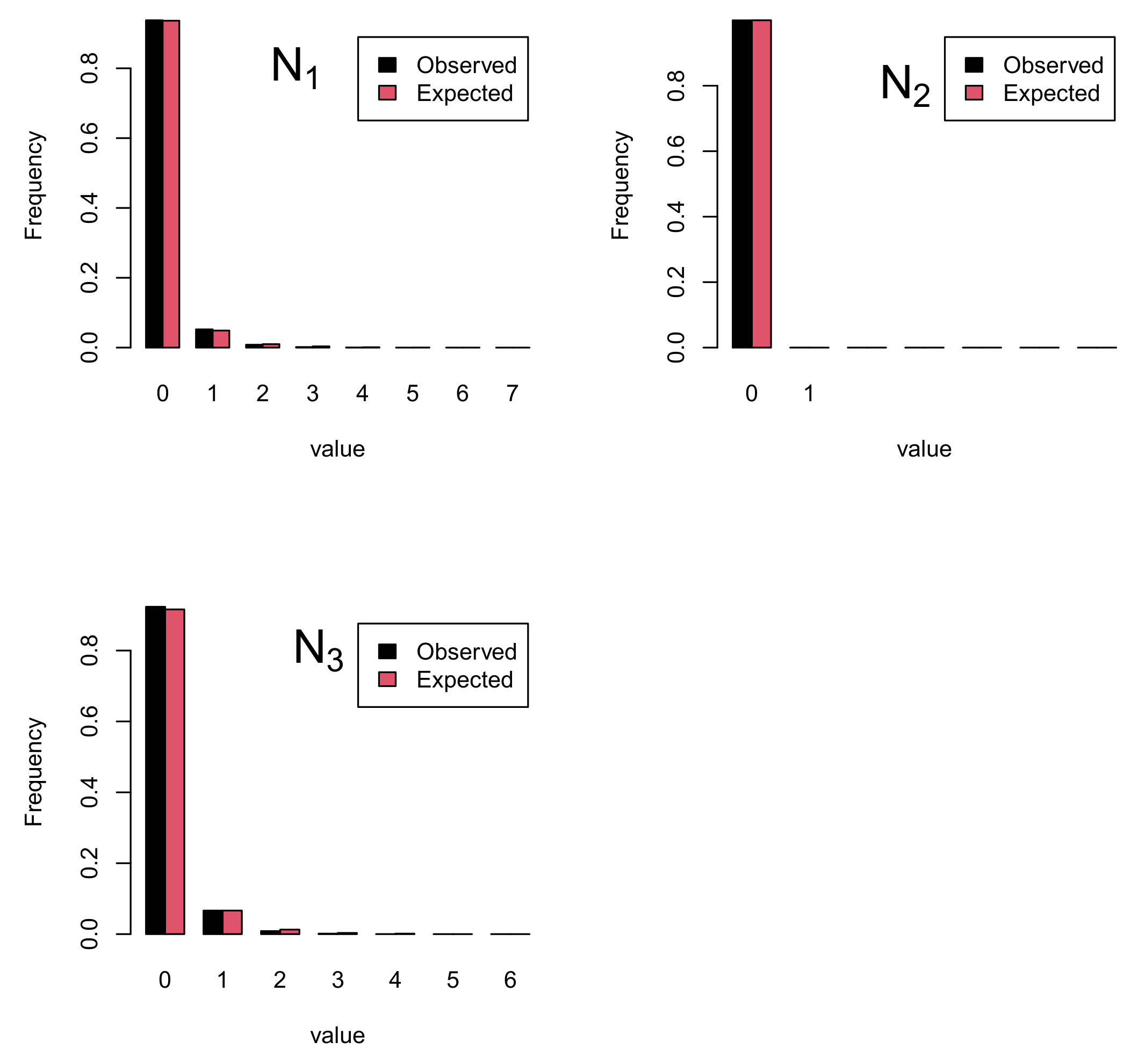
The marginal cases for the three variables can be seen in Figure 1. We have plotted for each of the three variables the observed and expected frequencies. Quite a good fit can be seen. Please note that for $N_2$, the observed values at $t=7$ had values of only 0 and 1. Overall, we believe that the model captures the underlying structure and describes the data at hand satisfactorily.

5. Conclusions

In this paper, we developed a model to account for time and cross dependence for a case of longitudinal multivariate count data. The time series part was captured by a MINAR model with a diagonal structure. This was sufficient to account for the time dependence in our case, but more complicated structure can be considered, such as a non-diagonal matrix $\mathbf{A}$ or higher order models. In addition, families like multivariate INGARCH models see [40] could be considered.

The dependence between the count variables was captured by Sarmanov-type multivariate distributions. This provides a flexible way to define multivariate distributions reducing computational needs, such as those that copula-based models have. In our case, we considered Poisson and negative binomial marginal distributions. Other choices like a zero-inflated model are also plausible, with small changes in the model development.

References

- Karlis, D. Models for multivariate count time series. In Handbook of Discrete-Valued Time Series; Chapman and Hall/CRC: Boca Raton, FL, USA, 2015; pp. 407–424. [Google Scholar]
- Bermúdez, L.; Guillén, M.; Karlis, D. Allowing for time and cross dependence assumptions between claim counts in ratemaking models. Insur. Math. Econ. 2018, 83, 161–1169. [Google Scholar] [CrossRef]
- Karlis, D.; Meligkotsidou, L. Multivariate Poisson regression with covariance structure. Stat. Comput. 2005, 15, 255–265. [Google Scholar] [CrossRef]
- Nikoloulopoulos, A.K. Copula-based models for multivariate discrete response data. In Copulae in Mathematical and Quantitative Finance; Springer: Berlin/Heidelberg, Germany, 2013; pp. 231–249. [Google Scholar]
- McKenzie, E. Some Simple Models for Discrete Variate Time Series. Water Resour. Bull. 1985, 21, 645–650. [Google Scholar] [CrossRef]
- Al-Osh, M.; Alzaid, A. First-Order Integer-Valued Autoregressive Process. J. Time Ser. Anal. 1987, 8, 261–275. [Google Scholar] [CrossRef]
- Steutel, F.; van Harn, K. Discrete Analogues of Self–Decomposability and Stability. Ann. Probab. 1979, 7, 893–899. [Google Scholar] [CrossRef]
- Franke, J.; Rao, T.S. Multivariate First-Order Integer-Valued Autoregressions; Technical Report; Forschung Universitat Kaiserslautern: Kaiserslautern, Germany, 1993. [Google Scholar]
- Latour, A. The multivariate GINAR(p) process. Adv. Appl. Probab. 1997, 29, 228–248. [Google Scholar] [CrossRef]
- Pedeli, X.; Karlis, D. Some properties of multivariate INAR(1) processes. Comput. Stat. Data Anal. 2013, 67, 213–225. [Google Scholar] [CrossRef]
- Pedeli, X.; Karlis, D. On composite likelihood estimation of a multivariate INAR(1) model. J. Time Ser. Anal. 2013, 34, 206–220. [Google Scholar] [CrossRef]
- Pedeli, X.; Karlis, D. An integer-valued time series model for multivariate surveillance. Stat. Med. 2020, 39, 940–954. [Google Scholar] [CrossRef] [PubMed] [Green Version]
- Sarmanov, O.V. Generalized normal correlation and two-dimensional Fréchet classes. In Doklady Akademii Nauk; Russian Academy of Sciences: Saint Petersburg, Russia, 1966; Volume 168, pp. 32–35. [Google Scholar]
- Ting Lee, M.L. Properties and applications of the Sarmanov family of bivariate distributions. Commun. Stat. Theory Methods 1996, 25, 1207–1222. [Google Scholar] [CrossRef]
- Lakshminarayana, J.; Pandit, S.; Srinivasa Rao, K. On a bivariate Poisson distribution. Commun. Stat. Theory Methods 1999, 28, 267–276. [Google Scholar] [CrossRef]
- Famoye, F. On the bivariate negative binomial regression model. J. Appl. Stat. 2010, 37, 969–981. [Google Scholar] [CrossRef]
- Famoye, F. A new bivariate generalized Poisson distribution. Stat. Neerl. 2010, 64, 112–124. [Google Scholar] [CrossRef]
- Hofer, V.; Leitner, J. A bivariate Sarmanov regression model for count data with generalised Poisson marginals. J. Appl. Stat. 2012, 39, 2599–2617. [Google Scholar] [CrossRef]
- Miravete, E.J. Multivariate Sarmanov Count Data Models; Discussion Paper No. DP7463; Centre for Economic Policy Research (CEPR): London, UK, 2009. [Google Scholar]
- Deshmukh, S.; Kasture, M. Bivariate distribution with truncated Poisson marginal distributions. Commun. Stat. Theory Methods 2002, 31, 527–534. [Google Scholar] [CrossRef]
- Famoye, F. Bivariate exponentiated-exponential geometric regression model. Stat. Neerl. 2019, 73, 434–450. [Google Scholar] [CrossRef]
- Krishna, P.M.; Tukaram, S.D. Bivariate zero-inflated power series distribution. Appl. Math. 2011, 2, 824. [Google Scholar] [CrossRef] [Green Version]
- Zhang, C.; Tian, G.; Huang, X. Two new bivariate zero-inflated generalized Poisson distributions with a flexible correlation structure. Stat. Optim. Inf. Comput. 2015, 3, 105–137. [Google Scholar] [CrossRef] [Green Version]
- Vernic, R. On a class of bivariate mixed Sarmanov distributions. Aust. N. Z. J. Stat. 2020, 62, 186–211. [Google Scholar] [CrossRef]
- Gomez-Deniz, E.; Sarabia, J.M.; Balakrishnan, N. A multivariate discrete Poisson-Lindley distribution: Extensions and actuarial applications. ASTIN Bull. J. IAA 2012, 42, 655–678. [Google Scholar]
- Zamani, H.; Faroughi, P.; Ismail, N. Bivariate Poisson-Lindley distribution with application. J. Math. Stat. 2015, 11, 1. [Google Scholar] [CrossRef] [Green Version]
- Cui, Y.; Zhu, F. A new bivariate integer-valued GARCH model allowing for negative cross-correlation. Test 2018, 27, 428–452. [Google Scholar] [CrossRef]
- Cui, Y.; Li, Q.; Zhu, F. Flexible bivariate Poisson integer-valued GARCH model. Ann. Inst. Stat. Math. 2019, 72, 1449–1477. [Google Scholar] [CrossRef]
- Buteikis, A.; Leipus, R. A copula-based bivariate integer-valued autoregressive process with application. Mod. Stoch. Theory Appl. 2019, 6, 227–249. [Google Scholar] [CrossRef]
- Khan, N.M.; Oncel Cekim, H.; Ozel, G. The family of the bivariate integer-valued autoregressive process (BINAR(1)) with Poisson–Lindley innovations. J. Stat. Comput. Simul. 2020, 90, 624–637. [Google Scholar] [CrossRef]
- Liu, F.; Pitt, D. Application of bivariate negative binomial regression model in analysing insurance count data. Ann. Actuar. Sci. 2017, 11, 390–411. [Google Scholar] [CrossRef] [Green Version]
- Bolancé, C.; Vernic, R. Multivariate count data generalized linear models: Three approaches based on the Sarmanov distribution. Insur. Math. Econ. 2019, 85, 89–103. [Google Scholar] [CrossRef] [Green Version]
- Rodríguez-Lallena, J.A.; Úbeda-Flores, M. Multivariate copulas with quadratic sections in one variable. Metrika 2010, 72, 331–349. [Google Scholar] [CrossRef]
- Famoye, F. A multivariate generalized Poisson regression model. Commun. Stat. Theory Methods 2015, 44, 497–511. [Google Scholar] [CrossRef]
- Vernic, R. On the evaluation of some multivariate compound distributions with Sarmanov’s counting distribution. Insur. Math. Econ. 2018, 79, 184–193. [Google Scholar] [CrossRef]
- Bermúdez, L. A priori ratemaking using bivariate Poisson regression models. Insur. Math. Econ. 2009, 44, 135–141. [Google Scholar] [CrossRef] [Green Version]
- Bermúdez, L.; Karlis, D. Bayesian multivariate Poisson models for insurance ratemaking. Insur. Math. Econ. 2011, 48, 226–236. [Google Scholar] [CrossRef] [Green Version]
- Bermúdez, L.; Karlis, D. A finite mixture of bivariate Poisson regression models with an application to insurance ratemaking. Comput. Stat. Data Anal. 2012, 56, 3988–3999. [Google Scholar] [CrossRef] [Green Version]
- Bermúdez, L.; Karlis, D. A posteriori ratemaking using bivariate Poisson models. Scand. Actuar. J. 2017, 2, 148–158. [Google Scholar] [CrossRef] [Green Version]
- Fokianos, K.; Støve, B.; Tjøstheim, D.; Doukhan, P. Multivariate count autoregression. Bernoulli 2020, 26, 471–499. [Google Scholar] [CrossRef] [Green Version]
Figure 1.
Observed and expected frequencies for time point for all individuals. Each plot corresponds to one of the three variables.