Improved Predictive Ability of KPLS Regression with Memetic Algorithms

Abstract

Kernel partial least squares regression (KPLS) is a non-linear method for predicting one or more dependent variables from a set of predictors, which transforms the original datasets into a feature space where it is possible to generate a linear model and extract orthogonal factors also called components. A difficulty in implementing KPLS regression is determining the number of components and the kernel function parameters that maximize its performance. In this work, a method is proposed to improve the predictive ability of the KPLS regression by means of memetic algorithms. A metaheuristic tuning procedure is carried out to select the number of components and the kernel function parameters that maximize the cumulative predictive squared correlation coefficient, an overall indicator of the predictive ability of KPLS. The proposed methodology led to estimate optimal parameters of the KPLS regression for the improvement of its predictive ability.

1. Introduction

The method of Partial least squares regression (PLS) has its origin in the field of economics with the work of Herman Wold [1] in the 1960s. It is currently popular in the social sciences, marketing and chemometrics [2]. PLS regression, however, is a linear method and is unsuitable to describe data structures that show variations with non-linear characteristics [3].

To solve the problem, Rosipal and Trejo [4] propose the Kernel partial least squares regression (KPLS) that transforms the original data sets into an arbitrary dimensionality feature space through non-linear mapping, and then creates a linear model in the feature space [5]. KPLS regression has been widely used in many scientific fields because of its high generalizability.

Shawe-Taylor and Cristianini [6] state that the improvement of classical multivariate statistical methods based on the decomposition into singular values with the use of kernel functions such as KPLS, is an area of research that has been widely used in recent years. Furthermore, Bennet and Embrechts [7] point out that future research should make full use of the potential of KPLS algorithms, that statistical learning theory can help clarify why KPLS generalizes well, and that implementing variants to KPLS could solve its limitations.

However, a recurrent problem is to determine the number of components (latent variables) and the parameters of the KPLS regression that maximize the predictive ability of the models generated [8]. Huang et al. [9] point out that the main problems in KPLS regression are the kernel function selection and the determination of its parameters, as well as the selection of the number of components; however, the selection of the kernel function remains an open problem. The usual choices of kernel functions found in the literature review are as follows [10,11]:

• Gaussian RBF kernel:

  $$k\left({\mathrm{x}}_i,{\mathrm{x}}_j\right)=\exp \left(-\sigma {∥{\mathrm{x}}_i-{\mathrm{x}}_j∥}^2\right)$$

  (1)
• Polynomial kernel:

  $$k\left({\mathrm{x}}_i,{\mathrm{x}}_j\right)={\left(\alpha \langle {\mathrm{x}}_i·{\mathrm{x}}_j\rangle +\beta \right)}^{\delta }$$

  (2)
• Hyperbolic tangent kernel:

  $$k\left({\mathrm{x}}_i,{\mathrm{x}}_j\right)=\tanh \left(\alpha \langle {\mathrm{x}}_i·{\mathrm{x}}_j\rangle +\beta \right)$$

  (3)

  where $\sigma$, $\alpha$, $\beta$ and $\delta$ are kernel parameters to be determined by various selection routes [10].

There is no theoretical basis for how to specify kernel function parameter values, however, they must be specified before any kernel-based method is performed. The most popular approach is to select them empirically and to a lesser extent cross-validation has been used to decide on kernel parameter values [10]. More recent studies have emphasised that kernel parameters must be optimised simultaneously with the selection of components, as these choices depend on each other [12,13].

The work of Fu et al. [13] presents a methodology for simultaneous estimation of the kernel function parameter and the number of components in KPCA and KPLS models. The aim of this paper is to propose a methodology to improve the predictive ability of the KPLS regression taking as reference the approach proposed by Mello-Román and Hernández [14,15] of metaheuristic tuning of the KPLS regression but using as iterative optimizer the Memetic algorithms (MA) in the selection of the number of components and the kernel function parameter.

Nature-inspired metaheuristic algorithms such as GA, PSO and others have demonstrated good performance in optimising KPLS regression, however, they require significant computational effort that increases significantly with increasing iterations [14,15]. In this article, MA is chosen as a KPLS regression optimizer because of its ability to generate optimal solutions in a reasonable time, even for very complex problem structures [16].

MA is considered a powerful problem solver in the field of continuous optimization, as it offers a balance between the exploration of the search space through its scheme of evolutionary algorithms and the focused exploitation of promising regions with a local search algorithm [16]. Algorithm design is not a trivial task and the non-existence of a universal optimiser suggests that algorithms designed efficiently must specifically address the characteristics of the problems to be optimised [17]. In this work, preliminary tests are carried out for the MA configuration, in order to determine the best balance between exploration and local search.

It is necessary to mention that there are other regression techniques used for predictive purposes such as Auto-Regressive Integrated Moving Average (ARIMA) [18] and others that have developed versions that introduce the kernel concept such as Support Vector Regression (SVR) and Gaussian Processes (GP) [19,20]. KPLS differs from them in that it addresses the problem of reducing the data dimensionality [10].

As for the robustness of kernel-based regression methods, some research has concluded that the choice of kernel function plays an important role in it [21,22]. A non-linear kernel function (for example, the Gaussian kernel function) leads to fairly robust regression methods with respect to outliers in the original input space. That is, non-linear modelling is not only attractive when the data structure is complex and a linear method may not be suitable, but can also be an interesting option when the data contain outliers [22].

2. Kernel Partial Least Squares Regression

Given an $X_{n\times m}$ array of independent variables ${\left\{x_i\right\}}_{i=1}^n\in {\mathbb{R}}^m$ and a $Y_{n\times r}$ array of response variables ${\left\{y_i\right\}}_{i=1}^n\in {\mathbb{R}}^r$.

Let us assume a non-linear transformation of the input variables ${\left\{x_i\right\}}_{i=1}^n$ in a feature space F provided with inner product; that is, $\mathsf{\phi }:x_i\in {\mathbb{R}}^m\to \mathsf{\phi }\left(x_i\right)\in F$. We denote by Φ a matrix (n × M) whose i-th row is the vector $\mathsf{\phi }\left(x_i\right)$. Depending on the non-linear transformation Φ(.) the feature space F can be highly dimensional.

The kernel function $k\left(x_i,x_j\right)=\mathsf{\phi }{\left(x_i\right)}^{\prime }·\mathsf{\phi }\left(x_j\right)$ calculates the inner product in the feature space F. The kernel matrix $K={\Phi \Phi }^{\prime }$ represents a matrix (n × n) of the cross products of the transformed data ${\left\{\mathsf{\phi }\left(x_i\right)\right\}}_{i=1}^n$, i.e., the element of the i-th row and the j-th column is the kernel matrix K is $k\left(x_i,x_j\right)$.

The KPLS regression algorithm proposed by Rosipal and Trejo [4] is as follows:

Algorithm 1. KPLS algorithm according to Rosipal and Trejo [4].

Start randomly u (any Y column) $t=Ku$, $t\leftarrow \frac{t}{∥t∥}$ $q=Y^{\prime }t$ $u=Yq$, u ← $\frac{u}{∥u∥}$‖ Repeat steps 2–5 until convergence Deflate K and Y matrices $K\leftarrow \left(I-t{t}^{\prime }\right)K\left(I-t{t}^{\prime }\right);Y\leftarrow \left(I-t{t}^{\prime }Y\right)$ where I is an n-dimensional identity matrix Repeat steps 2–7 until the U and T vectors have been removed

The deflation technique that is incorporated on step 6 of Algorithm 1 can be viewed as an implementation of Hotelling deflation [23,24]. After the extraction of the h components, with the generated matrices $T_{n\times h}$ and $U_{n\times h}$ the B matrix of coefficients of the KPLS regression is defined by the following expression:

$$\mathrm{B}={\mathsf{\Phi }}^{\prime }\mathrm{U}{\left({\mathrm{T}}^{\prime }\mathrm{KU}\right)}^{-1}{\mathrm{T}}^{\prime }\mathrm{Y}$$

(4)

Predictions on the training data set are obtained from the formula:

$$\widehat{\mathrm{Y}}=\mathrm{KU}{\left({\mathrm{T}}^{\prime }\mathrm{KU}\right)}^{-1}{\mathrm{T}}^{\prime }\mathrm{Y}={\mathrm{TT}}^{\prime }\mathrm{Y}$$

(5)

The expression is used for predictions in test data sets:

$${\widehat{\mathrm{Y}}}_t={\mathrm{K}}_t\mathrm{U}{\left({\mathrm{T}}^{\prime }\mathrm{KU}\right)}^{-1}{\mathrm{T}}^{\prime }\mathrm{Y}$$

(6)

where the $K_t$ matrix is the matrix $\left(n_t\times n\right)$ whose elements are the kernel functions $k_{ij}=k\left(x_i,x_j\right)$ evaluated on the values of the test set ${\left\{x_i\right\}}_{i=n+1}^{n+n_t}$ and the training set ${\left\{x_j\right\}}_{i=1}^n$ [3].

Before applying KPLS it is necessary to centralize the data in the feature space [25]. The following procedures can be applied for this purpose:

$$\mathrm{K}=\left(\mathrm{I}-\frac{1}{n}{1}_n{1_n}^{\prime }\right)\mathrm{K}\left(\mathrm{I}-\frac{1}{n}{1}_n{1_n}^{\prime }\right)$$

(7)

$${\mathrm{K}}_t=\left({\mathrm{K}}_t-\frac{1}{n}{1}_{n_t}{1_n}^{\prime }\mathrm{K}\right)\left(\mathrm{I}-\frac{1}{n}{1}_n{1_n}^{\prime }\right)$$

(8)

where I is again an n-dimensional identity matrix and $1_n$, $1_{n_t}$ represent the vectors whose elements are ones, with length n and $n_t$, respectively.

KPLS regression has over the years demonstrated high predictive performance; however, the choice of the optimal kernel function and its parameters is an open problem [7,26]. This research aims to contribute to the solution of the problem by applying an optimization algorithm. To do so, it is first necessary to define the mathematical function to be optimized.

Next, the mathematical structure of some indicators of the predictive ability of the KPLS regression is described.

Predictive Ability of KPLS

In any empirical modelling, it is essential to determine the correct complexity of the model. In the PLS/KPLS regression it is necessary to check the predictive significance of each component, and not to add up components that are not significant. According to Abdi [27], when the purpose of the regression is to generate models capable of predicting the value of the dependent variables in new observations, each component can only be considered relevant if it improves that prediction.

The cross-validation procedure is a practical and reliable way of testing predictive significance and has become the standard in PLS [28].

The cross-validation procedure is one of the oldest re-sampling techniques [29]. It consists of dividing the dataset into segments of size equal to k and then using k − 1 blocks to fit the model and validate it on the remaining segment. This procedure is done for all the k − 1 possible combinations of the k segments [30]. In this paper, the cross-validation procedure was applied to randomly divide the data set into k = 10 segments of equal size [31].

The way to evaluate the predictive ability of a model is by comparing the observed values and the predictions of the model [32]. Several studies take as an indicator the predictive ability in PLS/KPLS the root mean square error (RMSE) [13] or functions of it [33].

$$RMSE=\sqrt{\frac{PRESS}{n}}=\sqrt{\frac{{{\displaystyle \sum }}_1^n{\left({\widehat{y}}_i-{\mathrm{y}}_i\right)}^2}{n}}$$

(9)

where PRESS (Predictive Residual Sum of Squares) is the sum of the squared differences between the predictions ${\widehat{\mathbf{y}}}_i$ and the observed values $y_i$.

However, RMSE has the disadvantage that its values depend on the scales of measurements of the dependent variables, and in certain comparative studies it is not possible to use it. For this reason, the predictive ability of the models is often quantified in terms of the coefficient obtained from cross-validation processes, called by some authors the predictive squared correlation coefficient:

$$Q^2=1-\frac{{{\displaystyle \sum }}_1^n{\left({\widehat{y}}_i-{\mathrm{y}}_i\right)}^2}{{{\displaystyle \sum }}_1^n{\left({\mathrm{y}}_i-{\overline{\mathrm{y}}}_i\right)}^2}=1-\frac{PRESS}{RSS}$$

(10)

where RSS (Residual Sum of Square) is the sum of the squared differences of the observed values $y_{\mathrm{i}}$ with respect to the mean $\overline{y}$. In the PLS/KPLS regression, the coefficient $Q^2$ is calculated for each extracted component h. RSS is calculated using component h − 1 and PRESS using component h.

According to Thévenot [34], if the research interest is focused on evaluating the overall predictive ability of the PLS/KPLS regression model for a set of h > 1 components, a suitable indicator is the coefficient $Q_{cum}^2$, which evaluates the model’s capacity for generalization for a set of components {2, … h − 1, h}. It is obtained by means of the mathematical expression:

$$Q_{cum}^2=1-{\displaystyle \prod }_1^h\left(1-Q_h^2\right)$$

(11)

The coefficient $Q_{cum}^2$ takes values between 0 and 1, and the higher its value, the better the predictive performance [35].

As mentioned above, a key factor in PLS/KPLS regression is to define the optimal number of components. One criterion is to consider a significant component if ${\mathrm{Q}}^2\ge 0.0975$ or equivalent, to maintain the h component if $\sqrt{{\mathrm{PRESS}}_h}\le 0.95\sqrt{{\mathrm{RSS}}_{h-1}}$ [36].

Another criterion is to consider the optimal number of components according to the variation of the coefficients ${\mathrm{Q}}^2$ and ${\mathrm{Q}}_{\mathrm{cum}}^2$. The coefficient ${\mathrm{Q}}_{\mathrm{cum}}^2$ increases as components are added up to a certain maximum value and then decreases. Such critical point provides an estimate of the optimal number of components.

In this work the second approach is chosen: to evaluate the variation of the coefficient $Q_{cum}^2$ and to determine by optimal the number of components for which $Q_{cum}^2$ reaches its maximum value. This criterion is equivalent to considering a significant component if $\sqrt{{\mathrm{PRESS}}_h}\le \sqrt{{\mathrm{RSS}}_{h-1}}$ or $Q^2\ge 0$ [34].

3. Memetic Algorithms

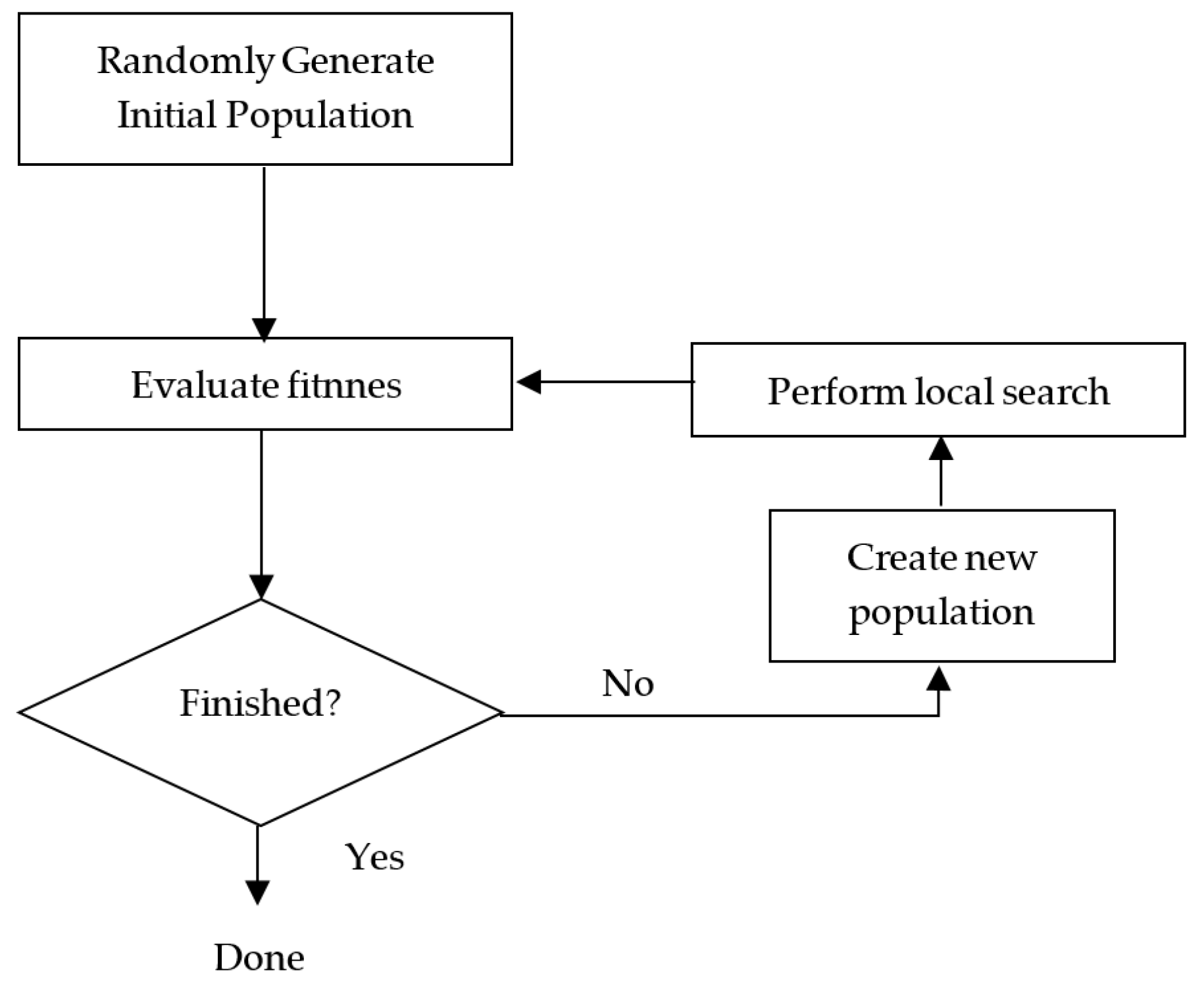
Moscato [37] introduces for the first time the term Memetic algorithms (MA) to refer to metaheuristic algorithms that show a hybrid approach. MA integrates evolutionary algorithms (such as GA) and a local search (LS) procedure to generate a hybrid algorithm with characteristics of both components. For a modern and detailed review, the text by Moscato and Cotta [38] can be used. Figure 1 shows a flowchart for a MA. At a simple level, the only difference between this and a flowchart for evolutionary algorithms is the extra “Perform local search” step [39].

Gogna and Tayal [40] describe the methodology used by MA in the following generic steps: MA starts with the generation of an initial population of solutions (individuals). This population can be generated randomly or, for better results, it can be generated using a heuristic (problem-specific) approach. The next step is the generation of a new population. This involves the use of several operations to generate offspring. The first operator is the selection operator which selects the best individual from the population in a similar way to that used in evolutionary algorithms. This is followed by the recombination of the selected individuals to produce offspring as in the case of GA. The generated offspring undergo mutations to increase the diversity of the population. The next step uses a local search operator to produce random variations in the generated population. This operation is repeated to search, in each individual’s environment, for a candidate solution that is better suited than the original solution.

MMA is conceived in an eclectic and pragmatic paradigm, open to the integration of other techniques (metaheuristic or not). Given the breadth of possibilities, it is worth noting that the algorithmic design used in this research is based on the proposal in [16]. The proposal implements MA variants with the paradigm of local search chains [41] which is denoted here MA-LS-Chains. Its main feature is the ability to apply LS several times in the same solution, using a fixed number of iterations/function evaluations each time. The final state of the LS parameters after each LS application becomes the initial point of a subsequent LS application on the same solution, creating an LS chain. MA-LS-Chains has proven to be more efficient than other algorithms, mainly in solving high-dimensional problems [16].

Algorithm 2 presents an example of a pseudocode for MA-LS-Chains. The Bergmeir et al. proposal [16] uses a steady-state genetic algorithm (SSGA) as evolutionary algorithm [42,43].

Algorithm 2. Pseudocode of MA-LS-Chains [16]

Generate the initial population   while not termination-condition do   Perform the SSGA with nfrec evaluations.   Build the set $S_{LS}$ of individuals which can be refined by LS.   Pick the best individual $c_{LS}$ in $S_{LS}$.   if $c_{LS}$ belongs to an existing LS chain then   Initialize the LS operator with the LS state stored with $c_{LS}$.   else   Initialize the LS operator with the default LS parameters.   end if   Apply the LS algorithm to $c_{LS}$ with $I_{str}$, giving crLS.   Replace $c_{LS}$ by crLS.   Store the final LS state with crLS. end while

After generating the initial population, the following steps are executed in a loop: the SSGA is run with a certain amount of evaluations nfrec. Then, the set $S_{LS}$ is built with the individuals of the population that have never been improved by the LS, or that have been improved by the LS but with an improvement (in fitness) superior to ${\delta }_{LS}^{\min }$, where ${\delta }_{LS}^{\min }$ is a parameter of the algorithm (by default ${\delta }_{LS}^{\min }={10}^{-8}$). If $\left|S_{LS}\right|\ne 0$, the LS is applied with an intensity of $I_{str}$ to the best individual in $S_{LS}$. If $S_{LS}$ is empty, the whole population is reinitialized except for the best individual which is maintained in the population [16].

4. Methodology

The main problems in KPLS are: the selection of the kernel function with its parameters and the number of components [9]. This research proposes a metaheuristic tuning procedure for the simultaneous estimation of the parameters of the kernel function and the number of components. It takes as objective function the coefficient $Q_{cum}^2$ and studies the performance of MA as optimization agent.

Given the original data matrices $X_{n\times m}$ and $Y_{n\times r}$, the kernel function $k\left(x_i,x_j\right)$ with parameter θ, and the kernel matrix $K_{n\times n}$ generated from $X_{n\times m}$ and $k\left(x_i,x_j\right)$. After performing the KPLS regression according to Algorithm 1 and extracting h components, the objective function is the coefficient $Q_{cum}^2\left(\theta ,h\right)$ determined by Equation (11), which is a function of the values that h and θ take in the KPLS regression. The optimization task can be written as follows:

$$(h,\theta )=\underset{h,\theta }{\mathrm{argmax}}{Q}_{cum}^2$$

(12)

$$\begin{gathered} \theta \in S\subset \mathbb{R} \\ h\in {\mathbb{Z}}^{+}\le m \end{gathered}$$

where the number of components h can take positive integer values lower than the number of columns in the $X$ matrix and the domain of the kernel function parameter θ is a predefined subset S of real numbers. The objective function $Q_{cum}^2$ is an indicator of the overall predictive power of the KPLS regression, it takes values between 0 and 1 and the higher its value, the higher the predictive power of the model [35]. It is obtained from cross-validation procedures and it is dimensionless, that is, it is not affected by the scales of the response variables.

To solve the optimization problem, an algorithm is implemented in a general iterative optimizer, in this case MA [15]. The problem is solved exclusively for feasible solutions of $\theta$ and $h$, infeasible solutions are discarded [44]. Algorithm 3 describes the steps of the proposed method:

Algorithm 3. KPLS parameters selection [15]

Given $X_{n\times m}$ the input matrix, $Y_{n\times r}$ the output matrix, a kernel function $k\left(x_i,x_j\right)$ with parameter $\theta \in S\subset \mathbb{R}$ The optimizer randomly generates an initial population p of θ (individuals). From $X_{n\times m}$ the input matrix, p kernel matrices $K_{n\times n}$ are generated, one matrix for each θ. KPLS regression (Algorithm 1) between $K_{n\times n}$ and $Y_{n\times r}$ is executed with $h\in {\mathbb{Z}}^{+}\le m$ components. $Q_{cum}^2$ is calculated by 10-fold cross-validation for each KPLS. Identify θ associated with the maximum $Q_{cum}^2$ and extract h for which this value is reached. g optimizer iterations are performed. The fitness function of the optimizer is max $Q_{cum}^2$. The optimizer determines the best values of θ and h and the optimal $Q_{cum}^2$.

The algorithm described in Algorithm 3 has a generic character. It is designed for population-based metaheuristic optimizers and can be used with different kernel functions. For this work, MA was used as the iterative optimizer and the Gaussian kernel function (Equation (1)), where the kernel function parameter $\theta =\sigma >0$.

Dataset and Pilot Framework

A data set on academic performance in Mathematics is used from individual characteristics of 899 Paraguayan students aged 12–15, from 16 educational institutions. The measurement instrument applied was a questionnaire to measure 9 predictor variables: Sex, Age, Classroom Learning, Bilingualism, Autonomous Learning, Academic Self-Concept, External Tutoring, Future Expectations and Work Status. Some of these predictor variables are multiple response. The response variable is the Mathematics academic performance of the participating students, determined on a numerical scale. The dataset is available in the GitHub digital repository at the following link: https://github.com/jorgemellopy/KPLS-MA (accessed on 25 February 2021).

In [45], this dataset was statistically modelled using Multiple Linear Regression (MLR). The value of the Coefficient of Determination obtained was R² = 37.9%, which represents the proportion of variability in academic performance that is attributed to the set of all predictor variables included in the model.

Preliminary tests are carried out for the MA configuration [46], to determine the best balance between exploration and intensification in the search space. This is done by taking different values of the parameter effort in MA. This parameter takes values between 0 and 1 giving the ratio of the number of evaluations performed in the local search and in the evolutionary algorithm (SSGA) [16].

The KPLS parameter selection algorithm (Algorithm 3) was run k = 30 times for each configuration [47], extracting the best results, mean and standard deviation of the estimates, and running time [48]. A non-parametric statistical analysis of the results obtained for the different MA configurations was carried out [49]. The Kruskal–Wallis test was used for independent samples, a non-parametric multiple comparison procedure. Kruskal–Wallis is an extension of the Mann–Whitney U test and is considered the non-parametric analogue of the one-way analysis of variance (ANOVA). Once an optimal configuration of the KPLS regression has been selected, the results obtained on the same dataset by other regression techniques such as MLR and PLS are compared.

All the experimental evaluations were carried out with the R software support. This required the installation of the following packages: plsdepot [50], kernlab [11], metaheuristicOpt [51] and Rmalschains [16]. The tests were performed simultaneously on a computer Intel^® Celeron^® CPUG1610 @ 2600 GHz, 4.00 GB RAM.

The package Rmalschains implements in its continuous optimization approach the following local search strategies [16]: Covariance Matrix Adaptation Evolution Strategy (CMAES) [52], Solis Wets solver (SW) [53], Subgrouping Solis Wets (SWW) [54] and Simplex [55]. The selection of the CMAES algorithm, in the continuous optimization approach, to perform the local search is due to the adaptability of its parameters, its fast convergence and it obtains very good results [16].

5. Results

5.1. Preliminary Tests

Preliminary tests were carried out to select the best value for the parameter effort in MA. This parameter constitutes the quotient between the number of evaluations made in the local search and the number of evaluations of SSGA. k = 30 runs of the proposed procedure (Algorithm 3) were performed for the values of effort = 0, 0.25, 0.50, 0.75 and 0.99. The population size of the evolutionary algorithm was set at p = 50, and the maximal number of evaluations of the fitness function was set at 5000.

In the k = 30 runs carried out, optimum values of $Q_{cum}^2$ have been reached more frequently with a number of components h = 2, for the different values of the parameter effort in MA. Values of h = 3 and h = 10 have also been obtained, although in a smaller proportion. The results are presented in

Table 1. Estimates of h for the values of the parameter effort in MA.

h	Effort
	0	0.25	0.50	0.75	0.99
2	27	28	28	28	30
3	2	2	2	2	0
10	1	0	0	0	0

.

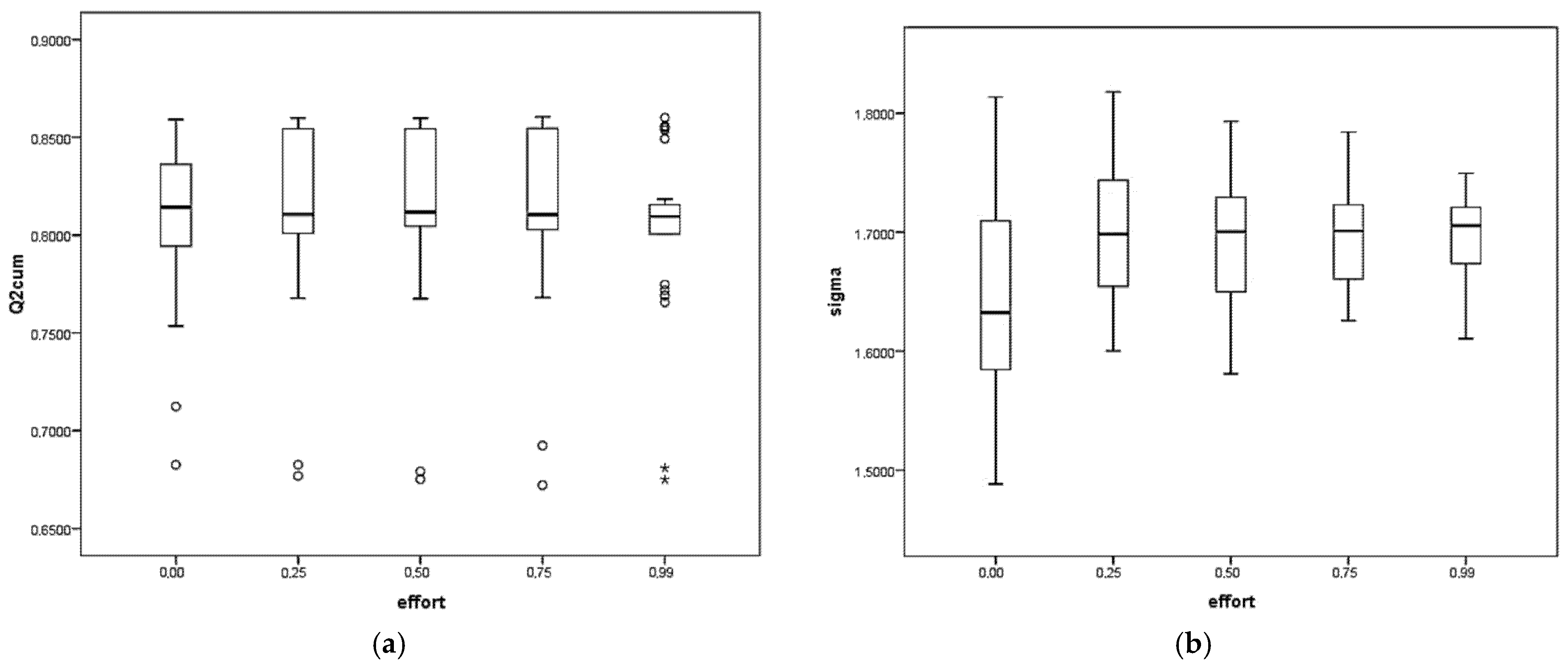
Taking only the estimates when the component number h = 2, the mean and standard deviation are extracted for the k = 30 runs made with each MA configuration. The estimates of $Q_{cum}^2$ and σ were very similar, with minimum variations observed in the dispersion with the increase of the value of the parameter effort. See Figure 2.

Table 2. Mean and standard deviation of $Q_{cum}^2$, $\sigma$ and running time estimates.

Algorithm	Effort	${\mathit{Q}}_{\mathit{c}\mathit{u}\mathit{m}}^2$		$\mathit{\sigma }$ Kernel Parameter		Running Time
		Mean	Std. Dev.	Mean	Std. Dev.	Mean	Std. Dev.
MA	0	0.8082	0.0432	1.6405	0.0902	6807.39	1286.97
	0.25	0.8087	0.0469	1.6993	0.0557	7406.65	586.91
	0.50	0.8098	0.0471	1.6900	0.0489	7487.20	802.50
	0.75	0.8101	0.0462	1.6964	0.0425	7452.20	692.13
	0.99	0.8032	0.0431	1.6960	0.0331	7369.65	543.85

shows the behavior of the estimates of $Q_{cum}^2$, $\sigma$ and running time for the different tested values of the parameter effort in MA. Minimal differences are observed in the running time, however, given the characteristics and conditions of the experiments they are not considered relevant. The longest running time obtained was 8281.5 s = 138 min.

The independent samples Kruskal–Wallis test was executed taking as null hypothesis the similarity of distributions of $Q_{cum}^2$, σ and the running time for the different values of the parameter effort in MA. The results presented in

Table 3. Independent-samples Kruskal–Wallis test summary.

Null Hypothesis	Sig.	Decision
The distribution of $Q_{cum}^2$ is the same across categories of effort	0.799	Retain the null hypothesis
The distribution of σ is the same across categories of effort	0.055	Retain the null hypothesis
The distribution of running time is the same across categories of effort	0.000 1	Reject the null hypothesis

¹ The significance level is 0.05.

indicate that there is no statistical evidence to reject the null hypothesis of similarity of distributions, both for the estimates of $Q_{cum}^2$ and σ. The dispersion in the running time leads to rejecting the null hypothesis at a significance level at α = 0.05.

Since there are no significant differences in the estimation of the kernel function parameter, the value of the parameter effort = 0.75 in MA is taken, for which the average estimation of $Q_{cum}^2$ is higher. Therefore, the KPLS regression is configured with a number of components h = 2 and σ = 1.6964.

In order to have a reference of the efficiency of MA in the proposed optimisation task, k = 30 runs of Algorithm 3 have been executed taking as optimisers: Genetic Algorithms (GA) and Particle Swarm Optimisation (PSO) [15], both with population size p = 50 and number of iterations equal to 20. The hyperparameters of these optimisers were determined at the default values set in the R packages used. GA and PSO also found maximum values of $Q_{cum}^2$ for h = 2, 28/30 and 26/30, respectively.

Table 4. Mean and standard deviation of $Q_{cum}^2$, $\sigma$ by MA, GA and PSO.

Algorithm	Hyperparameters	${\mathit{Q}}_{\mathit{c}\mathit{u}\mathit{m}}^2$		$\mathit{\sigma }$ Kernel Parameter
		Mean	Std. Dev.	Mean	Std. Dev.
MA	effort = 0.75 LS = CMAES	0.8101	0.0462	1.6964	0.0425
GA	crossover probability = 0.9 mutation probability = 0.1	0.7999	0.0368	1.5190	0.1258
PSO	maximum speed = 2 learning (c1, c2) = 1.49445	0.7934	0.0493	1.7035	0.0794

details the hyperparameters used and compares the results given by GA, PSO with MA, for h = 2.

Since the comparison of different metaheuristics as optimisers of the KPLS regression is not the main objective of this paper, no statistical analysis is included, however it is possible to observe that MA, GA and PSO obtain similar estimates of h, $\sigma$ and $Q_{cum}^2$.

5.2. Benchmarking Predictive Improvement

In [45], MLR was applied to the same dataset. The Determination coefficient obtained was R² = 37.9%, which represents the proportion of variability of the response variable explained by the set of six predictor variables included in the model, selected according to the reduction of the sum of squares of residuals resulting from including each predictor and the subsequent normalization of the values obtained, in a “Steps forward” selection process. The results obtained by the MLR are taken as a benchmark measure to evaluate the performance of the proposed method.

To evaluate the improvement in predictive ability in relation to simple PLS, the KPLS regression with Gaussian kernel function and parameter σ = 1.6964 was executed once again. The results for both methods with a number of components h = 2 are presented in

Table 5. Results of predictive ability of PLS and KPLS.

h	PLS			KPLS
	PRESS	${\mathit{Q}}^2$	${\mathit{Q}}_{\mathit{c}\mathit{u}\mathit{m}}^2$	PRESS	${\mathit{Q}}^2$	${\mathit{Q}}_{\mathit{c}\mathit{u}\mathit{m}}^2$
1	414.9032	0.260422158	0.2604222	556.393975	0.008210383	0.008210383
2	401.7303	−0.006134408	0.2558853	2.439731	0.683816165	0.686412155

.

The results allow us to identify an improvement in the predictive ability of the KPLS regression using the proposed methodology, taking as a reference both the results obtained by PLS in this trial and previous research on the same dataset. In general, the results are considered adequate in terms of the accuracy of the estimates and the computational effort required.

The proposed methodology for optimising the KPLS regression using MA has been implemented on other open datasets [56]. The results can be found in detail at [57], the conclusions are similar to those reached in this paper and lead to confirm the hypothesis of improving the predictive ability of KPLS by means of MA.

6. Discussion

This work addresses the problem of optimizing the predictive ability of the KPLS regression and proposes a metaheuristic tuning procedure for the selection of the parameters of the kernel function θ and the number of components h. The optimization problem is defined taking as an objective function the coefficient $Q_{cum}^2$, an indicator of the overall predictive ability of the KPLS regression obtained from cross-validation procedures. To solve the problem, a selection algorithm of the parameters θ and h is designed, incorporating a Memetic algorithm (MA) as an iterative optimizer.

Preliminary tests were carried out to obtain an adequate MA configuration and the right balance between exploration and local search. No significant differences were observed in the average estimates of $Q_{cum}^2$ and θ for different MA configurations. Through the proposed methodology, optimal values were selected for the kernel function parameter and the number of components in the KPLS regression. MA has performed well in terms of accuracy of estimates with a low running time.

The improved KPLS regression through the proposed procedure obtained better results than the PLS regression. The procedures described here may constitute a valid reference for the users of the technique who are looking for a better predictive performance. However, it is necessary to mention that the conclusions are limited to the evaluated dataset and the chosen computational tools.

Future research could study the effectiveness of the proposed method in mass data environments such as those frequently found in marketing, genomics, brain imaging, manufacturing and others. It is a natural extension of this research line, the search for an optimal configuration of the kernel function when it is integrated to other multivariate techniques.

References

- Wold, H. Soft Modelling by Latent Variables: The Non-Linear Iterative Partial Least Squares (NIPALS) Approach. J. Appl. Probab. 1975, 12, 117–142. [Google Scholar] [CrossRef]
- Pérez, R.A.; González-Farias, G. Partial least squares regression on symmetric positive-definite matrices. Rev. Colomb. Estad. 2013, 36, 177–192. [Google Scholar]
- Gao, Y.; Kong, X.; Hu, C.; Zhang, Z.; Li, H.; Hou, L. Multivariate data modeling using modified kernel partial least squares. Chem. Eng. Res. Des. 2015, 94, 466–474. [Google Scholar] [CrossRef]
- Rosipal, R.; Trejo, L.J. Kernel partial least squares regression in reproducing kernel hilbert space. J. Mach. Learn. Res. 2001, 2, 97–123. [Google Scholar]
- Zhang, H.; Liu, S.; Moraca, S.; Ojstersek, R. An Effective Use of Hybrid Metaheuristics Algorithm for Job Shop Scheduling Problem. Int. J. Simul. Model. 2016, 16, 644–657. [Google Scholar] [CrossRef]
- Shawe-Taylor, J.; Cristianini, N. Kernel Methods for Pattern Analysis; Cambridge University Press (CUP): Cambridge, UK, 2004. [Google Scholar]
- Bennett, K.P.; Embrechts, M.J. An optimization perspective on kernel partial least squares regression. In Advances in Learning Theory: Methods, Models and Applications; Nato Science Series sub series III computer and systems sciences; IOS Press: Amsterdam, The Netherlands, 2003; Volume 190, pp. 227–250. [Google Scholar]
- De Almeida, V.E.; Gomes, A.D.A.; Fernandes, D.D.D.S.; Goicoechea, H.C.; Galvão, R.K.H.; Araújo, M.C.U. Vis-NIR spectrometric determination of Brix and sucrose in sugar production samples using kernel partial least squares with interval selection based on the successive projections algorithm. Talanta 2018, 181, 38–43. [Google Scholar] [CrossRef]
- Huang, H.; Chen, B.; Liu, C. Safety Monitoring of a Super-High Dam Using Optimal Kernel Partial Least Squares. Math. Probl. Eng. 2015, 2015, 1–13. [Google Scholar] [CrossRef] [Green Version]
- Pilario, K.E.; Shafiee, M.; Cao, Y.; Lao, L.; Yang, S.-H. A Review of Kernel Methods for Feature Extraction in Nonlinear Process Monitoring. Processes 2019, 8, 24. [Google Scholar] [CrossRef] [Green Version]
- Karatzoglou, A.; Smola, A.; Hornik, K.; Zeileis, A. kernlab- AnS4Package for Kernel Methods inR. J. Stat. Softw. 2004, 11, 1–20. [Google Scholar] [CrossRef] [Green Version]
- Pilario, K.E.S.; Cao, Y.; Shafiee, M. Mixed kernel canonical variate dissimilarity analysis for incipient fault monitoring in nonlinear dynamic processes. Comput. Chem. Eng. 2019, 123, 143–154. [Google Scholar] [CrossRef] [Green Version]
- Fu, Y.; Kruger, U.; Li, Z.; Xie, L.; Thompson, J.; Rooney, D.; Hahn, J.; Yang, H. Cross-validatory framework for optimal parameter estimation of KPCA and KPLS models. Chemom. Intell. Lab. Syst. 2017, 167, 196–207. [Google Scholar] [CrossRef] [Green Version]
- Mello-Román, J.D.; Hernandez, A. KPLS optimization approach using genetic algorithms. Procedia Comput. Sci. 2020, 170, 1153–1160. [Google Scholar] [CrossRef]
- Mello-Roman, J.D.; Hernandez, A. KPLS Optimization with Nature-Inspired Metaheuristic Algorithms. IEEE Access 2020, 8, 157482–157492. [Google Scholar] [CrossRef]
- Bergmeir, C.; Molina, D.; Benıtez, J.M. Memetic Algorithms with Local Search Chains in R: The Rmalschains Package. J. Stat. Softw. 2016, 75, 1–33. [Google Scholar] [CrossRef]
- Caraffini, F.; Neri, F.; Epitropakis, M. HyperSPAM: A study on hyper-heuristic coordination strategies in the continuous domain. Inf. Sci. 2019, 477, 186–202. [Google Scholar] [CrossRef]
- Thiyagarajan, K.; Kodagoda, S.; Ranasinghe, R.; Vitanage, D.; Iori, G. Robust sensor suite combined with predictive analytics enabled anomaly detection model for smart monitoring of concrete sewer pipe surface moisture conditions. IEEE Sens. J. 2020, 20, 8232–8243. [Google Scholar] [CrossRef]
- Rasmussen, C.E. Gaussian processes in machine learning. In Summer School on Machine Learning; Springer: Berlin/Heidelberg, Germany, 2003; pp. 63–71. [Google Scholar]
- Thiyagarajan, K.; Kodagoda, S.; Ulapane, N. Data-driven machine learning approach for predicting volumetric moisture content of concrete using resistance sensor measurements. In Proceedings of the 2016 IEEE 11th Conference on Industrial Electronics and Applications (ICIEA), Hefei, China, 5–7 June 2016; pp. 1288–1293. [Google Scholar]
- Christmann, A.; Steinwart, I. Consistency and robustness of kernel based regression. In Technical Report; SFB-475; University of Dortmund: Dortmund, Germany, 2005. [Google Scholar]
- Rousseeuw, P.J.; Debruyne, M.; Engelen, S.; Hubert, M. Robustness and Outlier Detection in Chemometrics. Crit. Rev. Anal. Chem. 2006, 36, 221–242. [Google Scholar] [CrossRef]
- Lewi, P.J. Pattern recognition, reflections from a chemometric point of view. Chemom. Intell. Lab. Syst. 1995, 28, 23–33. [Google Scholar] [CrossRef]
- Hotelling, H. Analysis of a complex of statistical variables into principal components. J. Educ. Psychol. 1933, 24, 417. [Google Scholar] [CrossRef]
- Schölkopf, B.; Smola, A.; Müller, K.-R. Nonlinear Component Analysis as a Kernel Eigenvalue Problem. Neural Comput. 1998, 10, 1299–1319. [Google Scholar] [CrossRef] [Green Version]
- Rivas, J.A.M.; Cerrillo, S.F.J. Un algoritmo genético para selección de kernel en Análisis de Componentes Principales con Kernels. Investig. Oper. 2014, 35, 148–157. [Google Scholar]
- Abdi, H. Partial least squares regression and projection on latent structure regression (PLS Regression). Wiley Interdiscip. Rev. Comput. Stat. 2009, 2, 97–106. [Google Scholar] [CrossRef]
- Wold, S.; Sjöström, M.; Eriksson, L. PLS-regression: A basic tool of chemometrics. Chemom. Intell. Lab. Syst. 2001, 58, 109–130. [Google Scholar] [CrossRef]
- Stone, M. Cross-Validatory Choice and Assessment of Statistical Predictions. J. R. Stat. Soc. Ser. B (Stat. Methodol.) 1974, 36, 111–133. [Google Scholar] [CrossRef]
- Bischl, B.; Mersmann, O.; Trautmann, H.; Weihs, C. Resampling Methods for Meta-Model Validation with Recommendations for Evolutionary Computation. Evol. Comput. 2012, 20, 249–275. [Google Scholar] [CrossRef]
- Xue, S.; Yan, X. A new kernel function of support vector regression combined with probability distribution and its application in chemometrics and the QSAR modeling. Chemom. Intell. Lab. Syst. 2017, 167, 96–101. [Google Scholar] [CrossRef]
- Consonni, V.; Ballabio, D.; Todeschini, R. Evaluation of model predictive ability by external validation techniques. J. Chemom. 2010, 24, 194–201. [Google Scholar] [CrossRef]
- Jalali-Heravi, M.; Kyani, A. Application of genetic algorithm-kernel partial least square as a novel nonlinear feature selec-tion method: Activity of carbonic anhydrase II inhibitors. Eur. J. Med. Chem. 2007, 42, 649–659. [Google Scholar] [CrossRef]
- Thévenot, E.A. Ropls: PCA, PLS (-DA) and OPLS (-DA) for Multivariate Analysis and Feature Selection of Omics Data. 2020. Available online: https://master.bioconductor.org/packages/release/bioc/vignettes/ropls/inst/doc/ropls-vignette.html (accessed on 27 October 2020).
- Eriksson, L.; Johansson, E.; Antti, H.; Holmes, E. Multi-and megavariate data analysis. In Metabonomics Toxicity Assessment; CRC Press: Boca Raton, FL, USA, 2005; pp. 263–336. [Google Scholar]
- Binard, C. Introduction à la Regression PLS (Groupe de Travail PLS). 2012. Available online: https://docplayer.fr/42840787-Introduction-a-la-regression-pls-carole-binard.html (accessed on 27 October 2020).
- Moscato, P. On evolution, search, optimization, genetic algorithms and martial arts: Towards memetic algorithms. In Caltech Concurrent Computation Program, C3P Report; California Institute of Technology: Pasadena, CA, USA, 1989; Volume 826. [Google Scholar]
- Moscato, P.; Cotta, C. A Modern Introduction to Memetic Algorithms. In International Series in Operations Research & Management Science; Springer International Publishing: Berlin, Germany, 2010; Volume 146, pp. 141–183. [Google Scholar]
- Ryan, C. Evolutionary Algorithms and Metaheuristics. In Encyclopedia of Physical Science and Technology, 3rd ed.; Meyers, R.A., Ed.; Elsevier: Amsterdam, The Netherlands, 2001; pp. 673–685. [Google Scholar]
- Gogna, A.; Tayal, A. Metaheuristics: Review and application. J. Exp. Theor. Artif. Intell. 2013, 25, 503–526. [Google Scholar] [CrossRef]
- Molina, D.; Lozano, M.; García-Martínez, C.; Herrera, F. Memetic Algorithms for Continuous Optimisation Based on Local Search Chains. Evol. Comput. 2010, 18, 27–63. [Google Scholar] [CrossRef]
- Whitley, D. The GENITOR Algorithm and Selection Pressure: Why Rank-Based Allocation of Reproductive Trials Is Best. In Proceedings of the Third International Conference on Genetic Algorithms, San Francisco, CA, USA, December 1989; pp. 116–121. [Google Scholar]
- Smith, J.E. Genetic Algorithms. In Handbook of Global Optimization, Volume 62 of Nonconvex Optimization and Its Applications; Pardalos, P.M., Romeijn, H.E., Eds.; Springer: Berlin/Heidelberg, Germany, 2002; pp. 275–362. [Google Scholar]
- Caraffini, F.; Kononova, A.V.; Corne, D. Infeasibility and structural bias in differential evolution. Inf. Sci. 2019, 496, 161–179. [Google Scholar] [CrossRef] [Green Version]
- Mello Román, J.D.; Hernández Estrada, A. Un estudio sobre el rendimiento académico en Matemáticas. Rev. Electrón. Investig. Educ. 2019, 21, 1–10. [Google Scholar] [CrossRef]
- Carrero Yubero, C. Análisis de Técnicas Evolutivas para la Estimación de Curvas de Tipos de Interés. Master’s Thesis, Universidad Carlos III de Madrid, Getafe, Spain, 2011. [Google Scholar]
- Vidal, P.J.; Olivera, A.C. DNA fragment assembling using a novel GPU firefly algorithm. Dyna 2018, 85, 108–116. [Google Scholar] [CrossRef]
- Osaba, E.; Carballedo, R.; Diaz, F.; Onieva, E.; Masegosa, A.; Perallos, A. Good practice proposal for the implementation, presentation, and comparison of metaheuristics for solving routing problems. Neurocomputing 2018, 271, 2–8. [Google Scholar] [CrossRef] [Green Version]
- Derrac, J.; García, S.; Molina, D.; Herrera, F. A practical tutorial on the use of nonparametric statistical tests as a methodol-ogy for comparing evolutionary and swarm intelligence algorithms. Swarm Evolut. Comput. 2011, 1, 3–18. [Google Scholar] [CrossRef]
- Sanchez, G. plsdepot: Partial least squares (PLS) data analysis methods. In R Package Version 0.1, 17; R Core Team: Vienna, Austria, 2012. [Google Scholar]
- Riza, L.S.; Nugroho, E.P. MetaheuristicOpt: An R Package for Optimisation Based on Meta-Heuristics Algorithms. Pertanika J. Sci. Technol. 2018, 26, 1401–1412. [Google Scholar]
- Hansen, N.; Müller, S.D.; Koumoutsakos, P. Reducing the Time Complexity of the Derandomized Evolution Strategy with Covariance Matrix Adaptation (CMA-ES). Evol. Comput. 2003, 11, 1–18. [Google Scholar] [CrossRef]
- Solis, F.J.; Wets, R.J.-B. Minimization by Random Search Techniques. Math. Oper. Res. 1981, 6, 19–30. [Google Scholar] [CrossRef]
- Molina, D.; Lozano, M.; Sánchez, A.M.; Herrera, F. Memetic algorithms based on local search chains for large scale continuous optimisation problems: MA-SSW-Chains. Soft Comput. 2010, 15, 2201–2220. [Google Scholar] [CrossRef]
- Nelder, J.A.; Mead, R. A Simplex Method for Function Minimization. Comput. J. 1965, 7, 308–313. [Google Scholar] [CrossRef]
- Dua, D.; Graff, C. UCI Machine Learning Repository; University of California, School of Information and Computer Science: Irvine, CA, USA, 2019. [Google Scholar]
- Mello-Román, J.D. Optimización de la Regresión de Mínimos Cuadrados Parciales con Funciones Kernel. Ph.D. Thesis, Universidad Complutense de Madrid, Madrid, Spain, 2021. [Google Scholar]
Figure 1.
Flowchart for a simple MA [39].
Figure 2.
(a) Estimates of for different values of the parameter effort; (b) Estimates of for different values of the parameter effort.