Modeling the Effect of Different Forest Types on Water Balance in the Three Gorges Reservoir Area in China, with CoupModel

Abstract

Precipitation, throughfall, stemflow, and soil water content were measured, whereas interception, transpiration, evaporation, deep percolation, and soil water recharge were estimated in three plots, including oak (Lithocarpus glaber), Chinese fir (Cunninghamia lanceolata) forestlands, and maize (Zea mays) farmland in the Three Gorges Reservoir in China. A physical process-based model (CoupModel) was set up with climatic measurements as input and was calibrated with throughfall and vertical frequency domain reflectometry measurements from January 2018 to December 2019. Simulated values of soil moisture were fairly consistent with measured ones, with a determination coefficient (R²) of 0.73–0.91. Evapotranspiration was the main output of water balance, with a percentage of up to 61%, and such output was ranked as follows: oak forest (720 mm/y) > Chinese fir forest (700 mm/y) > maize farmland (600 mm/y). Afforestation influenced water balance, and water recharge was generally less significant in oak forestland than in Chinese fir forestland. Annual simulated deep percolation decreased by 60 mm for oak and 47 mm for Chinese fir compared with that for farmland (452 mm/y) and even more significantly in wet years. This decrease was mainly attributed to increased interception (122–159 mm/y) and transpiration (49–84 mm/y) after afforestation. Simulations indicated that vegetation species significantly influenced the magnitude of water balance components, calling for further attention to the selection of regrown tree species in the planning for afforestation projects, particularly for such projects that aim to improve the quantity of water infiltrating groundwater. Soil and water conservation measures should also be applied scientifically when converting farmland to forest in this area, particularly in the oak forest stand.

1. Introduction

The Three Gorges Dam is the largest hydroelectric scheme in the world. With the construction of this huge project, human interference and destruction inevitably impacted the natural ecosystem of the Three Gorges Reservoir area (TGRA). The expansion of the reservoir inundation area and the implementation of the migration project will significantly influence the ecological environment, including plants, wild animals, forest soil, and air quality in TGRA [1,2,3]. TGRA is a typical case in terms of the complexity of the natural environment and the fragility of ecosystems in China [4,5]. In the late 1980s, the forest coverage rate was only 19.9%, even less than 5% at a few sections, and soil was severely eroded in this region. Thus, vegetation recovery was of great significance to the ecological environment construction and economic sustainable development of TGRA. The Chinese central government enacted a series of policies since 1989, such as the Natural Forest Protection Project and the Shelter–Forest Construction Project in the upstream and midstream of the Yangtze River; much effort was made on vegetation restoration to reduce soil and water loss, improve coverage rate, and protect the water source of the area [3]. Given these policies, much of the inefficiently cultivated land (especially slope lands) was converted to forest in this region. By 2000, afforested areas had reached 6.74 million hm², the forest coverage rate had changed to 25%, and the soil erosion area had been reduced by 42% [3,5].

Trees considerably affect runoff via such features as albedo [6], stomatal behavior or transpiration [7], root growth [8], and leaf area [9]. The conversion of arable land to forest may significantly decrease runoff by increasing evapotranspiration, whereas deforestation usually enhances runoff [10]. In wet temperate climates, the substantial use of water by trees is mainly due to the interception of rainfall by their rough canopies [7,11,12,13] and soil water consumption by their deeper roots [8] than those of short cropland vegetation. Although large variability exists because of differences in climate, soil, and vegetation, analyses of the effect of afforestation or deforestation on water recharge indicate that a shift from low vegetation, such as arable crop or grassland, to mature forest reduces water recharge by 25% to 45% [14,15]. In China, Sun [16] suggests that the average water yield reduction may vary from about 50 mm/y (50%) in the semi-arid Loess Plateau in northern China to about 300 mm/y (30%) in the tropical southern region. Moreover, water balance can be influenced by different vegetation types. Bosch and Hewlett [17] proposed that for every 10% increase in forest cover, annual water yield decreases by 40 mm/y in coniferous forest, and by 25 and 10 mm/y in deciduous broadleaved forest and shrubbery. Stecdnick [18] obtained similar results from experiments on 95 catchments in the U.S. Van der Salm [19] found that water recharge is generally less significant in coniferous/Norway spruce forest (100–191 mm/y) than in deciduous/common oak forest (149–192 mm/y). Other important factors that influence water balance include site conditions (e.g., slope), afforestation management (e.g., stand age, planting density, thinning, and forest structure), soil conditions (e.g., texture, organic matter content, and hydraulic characteristics) [10,12,20,21]. Most studies on TGRA have focused on the benefits of forests in reducing large floods and soil erosion or on single processes, such as evapotranspiration, soil water changes, and infiltration processes for different species [4,5,21,22], but analyses of water balance components within soil–vegetation–atmosphere transfer (SVAT) systems and water recharge after afforestation are scarce.

Traditionally, the components of evapotranspiration, soil evaporation, and transpiration are technically complicated and are associated with uncertainty in measurement procedure under field conditions [23]. One way to quantify the constituents of water balance in forest ecosystems is to use water balance models based on soil, vegetation, and atmosphere characteristics (SVAT models). The CoupModel is a well-established SVAT model [24] that has been revised several times [25]. Ladekarl [26], Christiansen [27], and Schmidt-Walter and Lamersdorf [28] all used CoupModel to calculate water balance among different ecosystems. In China, applications of CoupModel have mainly concentrated in the northern area. For example, Zhang [23] used CoupModel to assess the effects of wheat straw mulch and fallow crops on water balance and water use efficiency in the Loess Plateau. Wang [12] investigated two types of planted vegetation (Liaodong oak and black locust forest), modeled water transfer with CoupModel, and explored the importance of vegetation type in relation to water balance in the hill and gully region of the Loess Plateau. Wu [29] and Zhou [30] explored the hydrological processes of frozen soil in the northeast China and Tibetan Plateau through CoupModel. However, CoupModel has rarely been applied in TGRA.

As a part of vegetation restoration projects, we conducted this research to determine the difference in water balance components among vegetation patterns and to assess changes in water balance and water consumption after the afforestation of arable land. From January 2018 to December 2019, we measured precipitation, throughfall, stemflow, and soil water content in three plots, including oak (Lithocarpus glaber) forest, Chinese fir (Cunninghamia lanceolata) forest, and maize (Zea mays) farmland, and calculated hydrological fluxes in TGRA through CoupModel.

2. Materials and Methods

2.1. Site Description

The study site is located in the middle part of Simian Mountain in southwestern China (28°31′–28°46′ N, 106°17′–106°30′ E), upstream of the Yangtze River. This region is also at the upper end of TGRA, a typical case in terms of the complexity of the natural environment and the fragility of ecosystems in China [4,5].

Simian Mountain is located in a subtropical area and has a continental monsoon climate, with plenty of precipitation. The elevation ranges from 900 m to 1500 m above sea level. The mean annual air temperature was 18.4 °C, varying seasonally from approximately −5.5 °C in January to more than 31.5 °C in August [5]. The mean annual precipitation was 1096.7 mm (1951–2019) and was normally concentrated from May to September. The experiment was carried out from January 2018 to December 2019.

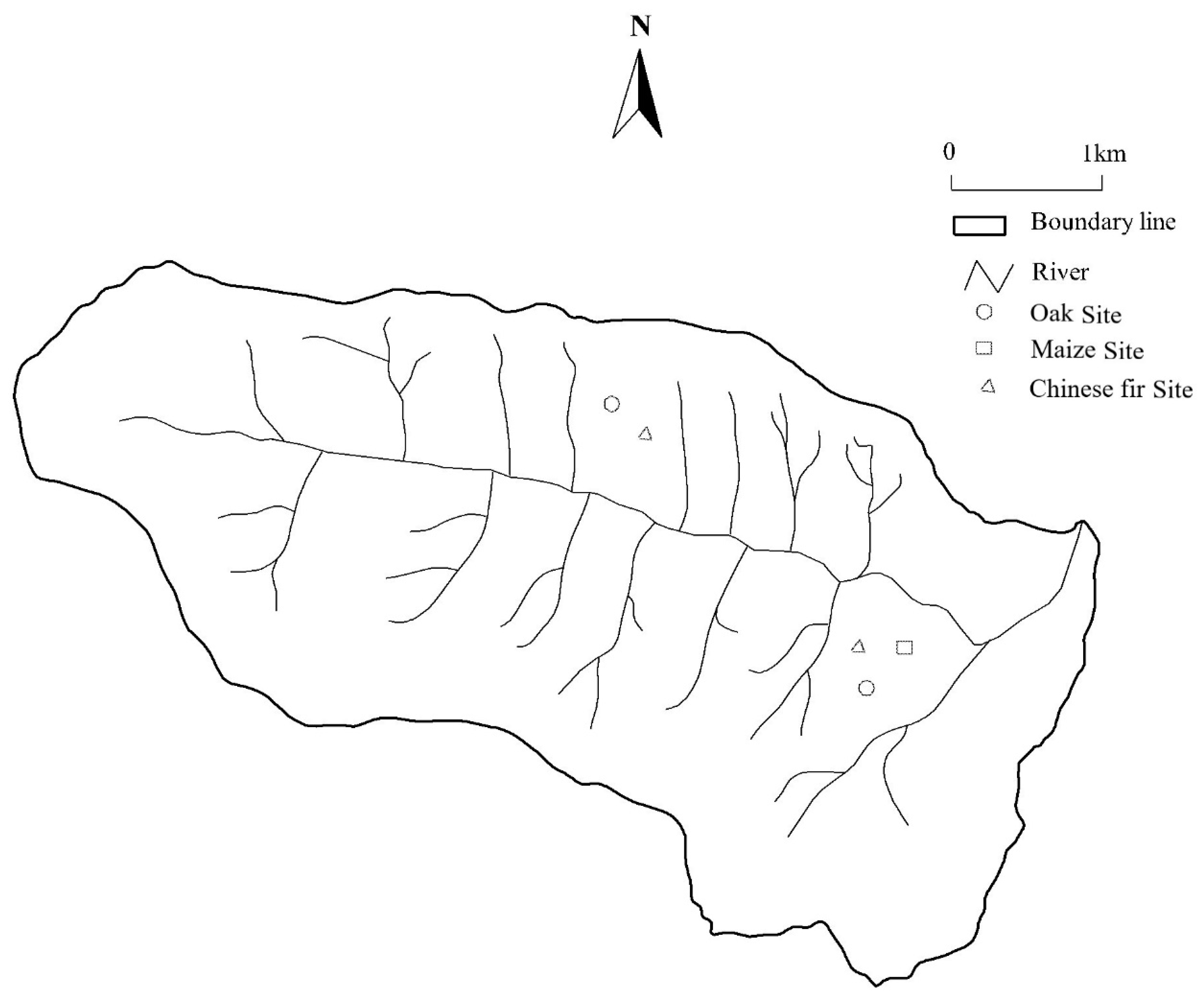
Two forests plots (oak and Chinese fir) and one farmland plot (maize) were investigated in the Shuangqiaoxi and Qinjiagou watersheds, respectively. Figure 1 shows the plot distribution. The first forest stand comprised oak (Lithocarpus glaber) with an average tree height of 12 m and a mean stem diameter at breast height of 14 cm (in 2018). The second forest stand comprised Chinese fir (Cunninghamia. lanceolata), with an average tree height of 14 m and a mean stem diameter at breast height of 10.2 cm (in 2018). These stands were planted in the 1980s to form shelter woods to control soil and water loss. Stand density was approximately 1000 trees/ha. The third plot, located on conventionally managed farmland, was planted with maize (Zea mays) from May to September. The two forest stands were converted from arable land many years before the experiments. During the experimental period, all plots received no fertilization or irrigation, and no natural compensation of groundwater resources was observed because of the deep water table. According to the international texture classification system, the three plots displayed similar soil textural characteristics (i.e., sandy loam). Basic information on the experimental plots is presented in

Table 1. Basic information on standard land of experimental plots.

Vegetation Type	Elevation	Gradient	Aspect	Age of Trees	Canopy Height	Tree DBH 1	Density	Coverage	Main Vegetation
	/m	/(°)	-	-	/m	/cm	/(Plant·ha−1)	/%	-
Oak	1167	5	SW	20	12.0	14	1000	90	Lithocarpus glaber, Schima superba gardn champ, Hicriopteris chinensis, Pteridium aquilinum
Chinese fir	1178	6	SW	20	14.0	10.2	1000	75	Cunninghamia lanceolata, Pinus massoniana Lespedeza bicolor, Aster ageratoides
Maize	1165	3	SW	-	1.2	-	-	85	Zea mays

¹ DBH is diameter at breast height.

.

2.2. Field Data

2.2.1. Meteorological Variables

Hourly meteorological data, including precipitation, global radiation, air temperature, wind speed, and relative humidity, were recorded by an automatic weather station Vantage PRO2 (Davis Instruments Corp., Hayward, CA, USA) positioned at a clear-cut area 600 m from the farmland experimental field. Measurements were taken at a height of 2 m. Sensors were factory-calibrated before installation.

2.2.2. Measurement of Soil Moisture Content

Soil volumetric water content (θ) was measured by frequency domain reflectometry (FDR; Diviner 2000, Adelaide, Australia). Before the experiment, nine PVC probes (three samples in each plot) were vertically installed in mineral soil after the removal of the O-horizon (if present). Daily readings of soil moisture content (SMC) were recorded at 10 cm depth intervals from the surface down to 80 cm from 1 January 2018 to 31 December 2019. The FDR sensors were calibrated in the field by the comparison of measured soil water gravimetric content in all replicate plots during the experimental period.

2.2.3. Throughfall and Stemflow Measurement

Throughfall (TF) was collected in three plastic buckets beneath three standard trees in forest stands with an area of 314 cm², and water was gathered in measuring cylinders after rainfall. Filters were placed over the top of the containers to avoid contamination of the sample by leaves and animals [27]. Stemflow (SF) was collected through a longitudinally split PVC tube around the trunks of three separate trees at a 1.5 m height in each stand and sealed with silicone along the trunk to avoid water running beneath the tube. The tube bottom was connected to a closed bucket on the ground [12,13,27]. After the rainfall, canopy interception capacity was calculated by precipitation (P) minus TF and SF.

2.2.4. Vegetation Properties

Vegetation characteristics, such as leaf area index (LAI), canopy height, and vertical root distributions, were surveyed for use as model input. LAI was measured with a LAI-2000 Plant Canopy Analyzer (LICOR, Lincoln, USA) once a month in the growing seasons of 2018 and 2019, with at least 10 adjacent plants on each occasion. In the three plots, 10 plants were chosen as standards, and their heights were surveyed with a measuring rod once a month during growing season [12,13]. Root depth was investigated by excavating the soil profile, and this procedure was repeated once a month in growing seasons.

2.2.5. Collection of Soil Samples and Laboratory Analyses

Volume-intact soil samples were taken through steel cylinders (100 cm³) [27] at 10 cm depth intervals to a depth of 80 cm in April 2018. Within each horizon, three replicates were taken to eliminate soil heterogeneity. The soil samples were kept cold and dark until analyzed.

Soil physical characteristics were determined in the laboratory. The particle size of the soil samples was analyzed by the hydrometer method 4, and saturated hydraulic conductivity (mm/d) was measured by the constant hydraulic head method [12,13]. In addition, parameters in the Brooks–Corey equation [31] were estimated according to measured points of pF curves by a pressure membrane apparatus (1500F1, Soil Moisture Corp., USA). Soil parameter values in CoupModel were mainly derived from measurements in laboratory, but they also required calibration during simulation.

2.2.6. Surface Runoff

Runoff plots were established to measure surface runoff beside every stand. The size of each runoff plot was 5 m × 20 m. At the bottom of the runoff plots, iron runoff buckets were installed to collect runoff. The size of the runoff buckets, 80 cm in diameter and 100 cm in height, was designed according to the hydrological data derived from the Jiangjin meteorological station. After each runoff event, the water level in the runoff buckets was measured to calculate runoff volume [1313]. Given that the topography was flat, no surface runoff was found during the experimental period.

2.3. Model Description

CoupModel 3.0 is a one-dimensional (1D) model that simulates fluxes of water, heat, carbon, and nitrogen in the soil–plant–atmosphere system, combining the SOIL and SOILN models [24,25]. This model is a complex model that simulates water and heat processes in soil on the basis of well-known physical equations. Two coupled differential equations for water and heat flow represent the core of the model. A detailed technical description of the model was given by Jansson and Karlberg [24].

Water balance over a period of time can be expressed as follows:

$$P=I+E_t+E_s+D+\Delta S+R+TR$$

(1)

where P is precipitation, I is interception, Et is plant transpiration, Es is soil evaporation, D is deep percolation, ΔS is the change in soil water storage, R is surface runoff, TR represents man made alterations of the water balance, here it is zero because no system was modified externally by human intervention.

Soil water flow is the sum of matrix, vapor, and bypass flow and is assumed to obey Darcy’s law as generalized for unsaturated flow by Richards [32]. Soil texture and water retention curves are used as model inputs, whereas the Brooks–Corey equation [32] in combination with the Mualem equation [33] is applied to describe soil water retention to estimate unsaturated hydraulic conductivity. Potential transpiration (Et), interception evaporation (I) from wet plant surfaces, and soil evaporation (Es) are calculated separately for one or more canopy layers and the soil surface through the Penman–Monteith combination equation [34]. Actual transpiration as the sum of root water uptake from soil layers is calculated on the basis of potential transpiration, which is reduced by considering actual soil water availabilities, soil temperatures, and the root densities of the soil layers. The important plant and soil water modules used in this study are the same as those in the equations described by Wang [12,13].

2.4. Model Settings and Parameterizations

The simulation ran from 1 January, 2018 to 31 December, 2019, with daily outputs of water balance components and state variables produced. Measurements of hourly resolution meteorological variables were assumed similar for all three stands and were used as the input driving variables, and those of SMC at 10, 20, 30, 40, 50, 60, 70, and 80 cm through the entire period were used to fit the model values to observed data.

In CoupModel, upper and lower boundary conditions were defined as flux boundaries, with the upper boundary accounting for precipitation. As a lower boundary condition, unit gradient gravitational water flow was set up, representing groundwater recharge in this study. Capillary rise and lateral runoff were disregarded. Soil physical and hydraulic properties were measured on the basis of observed values in the laboratory, and air entry tension, saturated water content, wilting point, and residual water content (parameters in the Brooks–Corey equation [31]) were calculated by measurements of pF curves.

In this study, the farmland vegetation canopy was represented by a single leaf concept, whereas for the forest plots, two layers, namely, the tree layer and the understory were used. Thus, the switch of multiple big leaves was chosen. The most important vegetation characteristics used in the simulations were LAI, tree height, and root distribution, which were measured in the field. Water uptake was defined as a pressure head approach, calculated on the basis of response functions for water content and soil temperature [24]. For forestland, the start of the growing season (and the corresponding water uptake) was defined by a trigging temperature approach; growing season began when the day length exceeded 10 h and the accumulated temperature was above 9.8 °C, and ended when the day length became less than 10 h, according to meteorological observations [27]. However, for farmland, growing season started in May and ended in September.

We used soil moisture and throughfall as validation variables in the simulations. Based on field measurements and relevant literature, several parameters were calibrated to achieve satisfactory agreement between the simulated and measured values (

Table 2. Parameter values adjusted in simulations.

System	Parameter	Meaning	Symbol	Unit	Oak	Fir	Maize	Source
Climate	Alt met station	Altitude of meteorological station	elevmet	m	1165	1165	1165	Measurement
	Alt sim position	Altitude of simulated site	elevsin	m	1167	1178	1165	Measurement
	Slope E–W	Slope in west–east direction	px	m·m−1	0.59	0.63	0.67	Measurement
	Slope N–S	Slope in north–south direction	py	m·m−1	−0.117	−0.08	−0.11	Measurement
	Temp air mean	Mean value of analytical air temperature function	Tamean	°C	19	19	19	Measurement
Plant properties	Max LAI	Maximum leaf area index	A1	m2·m−2	4.5	4.0	4.0	Measurement
	Canopy height	Maximum canopy height	Hp	m	12.0	14.0	1.5	Measurement
	Root depth	Maximum root depth	zetr	m	1.2	1.3	0.5	Measurement
Radiation properties	Latitude	Latitude of experimental site	elatit	°	28.51	28.51	28.51	Measurement
	Albedo wet	Wet soil albedo	awet	%	15	15	15	[23]
	Albedo dry	Dry soil albedo	adry	%	25	25	25	[24]
	Plant albedo	Plant albedo	aveg	%	15	15	15	[12]
	Light extinction coefficient	Light extinction coefficient	krn	-	0.5	0.5	0.5	[23]
Soil thermal properties	ThScaleLog	Scaling coefficient for thermal conductivity of each soil layer	xhf		0.4	0.4	0.4	[23]
	Organic layer thick	Thickness of humus layer	Δzhumus	m	0.08	0.05	0	Measurement
Soil water flows	Dvap tortuosity	Correction because of non-perfect condition for diffusion	dvap	-	0.66	0.66	0.66	[12,23]
Interception	Water capacity base	Interception storage capacity independent of LAI	Simax	mm	2.3	2.3	0.5	Calibrated, [35]
	Water capacity per LAI	Interception water storage capacity per LAI unit	iLAI	mm·m−2	0.25	0.25	0.15	[28,35]
Potential transpiration	Cond VPD	Vapor pressure deficit corresponding to 50% reduction of stoma conductance	gvpd	Pa	450	450	200	Calibrated
	Cond MAX	Maximum conductance of fully open stomata	gmax	m·s−1	0.005	0.005	0.02	Calibrated, [36]
Water uptake	Flexibility degree	Flexibility coefficient	fumov	-	0.9	0.6	0.6	[12]
	Crit threshold dry	Critical pressure head for potential water uptake reduction	ψc	cm water	1500	1000	1000	Calibrated
	Demand RelCoef	Power coefficient	p1	1/d	0.6	0.3	0.3	Calibrated
	Root frac exp tail	Root fraction that remains below given root depth when exponential decrease is assumed from soil surface	rfrac	-	0.1	0.05	0.02	Calibrated
Soil evaporation	PsiRs-1p	Governs relationship between actual surface resistance of soil surface and soil water tension of uppermost layer and surface gradient of soil moisture	rψ	-	150	150	100	Calibrated
	Ra increase with LAI	Increase of aerodynamic resistance below canopy	ralai	s·m−1	60	60	50	Calibrated

Model parameters assigned to default values are excluded.

).

2.5. Statistical Analyses

To evaluate the performance of the model, the indices used in this study were R², the coefficient of determination of the linear regression between simulated and measured values, the mean error of the model ME, and the root mean square error of the model RMSE [23,27,29]. These indices were calculated according to the following equation:

$$ME=\frac{1}{n}\sum _{\mathrm{i}=1}^n(S_{\mathrm{i}}-M_{\mathrm{i}})$$

(2)

$$RMSE={[\frac{1}{n}\sum _{\mathrm{i}=1}^n{(S_{\mathrm{i}}-M_{\mathrm{i}})}^2]}^{1/2}$$

(3)

where Si and Mi are the values at the ith observation and n is the number of observations.

3. Results and Discussion

3.1. Model Evaluation

3.1.1. Soil Moisture Dynamics

Soil moisture is a prime environment variable related to land surface climatology, hydrology, and ecology [8,26]. Variations in soil moisture strongly affect surface energy, water dynamics, and vegetation productivity (actual crop yield). Changes in soil moisture are also directly connected with evapotranspiration (ET) because this process is usually related to moisture in the upper 1 m to 2 m of the soil profile, at which depth moisture can easily evaporate or be extracted by plant roots [8,37]. In addition, soil moisture can be applied as a predictor for flood conditions, where soils become completely saturated. Under saturated conditions, soil cannot retain any surplus runoff or precipitation, hence a sharp rise in flooding risk [38]. In short, soil moisture is usually an important validation variable in hydro–ecological simulations.

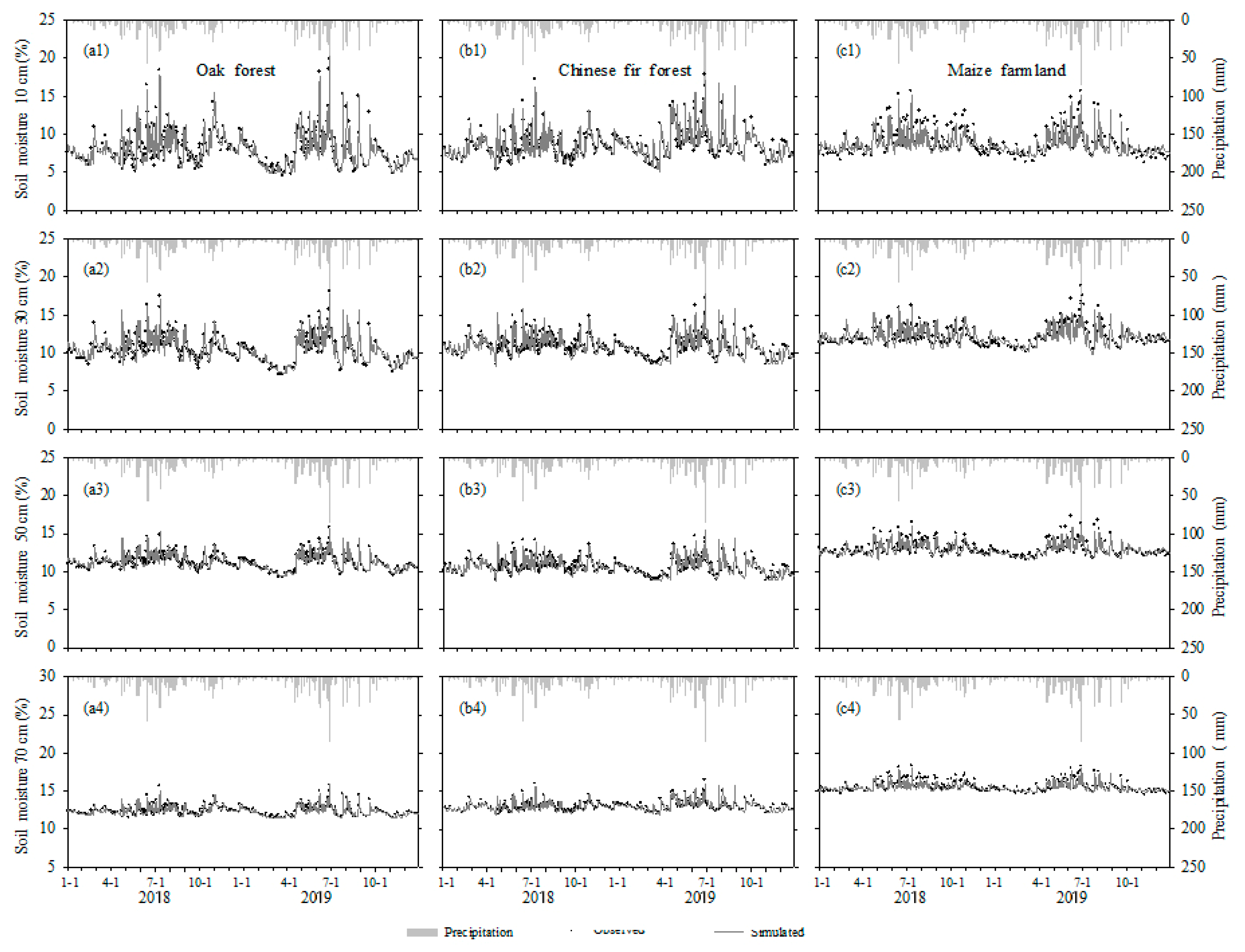
The time series of measured and simulated soil moisture at depths of 10, 30, 50, and 70 cm for the three plots are shown in Figure 2. The temporal variation of soil moisture is similar for the three stands, showing a distinct trend with the highest values during summer (especially from June to August). This trend is consistent with that of precipitation events, which slightly declines during September and reaches minimum values through winter and spring (November to February). Compared with the variability of soil moisture at the 70 cm layer, which at the depth of 10 cm is significant, with direct and rapid changes as reactions to rainfall. In the entire soil profile (0 cm to 80 cm), the average soil moisture ranged as follows: oak forest (10.55%) < Chinese fir forest (11.18%) < maize farmland (15.68%).

3.1.2. Validation of Modeled Results

Validation results showed the desired conformity between the simulated and measured data (Figure 2 and

Table 3. Statistical performance of CoupModel.

		Oak Forest					Chinese Fir Forest					Maize Farmland
Variable	Horizon/cm	R2	ME/%	RMSE/%	AverageObs. /%	n Obs.	R2	ME/%	RMSE/%	AverageObs. /%	n Obs.	R2	ME/%	RMSE/%	AverageObs. /%	n Obs.
Soil moisture	0–10	0.83	0.39	1.81	7.79	320	0.8	1.52	2.11	8.06	320	0.73	0.49	0.46	8.47	229
	10–20	0.88	0.3	2.19	13.71	320	0.86	0.86	1.89	16.21	320	0.74	0.52	3.84	20.07	229
	20–30	0.84	0.39	1.41	10.59	320	0.85	0.83	1.48	13.62	320	0.85	−0.83	1.41	15.98	229
	30–40	0.86	−0.16	1.4	9.25	320	0.81	−0.35	1.24	9.38	320	0.79	−0.20	0.68	15.50	229
	40–50	0.89	0.42	1.11	9.49	320	0.86	0.41	0.81	9.02	320	0.8	0.95	0.58	16.17	229
	50–60	0.91	−0.28	0.61	10.18	320	0.78	0.18	0.99	7.87	320	0.78	−0.13	1.33	18.22	229
	60–70	0.86	−0.02	1.38	10.86	320	0.83	0.26	1.22	12.26	320	0.87	−0.12	1.89	15.29	229
	70–80	0.91	−0.05	3.39	12.51	320	0.83	−0.1	2.28	13.03	320	0.86	−0.09	2.71	15.71	229
Throughfall	-	0.62	2.37 mm	4.51 mm	-	34	0.69	1.92 mm	4.2 mm	-	34	-	-	-	-	-

). The coefficient of determination for the linear regression (R²) between the observed and simulated soil moisture in the entire soil profile (0 cm to 80 cm) was 0.83–0.91 (p < 0.001) for oak forest but slightly lower for Chinese fir forest (0.78–0.86) and farmland (0.73–0.87). Generally, R² is useful for describing the difference between the simulated and observed dynamics of variables with cyclic fluctuations. In this study, R² is above 0.73 for all plots, indicating that CoupModel well simulates soil moisture. ME and RMSE reflect the deviation between the simulated values and measured values and, thus, facilitate the depiction of the irregular patterns of variables for soil moisture changes in response to infiltration events and drying processes. For the three plots, ME is −0.83 to 1.52%, with RMSE of 0.46–3.84%. We deduce that the deviation was small between the simulated and measure values, indicating that the model effectively captured the dynamic changes in soil moisture and that the simulation results were reliable.

Compared with soil moisture, simulated throughfall had disappointing measurements, with R² of only 0.62–0.69 possibly because of the small number of samples [29]. Wang [1313] suggested that such measurements can also be attributed to uncertainties in several parameters, such as Si max and LAI (Table 2).

3.1.3. Model Prediction

CoupModel successfully simulated soil moisture dynamics. However, several discrepancies were observed between the simulated and measured values. First, larger discrepancies were found between the simulated and measured soil moisture in the upper 10 cm of the soil than lower in the profile (Figure 2 and Table 3) because the upper layer was easily disturbed by environmental factors (e.g., microclimatology and animal or human activities). Except for the measurement error of FDR, it would be advisable to have an approach that directly considers the influence of the spatial variability of soil texture, land cover, slope, and meteorological conditions in estimation [23,26,27]. Second, uncertainty was higher during summer and autumn than during winter and spring in both the modeling and observation (Figure 2), not only because of the great variability of climate (such as that of rainfall, temperature, radiation, and even soil nutrient constraints), but also because of the rapid growth of plants and intense evapotranspiration, which intensify and accelerate soil water movement [27,28]. Third, the simulation results varied among different vegetation types. We used the same parameters to describe soil hydraulic properties for all plots but different parameters to describe the upper boundary conditions (soil surface and plant description, e.g., LAI, tree height, and root depth) for different plots. Fixed parameter values for each soil layer may not represent heterogeneous field conditions with highly variable water content within field replicates [23,26].

3.2. Simulated Water Balance Components

3.2.1. Precipitation

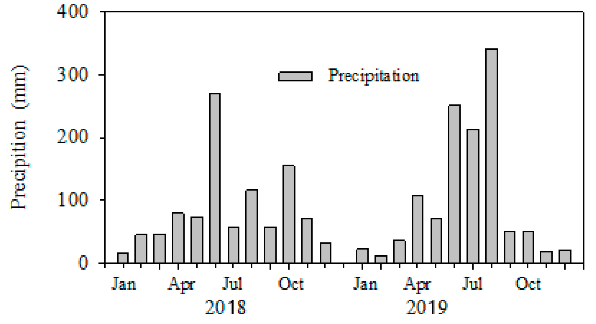
In Simian Mountain, the mean annual precipitation was 1096.7 mm (from 1951 to 2018). The precipitation data in Figure 3 indicated that rainfall was 1020 and 1194 mm in 2018 and 2019, respectively. Both years can be regarded as normal flow years. Torrential rain was mainly concentrated in June 2018, and large quantities of rain were also observed in July and August 2019, in which period most subsurface flow occurred, and groundwater recharge increased.

3.2.2. Canopy Interception

Figure 4 clearly shows a seasonal change in the distribution of interception (I). For the two forest stands, canopy interception generally increased in March and reached its maximum amount from June to August (35 mm to 63 mm), when rainfall was significant, and then gradually decreased in October (12 mm to 19 mm) and became very low from December to the following February. For the farmland plot, crop interception rose in May (about 20 mm), when maize seeds were sown, and fluctuated (23 mm to 36 mm) with the growth of crops. In China, researchers found that canopy interception was closely related to vegetation characteristics (e.g., forest structure, planting density, tree age, LAI, and coverage) and precipitation conditions (e.g., rainfall intensity and duration, and size and orientation of raindrops), generally ranging between 11.4% and 36.5% (between 134 and 626 mm) for forest ecosystems [38,39,40]. In our study, the average interception losses in the Chinese fir (24%) forestland was consistent with previous observations for the same species (fir, 23.6%) in similar climate in southern China by Sun [41] in 2018 and 2019. However, studies of the interception of oak have different findings. He [38] found that the average interception losses account for 16.5% of the total rainfall in oak forestland; Xue [39] reported a different value of 35.8%. The discrepancies between our results and those of other studies may be due to the different precipitations or experimental periods. In 2018 and 2019, the annual amount of simulated interception was 128 mm for the maize stand, 149 and 130 mm lower than those of the oak and Chinese fir forestlands (

Table 4. Simulated annual water balance (in mm) with CoupModel.

Year	Plot	Precipitation	Actual Evapotranspiration	Interception	Transpiration	Soil Evaporation	Deep Percolation	Change of Soil Water Storage
		(P) /mm	(ET) /mm (% P)	(I) /mm (% P)	(Et) /mm (% P)	(Es) /mm (% P)	(D) /mm (% P)	ΔS /mm (% P)
2018	Oak forest	1020	684 (67)	261 (26)	240 (24)	183 (18)	358 (35)	−22 (−2)
	Chinese fir forest	1020	670 (66)	243 (24)	219 (21)	208 (20)	368 (36)	−17 (−2)
	Farmland	1020	581 (57)	121 (12)	170 (17)	290 (28)	408 (40)	31 (3)
2019	Oak forest	1194	756 (63)	293 (25)	297 (25)	167 (14)	426 (36)	12 (1)
	Chinese fir forest	1194	731 (61)	274 (23)	269 (23)	189 (16)	441 (37)	22 (2)
	Farmland	1194	621 (52)	134 (11)	213 (18)	274 (23)	495 (41)	78 (7)
Average (2018–2019)	Oak forest	1107	720 (65)	277 (26)	268 (25)	175 (16)	392 (36)	−5 (−1)
	Chinese fir forest	1107	700 (63)	258 (24)	244 (22)	198 (18)	404 (37)	3 (0)
	Farmland	1107	601 (55)	128 (12)	192 (18)	282 (26)	451 (41)	55 (5)

). The possible reason was that the forests had two canopy layers and a long growing season and, thus, intercepted more rainfall than crops, which had only one layer with short plant height or growing season [12,13].

3.2.3. Plant Transpiration

Similar to interception (I), transpiration (E_t) also exhibits obvious seasonal pattern (Figure 4). Given that precipitation provides water for evapotranspiration whereas temperature determines intensity, they are the two main factors that affect transpiration. Forest plants regenerated new leaves in March, and the transpiration rate gradually grew to the peak in June and August (35 mm to 57 mm) with maximum rainfall and temperature. Afterward, the transpiration was then reduced by cold weather with low rainfall and temperature. However, from June to August, transpiration dramatically dropped in July (constantly at the 26 mm level), because little rainfall leaded to a rapid descent in soil moisture, which in turn restricted water supply for transpiration. During this period, evapotranspiration (ET) may generally be equal to or even greater than precipitation. During the experimental period, the simulated annual transpiration for the oak and Chinese fir forests was 268 and 244 mm, respectively, accounting for 25% and 22% of total precipitation (Table 4). These values are close to the previous estimations by Dai [40] and Liu [42] for broadleaved (18.8–26.0%) and coniferous (18.4–38.3%) forests in similar climate. For the farmland, the annual transpiration was only 192 mm (22% of total precipitation), indicating significantly less transpiration than that in the forest.

3.2.4. Soil Evaporation

The simulated monthly soil evaporation for each plot is presented in Figure 4. In contrast to the seasonal fluctuations of I and Et, soil evaporation (Es) remained relatively constant (9 mm to 22 mm every month) during growing season and modestly rose in winter and early spring. The simulated changes of I, Et, and Es showed that I and Et took large proportions of ET in growing season, whereas Es dominated ET before plants grew. Compared with the simulated annual evaporation in the farmland (282 mm, 26% of P), that in the forest stands was low, 175 mm for oak and 198 mm for Chinese fir (16% and 18% of P). These values significantly differed from the high I and Et in the forestlands. In our study, the simulated soil evaporation in the maize plot (47% of ET) was comparable with previous observations (37–45% of ET) by Zhao [22].

3.2.5. Deep Percolation

In contrast to evapotranspiration (ET), deep percolation (D) always abruptly changed (maximum of 200 mm) with rainstorm events (mainly in June 2018 and between June and August 2019). Water recharge is also intense in rainy season, but minimal in dry season (Figure 4). In 2018 and 2019, 408 and 495 mm deep percolation/drainage formed in the farmland, more than 40% of the gross precipitation. In contrast to the farmland, the oak (annual D = 392 mm) and Chinese fir (402 mm) forest plots presented similar distribution with lower deep percolation during the two-year period, accounting for only 36% and 37% of the total precipitation (Table 4). The deep percolation in the oak and Chinese fir forestlands was consistent with the modeled values (385.5 mm for broadleaved forest and 395.2 mm for coniferous forest) by Dai [40], but considerably higher than the observations (323.6 mm for wheat–maize farmland) by Zhu [43] in a region with similar climate. In this study, the lower boundary of soil was unsaturated, and the movement of water in the deep layer usually exhibited unsaturated flow based on unit gradient. Thus, the flow speed or unsaturated hydraulic conductivity was closely related to soil moisture. In the oak and Chinese fir forest plots, the soil moisture content was 12.51% and 13.03% at the 80 cm layer (Table 3), but it was 15.71% for the farmland; thus, unsaturated hydraulic conductivity was higher in the farmland and soil water flow moved faster and infiltrated deeper than in the forestlands.

3.2.6. Water Balance

The simulated monthly and annual sums of water balance components for the study plots are illustrated in Figure 4 and Table 4. Similar to the seasonal variation of precipitation, a clear tendency was observed in the monthly water balance components for the three plots. During the simulation period, actual evapotranspiration (ET), the sum of interception (I), transpiration (Et), and soil evaporation (Es) showed a distinct temporal variation with the highest values (110 mm to 128 mm) in June to August in growing season and the lowest values from December to the following February. For the farmland plot, the annual share of ET in relation to P was 55% (601 mm). In the oak and Chinese fir forest plots, however, ET annually contributed 65% and 63% of P (720 and 700 mm, respectively), 119 and 99 mm higher than that of the farmland (Table 4). The differences in the annual ET rates of vegetation types resulted in different transitions among the water balance components. In the experimental period, the results of a comparison of both forest sites were expected and generally agreed with the findings of Dai [40], who studied the effect of different forests on water budgets in similar climate conditions with the SWAT model. Dai [40] observed higher I and Et and lower Es and D for broadleaved forest than that for coniferous forest and the lowest ET and highest D for grassland. Liu [42] obtained similar results with TOPMODEL in the upstream of Yangtze River. Studies of water balance between farmland and forest sites in this region are scarce in terms of data covering the whole year, but similar studies in other areas are readily available. The results of long-term monitoring studies show that forests exhibit markedly higher canopy interception and transpiration than farmland; thus, I and Et are likely to be the dominating factors that affect water balance components [13,44].

3.3. Effect of Afforestation on Water Balance

3.3.1. Changes in Water Balance after Afforestation

This study indicated that a shift from cropland to forest would lead to an increase in canopy interception (I) and plant transpiration (Et) while a reduction in soil evaporation (Es) and/deep percolation (D)/groundwater recharge. First, annual interception increased (122 mm to 159 mm) after afforestation (Table 4). Compared with crops, trees had a large leaf area in our study sites, implying high canopy capacity for interception storage, and a low amount of precipitation directly reaching the ground, especially before crops were sown or the canopy closed [28]. Second, except for interception loss, annual transpiration from the forest stand was high, approximately 49 mm to 84 mm higher than that from the farmland (192 mm). The reason was that forests support great biomass with long growing periods, indicating that they may consume much water to supplement high transpiration. Moreover, forests can absorb water from great soil volume with a deep rooting system; thus, much water is available for transpiration [8,28]. Wang [13] and Zhang [44] propose that many factors that govern transpiration are favorable in forest sites. For example, trees in forest sites have large persistent leaf areas and high aerodynamic efficiency and thus facilitate plant transpiration. Third, although afforestation was modeled to increase vegetation transpiration and interception evaporation, it was also simulated to decrease soil evaporation compared with former arable land (Figure 3 and Table 4). For example, compared with the modeled soil evaporation from cropland in 2019, the soil evaporation decreased from about 85 mm to 104 mm, and the two stands only accounted for 61% and 69% of the farmland (274 mm), respectively. One possible reason is that forests have a canopy structure that substantially reduces wind speed and radiation and thereby limits soil evaporation [44]. Fourth, a 40 mm to 69 mm (10–14%) reduction in annual deep percolation was estimated after afforestation (Table 4). The probable reason was that most precipitation in forestlands was absorbed by the soil surface and rapidly diffused by evaporation or transpiration after afforestation, thereby decreasing infiltration depth and soil water content below the infiltration depth [27,28]. Therefore, on sites with low plant available soil water capacity and with roots that have no access to the water table, a change in land use from cropland to forest may negatively affect groundwater recharge.

3.3.2. Effect of Tree Species

Water balance is strongly influenced by climate, soil properties, and the tree species selected for afforestation [11]. In this study, the two forest stands are located on the same soil type and share climate and pre-afforestation history. Thus, tree species is a significant factor in the hydrological fluxes. The highest interception and transpiration occurred in the oak stand, with the annual values 19 and 24 mm higher than those for Chinese fir of the same age (128 and 192 mm). Leaf area is an important factor that determines interception and transpiration by vegetation [7,13]. Similar to Chinese fir, oak is an evergreen species, but it had a larger leaf area (Table 2) with higher interception storage capacity and a larger evaporation area, which enhanced the interception loss. Transpiration at the oak stand was high probably because the biomass was increased by naturally regenerated seedlings and saplings in addition to the sub-canopy layer formed in the stand [7]. In addition, our model calculations indicated that the decline in water recharge was greater at the oak forest stand (22 mm) than in the Chinese fir forest (17 mm) in 2018 mainly because of the higher water consumption of oak. From the perspective of water conservation, the oak forest at its current density failed to store much soil water and generated no more recharge of groundwater because of its minimal deep percolation. In turn, the lack of soil water adversely affected the growth of trees and the land productivity. Thus, when drinking water is derived from groundwater reservoirs in such areas in large afforestation projects, tree species should be considered, particularly when such projects aim to improve the quantity of water that infiltrates the groundwater. Furthermore, soil and water conservation measures must be applied scientifically when farmland is converted to forest in TGRA in China, especially in oak forests with high density.

4. Conclusions

Based on field measurements in 2018 and 2019, a physical process-based model (CoupModel) was applied to simulate water balance in three vegetation types, namely, oak (Lithocarpus glaber) forest, Chinese fir (Cunninghamia. lanceolata) forest, and maize farmland (Zea mays), in Simian Mountain in the terminal section of TGRA. The simulated values of soil moisture were fairly consistent with the measured ones, with a determination coefficient (R²) of 0.73–0.91. This result indicates that CoupModel can successfully demonstrate the complex interactions between hydrological processes in the SVAT system. Evapotranspiration was the main output of water balance, with a percentage of up to 61%, and was ranked as follows: oak forest (720 mm/y) > Chinese fir forest (700 mm/y) > maize farmland (600 mm/y). However, the annual simulated deep percolation decreased by 60 and 47 mm for oak and Chinese fir forest compared with that for farmland (452 mm/y) mainly because of increased interception (122–159 mm/y) and transpiration (49–84 mm/y) after afforestation. The simulations indicated that vegetation type significantly influenced the magnitude of water balance components, calling for further attention to the selection of regrown tree species in the planning for afforestation projects, particularly for those who aim to improve the quantity of water infiltrating groundwater. Furthermore, soil and water conservation measures should be applied scientifically when converting farmland to forest in this area, especially in oak forests with high density.

References

- Wu, J.G.; Huang, J.H.; Han, X.G.; Gao, X.M.; He, F.L.; Jiang, M.X.; Jiang, Z.G.; Primack, R.B.; Shen, Z.H. The Three Gorges Dam: An ecological perspective. Front. Ecol. Environ. 2004, 2, 241–248. [Google Scholar] [CrossRef]
- Zhang, Q.F.; Lou, Z.P. The environmental changes and mitigation actions in the Three Gorges Reservoir region, China. Environ. Sci. Policy 2011, 14, 1132–1138. [Google Scholar] [CrossRef]
- Xiao, W.F.; Lei, P.J. Spatial distribution, disturbance and restoration of forests in the Three Gorges Reservoir region. Resour. Environ. Yangtze Basin 2004, 13, 138–144. [Google Scholar]
- Cheng, J.H.; Zhang, H.J.; Wang, W.; Zhang, Y.Y.; Chen, Y.Z. Changes in Preferential Flow Path Distribution and Its Affecting Factors in Southwest China. Soil Sci. 2011, 176, 652–660. [Google Scholar] [CrossRef]
- Lu, W.X.; Zhang, H.J.; Cheng, J.H.; Wang, H.Y.; Li, J.Q.; Wang, W. Effect of a hedgerow agroforestry system on soil proper-ties of sloping cultivated lands in the Three-Gorges area in China. J. Food Agric. Environ. 2012, 10, 1368–1375. [Google Scholar]
- Eckhardt, K.; Breuer, L.; Frede, H.-G. Parameter uncertainty and the significance of simulated land use change effects. J. Hydrol. 2003, 273, 164–176. [Google Scholar] [CrossRef]
- Granier, A.; Biron, P.; Lemoine, D. Water balance, transpiration and canopy conductance in two beech stands. Agric. For. Meteorol. 2000, 100, 291–308. [Google Scholar] [CrossRef]
- Chen, H.S.; Shao, M.A.; Li, Y.Y. The characteristics of soil water cycle and water balance on steep grassland under natural and simulated rainfall conditions in the Loess Plateau of China. J. Hydrol. 2008, 360, 242–251. [Google Scholar] [CrossRef]
- Leauthaud, C.; Kergoat, L.; Hiernaux, P.; Grippa, M.; Musila, W.; Duvail, S.; Albergel, J. Modelling the growth of floodplain grasslands to explore the impact of changing hydrological conditions on vegetation productivity. Ecol. Model. 2018, 387, 220–237. [Google Scholar] [CrossRef]
- Rosenqvis, L.; Hansen, K.; Vesterdal, L.; van der Salm, C. Water balance in afforestation chronosequences of common oak and Norway spruce on former arable land in Denmark and southern Sweden. Agric. For. Meteorol. 2010, 150, 196–207. [Google Scholar] [CrossRef]
- Pathak, D.; Whitehead, P.G.; Futter, M.N.; Sinha, R. Water quality assessment and catchment-scale nutrient flux modeling in the Ramganga River Basin in north India: An application of INCA model. Sci. Total. Environ. 2018, 631, 201–215. [Google Scholar] [CrossRef] [PubMed]
- Wang, L.; Wei, S.P.; Horton, R.; Shao, M.A. Effects of vegetation and slope aspect on water budget in the hill and gully region of the Loess Plateau of China. Catena 2011, 87, 90–100. [Google Scholar] [CrossRef]
- Wang, L.; Wang, S.P.; Shao, H.B.; Wu, Y.J.; Wang, Q.J. Simulated water balance of forest and farmland in the hill and gully region of the Loess Plateau in China. Plant Biosyst. 2012, 146, 226–243. [Google Scholar] [CrossRef]
- Doerr, S.H.; Ritsema, C.J.; Dekker, L.W.; Scott, D.F.; Carter, D. Water repellence of soils: New insights and emerging research needs. Hydrol. Process. 2007, 21, 2223–2228. [Google Scholar] [CrossRef]
- Farley, K.A.; Jobbágy, E.G.; Jackson, R.B. Effects of afforestation on water yield: A global synthesis with implications for poli-cy. Glob. Chang. Biol. 2005, 11, 1565–1576. [Google Scholar] [CrossRef]
- Sun, G.; Zhou, G.Y.; Zhang, Z.Q.; Wei, X.H.; McNulty, S.G.; Vose, J.M. Potential water yield reduction due to forestation across China. J. Hydrol. 2006, 328, 548–558. [Google Scholar] [CrossRef]
- Bosch, J.M.; Hewlett, J.D. A review of catchment experiments to determine the effect of vegetation changes on water yield and evapotranspiration. J. Hydrol. 1982, 55, 3–23. [Google Scholar] [CrossRef]
- Hatten, J.A.; Segura, C.; Bladon, K.D.; Hale, V.C.; Ice, G.G.; Stednick, J.D. Effects of contemporary forest harvesting on sus-pended sediment in the Oregon Coast Range: Alsea Watershed Study Revisited. For. Ecol. Manag. 2018, 408, 238–248. [Google Scholar] [CrossRef]
- Van der Salm, C.; Denier van der Gon, H.; Wieggers, R.; Bleeker, A.; Van den Toorm, A. The effect of afforestation on water recharge and nitrogen leaching in the Netherlands. For. Ecol. Manag. 2006, 221, 170–182. [Google Scholar] [CrossRef]
- Hansen, K.; Rosenqvist, L.; Vesterdal, L.; Gundersen, P. Nitrate leaching from three afforestation chronosequences on former arable land in Denmark. Glob. Chang. Biol. 2007, 13, 1250–1264. [Google Scholar] [CrossRef]
- Zhou, G.Y.; Morris, J.D.; Yan, J.H.; Yu, Z.Y.; Peng, S.L. Hydrological impacts of reaforestation with eucalyptus and indige-nous species: A case study in southern China. For. Ecol. Manag. 2002, 167, 209–222. [Google Scholar] [CrossRef]
- Zhao, N.N.; Liu, Y.; Cai, J.B.; Yu, F.L.; Li, C.Z. Research on soil evaporation of summer maize by field measurement and model simulation. Trans. Chin. Soc. Agric. Eng. 2012, 28, 66–73. [Google Scholar]
- Zhang, S.; Lövdahl, L.; Grip, H.; Jansson, P.-E.; Tong, Y. Modelling the effects of mulching and fallow cropping on water balance in the Chinese Loess Plateau. Soil Tillage Res. 2007, 93, 283–298. [Google Scholar] [CrossRef]
- Jansson, P.E.; Karlberg, L. Coupled Heat and Mass Transfer Model for Soil-Plant-Atmosphere Systems; Royal Institute of Technology, Dept. of Civil and Enviromental Engineering: Stockholm, Sweden, 2004; Volume 251, pp. 211–218. [Google Scholar]
- Jansson, P.-E. CoupModel: Model Use, Calibration, and Validation. Trans. ASABE 2012, 55, 1337–1346. [Google Scholar] [CrossRef]
- Ladekarl, U.L.; Rasmussen, K.R.; Christensen, S.; Jensen, K.H.; Hansen, B. Groundwater recharge and evapotranspiration for two natural ecosystems covered with oak and heather. J. Hydrol. 2005, 300, 76–99. [Google Scholar] [CrossRef]
- Christiansen, J.R.; Elberling, B.; Jansson, P.E. Modelling water balance and nitrate leaching in temperate Norway spruce and beech forests located on the same soil type with the CoupModel. For. Ecol. Manag. 2006, 237, 545–556. [Google Scholar] [CrossRef] [Green Version]
- Schmidt-Walter, P.; Lamersdorf, N.P. Biomass Production with Willow and Poplar Short Rotation Coppices on Sensitive Areas—the Impact on Nitrate Leaching and Groundwater Recharge in a Drinking Water Catchment near Hanover, Germany. BioEnergy Res. 2012, 5, 546–562. [Google Scholar] [CrossRef] [Green Version]
- Wu, S.H.; Jansson, P.-E.; Zhang, X.Y. Modelling temperature, moisture and surface heat balance in bare soil under seasonal frost conditions in China. Eur. J. Soil Sci. 2011, 62, 780–796. [Google Scholar] [CrossRef]
- Zhou, J.; Kinzelbach, W.; Cheng, G.D.; Zhang, W.; He, X.B.; Ye, B.S. Monitoring and modeling the influence of snow pack and organic soil on a permafrost active layer, Qinghai–Tibetan Plateau of China. Cold Reg. Sci. Technol. 2013, 90, 38–52. [Google Scholar] [CrossRef]
- Brooks, R.H.; Corey, A.T. Hydraulic Properties of the Porous Media. Hydrology Paper No.3. Ph.D. Thesis, Colorado State University, Fort Collins, CO, USA, 1964. [Google Scholar]
- Richards, L.A. Capillary conduction of liquids through porous mediums. Physics 1931, 1, 318–333. [Google Scholar] [CrossRef]
- Mualem, Y. A new model for predicting the hydraulic conductivity of unsaturated porous media. Water Resour. Res. 1976, 12, 513–522. [Google Scholar] [CrossRef] [Green Version]
- Monteith, J.L.; Kavanau, R.B.J.L. The State and Movement of Water in Living Organisms. Symposium of the Society for Ex-perimental Biology. by G. E. Fogg. Q. Rev. Biol. 1967, 42, 87–88. [Google Scholar]
- Manzi, A.O.; Planto, S. Implentation of the ISBA parametrization scheme for land surface processes in a GCM-an annual cycle experiment. J. Hydrol. 1994, 155, 37–46. [Google Scholar] [CrossRef]
- Gustafsson, D.; Lewan, E.; Jansson, P.-E. Modeling Water and Heat Balance of the Boreal Landscape—Comparison of Forest and Arable Land in Scandinavia. J. Appl. Meteorol. 2004, 43, 1750–1767. [Google Scholar] [CrossRef]
- Verstraeten, W.W.; Veroustraete, F.; Feyen, J. Assessment of Evapotranspiration and Soil Moisture Content Across Different Scales of Observation. Sensors 2008, 8, 70–117. [Google Scholar] [CrossRef] [Green Version]
- He, C.Q.; Xue, J.H.; Wu, Y.B.; Zhang, L.Y. Application of a revised Gash analytical model to simulate subalpine Quercus aq-uifolioides forest canopy interception in the upper reaches of Minjiang River. Acta Ecol. Sin. 2010, 30, 1125–1132. [Google Scholar]
- Xue, J.H.; Hao, Q.L.; Wu, Y.B.; Liu, X.L. Relationship among canopy interception, throughfall and precipitation in three types of subalpine forest communities. J. Nanjing For. Univ. (Nat. Sci. Ed.) 2008, 32, 9–13. [Google Scholar]
- Dai, J.F.; Chen, J.Z.; Cui, Y.L.; He, Y.Q.; Ma, J.G. Impact of forest and grass ecosystems on the water budget of the catchments. Adv. Water Sci. 2006, 17, 435–443. [Google Scholar]
- Sun, X.Y.; Wang, G.X.; Li, W.; Liu, G.S.; Lin, Y. Measurements and modelling of canopy interception in the Gongga Mountain subalpine succession forest. Adv. Water Sci. 2011, 22, 23–29. [Google Scholar]
- Liu, H.M.; Tao, S.H.; Chen, Y.Q.; Zhou, H.B.; Wang, J.G. Simulation study on the effects of vegetation on basin water balance. Meteorol. Environ. Res. 2010, 1, 62–68. [Google Scholar]
- Zhu, B.; Zhou, M.H.; Kuang, F.H.; Wang, T. Measurement and simulation of nitrogen leaching loss in hillslope cropland of purple soil. Chin. J. Eco-Agric. 2013, 21, 102–109. [Google Scholar]
- Zhang, L.; Dawes, W.R.; Walker, G.R. Response of mean annual evapotranspiration to vegetation changes at catchment scale. Water Resour. Res. 2001, 37, 701–708. [Google Scholar] [CrossRef]
Figure 1.
Field Site (there are two plots: oak site and Chinese fir site, respectively, and one maize site).
Figure 2.
Daily soil moisture: frequency domain reflectometry (FDR) measurements (black circles) and simulated values (gray solid line). Each column from left to right represents oak forest, Chinese fir forest, and maize farmland, respectively. Horizontal (a1–c1,a2–c2,a3–c3,a4–c4) represents soil moisture in 10 cm, 30 cm, 50 cm, and 70 cm soil depth, respectively.
Figure 3.
Monthly precipitation in experimental plots.
Figure 4.
Simulated monthly water fluxes for three plots (drainage and groundwater recharge (deep percolation) are represented by negative values.)