
A Comprehensive Case Study of Data-Driven Methods for Robust Aircraft Sensor Fault Isolation


1
Department of Engineering, University of Perugia, Via G. Duranti, 67, 06125 Perugia, Italy
2
Department of Mechanical and Aerospace Engineering, West Virginia University, Morgantown, WV 26506-6106, USA
*
Author to whom correspondence should be addressed.
Sensors 2021, 21(5), 1645; https://doi.org/10.3390/s21051645
Submission received: 23 December 2020
/
Revised: 16 February 2021
/
Accepted: 22 February 2021
/
Published: 26 February 2021
(This article belongs to the Section Fault Diagnosis & Sensors)
Abstract
:Recent catastrophic events in aviation have shown that current fault diagnosis schemes may not be enough to ensure a reliable and prompt sensor fault diagnosis. This paper describes a comparative analysis of consolidated data-driven sensor Fault Isolation (FI) and Fault Estimation (FE) techniques using flight data. Linear regression models, identified from data, are derived to build primary and transformed residuals. These residuals are then implemented to develop fault isolation schemes for 14 sensors of a semi-autonomous aircraft. Specifically, directional Mahalanobis distance-based and fault reconstruction-based techniques are compared in terms of their FI and FE performance. Then, a bank of Bayesian filters is proposed to compute, in flight, the fault belief for each sensor. Both the training and the validation of the schemes are performed using data from multiple flights. Artificial faults are injected into the fault-free sensor measurements to reproduce the occurrence of failures. A detailed evaluation of the techniques in terms of FI and FE performance is presented for failures on the air-data sensors, with special emphasis on the True Air Speed (TAS), Angle of Attack (AoA), and Angle of Sideslip (AoS) sensors.
1. Introduction
Fault Diagnosis (FD) is a term that describes the general problem of detecting and isolating faults in physical components or in the instrumentation of a system [1]. A broad class of FD methods is based on the concept of Analytical Redundancy (AR) [2]. The essence of AR methods lies in the comparison of the behavior of the system with the response of a mathematical model. Inconsistency between the actual and model response is considered a symptom of a possible failure. An FD scheme elaborates this information in real time to detect and isolate faults.
Mathematical models play a central role in AR-based FD; these are derived from either physical laws governing the dynamics of the system or are inferred directly from experimental data exploiting system identification techniques [3].
In the last 30 years, FD has been widely investigated, and many techniques have been proposed. Considering model-based approaches, the main research directions can be coarsely categorized as fault detection filters, parity-space schemes, diagnostic observers, and parameter estimation [1]. Classic methods dealing with model-based approaches can be found in [4,5,6,7,8,9]. More recently, approaches based on optimal criteria [10,11] and extensions to nonlinear [12], hybrid [13], and distributed systems [14] have been proposed. A collection of successful applications of model-based FD was presented in [15].
Data-based approaches are preferable instead in case the system dynamics is not precisely known and/or when the system input-output physical relations are too complex [16]. Currently, thanks to the advances in ICT technologies in both hardware and software, substantial amounts of data are available for continuous monitoring and FD of engineering systems. This generated a great interest in FD techniques capable of handling large amounts of data. In this context, the most established and widespread techniques are Principal Component Analysis (PCA), Independent Component Analysis (ICA), Partial Least Squares (PLS), Fisher Discriminant Analysis (FDA), the Subspace-Aided approach (SAP), as well as their recent advancements [17]. Remaining in the data-based domain, FD diagnostic systems based on neural networks [18], computational intelligence [19], and machine learning [20,21] have attracted substantial interest in very recent years. Specifically, in the aviation and flight control systems community, there is abundant technical literature that clearly shows that the main reason for catastrophic accidents can be attributed, ultimately, to failures and/or malfunction of sensors, control surfaces, or components of the propulsion system, as reported in [22,23]. This explains the critical need for on-board FD systems able to promptly detect and identify the faulty components and, next, to enable a predetermined online failure recovery strategy [24]. Typically, hardware redundancy (featuring multiple sensors or actuators with the same function) and simple majority voting schemes are used to cope with FD. Although these methods are widespread, there is an increasing number of applications where the additional cost, weight, and size of the components are major constraints, such as small and autonomous flying vehicles. For these applications, AR-based FD methods are appealing approaches to increase flight safety. An excellent review on the state-of-the-art of AR-based FD methods in aerospace systems can be found in [25].
Regardless of the approach, the performance of an FD system is strictly related to the level of modeling uncertainty and measurement noise, whose presence implies that in fault-free conditions, the residual signals might significantly deviate statistically from zero. This entails that residuals must be robust with respect to uncertainties where the robustness of a residual is defined as the degree of sensitivity to faults compared to the sensitivity to uncertainty and noise [26]. Robustness issues become evident when dealing with experimental flight data [27,28,29,30,31]. Indeed, experimental data are affected by several additional sources of uncertainty such as, but not limited to, signal synchronization and quantization errors and imperfect positioning and calibration of the sensors [32,33]. Therefore, a fundamental step before the deployment of an FD scheme is its validation with actual flight data. Despite the relevance of these aspects in the mentioned studies, the problem of a detailed performance evaluation and comparison of Fault Isolation (FI) and Fault Estimation (FE) schemes using multi-flight data has been rarely fully addressed.
Building on the last considerations, the present study is entirely devoted to the setup and the quantitative comparison of well-known FI and FE methods using experimental sensor flight data. Specifically, different consolidated data-driven FI and FE schemes are applied to evaluate their performance on a set of 14 primary sensors of a semi-autonomous Tecnam P92 aircraft [34].
In the effort, experimental linear regression models of the sensors’ response are identified from correlated measurements using multivariate linear regression techniques [3]. The identified models provide a natural set of primary residuals; however, the faults’ directional properties are often not optimized to be used for sensor FI [35,36]. For this reason, enhanced residuals are derived by applying a linear transformation that allows better separation between the fault directions. The approach proposed in [37] that optimizes fault directions separation taking also into account experimental modeling errors is herein implemented.
Sensor FI is then performed using two different approaches. The first approach associates the fault with the sensor providing the smaller directional distance compared to the sensor fault directions [35]; the second approach, instead, is based on the reconstruction-based method proposed in [38].
A comprehensive (offline) analysis based on multi-flight data is performed to derive quantitative Fault Isolation (FI) and Fault Estimation (FE) performance as a function of the fault amplitudes.
Next, another study is performed to assess online sensor FI performance by monitoring the temporal history of the residuals and, using this information, to increase or decrease the belief in a fault hypothesis over time. For this purpose, a bank of recursive Bayesian filters is designed to infer in-flight sensors’ fault probabilities. During online operation, a fault is declared when a fault probability reaches a defined threshold. This allows the computation of FI delays. The accumulated evidence in the probabilistic filters allows more reliable fault isolation, decreasing the false alarm rate at the expense of a small and acceptable delay in the diagnosis.
A detailed evaluation of offline and online FD performance is presented for failures on the air data sensors, including the True Air Speed (TAS, ), the Angle of Attack (AoA, ), and the Angle of Sideslip (AoS, ).
The present study is application oriented; therefore, the main contribution is not the development of a novel FD technique, but, rather, the design of consolidated data-driven sensor FD schemes and the quantitative evolution of fundamental quantities such as the fault isolation percentage, fault reconstruction accuracy, and in-flight fault isolation delays using multi-flight validation data. Therefore, the study provides a clear picture of the required design effort along with the achievable performance using consolidated FD schemes.
The paper is organized as follows. Section 2 introduces linear regression models for sensors’ fault diagnosis; Section 3 introduces the FI and FE methods based on primary residuals, while Section 4 introduces the FI and FE methods based on transformed residuals. Section 5 introduces the Bayesian filters for online FI. Section 6 describes the multi-flight data, while Section 7 deals with the identification of experimental models. FI and FE results on validation data are discussed in Section 8 and Section 9. Concluding and summary remarks are provided in Section 10.
2. Models for Sensor Fault Diagnosis
In this study, a set of potentially faulty sensors is considered. The corresponding signals are concatenated in a vector ; is another vector of signals functionally correlated with such as control inputs, set-points, and other sensor measurements (assumed not to be faulty). It is assumed that in fault-free conditions, the sensor measurements can be expressed in linear regression form as a function of and , that is:
where and are the coefficients of the linear combination and characterizes modeling nonlinearity, uncertainty, and measurement noise concerning the i-th sensor. For simplicity, the linear models in (1) are rearranged as:
where and . Putting the above equations together, we get the following vector expression:
where and are constant matrices to be estimated from data (as discussed in Section 7). Model (3) has been widely used in the literature for estimating a sensor signal as a function of other correlated measurements, as shown, for instance, in [35,39,40,41,42]. The linear terms in (3) provide a linear estimation of the signals that are defined as:
The consistency of the measurements are monitored through the vector of the primary residuals that is defined as follows:
Substituting (4) into (5) leads to:
where is the identity matrix and . Using again (3) and (4) in (5), it is immediate to verify that:
In other words, in fault-free conditions, the vector of the primary residuals is equal to the modeling error.
Sensor Fault Modeling
In this study, an additive (single) failure on a generic (i-th) sensor of is considered. Without any loss of generality, the failure can affect every single sensor. In the presence of a sensor failure, the vector is replaced by its “faulty version”, that is:
where is the i-th column of the identity matrix . is an arbitrary scalar, a function of time, modeling the fault shape; thus, is zero before the fault occurrence and different from zero, starting from the “fault time instant” . In this study, we consider a step fault:
where is the fault amplitude associated with the i-th sensor.
3. Sensor FI and FE Based on Primary Residuals
The first FI scheme is derived directly from the analysis of the primary residual vector in (6) in the presence of a sensor fault. Substituting the faulty vector (8) in (6) leads to the faulty residual:
Next, substituting in (10) the conditions (7) results in:
where the vector is the i-th column of the matrix . Vector is known as the “fault signature” or the “fault direction” associated with the sensor fault . In the theoretical case of zero modeling error in (11), this results in:
In other words, the vector is exactly parallel to vector . This directional information can be used for sensor fault isolation purposes.
3.1. Mahalanobis Distance-Based FI and FE
This technique exploits the directional property of the primary residuals in (12) to formulate a sensor FI hypothesis [43]. Specifically, in the presence of a fault , Equation (12) implies that the residual vector assumes a specific known direction in the residual space given by the i-th column vector of matrix . By taking advantage of this fault directional property, it is possible to identify the faulty sensor by comparing the direction of the current residual vector with the known directions and assigning the fault to the sensor whose direction is the closest to the direction. In practice, this FI logic is implemented as follows. As the first step, in order to be independent of the fault amplitude, both the residual and the sensor fault directions are normalized to a unity norm. Specifically, at each instant k, the normalized residual () is computed as , while the normalized fault directions () are defined as . Next, since the faults can have either a positive or a negative amplitude, it was deemed necessary to introduce negative normalized fault directions (), implying that the overall number of fault directions is . The distance between the normalized residual and the normalized fault directions can be measured using different norms such as the Euclidean distance, the angular distance, or the Mahalanobis distance [44,45]. In this study, we selected the Mahalanobis distance since this approach allows accounting for modeling error information derived from experimental data. The error matrix of the differences between the normalized residual and the normalized fault directions is defined as:
where the first columns are associated with positive faults and the last with negative faults. Next, the Mahalanobis distance associated with the columns of is defined as:
where is the covariance matrix of the residuals (for its computation, see Note 1). At each sample time instant k (following a fault detection), the FI is performed associating the fault with the sensor leading to the minimum value of the distances in (14). That is, defining as:
then the faulty sensor index is identified as follows:
The amplitude of the fault is positive for , and it is negative for . Once a fault has been associated with the sensor , its amplitude can be directly estimated considering the -th component of the primary residual vector . In fact, from (11), this results in:
Next, since by construction, , this results in:
In other words, provides a direct (noisy) estimation of the fault amplitude defined in (9), that is:
3.2. Reconstruction-Based FI and FE
Another approach for FI and FE is the well-known reconstruction-based method [38,46,47]. In this approach, for each fault direction , the fault amplitude, at time instant k, is estimated by computing the fault amplitude that minimizes the norm-two of the reconstruction errors defined as:
The optimal values for are derived by computing the minimum of the quadratic form (20) with respect to the scalar . This leads to the closed-form solution:
It is observed that the fault amplitude estimation provided by (21) can be either positive or negative, implying that the reconstruction-based approach handles both positive and negative faults. The faulty sensor is then isolated associating the fault with the sensor leading to the minimum of the “reconstructed” errors achieved substituting the fault estimates (21) in (20). Therefore, the sensor fault index is:
Similar to (19), the estimated fault amplitude is:
Note 1: The residual noise covariance matrix in (14) depends on the modeling uncertainty in (7), which is very difficult to characterize “a priori”. For this reason, was estimated from the experimental data. From (7), it is inferred that in fault-free conditions, the relationship holds. This allows estimating as the sample covariance matrix of the residual vector inferred from experimental flight data in fault-free conditions. The experimental matrix is therefore:
Note 2: In this effort, we assumed that faults originate from sensors in an additive fashion. Under this hypothesis, it is possible to isolate the faulty sensor by analyzing the fault direction of the residual signals as shown in Equation (9). It is worth emphasizing that primary residuals can also be affected by the occurrence of generic internal system faults that in turn produce a specific fault signature on the residuals. In the case of internal faults, it is necessary to reconstruct the roots of the fault symptoms in the subsystems that constitute a complex system in order to be able to isolate the faulty component. In the event an internal fault produces a signature identical to those of a sensor fault, they would not be distinguishable by our scheme. The isolation of internal faults requires the knowledge of the internal dynamics of the subsystems and its cause-effect relationships. This problem, although interesting, is beyond the scope of this study, which is limited to addressing the sensor fault isolation problem. An interesting review on the cause and fault propagation can be found in [48].
4. Sensor FI and FE Based on Transformed Residuals
Primary residuals are not optimized from an FI point of view. For this reason, they are usually processed by applying transformations to achieve suitable new fault directions that facilitate the FI. An extensive literature on transformed directional residuals techniques is available. One of the first applications is the the Beard–Jones filter [13], essentially a Luenberger observer whose gains are selected so that the directions of the residuals can be advantageously used to identify faulty sensors. In [49], taking advantage of the properties of un-observability subspaces, a set of residual transformations that are unaffected by all faults except one was proposed. In this context, the methodology outlined in [36] is also relevant, where the interaction between directional residuals and fault isolation properties was analyzed.
The FI methodology proposed in [37] was considered in this effort because it provides optimized robust performance considering the directional properties of the residual noise covariance matrix . This feature is particularly important when dealing with experimental noisy data. In the approach in [37], a linear transformation of the primary residual vector is introduced to provide optimized performance with respect to noise immunity. A transformed residual with the same number of elements of is defined as:
where is the transformation matrix to be computed. Considering (25), the new fault directions associated with are the columns of the matrix:
The covariance of is by definition:
where the matrix is computed applying the method proposed in [37]. Considering this approach, let and be two symmetric matrices. Assuming positive definite, it can be shown that there exists a matrix such that:
where and are the solutions of the generalized eigenvalue problem. Specifically, the columns of are the eigenvectors of the matrix , while the columns of are the corresponding eigenvalues. In the present study, setting , , and , Equations (28) and (29) become, respectively:
Relationship (30) implies that the noise covariance matrix of the transformed residuals in (27) is spherical, that is . This property is critical since in the presence of a spherical symmetry noise, the optimal decision line between two fault directions is simply the bisector [50]. Thus, this property will be exploited for the design of the FI algorithm in Section 4.1.
As explained in Note 1, the matrix is estimated using the experimental in (24), and the generalized eigenvalues are derived using commercially available scientific software.
4.1. Transformed Residuals Based on FI and FE
Fault isolation based on the transformed residual is performed using the same approaches used for the primary residuals in Section 3.1 and Section 3.2. Specifically, defining the new transformed residual directions as the columns of the matrix , the transformed error matrix is defined as:
where is the normalized transformed residual derived from and are the new normalized transformed fault directions derived from . The distance errors associated with the columns of the matrix are defined as:
The fault isolation index is determined by applying the same technique introduced in Section 3.1, that is:
It is observed that the decision method (34) based on the Euclidean distances (33) is equivalent to treating as the decision line the bisectors between the directions in (32), which, in the case of spherical noise (), are also optimal for testing fault isolation [50].
The faulty sensor is isolated applying (16) to derived from (34). Finally, the fault amplitude is estimated using again (19), that is:
Note 3: In [37], it was shown that the best performances are achieved in the case that the transformation matrix leads to the diagonalization, not only of the noise covariance matrix , but also of the transformed fault direction matrix . This may be possible only if the number of residuals is larger than the number of sensors. Alternatively, approximated robust FI methods based on optimality concepts as those in [35,51] can be applied.
4.2. Transformed Residuals with Reconstruction-Based FI and FE
Consistent with the approach of Section 3.2, the reconstruction error for transformed residuals is defined as:
while the reconstructed fault amplitude is:
Fault isolation is again performed by computing the minimum of the errors in (36); in other words, the fault isolation index is:
Finally, similar to (23), the estimated fault is:
5. Bayesian Filtering for Online Fault Isolation
The FI approaches described in Section 3 and Section 4 are based on a decision method that isolates the faulty sensor as the one providing the minimum of a specific error measure inferred from the residual. This FI logic is based only on information at the current sample time k and does not take into account the history of the residuals in the previous instants. On the other side, this information is useful for increasing or decreasing the belief of the FI decision over time.
In this paper, we propose a Bayesian Filter (BF) approach for managing the stream of information coming from sensors’ measurements. Specifically, we implemented the so-called “discrete Bayes filter” proposed in [52]. This filter is essentially a recursive algorithm used to estimate the distribution of a discrete probability function. This type of filter was selected because it builds on a very solid and comprehensible theoretical background; an introduction to the Bayesian decision theory can be found in [53]. In the present study, the estimated distribution models the probability (belief) that a generic sensor is faulty. The BF infers sensor fault probabilities by processing recursively the error information defined in (14), (20), (33) and (36) for the different methods.
Two possible operational statuses are assumed for the sensors. State indicates the events for which the i-th sensor is faulty, while state the event for which it is not faulty. Let be the likelihood function representing the probability of observing an error given that the i-th sensor is faulty; a similar definition holds for . According to Bayes’ theorem, the posterior fault probabilities are given by:
where and are the a priori fault and non-fault probabilities, respectively, for sensor i. A key step in the above inference mechanism is the definition of the likelihood functions . These have to be designed to model the probability of experiencing a distance error given that the i-th sensor is faulty; therefore, their distribution needs to be maximum for and should decrease as increases. Similar reasoning applies to . This behavior is captured by the following likelihood functions [54,55,56,57]:
where the parameters are used to regulate the shape of the probability functions. At each time step, following the computation of the posterior probabilities (40), the a priori probabilities are updated recursively using:
to propagate the current probability information to the next time step. In this study, the probabilistic filters are activated immediately after a fault is detected at . At instant , it is assumed that all the sensors have the identical probability to be faulty; in other words, the filters are initialized with:
5.1. Probabilistic (Online) Fault Isolation Method
The recursive BF probabilities are employed for online FI, which is associated with in-flight conditions. Following a fault detection at , the fault is assigned to the sensor whose fault probability first reaches a defined threshold. If exceeds the threshold, the FI scheme has “good confidence” that a fault has occurred on the i-th sensor. Therefore, a failure on that sensor is declared. In this study, the threshold was empirically set at 0.7 (70%); see Note 4.
5.2. Probability Function Tuning
The performance of the BFs depends strictly on the shape of the probability functions in (42), which, in turn, depend on the values of the parameters . These values have to be carefully selected to make the filters sensitive to faults while limiting false alarms. Interestingly, a significant difference in the tuning of the filters was found for the distance-based and reconstruction-based techniques. This difference is essential because, while the first method operates with normalized residuals, the second operates with non-normalized residuals.
5.2.1. Distance-Based Methods’ Tuning
For the distance-based techniques, it was relatively simple to calibrate to limit false alarms. These techniques being based on normalized residuals (, ), the values were inferred from the mean value (in fault-free conditions) of the distance between the normalized residual and normalized fault directions. Then, for distances smaller than the mean value of the distance, the values of in (41) are tuned to be larger than , so that the BF increases the fault belief with respect to the previous step. Conversely, for larger distances, is lower than , resulting in a decrease in the belief. This tuning method was found to be effective since the distance (independent of the fault size) is always contained in the hyper-ellipsoid (14).
5.2.2. Reconstruction-Based Methods’ Tuning
For reconstruction-based techniques, the application of the above calibration technique is not possible. This is due to the fact that the errors in (20) derive from non-normalized residuals ( and ), and therefore, their values are proportional to the fault amplitude. Thus, the selection of values that are suitable for any fault amplitude is not trivial. To overcome the problem, we opted for a “forced” normalization of the errors in (20) to be used as the input of the BFs. The following normalization method was applied. At each sample instant k, the 14 errors are ranked so that ; next, normalized errors are defined as . Through this scheme, the new are such that one normalized error is always less than one; another is exactly equal to one, while all the remaining normalized errors are larger than one. Using the normalized , it is possible to define a simple tuning strategy for . Specifically, are tuned such that the fault belief increases for the (nearest) sensor having , remains unchanged for the sensor having , and decreases for all the remaining sensors. It is immediate to verify that guarantees this behavior. The normalized errors are then used in the BFs (40)–(43) (in place of ) for the reconstruction based methods.
Note 4: An important aspect in the design of a fault diagnosis scheme is the definition of the threshold values to be used for fault detection and isolation. Clearly, the values of these thresholds have a direct impact on the missed alarm rate and false alarm rate. Although several methods have been introduced and tested to compute optimized thresholds [58,59], most of the detection methods require a priori knowledge of the signal distribution, changed parameters, and the change amplitude (CUSUM, likelihood ratio test, etc.). Furthermore, these methods assume that modeling errors are Independent and Identically Distributed (IID) random variables. Unfortunately, in our study, we found that the above-mentioned assumptions are not satisfied by experimental residuals and that the application of theoretical thresholds produces very conservative results lacking any practical utility. For this reason, these values were set empirically by trial and error.
Note 5: Since FI algorithms operates in real time, important factors are their computational and memory space requirements. Given that the transformation of fault signatures is performed offline, techniques based on transformed and primary residuals require exactly the same memory space for the storage of the models. As for the computational cost, in reconstruction-based techniques, the computational complexity is , and the memory space required is ( to store residuals, to store estimated fault amplitudes, and to store errors). In distance-based techniques, the computational complexity, instead, depends on the operations requested to compute the errors in (20) or (36). For the technique with primary residuals, the complexity is because the matrix product involving in (14), while in the case of transformed residuals, it is equal to . The memory space required is quantifiable in ( to store the residuals, to store the normalized residuals, to store (or ), and to store the errors). The overall results are summarized in Table 1. The Bayesian filtering introduces a computational complexity to calculate the posterior fault probabilities and requires a memory space ( to store the likelihood probabilities and to store the posterior fault probabilities).
6. Aircraft and Flight Data
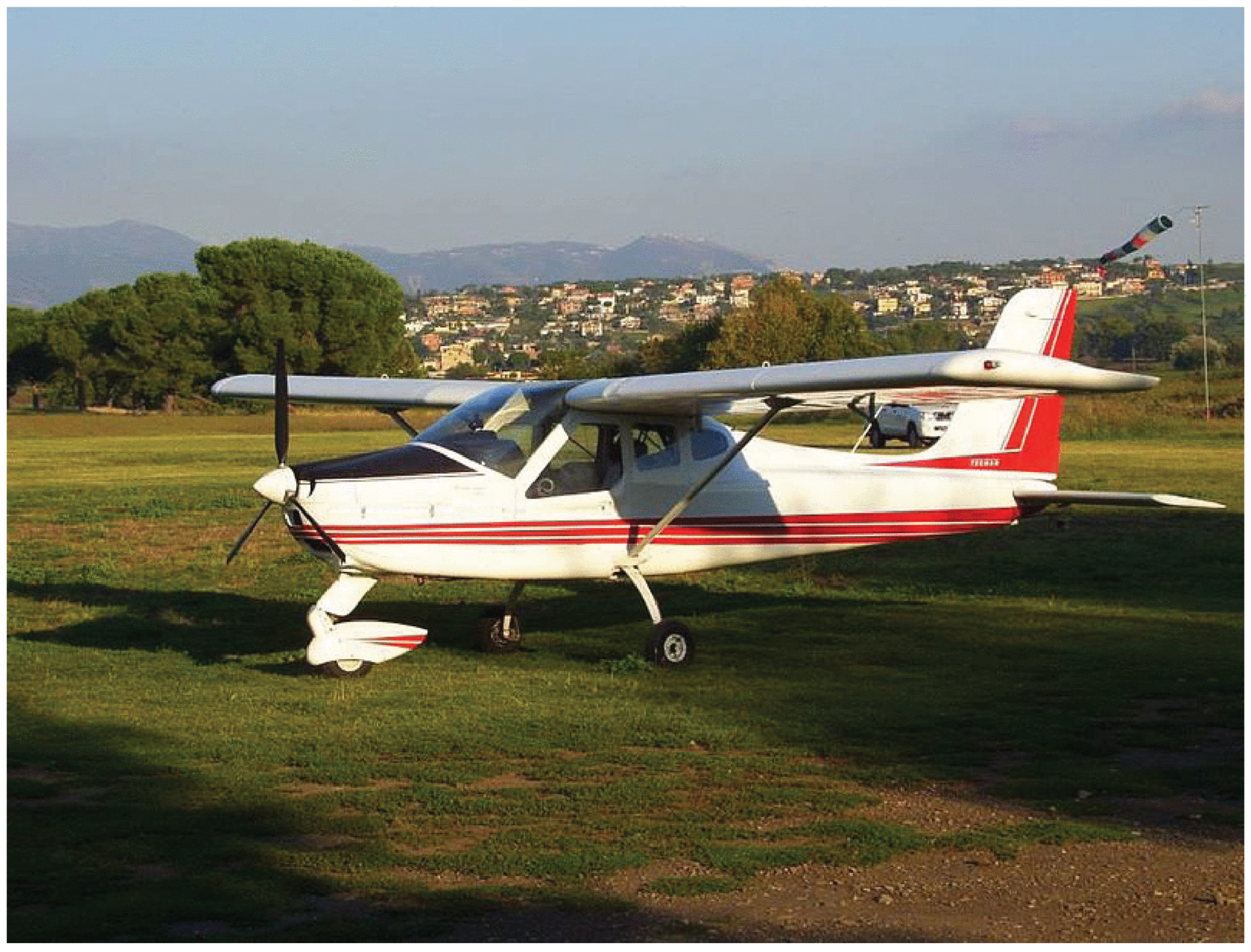
The considered FI and FE techniques were designed and validated using sensor flight data from a Tecnam P92 aircraft, shown in Figure 1. The aircraft mass is approximately 600 kg, and the propulsion is provided by a 74 kW Rotax 912 ULS with a two-blade fixed-pitch propeller, for a maximum cruise speed of 219 km/h and an operational ceiling of 4200 m. Data were acquired in semi-autonomous mode; in other words, the aircraft was manually flown by a pilot during the take-off and landing phase, while flown autonomously in cruise flight conditions. A set of nine flight datasets was considered in this study, of which five flights (with a total length of 2 h and 20 min) were used for the design of the FI and FE schemes, while the remaining four (with a total length of 2 h and 5 min) were used for validation purposes. These proprietary flight data previously acquired as part of an internal industrial research study for aircraft certification purposes were provided courtesy of Tecnam corporation. The data sampling time was set at 0.1 s. The study did not consider data associated with take-off, initial climb, final descent, and landing phases for the specific reason that in those flight conditions, the aerodynamic behavior of the aircraft is quite different with respect to cruise conditions due to the deployment of flaps. The use of multi-flight data for the training and the validation tasks is extremely important because, as for all data-driven techniques, the reliability of the results strongly depends on the completeness of the data, their spectral richness, and the coverage of all operating conditions. A total of 20 sensors was considered in this study, and they are listed in Table 2. The FI schemes were designed for the set of the 14 sensors indicated in Table 2 (the signals in (3), while the six actuation signals were the control deflections and engine commands (the signals in (3).
Data Normalization
The experimental data listed in Table 2 have quite different ranges and orders of magnitude; this issue suggested using a data normalization to zero mean and unit standard deviation.
The presence of regressor signals with very different operative ranges could cause the exclusion of the informative regressors with lower power from the model. This problem is avoided through normalization, which makes all signals with zero mean and unit variance. For each a signal, the normalization was performed using:
where is the i-th non-normalized signal ( or ); is its mean, and is its standard deviation. Since the signals are normalized, this implies that faults in (8) are associated with normalized signals; therefore, the fault amplitude estimations provided by (19), (23), (37) and (39) must be de-normalized to recover the actual fault amplitude. This can be achieved inverting (44), so that, assuming to be the normalized fault reconstructed through (19), (23), (37) and (39), the actual amplitude of the fault is:
7. Experimental Models for Sensor FI
The fault isolation techniques introduced in Section 3 and Section 4 require the definition of linear multivariate models. Specifically, the definition of the matrices and associated with the linear models in (4) is required. For each one of the sensors, the model was identified separately using standard system identification techniques [3]. From (3), the resulting models are:
where and are the i-th row of the matrices and , respectively. Each of these 14 models depends on 20 potential regressors. It is common practice in model identification to select a subset of regressors that are critical for the estimation of the predicted output . The regressors’ selection step was partially automated using the algorithm known as the “stepwise regressor selection method”. This is a well-known iterative data-driven algorithm for implementing a linear model by successively adding and/or removing regressors based on their statistical significance in a regression model [60]. In this effort, the stepwise selection was based on the training data using the ad-hoc procedure available in [61]. For each model, the selection of the best set of regressors was formulated through the analysis of the Root Mean Squared Error (RMSE) of the prediction error defined as:
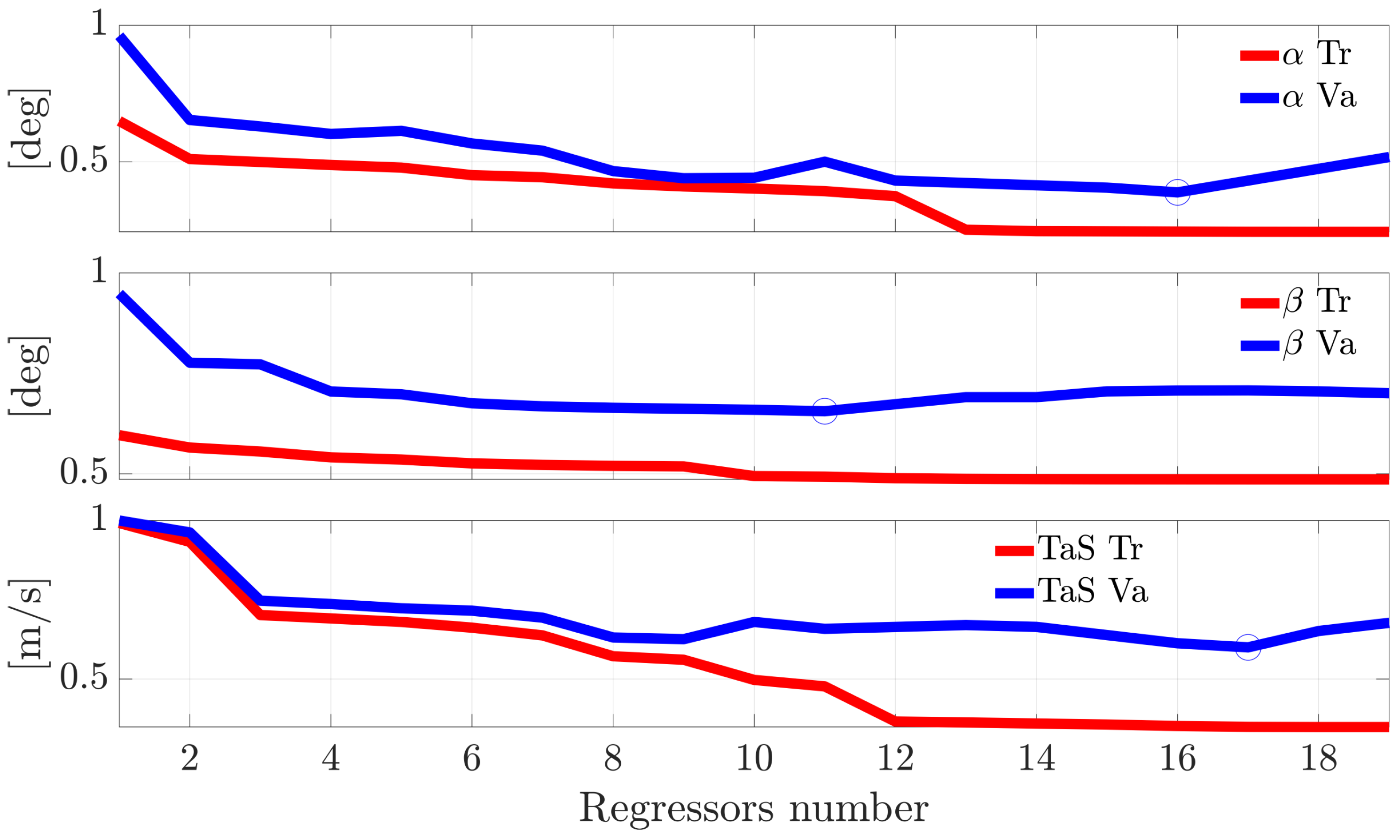
Figure 2 shows the evolution of the RMSE for the models of the sensors , , and evaluated both on the training and the validation flight data as a function of the number of regressors included in the model. As expected, while the training data result in a monotone decrease of the RMSE with the increase of the number of regressors in the model, for the validation data, the RMSE reaches a minimum; also, a larger number of regressors induces a decrease of the prediction accuracy. This is a typical example of the well-known modeling overfitting problem. Consequently, for each sensor, the best model was identified as the one that produced the minimum RMSE on the validation data set. The sets of regressors selected by this approach for the , , and models are reported in Table 3. Without any loss of generality, this procedure was also applied to the other remaining 11 sensors. The number of regressors selected for the 14 models is reported in Table 4.
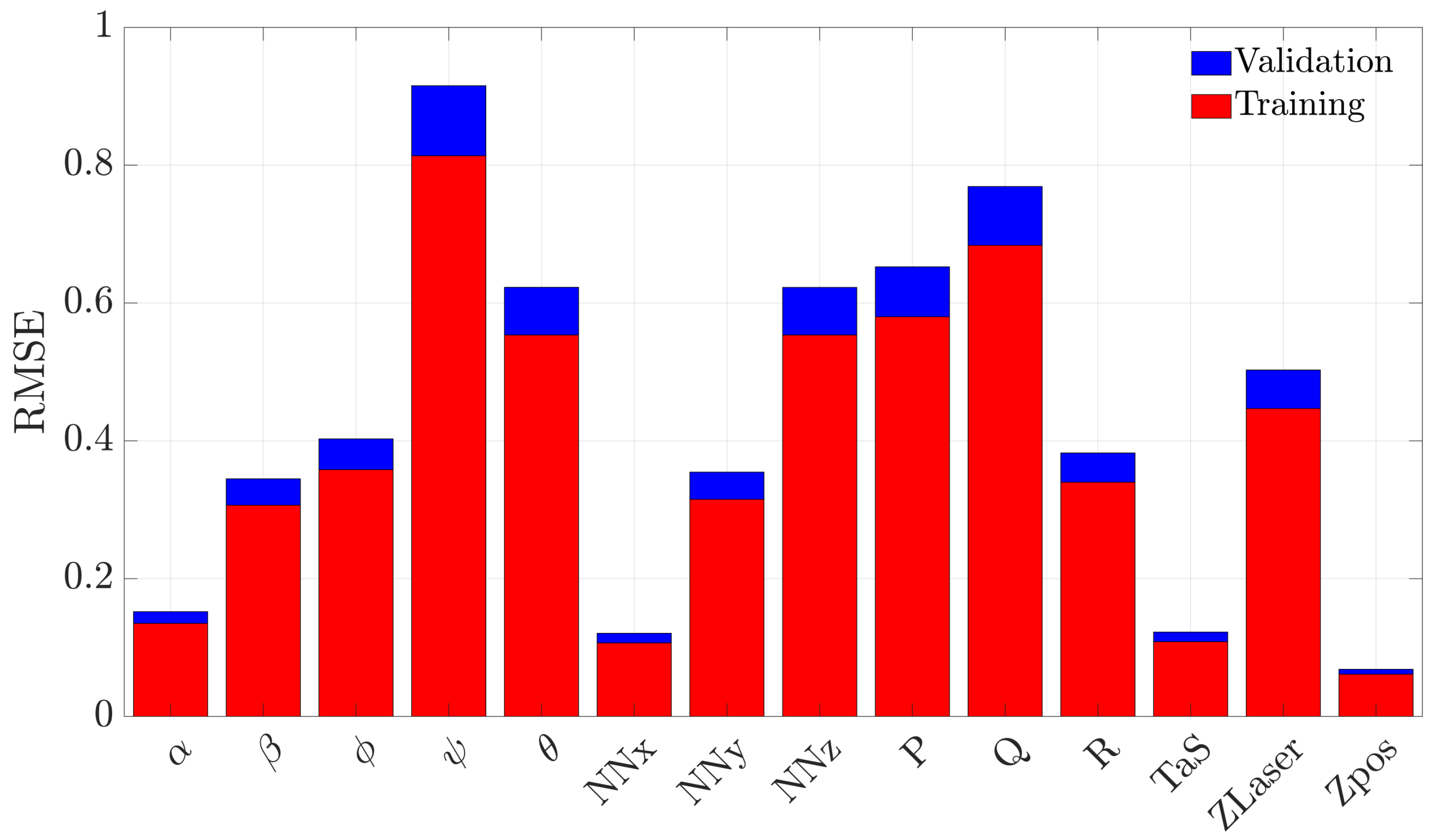
Figure 3 compares the RMSE for the 14 models produced by the (normalized) training and validation flight data. It is observed, for all models, that the training and the validation performance are comparable; this implies that the adopted regressor selection procedure is substantially correct and successfully avoids overfitting problems.
8. FI and FE Performance on the Validation Data (Offline Analysis)
For brevity purposes, only the results of the analysis relative to the air data sensors , , and are reported. However, it should be emphasized that the implemented schemes consider the entire set of sensors (residuals); in other words, the FI schemes isolate one among the 14 sensors.
Further, since the main purpose of this research is to compare the performance of the FI and FE techniques, the following analysis was performed assuming an “ideal” failure detection, i.e., the occurrence of a fault is detected as soon as it is injected into a generic time instant . Clearly, in practice, fault detection is not instantaneous, and a fault detection delay is to be expected before the FI and FE algorithms are activated.
The overall evaluation of the FI and FE of the schemes was performed evaluating the average performance provided by the set of four validation flights (approximately 2.05 h) by injecting the faults in the first sample of each validation flight (). The analysis was then performed considering, for each sensor, 50 equally-spaced fault amplitudes in (9) in the range [; ]. The maximum amplitudes (see Table 5) were selected empirically so that, for , the FI algorithms correctly isolate the fault with a percentage greater than (see Section 8.1).
The performance was analyzed using two specific metrics, that is the Fault Isolation Percentage (FIP) and the Relative Fault Reconstruction Error (RFRE). Both metrics are described below.
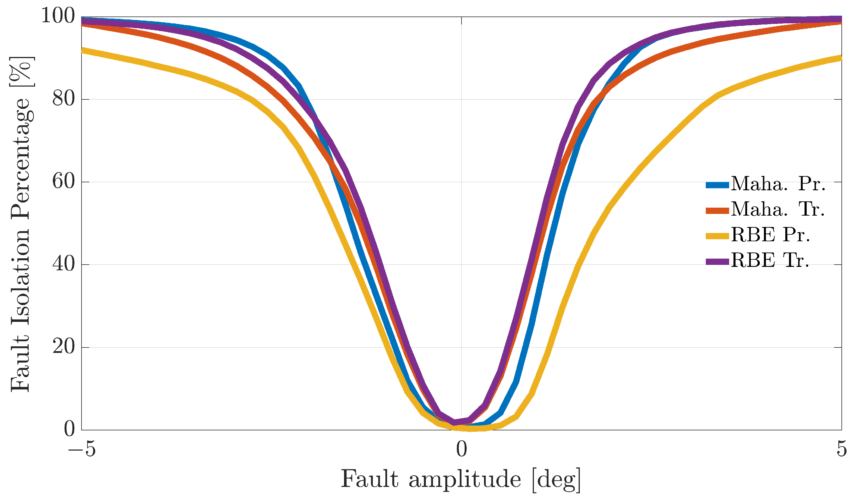
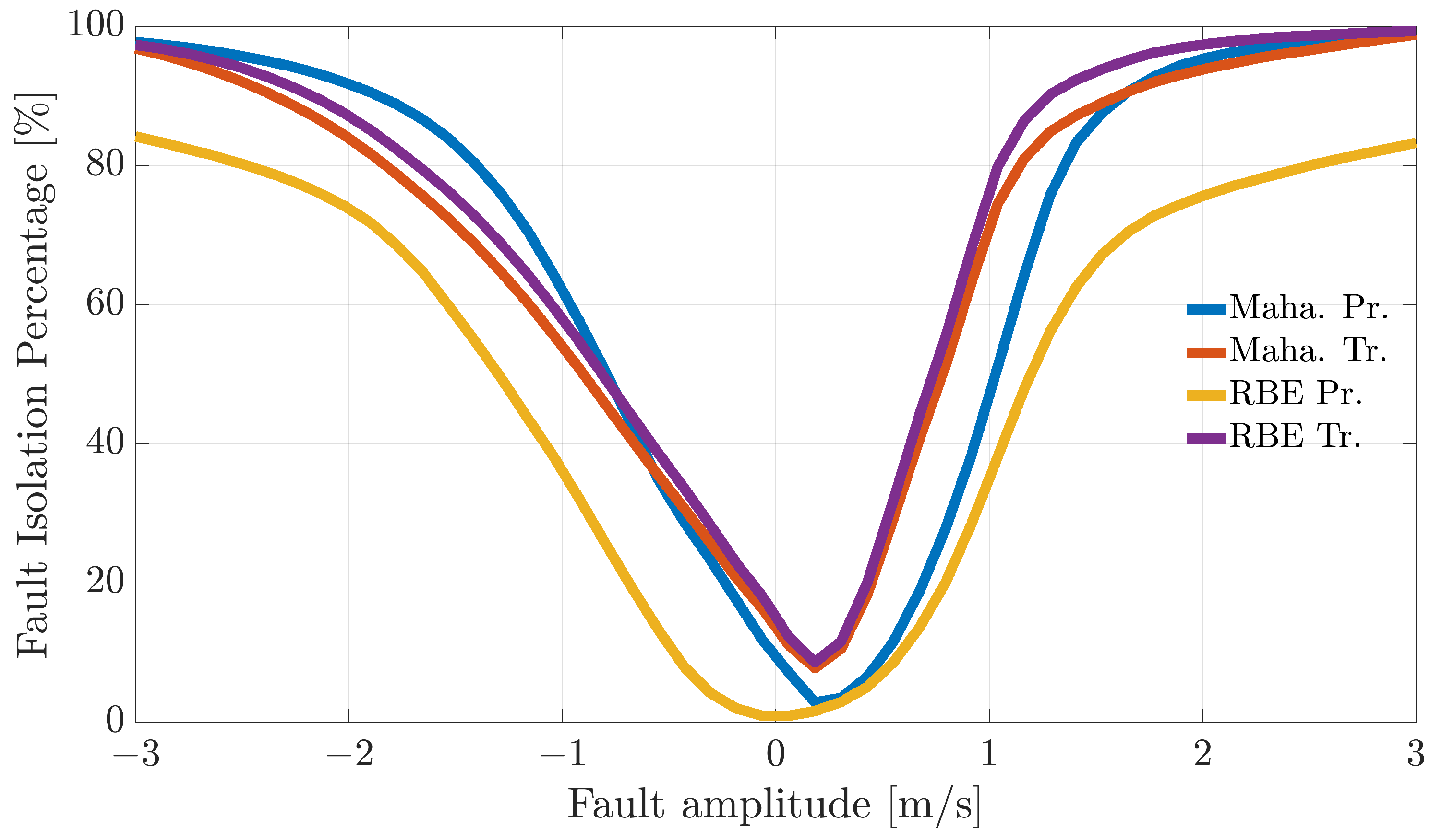
8.1. Fault Isolation Percentage
Considering a fault on the i-th sensor of amplitude in the j-th validation flight, the Fault Isolation Percentage (FIP) denoted by is defined as the percent ratio over all the validation flights between the number of samples for which the fault is correctly attributed to the i-th sensor and the total number of samples:
where:
- : number of validation flights.
- : number of samples for which the fault isolation index correctly isolates the fault on the i-th sensor, in validation flight j, for fault amplitude .
- : total number of samples in validation flight j.
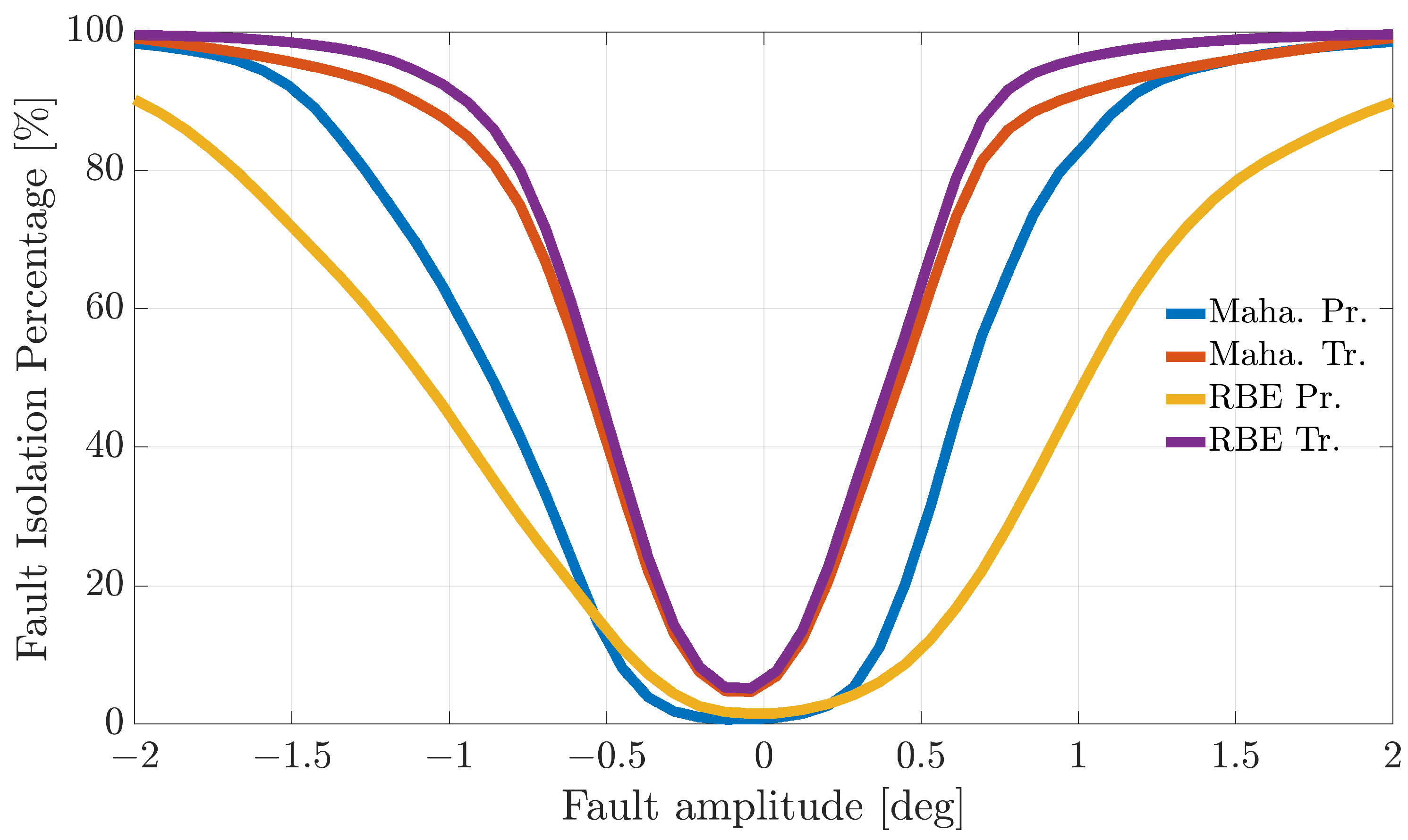
Figure 4, Figure 5 and Figure 6 show the FIP for the three sensors as a function of the fault amplitude computed using the validation flights for each of the considered techniques.
The analysis of the plots reveals that all the techniques can guarantee 100% correct fault isolation for large enough fault amplitudes for all the sensors. On the other side, small amplitude faults are often misinterpreted and misclassified. This is not surprising since small-amplitude faults have amplitudes similar to those of modeling errors, making the FI unreliable. The techniques Maha-Trand RBE-Tr based on transformed residuals provide better performance compared to the techniques based on primary residuals. This highlights the fact that the residual transformation based on the diagonalization of the noise covariance matrix is effective at improving FI performance.
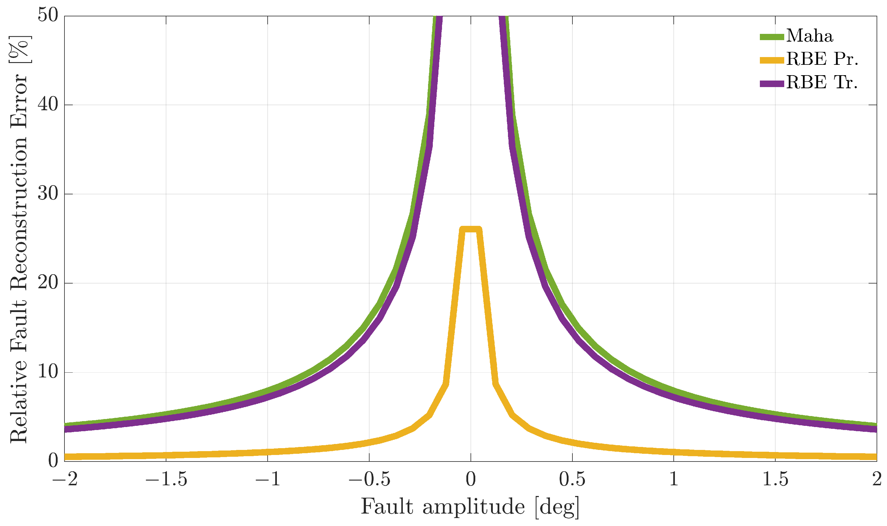
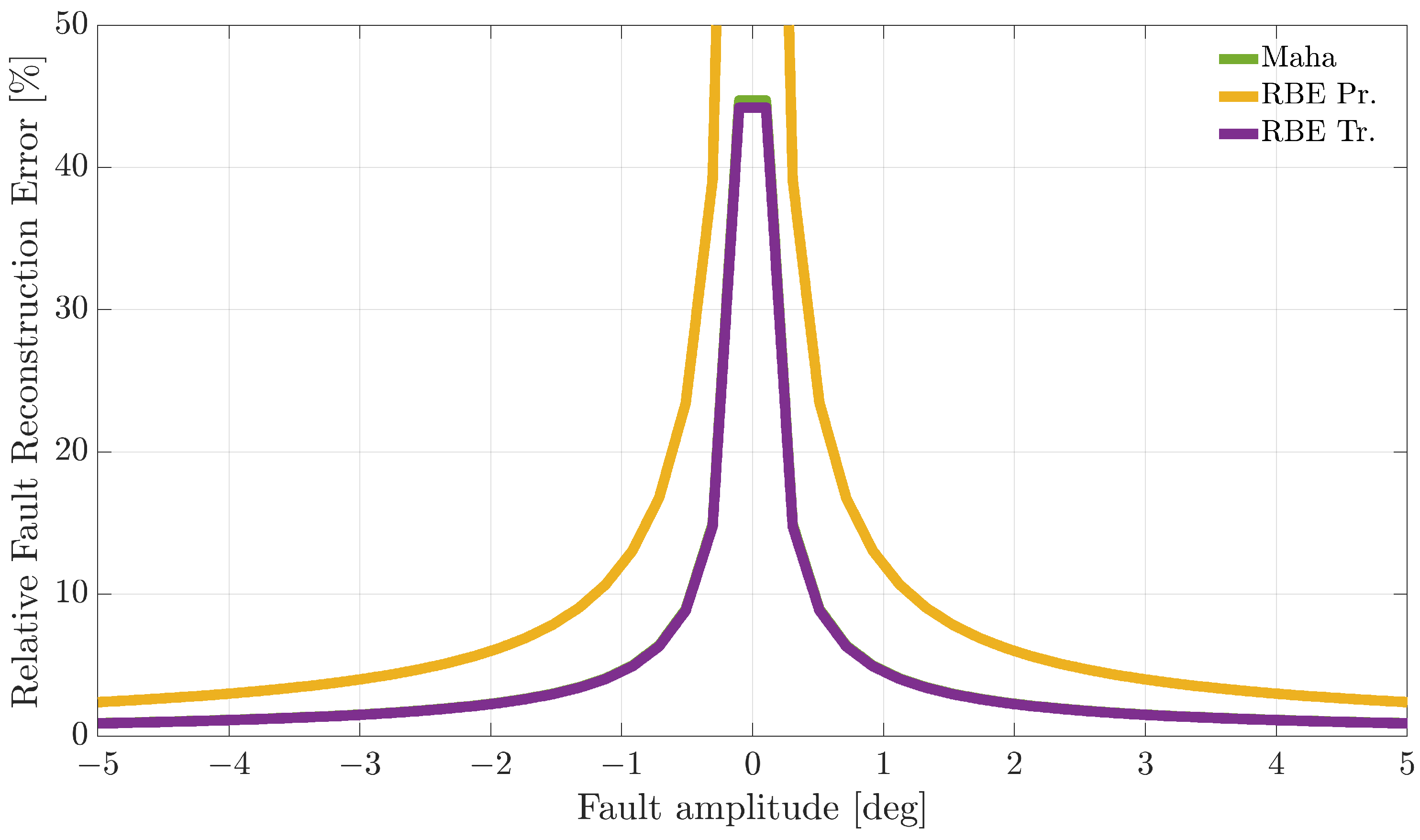
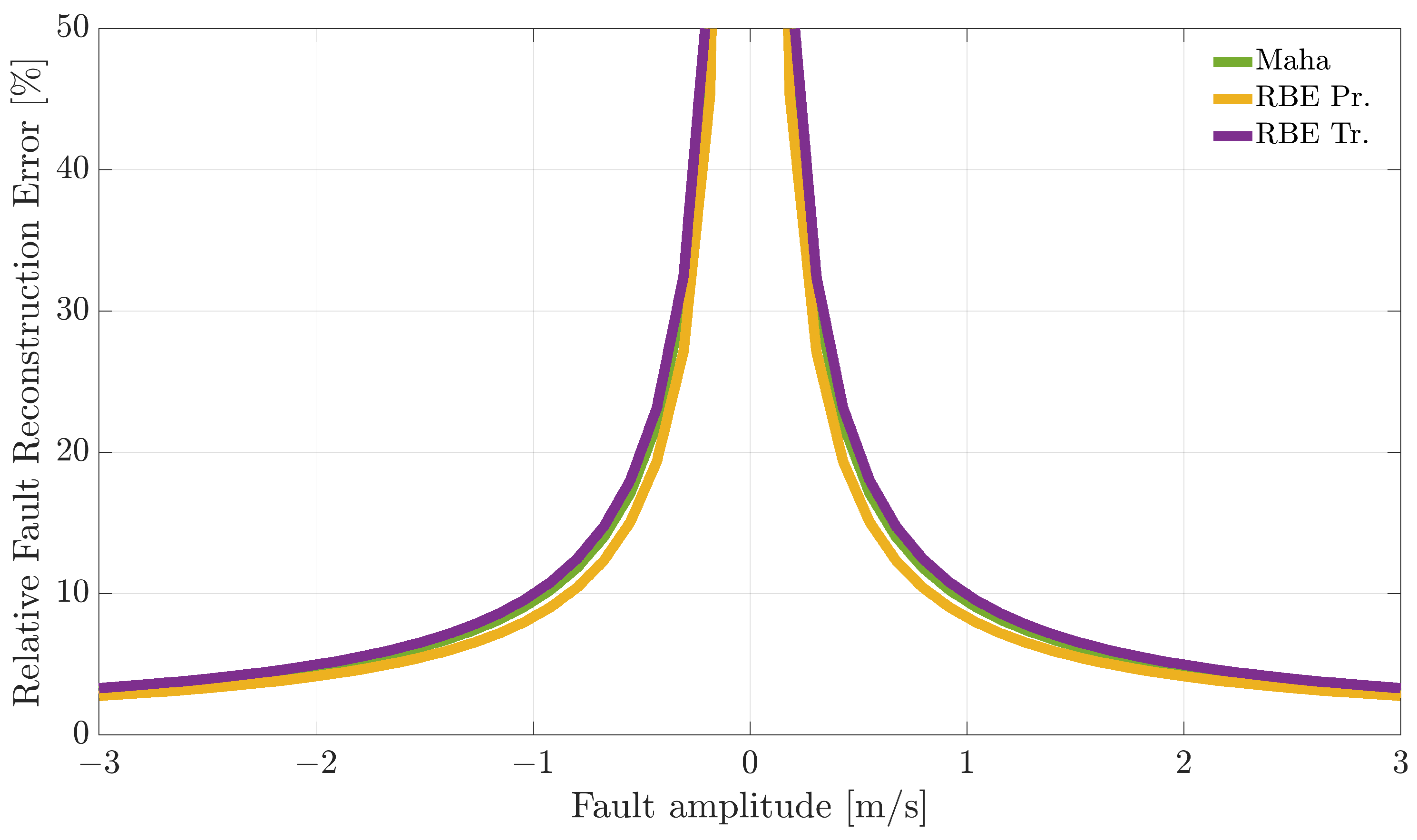
8.2. Relative Fault Reconstruction Error
Considering a fault on the i-th sensor of amplitude in the j-th validation flight, the Relative Fault Reconstruction Error (RFRE) is defined as the percent mean relative amplitude reconstruction error, that is:
where:
- : amplitude of the fault on sensor i;
- : amplitude of the reconstructed fault at sample time k for the validation flight j.
- : set of samples in validation flight j where the fault is correctly attributed to the i-th sensor.
- : number of samples in the set .
Figure 7, Figure 8 and Figure 9 compare the RFRE as a function of the fault amplitude. From the analysis of the figures, it can be observed that all the techniques accurately estimate the amplitude of either positive or negative faults for a large enough fault amplitude; instead, the estimate is not accurate for small amplitude faults. This is not surprising since when the amplitude of the fault has a magnitude of the same order as the estimator modeling error, the relative fault reconstruction is unreliable and inaccurate. For the index, it is not possible to identify a clear winning approach. Indeed, the RBE-Pr method provided the best results for the sensor, the worst for the sensor, while for the sensor, the performance was comparable.
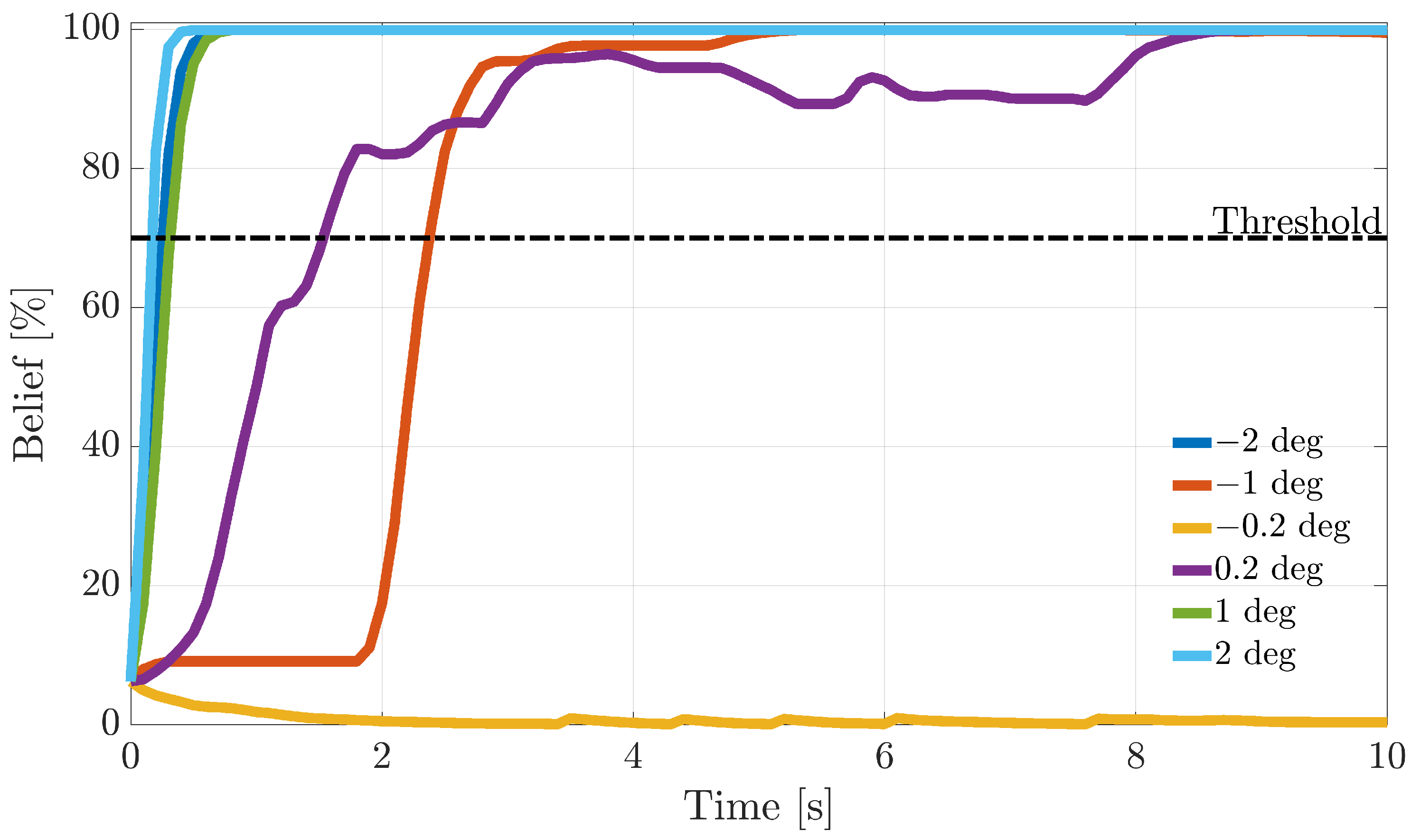
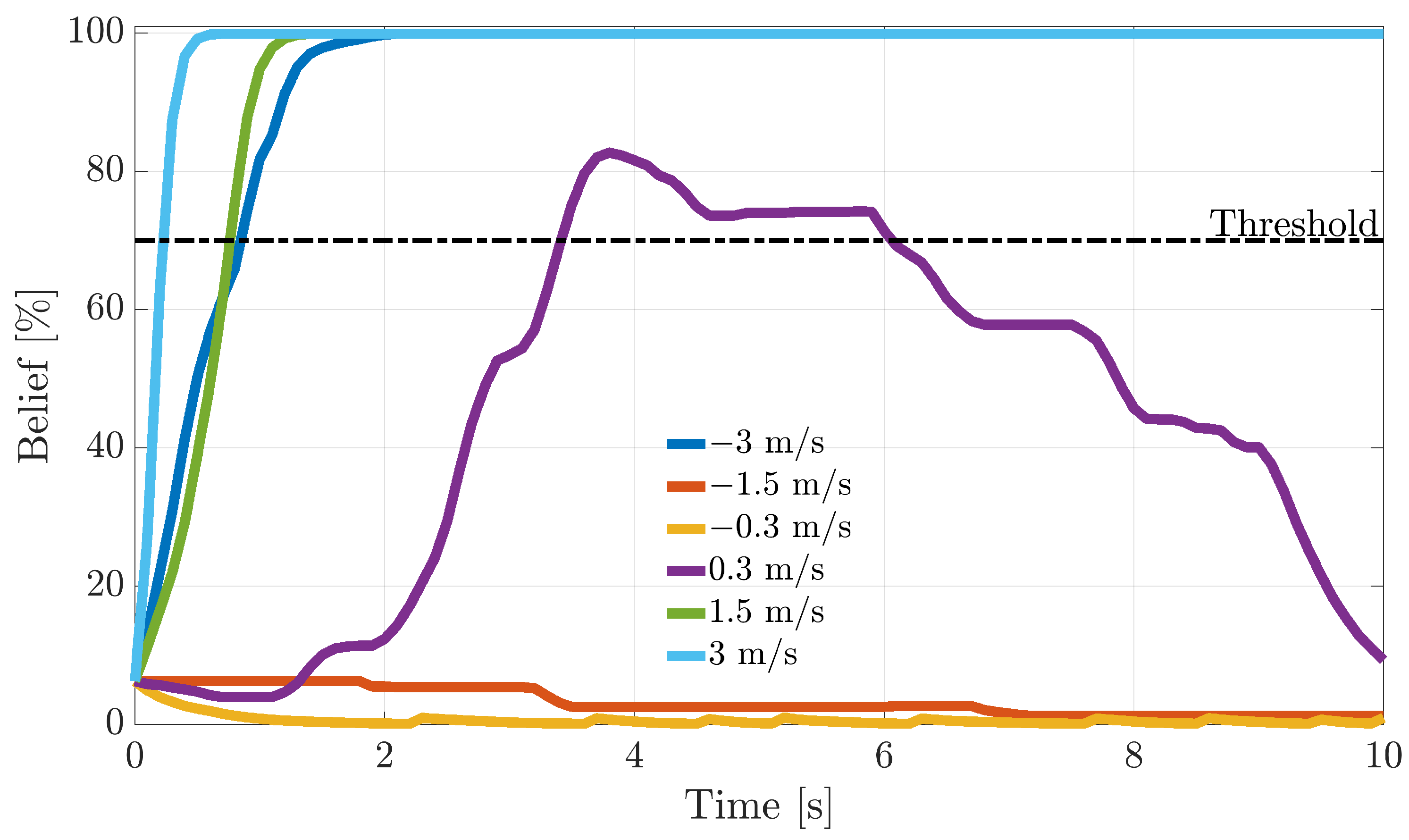
9. FI Performance on Validation Data (Online Analysis)
During the flight, following fault detection, it is critical to quickly isolate the faulty sensors and, next, to take the appropriate reconfiguration actions. In this section, the dynamic response of FI methods based on the recursive BFs introduced in Section 5 is analyzed. To understand the online operation in Figure 10, Figure 11 and Figure 12, the evolution of the fault beliefs ( in (40) for the RBE-Pr technique for a fault injected at equal to 50% of the duration of a validation flight is shown. In the figures, the results for fault amplitudes equal to , , and ± sample-variance of the residuals in fault fault-free conditions are provided.
It is observed that the fault beliefs grow monotonically for large and intermediate fault amplitudes, reaching in a short time the “fault declaration threshold” (set to 70%) when a fault on the i-th sensor is declared. On the other side, for a fault amplitude equal to ± the sample variance of the modeling error, the fault beliefs in most cases are not strong enough to reach the threshold; thus, the fault cannot be isolated.
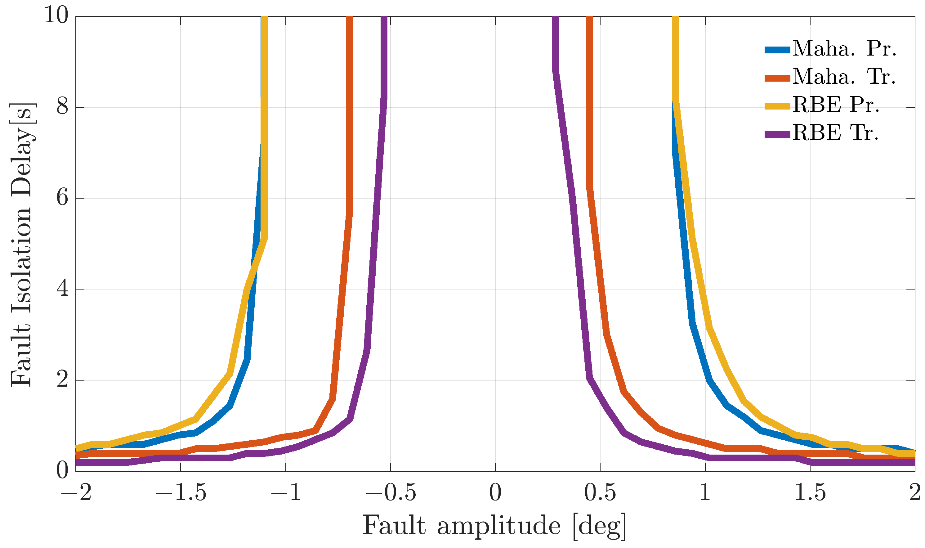
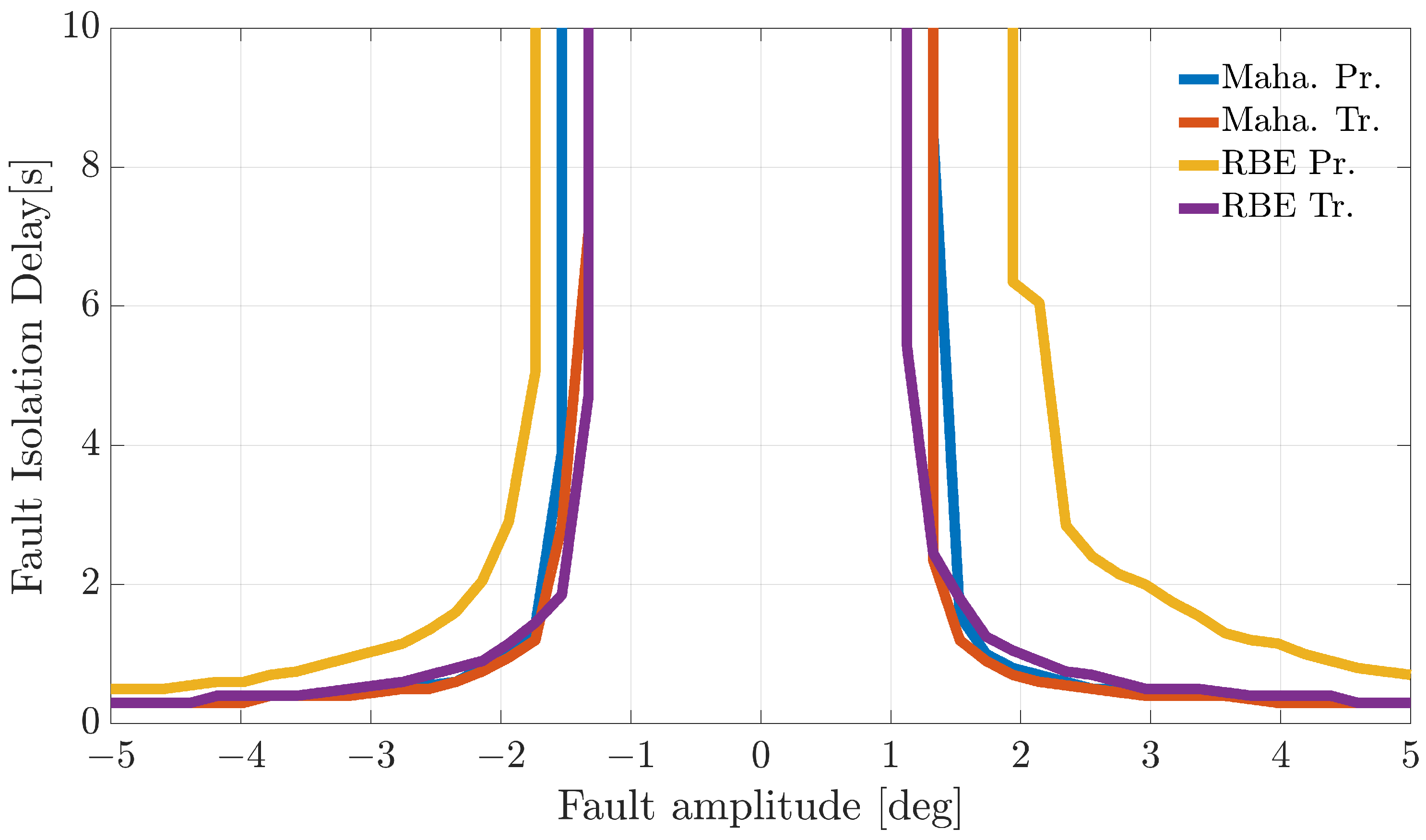
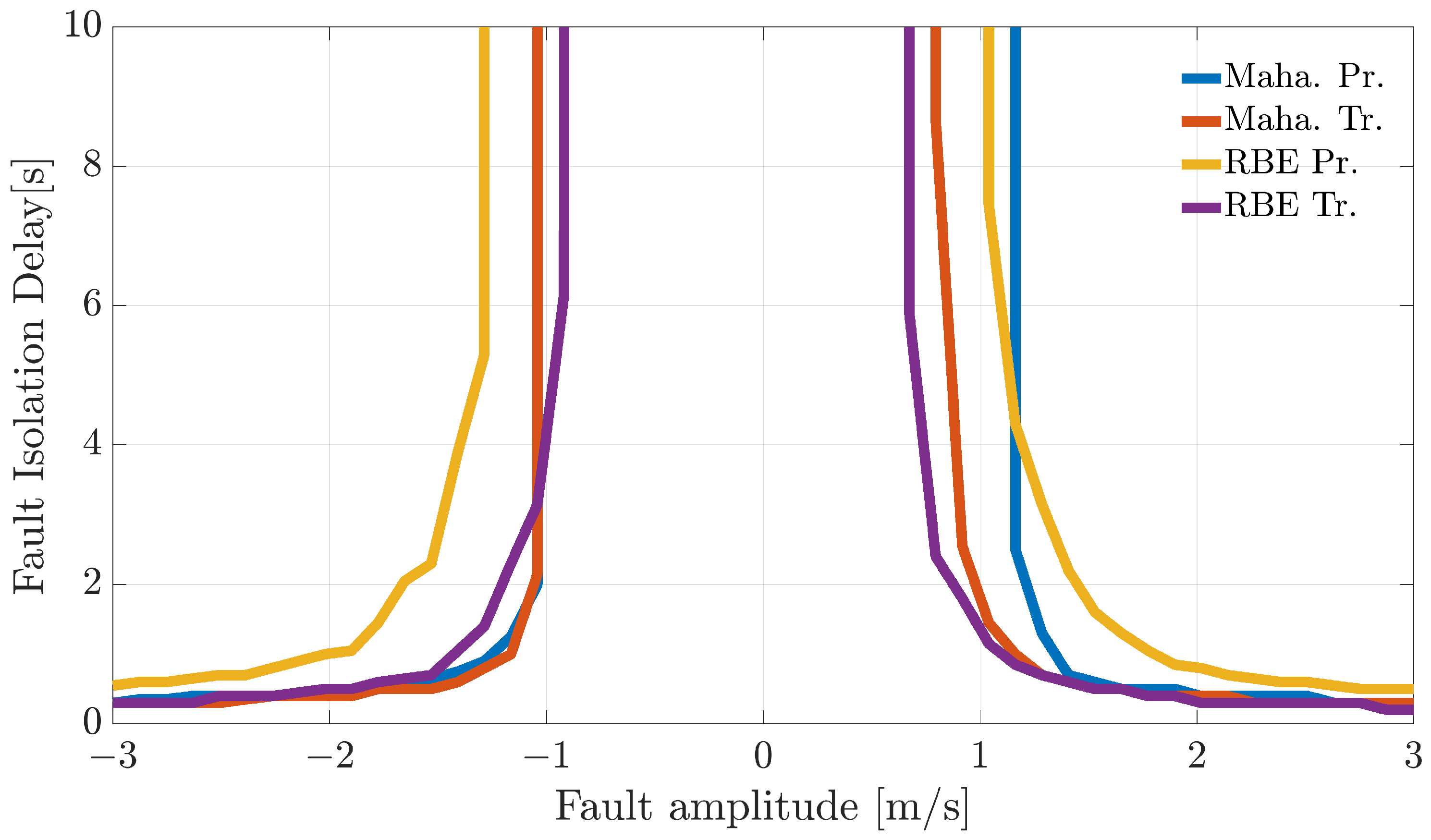
Fault Isolation Delay
Fault isolation delay quantifies the (mean) time delay between the generic FD and the instant the FI algorithm reaches, for the first time, a fault belief equal to the predefined “fault declaration threshold”. As highlighted in Figure 10, Figure 11 and Figure 12, this delay depends mainly on the fault amplitude, but may depend also on the in-flight fault instant. To evaluate the online FI performance of the schemes, faults (9) were injected into 10 equally-spaced time instants for each validation flight. For a fault amplitude on the i-th sensor, the (mean) fault isolation delay is defined as:
where:
- : for a validation flight j and for a fault amplitude , denotes the time from the injection of the fault at and the time for which the belief associated with the i-th sensor reaches for the first time the threshold.
- : set of equally-spaced instants () in the validation flight j when the fault (9) is injected in the i-th sensor.
- : number of samples in the set .
Figure 13, Figure 14 and Figure 15 show the index (50) as a function of the fault amplitude. For small-amplitude faults, in case the fault is not isolated within an observation window of 10 s, the corresponding fault isolation time is conventionally set to a very large value. Analyzing the figures, it can be observed that Bayesian filtering for all the methods guarantees a reliable declaration of medium-large faults within 3–4 s. For all three sensors, the best performance (smaller ) was provided by the RBE-Tr. method. Performance degraded quickly for all the methods in the case of small amplitude faults since, in some cases, the fault belief does not reach the fault declaration thresholds within the allowed observation window. Furthermore, in this case, the experimental results confirm that techniques based on transformed directional residuals are more effective (lower mean fault isolation delay) than techniques based on primary directional residuals.
10. Conclusions
The purpose of this effort was to compare well-known analytical redundancy-based data-driven techniques for the Fault Isolation (FI) and Fault Estimation (FE) of a set of 14 sensors of a semi-autonomous aircraft. While all these techniques have been shown in the literature to provide close to perfect results using simulated data, only the use of actual experimental data provides the necessary insights and understanding leading to the selection of the best approaches. Specifically, multiple sets of flight data were used to identify linear multivariate models providing a set of primary residuals. Then, residual transformation techniques were applied to generate directional residuals that are robust with respect to the modeling errors. Next, Mahalanobis distance and reconstruction-based methods were used for the FI and the FE. Detailed tests (performed on a set of four validation flights) on the air data sensors showed that the reconstruction-based techniques featuring transformed residuals provide better performance compared to the primary residual-based techniques in terms of the overall fault isolation percentage and fault reconstruction accuracy indices.
In-flight FI was also investigated by applying a bank of recursive Bayesian filters to manage the directional error information online from the 14 sensors. A detailed analysis was conducted by injecting variable amplitude faults at different points throughout the flights. This allowed the estimation of the mean in-flight fault isolation delay. Even for this case, the reconstruction-based methods relying on transformed residuals provided the best performance.
All the considered FI and FE methods are data-driven and were designed based on actual flight data. Therefore, the schemes do not require a priori knowledge of detailed aircraft modeling for their implementation and can be easily returned regularly with updated flight data. Although this is undoubtedly a useful aspect, it is also worth noting, as for any data-based technique, that the reliability of the results depends heavily on the completeness of the available data, which must be representative of all operating conditions. In order to address this issue, all our models were derived by taking multi-flight data rich in maneuvers (as opposed to cruise steady-state conditions), both in the design and validation phases. The quantitative results provide a clear picture of the requested design effort as far as the achievable performance using well-known FI and FE schemes.
Author Contributions
Conceptualization, N.C., M.R.N. and M.L.F.; methodology, M.R.N. and M.L.F.; software, N.C.; validation, N.C.; formal analysis, N.C.; investigation, N.C. and G.C.; resources, M.L.F.; data curation, M.R.N. and M.L.F.; writing—original draft preparation, N.C.; writing—review and editing, M.R.N. and M.L.F.; visualization, N.C. and G.C.; supervision, M.R.N. and M.L.F.; project administration, M.L.F.; funding acquisition, G.C. and M.L.F. All authors have read and agreed to the published version of the manuscript.
Funding
This research was partially supported by the University of Perugia through the 2017 and 2018 Basic Research Funds (Projects: RICBA17MR and RICBA18MR).
Acknowledgments
The authors would like to thank Giuseppe Del Core for providing the P92 Tecnam flight data.
Conflicts of Interest
The authors declare that there are no conflicts of interest in performing this research.
Abbreviations
The following abbreviations are used in this manuscript:
| Maha. Pr. | Mahalanobis distance-based technique with Primary residuals |
| Maha. Tr. | Mahalanobis distance-based technique with Transformed residuals |
| RBE Pr. | Reconstruction-based technique with Primary residuals |
| RBE Tr. | Reconstruction-based technique with Transformed residuals |
References
- Ding, S. Model-Based Fault Diagnosis Techniques: Design Schemes, Algorithms, and Tools; Springer: Berlin/Heidelberg, Germany, 2008. [Google Scholar] [CrossRef]
- Gertler, J. Analytical Redundancy Methods in Fault Detection and Isolation-Survey and Synthesis. IFAC Proc. Vol. 1991, 24, 9–21. [Google Scholar] [CrossRef]
- Simani, S.; Fantuzzi, C.; Patton, R. Model-Based Fault Diagnosis in Dynamic Systems Using Identification Techniques; Springer: Berlin/Heidelberg, Germany, 2003. [Google Scholar] [CrossRef] [Green Version]
- Isermann, R. Process fault detection based on modeling and estimation methods—A survey. Automatica 1984, 20, 387–404. [Google Scholar] [CrossRef]
- Basseville, M. Detecting changes in signals and systems—A survey. Automatica 1988, 24, 309–326. [Google Scholar] [CrossRef]
- Gertler, J. Fault Detection and Diagnosis in Engineering Systems; Routledge: London, UK, 2017. [Google Scholar]
- Patton, R.J.; Frank, P.M.; Clark, R.N. Issues of Fault Diagnosis for Dynamic Systems; Springer Science & Business Media: Berlin/Heidelberg, Germany, 2013. [Google Scholar]
- Gao, Z.; Cecati, C.; Ding, S.X. A Survey of Fault Diagnosis and Fault-Tolerant Techniques—Part I: Fault Diagnosis with Model-Based and Signal-Based Approaches. IEEE Trans. Ind. Electron. 2015, 62, 3757–3767. [Google Scholar] [CrossRef] [Green Version]
- Blanke, M.; Kinnaert, M.; Lunze, J.; Staroswiecki, M. Diagnosis and Fault Tolerant Control; Springer: Berlin/Heidelberg, Germany, 2016. [Google Scholar]
- Ding, S. Optimal fault detection and estimation: A unified scheme and least squares solutions. IFAC-PapersOnLine 2018, 51, 465–472. [Google Scholar] [CrossRef]
- Li, L.; Ding, S.; Peng, X. Optimal Observer-based Fault Detection and Estimation Approaches for T-S Fuzzy Systems. IEEE Trans. Fuzzy Syst. 2020. [Google Scholar] [CrossRef]
- Martinez-Guerra, R.; Mata-Machuca, J.L. Fault Detection and Diagnosis in Nonlinear Systems; Springer: Berlin/Heidelberg, Germany, 2016. [Google Scholar]
- Sobhani-Tehrani, E.; Khorasani, K. Fault Diagnosis of Nonlinear Systems Using a Hybrid Approach; Springer Science & Business Media: Berlin/Heidelberg, Germany, 2009; Volume 383. [Google Scholar]
- Zhang, Q.; Zhang, X.; Polycarpou, M.M.; Parisini, T. Distributed sensor fault detection and isolation for multimachine power systems. Int. J. Robust Nonlinear Control 2014, 24, 1403–1430. [Google Scholar] [CrossRef]
- Isermann, R. Model-based fault-detection and diagnosis—Status and applications. Annu. Rev. Control 2005, 29, 71–85. [Google Scholar] [CrossRef]
- Ding, S. Data-Driven Design of Fault Diagnosis and Fault-Tolerant Control Systems; Springer: Berlin/Heidelberg, Germany, 2014. [Google Scholar] [CrossRef]
- Yin, S.; Ding, S.X.; Haghani, A.; Hao, H.; Zhang, P. A comparison study of basic data-driven fault diagnosis and process monitoring methods on the benchmark Tennessee Eastman process. J. Process Control 2012, 22, 1567–1581. [Google Scholar] [CrossRef]
- Mrugalski, M. Advanced Neural Network-Based Computational Schemes for Robust Fault Diagnosis; Springer: Berlin/Heidelberg, Germany, 2014. [Google Scholar]
- Bocaniala, C.D.; Palade, V. Computational intelligence methodologies in fault diagnosis: Review and state of the art. In Computational Intelligence in Fault Diagnosis; Springer: Berlin/Heidelberg, Germany, 2006; pp. 1–36. [Google Scholar]
- Lei, Y.; Yang, B.; Jiang, X.; Jia, F.; Li, N.; Nandi, A.K. Applications of machine learning to machine fault diagnosis: A review and roadmap. Mech. Syst. Signal Process. 2020, 138, 106587. [Google Scholar] [CrossRef]
- López-Estrada, F.R.; Méndez López, L.; Santos-Ruiz, I.; Valencia-Palomo, G. Detección de fallas en vehículos aéreos no tripulados mediante señales de orientación y técnicas de aprendizaje de máquina. Revista Iberoamericana de Automática e Informática Industrial RIAI 2021. [Google Scholar] [CrossRef]
- Schaefer, R. Unmanned Aerial Vehicle Reliability Study; Office of the Secretary of Defense: Washington, DC, USA, 2003. [Google Scholar]
- Goupil, P. AIRBUS state of the art and practices on FDI and FTC in flight control system. Control Eng. Pract. 2011, 19, 524–539. [Google Scholar] [CrossRef]
- Johnson, D.M. A review of fault management techniques used in safety-critical avionic systems. Prog. Aerosp. Sci. 1996, 32, 415–431. [Google Scholar] [CrossRef]
- Marzat, J.; Piet-Lahanier, H.; Damongeot, F.; Walter, E. Model-based fault diagnosis for aerospace systems: A survey. Proc. Inst. Mech. Eng. Part G J. Aerosp. Eng. 2012, 226, 1329–1360. [Google Scholar] [CrossRef] [Green Version]
- Farsoni, S.; Simani, S. Robust Fault Diagnosis and Fault Tolerant Control of Wind Turbines: Data-Driven and Model-Based Approaches; Scholars’ Press: Riga, Latvia, 2016. [Google Scholar]
- Chu, E.; Gorinevsky, D.; Boyd, S. Detecting Aircraft Performance Anomalies from Cruise Flight Data; AIAA Infotech@Aerospace: Atlanta, Georgia, 2010. [Google Scholar] [CrossRef] [Green Version]
- Li, L.; Gariel, M.; Hansman, R.J.; Palacios, R. Anomaly detection in onboard-recorded flight data using cluster analysis. In Proceedings of the 2011 IEEE/AIAA 30th Digital Avionics Systems Conference, Seattle, WA, USA, 16–20 October 2011; pp. 4A4-1–4A4-11. [Google Scholar] [CrossRef]
- Dani, M.C.; Freixo, C.; Jollois, F.; Nadif, M. Unsupervised anomaly detection for Aircraft Condition Monitoring System. In Proceedings of the 2015 IEEE Aerospace Conference, Big Sky, MT, USA, 7–14 March 2015; pp. 1–7. [Google Scholar] [CrossRef]
- Li, L.; Das, S.; John Hansman, R.; Palacios, R.; Srivastava, A.N. Analysis of Flight Data Using Clustering Techniques for Detecting Abnormal Operations. J. Aerosp. Inf. Syst. 2015, 12, 587–598. [Google Scholar] [CrossRef] [Green Version]
- Lu, P.; Van Eykeren, L.; van Kampen, E.J.; de Visser, C.; Chu, Q. Double-model adaptive fault detection and diagnosis applied to real flight data. Control Eng. Pract. 2015, 36, 39–57. [Google Scholar] [CrossRef]
- Fravolini, M.L.; Napolitano, M.R.; Core, G.D.; Papa, U. Experimental interval models for the robust Fault Detection of Aircraft Air Data Sensors. Control Eng. Pract. 2018, 78, 196–212. [Google Scholar] [CrossRef]
- Fravolini, M.L.; Del Core, G.; Papa, U.; Valigi, P.; Napolitano, M.R. Data-Driven Schemes for Robust Fault Detection of Air Data System Sensors. IEEE Trans. Control Syst. Technol. 2019, 27, 234–248. [Google Scholar] [CrossRef]
- Tecnam P92 Webpage. 2020. Available online: https://www.tecnam.com/aircraft/p92-echo-mkii/ (accessed on 22 December 2020).
- Gertler, J.J.; Kunwer, M.M. Optimal residual decoupling for robust fault diagnosis. Int. J. Control 1995, 61, 395–421. [Google Scholar] [CrossRef]
- Basseville, M. Information criteria for residual generation and fault detection and isolation. Automatica 1997, 33, 783–803. [Google Scholar] [CrossRef] [Green Version]
- Hu, Y.; Gertler, J. Design of Directional Residuals for Optimal Testability. IFAC Proc. Vol. 2002, 35, 131–136. [Google Scholar] [CrossRef] [Green Version]
- Alcala, C.F.; Qin, S.J. Reconstruction-based contribution for process monitoring. Automatica 2009, 45, 1593–1600. [Google Scholar] [CrossRef]
- Frisk, E.; Nielsen, L. Robust residual generation for diagnosis including a reference model for residual behavior. Automatica 2006, 42, 437–445. [Google Scholar] [CrossRef] [Green Version]
- Varrier, S.; Koenig, D.; Martinez, J.J. Robust fault detection for Uncertain Unknown Inputs LPV system. Control Eng. Pract. 2014, 22, 125–134. [Google Scholar] [CrossRef] [Green Version]
- Witczak, M.; Buciakowski, M.; Puig, V.; Rotondo, D.; Nejjari, F. An LMI approach to robust fault estimation for a class of nonlinear systems. Int. J. Robust Nonlinear Control 2016, 26, 1530–1548. [Google Scholar] [CrossRef] [Green Version]
- Balzano, F.; Fravolini, M.; Napolitano, M.; d’Urso, S.; Crispoltoni, M.; Core, G. Air Data Sensor Fault Detection with an Augmented Floating Limiter. Int. J. Aerosp. Eng. 2018, 2018, 1072056. [Google Scholar] [CrossRef] [Green Version]
- Leondes, C.T. Techniques in Discrete and Continuous Robust Systems; Academic Press: Cambridge, MA, USA, 1996. [Google Scholar]
- Mahalanobis, P.C. On the generalized distance in statistics. Proc. Natl. Inst. Sci. 1936, 2, 49–55. [Google Scholar]
- De Maesschalck, R.; Jouan-Rimbaud, D.; Massart, D. The Mahalanobis distance. Chemom. Intell. Lab. Syst. 2000, 50, 1–18. [Google Scholar] [CrossRef]
- Qin, S.J. Survey on data-driven industrial process monitoring and diagnosis. Annu. Rev. Control 2012, 36, 220–234. [Google Scholar] [CrossRef]
- Cartocci, N.; Costante, G.; Napolitano, M.R.; Valigi, P.; Crocetti, F.; Fravolini, M.L. PCA Methods and Evidence Based Filtering for Robust Aircraft Sensor Fault Diagnosis. In Proceedings of the 2020 28th Mediterranean Conference on Control and Automation (MED), Saint-Raphaël, France, 16–19 June 2020; pp. 550–555. [Google Scholar] [CrossRef]
- Yang, F.; Xiao, D. Progress in Root Cause and Fault Propagation Analysis of Large-Scale Industrial Processes. J. Control Sci. Eng. 2012, 2012, 478373. [Google Scholar] [CrossRef]
- Massoumnia, M. A geometric approach to the synthesis of failure detection filters. IEEE Trans. Autom. Control 1986, 31, 839–846. [Google Scholar] [CrossRef]
- Hu, Y.; Gertler, J. Design of optimal directional residuals for linear dynamic systems. IFAC Proc. Vol. 2003, 36, 245–250. [Google Scholar] [CrossRef]
- Lou, X.C.; Willsky, A.S.; Verghese, G.C. Optimally robust redundancy relations for failure detection in uncertain systems. Automatica 1986, 22, 333–344. [Google Scholar] [CrossRef] [Green Version]
- Särkkä, S. Bayesian Filtering and Smoothing; Cambridge University Press: Cambridge, MA, USA, 2013; Volume 3. [Google Scholar]
- Bishop, C.M. Pattern Recognition and Machine Learning; Springer: Berlin/Heidelberg, Germany, 2006. [Google Scholar]
- Ge, Z.; Zhang, M.; Song, Z. Nonlinear process monitoring based on linear subspace and Bayesian inference. J. Process Control 2010, 20, 676–688. [Google Scholar] [CrossRef]
- Zheng, Y.; Mao, S.; Liu, S.; Wong, D.S.; Wang, Y. Normalized Relative RBC-Based Minimum Risk Bayesian Decision Approach for Fault Diagnosis of Industrial Process. IEEE Trans. Ind. Electron. 2016, 63, 7723–7732. [Google Scholar] [CrossRef]
- Zhu, J.; Ge, Z.; Song, Z. Distributed Parallel PCA for Modeling and Monitoring of Large-Scale Plant-Wide Processes with Big Data. IEEE Trans. Ind. Inform. 2017, 13, 1877–1885. [Google Scholar] [CrossRef]
- Zhou, W.; Yang, W.; Wang, Y.; Zhang, H. Generalized Reconstruction-Based Contribution for Multiple Faults Diagnosis with Bayesian Decision. In Proceedings of the 2018 IEEE 7th Data Driven Control and Learning Systems Conference (DDCLS), Enshi, China, 25–27 May 2018; pp. 813–818. [Google Scholar] [CrossRef]
- Basseville, M.; Nikiforov, I.V. Detection of Abrupt Changes—Theory and Application; Prentice Hall, Inc.: Upper Saddle River, NJ, USA, 1993; p. 550. [Google Scholar]
- Chandola, V.; Banerjee, A.; Kumar, V. Anomaly Detection: A Survey. ACM Comput. Surv. 2009, 41. [Google Scholar] [CrossRef]
- Draper, N.; Smith, H. Applied Regression Analysis, 3rd ed.; A Wiley-Interscience Publication; Wiley: New York, NY, USA, 1998. [Google Scholar]
- The Mathworks Inc. MATLAB—MathWorks; The Mathworks Inc.: Natick, MA, USA, 2020. [Google Scholar]
Figure 1.
The semi-autonomous Tecnam P92 aircraft.

Figure 2.
RMSE as function of the number of regressors in the model for the , , and sensors. Training (Tr) and Validation (Va) data.
Figure 2.
RMSE as function of the number of regressors in the model for the , , and sensors. Training (Tr) and Validation (Va) data.

Figure 3.
Comparison of the RMSE achieved in training and validation for the 14 linear regression models.
Figure 3.
Comparison of the RMSE achieved in training and validation for the 14 linear regression models.

Figure 4.
Fault isolation percentage for the sensor evaluated on the validation flights as a function of the fault amplitude.
Figure 4.
Fault isolation percentage for the sensor evaluated on the validation flights as a function of the fault amplitude.

Figure 5.
Fault isolation percentage for the sensor evaluated on the validation flights as a function of fault amplitude.
Figure 5.
Fault isolation percentage for the sensor evaluated on the validation flights as a function of fault amplitude.

Figure 6.
Fault isolation percentage for the sensor evaluated on the validation flights as a function of fault amplitude.
Figure 6.
Fault isolation percentage for the sensor evaluated on the validation flights as a function of fault amplitude.

Figure 7.
Relative fault reconstruction error for the sensor evaluated on the validation flights as a function of fault amplitude.
Figure 7.
Relative fault reconstruction error for the sensor evaluated on the validation flights as a function of fault amplitude.

Figure 8.
Relative fault reconstruction error for the sensor evaluated on the validation flights as a function of fault amplitude.
Figure 8.
Relative fault reconstruction error for the sensor evaluated on the validation flights as a function of fault amplitude.

Figure 9.
Relative fault reconstruction error for the sensor evaluated on the validation flights as a function of fault amplitude.
Figure 9.
Relative fault reconstruction error for the sensor evaluated on the validation flights as a function of fault amplitude.

Figure 10.
Evolution of the percent fault belief following a failure on the sensor, for different fault amplitudes (RBE-Pr. method).
Figure 10.
Evolution of the percent fault belief following a failure on the sensor, for different fault amplitudes (RBE-Pr. method).

Figure 11.
Evolution of the percent fault belief following a failure on the sensor, for different fault amplitudes (RBE-Pr. method).
Figure 11.
Evolution of the percent fault belief following a failure on the sensor, for different fault amplitudes (RBE-Pr. method).

Figure 12.
Evolution of the percent fault belief following a failure on the sensor, for different fault amplitudes (RBE-Pr. method).
Figure 12.
Evolution of the percent fault belief following a failure on the sensor, for different fault amplitudes (RBE-Pr. method).

Figure 13.
Fault isolation delay for faults on the evaluated on the validation flights as a function of fault amplitude.
Figure 13.
Fault isolation delay for faults on the evaluated on the validation flights as a function of fault amplitude.

Figure 14.
Fault isolation delay for faults on the evaluated on the validation flights as a function of fault amplitude.
Figure 14.
Fault isolation delay for faults on the evaluated on the validation flights as a function of fault amplitude.

Figure 15.
Fault isolation delay for faults on the evaluated on the validation flights as a function of fault amplitude.
Figure 15.
Fault isolation delay for faults on the evaluated on the validation flights as a function of fault amplitude.


Table 1.
Computational complexity and memory space required by the techniques.
| Maha. Pr. | Maha. Tr. | RBEPr. | RBE Tr. | |
|---|---|---|---|---|
| Computational complexity | ||||
| Memory space |
Table 2.
Aircraft sensors.
| Angle of attack | P | Roll speed | Ap | Aileron position | |
| Drifting angle | Q | Pitch speed | Rp | Rudder position | |
| TaS | True air speed | R | Yaw speed | Tp | Thrust lever position |
| Roll angle | NNx | Longitudinal load factor | Pp | Pitch trim position | |
| Pitch angle | NNy | Lateral load factor | Sp | Stabilator position | |
| Yaw angle | NNz | Vertical load factor | Eng | Engine revolution | |
| ZLaser | Altitude laser | Zpos | GPS altitude | ||
Table 3.
Selected regressors by the stepwise method for the , , and models. TAS, True Air Speed.
| Sensor | Selected Regressors (by the Stepwise Method) | ||||||||||||||||
|---|---|---|---|---|---|---|---|---|---|---|---|---|---|---|---|---|---|
| TaS | NNx | NNy | NNz | P | Q | R | ZLaser | Z | Ap | Rp | Tp | Pp | Sp | Eng | |||
| TaS | NNx | NNy | NNz | P | R | ZLaser | Ap | Tp | |||||||||
| TaS | NNx | NNy | NNz | P | Q | R | Zpos | ZLaser | Ap | Tp | Pp | Sp | Eng | ||||
Table 4.
Number of selected regressors by the stepwise method for the 14 prediction models.
| TAS | NNx | NNy | NNz | P | Q | R | Zpos | ZLaser | |||||
|---|---|---|---|---|---|---|---|---|---|---|---|---|---|
| 16 | 11 | 17 | 16 | 12 | 18 | 14 | 16 | 8 | 9 | 8 | 11 | 15 | 10 |
Table 5.
Maximum fault amplitudes.
| (deg) | (deg) | (m/s) | |
|---|---|---|---|
| 2 | 5 | 3 |
Publisher’s Note: MDPI stays neutral with regard to jurisdictional claims in published maps and institutional affiliations. |
© 2021 by the authors. Licensee MDPI, Basel, Switzerland. This article is an open access article distributed under the terms and conditions of the Creative Commons Attribution (CC BY) license (http://creativecommons.org/licenses/by/4.0/).
Share and Cite
MDPI and ACS Style
Cartocci, N.; Napolitano, M.R.; Costante, G.; Fravolini, M.L. A Comprehensive Case Study of Data-Driven Methods for Robust Aircraft Sensor Fault Isolation. Sensors 2021, 21, 1645. https://doi.org/10.3390/s21051645
AMA Style
Cartocci N, Napolitano MR, Costante G, Fravolini ML. A Comprehensive Case Study of Data-Driven Methods for Robust Aircraft Sensor Fault Isolation. Sensors. 2021; 21(5):1645. https://doi.org/10.3390/s21051645
Chicago/Turabian StyleCartocci, Nicholas, Marcello R. Napolitano, Gabriele Costante, and Mario L. Fravolini. 2021. "A Comprehensive Case Study of Data-Driven Methods for Robust Aircraft Sensor Fault Isolation" Sensors 21, no. 5: 1645. https://doi.org/10.3390/s21051645
Note that from the first issue of 2016, this journal uses article numbers instead of page numbers. See further details here.