
Follow the Trail: Machine Learning for Fraud Detection in Fintech Applications


 , ,
, ,
Abstract
:1. Introduction
2. Fraud Detection in the Fintech Domain
2.1. Credit Cards
2.2. Financial Transactions
2.3. Blockchain
3. ML Methods for Financial Fraud Data Classification
3.1. Machine Learning Tools and Algorithms
3.1.1. Outlier Detection Methods
Local Outlier Factor
Isolation Forest
Elliptic Envelope
3.1.2. Ensemble Approach
Random Forest
Adaptive Boosting (AdaBoost)
Extreme Gradient Boosting (XGBoost)
- Regularisation: This process penalises models to avoid overfitting.
- Sparsity Awareness: XGBoost deals with sparse input features by learning according to the training loss; it also handles various sparsity patterns in the dataset more efficiently.
- Weighted Quantile Sketch: XGBoost find the best splits for the dataset by employing the distributed weighted Quantile Sketch algorithm.
- Cross Validation: XGBoost does cross-validation on the dataset by default rather than using a separate mechanism to search for the exact number of iterations.
3.2. Pre-Processing Tools and Algorithms
3.2.1. Data Statistics and Visualisation
3.2.2. Feature Engineering—Categorical Variable Encoding
- Nominal Encoding: There is no order between the categories (e.g., colours).
- Ordinal Encoding: There is some order (a sequential indication).
Leave One Out Algorithm
Weight of Evidence Algorithm
3.2.3. Feature Selection—Information Value (IV)
3.3. Reliability of Anomaly Detection Algorithms
3.3.1. Reliability Analysis with Layer-wise Relevance Propagation (LRP)
3.3.2. Methodology
4. Evaluation Methodology
4.1. Experiment Workflow
- Case studies selection: Case studies selection is based on availability of publicly available datasets; due to a lack of availability of real data within this domain, synthetic data creation by domain experts is often used as a way to overcome this issue. Therefore, this section includes an overview of publicly available datasets in fintech domain.
- Data collection: This step presents gathering information regarding a specific case study; available datasets and specific scenarios are identified, including data collection/creation procedures and fraud scenarios. This step includes identification of fraud indicators that can be used as features within dataset.
- Data statistics and visualisation: Various statistics and visualisation techniques are performed on data, in order to understand data and pre-process it for optimal use.
- Feature engineering and selection: This includes feature investigation and selection; categorical data encoding, as a necessary pre-processing step for some ML methods; and selection of the most optimal feature subset based on feature influence on detectability.
- Algorithm selection: Several ML based algorithms are tested to find those most suitable to detect financial transaction frauds. The experiments presented in this paper included outlier detection approaches (Local Outlier Factor, Isolation Forest and Elliptic Envelope) and ensemble approaches (Random Forest, Adaptive Boosting and Extreme Gradient Boosting).
- Evaluation: The most commonly used evaluation metrics are selected, namely true positive rate (TPR) or sensitivity, true negative rate (TNR) or specificity and Receiver Operating Characteristic (ROC) curve for graphical presentation. Although there are no “perfect” metrics that reflect all aspects of fraud detection problem, the selected ones reflect the number of genuinely and falsely classified frauds, and provide to the scientific community a common method to compare results and build on these findings.
4.2. Publicly Available Datasets
4.2.1. Credit Card Fraud Detection
4.2.2. Synthetic Financial Datasets for Fraud Detection
4.2.3. Synthetic Data from a Financial Payment System
4.2.4. Bank Transaction Data
5. Case Studies for ML-Based Fraud Detection
5.1. CS#1: Credit Card Fraud Detection—CreditCard Dataset
5.1.1. Feature Engineering and Selection
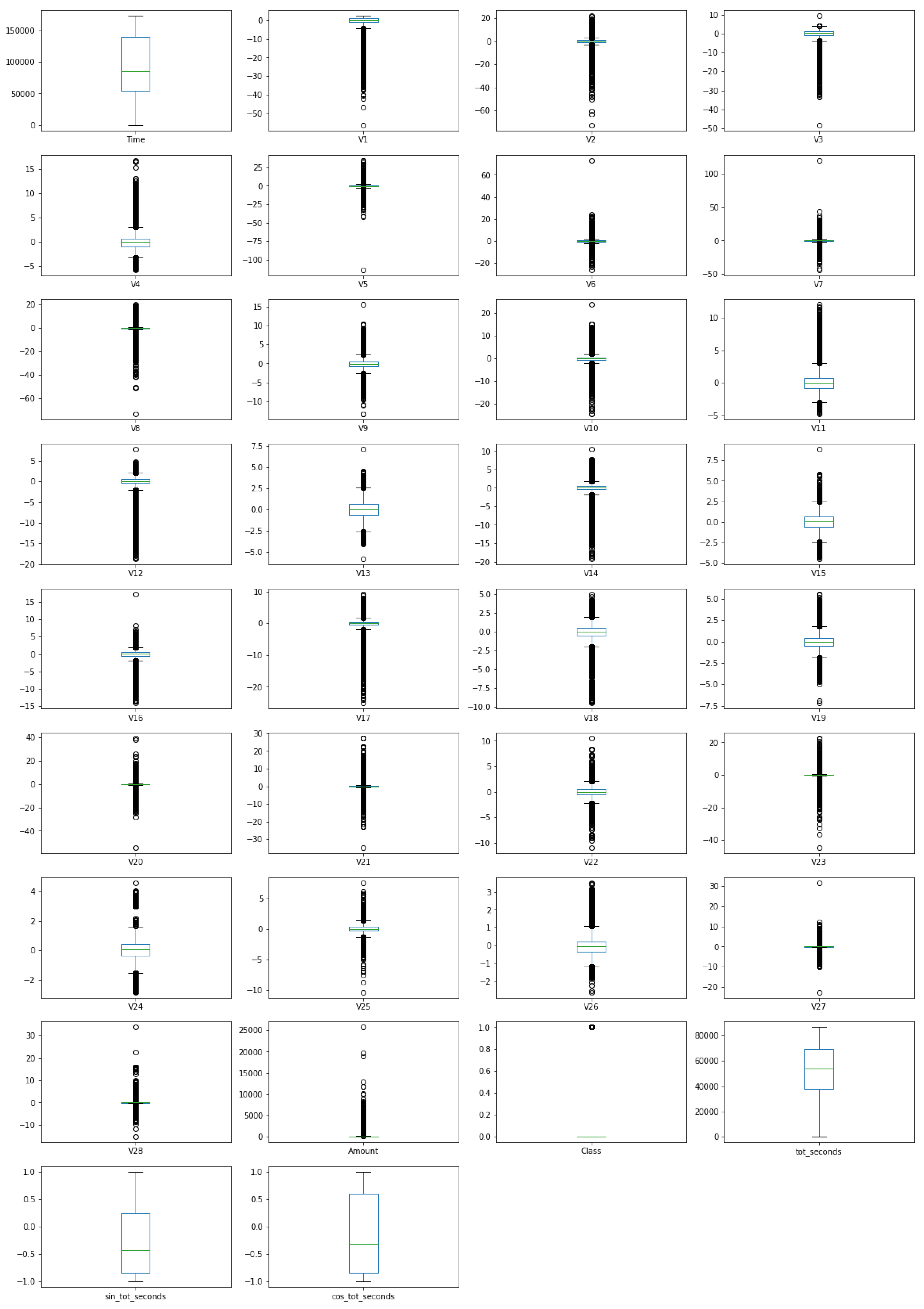
Feature Engineering and Dataset Visualisation
Feature Analysis
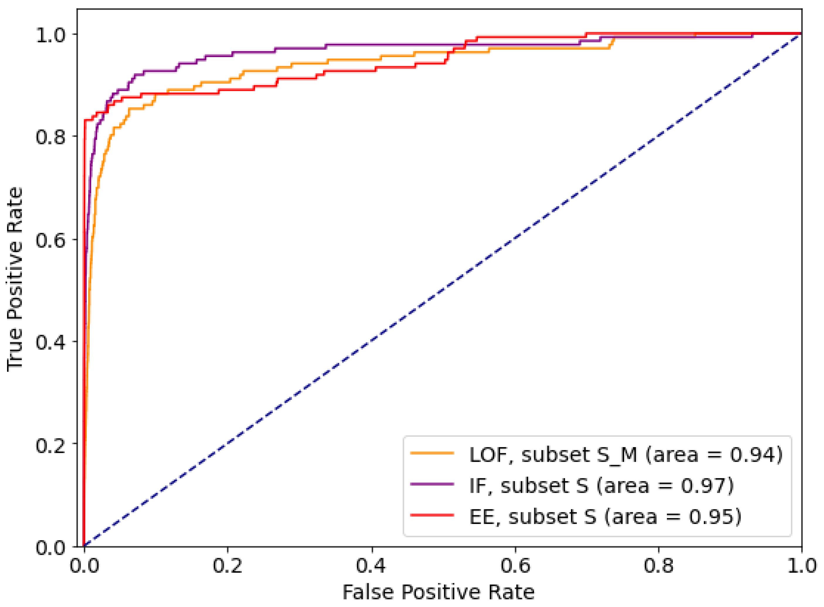
5.1.2. Outlier Detection Approach
- S—dataset excluding features with Useless, Weak and Medium predictive power
- S_M—dataset excluding features with Weak and Useless predictive power
- S_M_W—dataset excluding features with Useless predictive power
- all—dataset with all features included
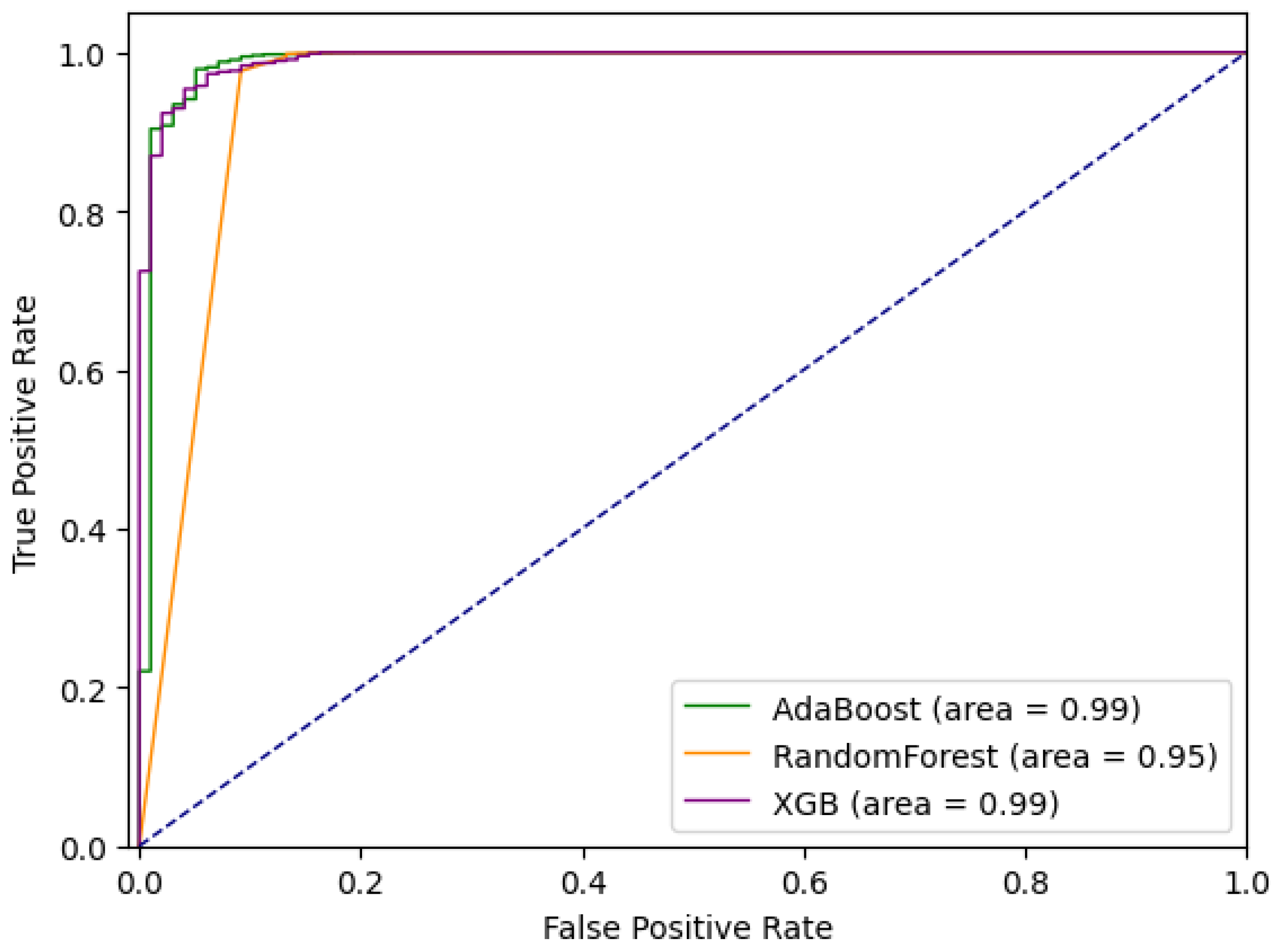
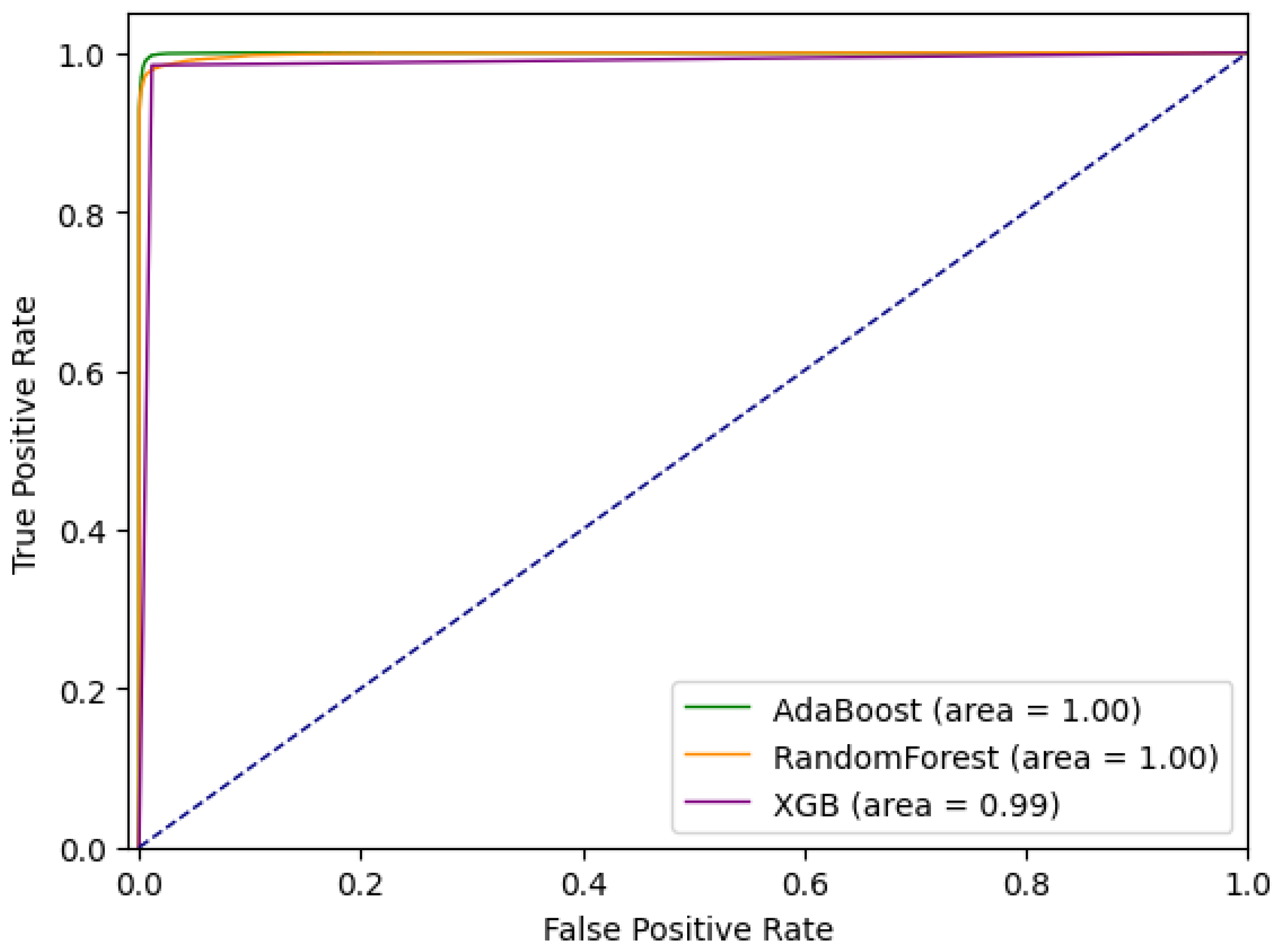
5.1.3. Ensemble Approach
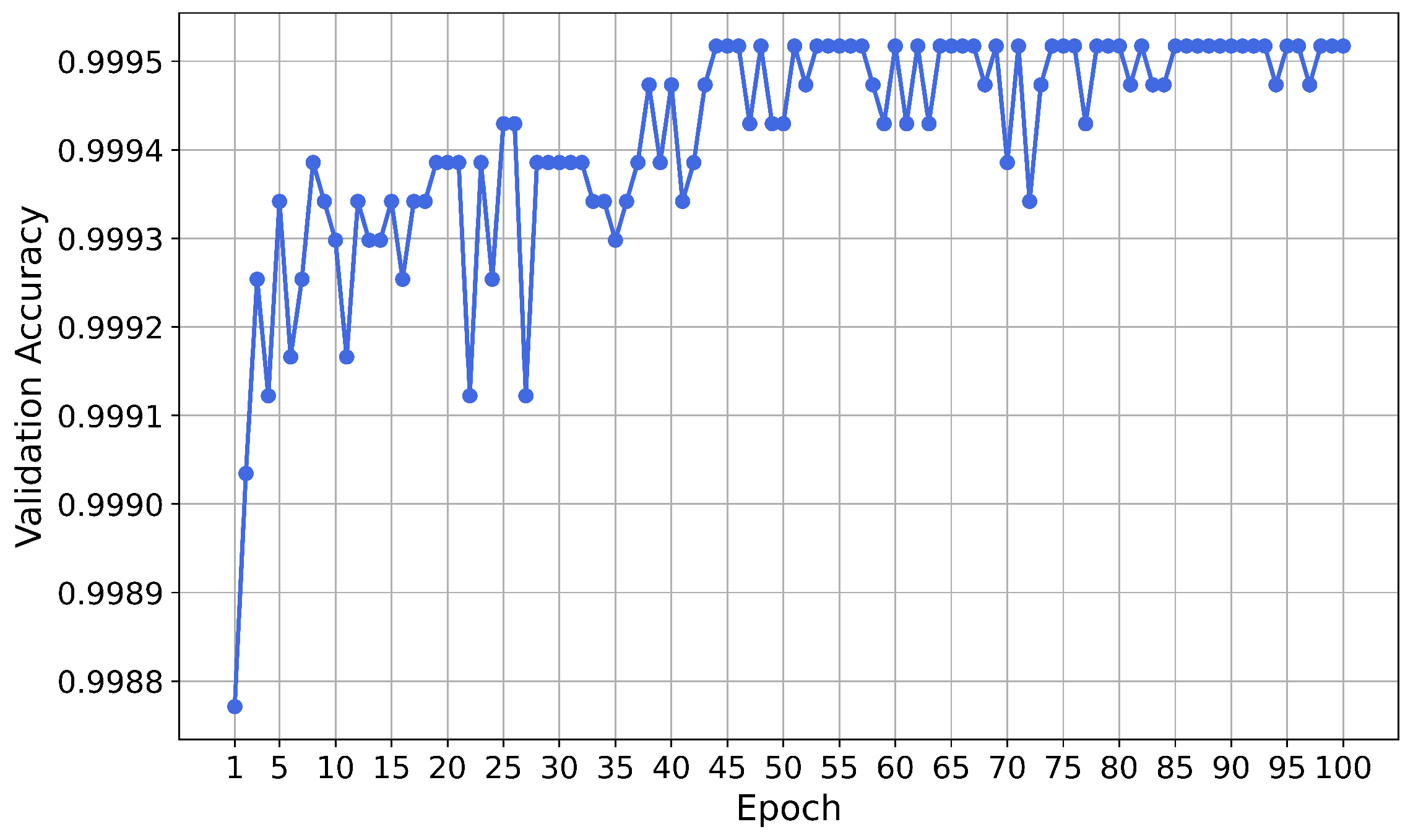
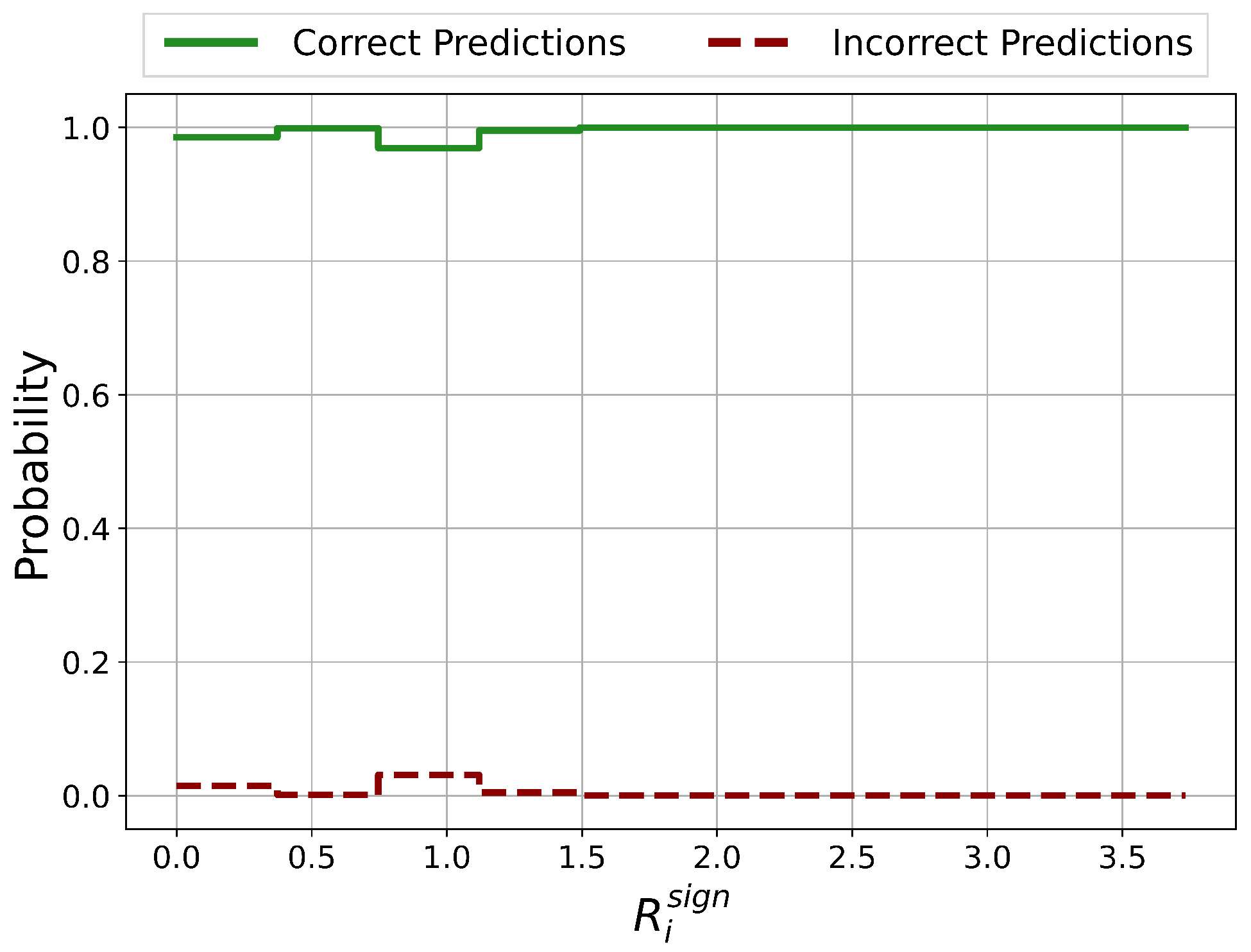
5.1.4. Reliability Analysis
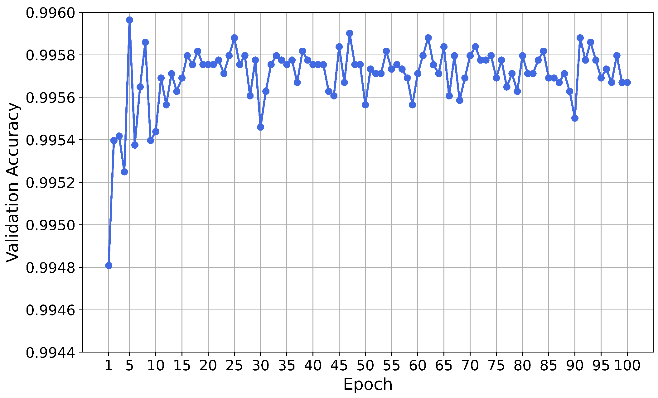
Training of the Neural Network
Results
5.2. CS#2: Financial Transactions Fraud Detection—PaySim Dataset
5.2.1. Feature Engineering and Selection
Feature Engineering and Dataset Visualisation
- hour—presenting the number of hours from the referent time point (first transaction) in 24 h time cycle, where feature range is 0–23
- day—presenting the day in the month in 30 days month cycle, where the feature range is 1–30
- weekday—presenting the day in the week in seven-day week cycle, where the feature range is 1–7
Feature Analysis
5.2.2. Outlier Detection Approach
5.2.3. Ensemble Approach
5.2.4. Reliability Analysis
Training of the Neural Network
Results
5.3. CS#3: Bank Transactions Fraud Detection—BankSim Dataset
5.3.1. Feature Engineering and Selection
Feature Engineering and Dataset Visualisation
- month—presenting the month where the feature range is 1–6
- day—presenting the day in the month in 30 days month cycle, where the feature range is 1–30
- weekday—presenting the day in the week in seven-day week cycle, where the feature range is 1–7
Feature Analysis
5.3.2. Outlier Detection Approach
5.3.3. Ensemble Approach
5.3.4. Reliability Analysis
Training of the Neural Network
Results
Reliability Analysis Results Discussion
6. Discussion on Implications of Fraud to Society and Call for Action
7. Conclusions and Future Work
Author Contributions
Funding
Institutional Review Board Statement
Informed Consent Statement
Data Availability Statement
Acknowledgments
Conflicts of Interest
References
- Bettinger, A. FINTECH: A Series of 40 Time Shared Models Used at Manufacturers Hanover Trust Company. Interfacec 1972, 2, 62–63. [Google Scholar]
- Thakor, A.V. Fintech and banking: What do we know? J. Financ. Intermed. 2020, 41. [Google Scholar] [CrossRef]
- Arner, D.W.; Barberis, J.; Buckley, R.P. The Evolution of Fintech: A New Post-Crisis Paradigm? Available online: https://heinonline.org/HOL/LandingPage?handle=hein.journals/geojintl47&div=41&id=&page= (accessed on 23 February 2021).
- PwC’s Global Economic Crime and Fraud Survey 2020. Available online: https://www.pwc.com/fraudsurvey (accessed on 30 November 2020).
- 2020 ACFE Report to the Nations. Available online: https://www.acfe.com/report-to-the-nations/2020/ (accessed on 11 November 2020).
- Fraud Definition—Investopedia. Available online: https://www.investopedia.com/terms/f/fraud.asp (accessed on 15 December 2020).
- Chalapathy, R.; Chawla, S. Deep Learning for Anomaly Detection: A Survey. arXiv 2019, arXiv:1901.03407. [Google Scholar]
- Zimek, A.; Schubert, E. Outlier Detection. In Encyclopedia of Database Systems; Liu, L., Özsu, M.T., Eds.; Springer New York: New York, NY, USA, 2017; pp. 1–5. [Google Scholar] [CrossRef]
- Credit Card Fraud Detection. Available online: https://www.kaggle.com/mlg-ulb/creditcardfraud (accessed on 30 November 2020).
- Bank Transaction Data. Available online: https://www.kaggle.com/apoorvwatsky/bank-transaction-data (accessed on 30 November 2020).
- Bitcoin Blockchain Historical Data. Available online: https://www.kaggle.com/bigquery/bitcoin-blockchain (accessed on 30 November 2020).
- UC Irvine ML Repository. Available online: https://archive.ics.uci.edu/ml/index.php (accessed on 11 November 2020).
- Synthetic Data from a Financial Payment System. Available online: https://www.kaggle.com/ntnu-testimon/banksim1 (accessed on 30 November 2020).
- Lopez-Rojas, E.A.; Elmir, A.; Axelsson, S. Paysim: A financial mobile money simulator for fraud detection. In Proceedings of the 28th European Modeling and Simulation Symposium (EMSS’16), Larnaca, Cyprus, 26–28 September 2016. [Google Scholar]
- Dal Pozzolo, A.; Boracchi, G.; Caelen, O.; Alippi, C.; Bontempi, G. Credit card fraud detection and concept-drift adaptation with delayed supervised information. In Proceedings of the 2015 International Joint Conference on Neural networks (IJCNN), Killarney, Ireland, 12–17 July 2015; pp. 1–8. [Google Scholar]
- Dal Pozzolo, A.; Boracchi, G.; Caelen, O.; Alippi, C.; Bontempi, G. Credit card fraud detection: A realistic modeling and a novel learning strategy. IEEE Trans. Neural Netw. Learn. Syst. 2017, 29, 3784–3797. [Google Scholar] [PubMed]
- Ma, T.; Qian, S.; Cao, J.; Xue, G.; Yu, J.; Zhu, Y.; Li, M. An Unsupervised Incremental Virtual Learning Method for Financial Fraud Detection. In Proceedings of the 2019 IEEE/ACS 16th International Conference on Computer Systems and Applications (AICCSA), Abu Dhabi, United Arab Emirates, 3–7 November 2019; pp. 1–6. [Google Scholar] [CrossRef]
- Somasundaram, A.; Reddy, S. Parallel and incremental credit card fraud detection model to handle concept drift and data imbalance. Neural Comput. Appl. 2019, 31, 3–14. [Google Scholar] [CrossRef]
- Ngai, E.W.T.; Hu, Y.; Wong, Y.H.; Chen, Y.; Sun, X. The application of data mining techniques in financial fraud detection: A classification framework and an academic review of literature. Decis. Support Syst. 2011, 50, 559–569. [Google Scholar] [CrossRef]
- Ahmed, M.; Mahmood, A.N.; Islam, M.R. A survey of anomaly detection techniques in financial domain. Future Gener. Comput. Syst. 2016, 55, 278–288. [Google Scholar] [CrossRef]
- Ahmed, M.; Choudhury, N.; Uddin, S. Anomaly detection on big data in financial markets. In Proceedings of the 2017 IEEE/ACM International Conference on Advances in Social Networks Analysis and Mining (ASONAM), Sydney, Australia, 31 July–3 August 2017; pp. 998–1001. [Google Scholar]
- Abdallah, A.; Aizaini, M.; Zainal, M.A. Fraud detection system: A survey. J. Netw. Comput. Appl. 2016, 68, 90–113. [Google Scholar] [CrossRef]
- Gai, K.; Qiu, M.; Sun, X. A survey on FinTech. J. Netw. Comput. Appl. 2018, 103, 262–273. [Google Scholar] [CrossRef]
- Ryman-Tubb, N.F.; Krause, P.J.; Garn, W. How Artificial Intelligence and machine learning research impacts payment card fraud detection: A survey and industry benchmark. Eng. Appl. Artif. Intell. 2018, 76, 130–157. [Google Scholar] [CrossRef]
- West, J.; Bhattacharya, M. Intelligent financial fraud detection: A comprehensive review. Comput. Secur. 2016, 57, 47–66. [Google Scholar] [CrossRef]
- Pourhabibi, T.; Ongb, K.L.; Kama, B.H.; Boo, Y.L. Fraud detection: A systematic literature review of graph-based anomaly detection approaches. Decis. Support Syst. 2020, 133, 113303. [Google Scholar] [CrossRef]
- Bao, W.; Yue, J.; Rao, Y. A deep learning framework for financial time series using stacked autoencoders and long-short term memory. PLoS ONE 2017, 12, e0180944. [Google Scholar] [CrossRef] [PubMed] [Green Version]
- Singh, A. Anomaly detection for temporal data using long short-term memory (lstm). IFAC-PapersOnLine 2017, 52, 2408–2412. [Google Scholar]
- Sorournejad, S.; Zojaji, Z.; Ebrahimi Atani, R.; Monadjemi, A.H. A Survey of Credit Card Fraud Detection Techniques: Data and Technique Oriented Perspective. arXiv 2016, arXiv:1611.06439. [Google Scholar]
- Puh, M.; Brkić, L. Detecting Credit Card Fraud Using Selected Machine Learning Algorithms. In Proceedings of the 42nd International Convention on Information and Communication Technology, Electronics and Microelectronics (MIPRO), Opatija, Croatia, 20–24 May 2019. [Google Scholar]
- Awoyemi, J.O.; Adetunmbi, A.O.; Oluwadare, S.A. Credit card fraud detection using machine learning techniques: A comparative analysis. In Proceedings of the 2017 International Conference on Computing Networking and Informatics (ICCNI), Lagos, Nigeria, 29–31 October 2017. [Google Scholar]
- Singh, A.; Jain, A. An Empirical Study of AML Approach for Credit Card Fraud Detection–Financial Transactions. Int. J. Comput. Commun. Control 2019, 14, 670–690. [Google Scholar] [CrossRef] [Green Version]
- Lucas, Y.; Jurgovsky, J. Credit card fraud detection using machine learning: A survey. arXiv 2020, arXiv:2010.06479. [Google Scholar]
- Yazici, Y. Approaches to Fraud Detection on Credit Card Transactions Using Artificial Intelligence Methods. arXiv 2020, arXiv:2007.14622. [Google Scholar]
- Bahnsen, A.C.; Stojanović, A.; Aouada, D.; Ottersten, B. Improving Credit Card Fraud Detection with Calibrated Probabilities. In Proceedings of the 2014 SIAM International Conference on Data Mining, Philadelphia, PA, USA, 24–26 April 2014. [Google Scholar]
- Dal Pozzolo, A.; Caelen, O.; Johnson, R.A.; Bontempi, G. Calibrating probability with undersampling for unbalanced classification. In Proceedings of the 2015 IEEE Symposium Series on Computational Intelligence, Cape Town, South Africa, 8–10 December 2015; pp. 159–166. [Google Scholar]
- Carcillo, F.; Dal Pozzolo, A.; Le Borgne, Y.A.; Caelen, O.; Mazzer, Y.; Bontempi, G. Scarff: A scalable framework for streaming credit card fraud detection with spark. Inf. Fusion 2018, 41, 182–194. [Google Scholar] [CrossRef] [Green Version]
- Carcillo, F.; Le Borgne, Y.A.; Caelen, O.; Bontempi, G. Streaming active learning strategies for real-life credit card fraud detection: Assessment and visualization. Int. J. Data Sci. Anal. 2018, 5, 285–300. [Google Scholar] [CrossRef] [Green Version]
- Lebichot, B.; Le Borgne, Y.A.; He-Guelton, L.; Oblé, F.; Bontempi, G. Deep-learning domain adaptation techniques for credit cards fraud detection. In Proceedings of the INNS Big Data and Deep Learning Conference; Springer: Cham, Switzerland, 2019; pp. 78–88. [Google Scholar]
- Roy, A.; Sun, J.; Mahoney, R.; Alonzi, L.; Adams, S.; Beling, P. Deep Learning Detecting Fraud in Credit Card Transactions. In Proceedings of the 2018 Systems and Information Engineering Design Symposium (SIEDS), Charlottesville, VA, USA, 27 April 2018. [Google Scholar]
- Pumsirirat, A.; Yan, L. Credit Card Fraud Detection Using Deep Learning based on Auto-Encoder and Restricted Boltzmann Machine. Available online: https://thesai.org/Downloads/Volume9No1/Paper_3-Credit_Card_Fraud_Detection_Using_Deep_Learning.pdf (accessed on 23 February 2021).
- Welcome to H2O3. Available online: http://docs.h2o.ai/h2o/latest-stable/h2o-docs/welcome.html (accessed on 11 December 2020).
- Keras: The Python Deep Learning API. Available online: https://keras.io/ (accessed on 30 November 2020).
- Bhattacharyyaa, S.; Jha, S.; Tharakunnel, K.; Westland, C. Data mining for credit card fraud: A comparative study. Decis. Support Syst. 2011, 50, 602–613. [Google Scholar] [CrossRef]
- Behera, T.K.; Panigrahi, S. Credit Card Fraud Detection: A Hybrid Approach Using Fuzzy Clustering & Neural Network. In Proceedings of the 2015 Second International Conference on Advances in Computing and Communication Engineering (ICACCE’15), Dehradun, India, 1–2 May 2015; pp. 494–499. [Google Scholar]
- Sahin, Y.; Duman, E. Detecting credit card fraud by ANN and logistic regression. In Proceedings of the 2011 International Symposium on Innovations in Intelligent Systems and Applications (INISTA), Istanbul, Turkey, 15–18 June 2011; pp. 315–319. [Google Scholar]
- Carminati, M.; Caron, R.; Maggi, F.; Epifani, I.; Zanero, S. BankSealer: A decision support system for online banking fraud analysis and investigation. Comput. Secur. 2015, 53. [Google Scholar] [CrossRef] [Green Version]
- Bahnsen, A.C.; Aouada, D.; Ottersten, B. Ensemble of Example-Dependent Cost-Sensitive Decision Trees. arXiv 2015, arXiv:1505.04637. [Google Scholar]
- Dai, Y.; Yan, J.; Tang, X.; Zhao, H.; Guo, M. Online Credit Card Fraud Detection: A Hybrid Framework with Big Data Technologies. In Proceedings of the IEEE International Conference on Trust, Security and Privacy in Computing and Communications (TrustCom), Tianjin, China, 23–26 August 2016. [Google Scholar]
- Xuan, S.; Liu, G.; Li, Z.; Zheng, L.; Wang, S.; Jiang, C. Random Forest for Credit Card Fraud Detection. In Proceedings of the 2018 IEEE 15th International Conference on Networking, Sensing and Control (ICNSC), Zhuhai, China, 27–29 March 2018. [Google Scholar]
- Zhang, X.; Han, Y.; Xu, W.; Wang, Q. HOBA: A novel feature engineering methodology for credit card fraud detection with a deep learning architecture. Inf. Sci. 2019. [Google Scholar] [CrossRef]
- Lucas, Y.; Portier, P.E.; Laporte, L.; He-Guelton, L.; Caelen, O.; Granitzer, M.; Calabretto, S. Towards automated feature engineering for credit card fraud detection using multi-perspective HMMs. Future Gener. Comput. Syst. 2020, 102, 393–402. [Google Scholar] [CrossRef]
- Chang, J.S.; Chang, W.H. A cost-effective method for early fraud detection in online auctions. In Proceedings of the 2012 Tenth International Conference on ICT and Knowledge Engineering, Bangkok, Thailand, 21–23 November 2012. [Google Scholar]
- Webga, K.; Lu, A. Discovery of rating fraud with real-time streaming visual analytics. In Proceedings of the IEEE Symposium on Visualization for Cyber Security (VizSec), Chicago, IL, USA, 25 October 2015. [Google Scholar]
- Le Khac, N.A.; Kechadi, M.T. Application of Data Mining for Anti-money Laundering Detection: A Case Study. In Proceedings of the 2010 IEEE International Conference on Data Mining Workshops, Sydney, Australia, 13 December 2010; pp. 577–584. [Google Scholar]
- Magomedov, S.; Pavelyev, S.; Ivanova, I.; Dobrotvorsky, A.; Khrestina, M.; Yusubaliev, T. Anomaly Detection with Machine Learning and Graph Databases in Fraud Management. Available online: https://thesai.org/Downloads/Volume9No11/Paper_4-Anomaly_Detection_with_Machine_Learning.pdf (accessed on 23 February 2021).
- Huang, D.; Mu, D.; Yang, L.; Cai, X. CoDetect: Financial Fraud Detection with Anomaly Feature Detection. IEEE Access 2018, 6, 19161–19174. [Google Scholar] [CrossRef]
- Amarasinghe, T.; Aponso, A.; Krishnarajah, N. Critical Analysis of Machine Learning Based Approaches for Fraud Detection in Financial Transactions. In Proceedings of the 2018 International Conference on Machine Learning Technologies (ICMLT’18), Nanchang, China, 21–23 June 2018; pp. 12–17. [Google Scholar]
- La, H.J.; Kim, S.D. A Machine Learning Framework for Adaptive FinTech Security Provisioning. J. Internet Technol. 2018, 19, 1545–1553. [Google Scholar]
- Chang, W.H.; Chang, J.S. Using clustering techniques to analyze fraudulent behavior changes in online auctions. In Proceedings of the 2010 International Conference on Networking and Information Technology, Manila, Philippines, 11–12 June 2010; pp. 34–38. [Google Scholar]
- Glancy, F.H.; Yadav, S.B. A computational model for financial reporting fraud detection. Decis. Support Syst. 2011, 50, 595–601. [Google Scholar] [CrossRef]
- Torgo, L.; Lopes, E. Utility-Based Fraud Detection. In Proceedings of the Twenty-Second International Joint Conference on Artificial Intelligence (IJCAI’11), Barcelona, Spain, 16–22 July 2011. [Google Scholar]
- Yaram, S. Machine learning algorithms for document clustering and fraud detection. In Proceedings of the 2016 International Conference on Data Science and Engineering (ICDSE), Cochin, India, 23–25 August 2016; pp. 1–6. [Google Scholar]
- Xu, J.J.; Lu, Y.; Chau, M. P2P Lending Fraud Detection: A Big Data Approach. In Proceedings of the Pacific-Asia Workshop on Intelligence and Security Informatics (PAISI), Ho Chi Minh City, Vietnam, 19 May 2015. [Google Scholar]
- Leite, R.A.; Gschwandtner, T.; Miksch, S.; Gstrein, E.; Kuntner, J. Visual analytics for event detection: Focusing on fraud. Vis. Inform. 2018, 2, 198–212. [Google Scholar] [CrossRef]
- Leite, R.A.; Gschwandtner, T.; Miksch, S.; Kriglstein, S.; Pohl, M.; Gstrein, E.; Kuntner, J. EVA: Visual Analytics to Identify Fraudulent Events. IEEE Trans. Vis. Comput. Graph. 2017, 24, 330–339. [Google Scholar] [CrossRef] [PubMed]
- Wedge, R.; Kanter, J.M.; Veeramachaneni, K.; Rubio, S.M.; Perez, S.I. Solving the false positives problem in fraud prediction using automated feature engineering. In Proceedings of the Joint European Conference on Machine Learning and Knowledge Discovery in Databases, Dublin, Ireland, 10–14 September 2018; pp. 372–388. [Google Scholar]
- Long, W.; Lu, Z.; Cui, L. Deep learning-based feature engineering for stock price movement prediction. Knowl.-Based Syst. 2019, 164, 163–173. [Google Scholar] [CrossRef]
- Baesens, B.; Höppner, S.; Verdonck, T. Data engineering for fraud detection. Decis. Support Syst. 2021, 113492. [Google Scholar] [CrossRef]
- Crosby, M.; Pattanayak, P.; Verma, S.; Kalyanaraman, V. BlockChain Technology: Beyond Bitcoin. Available online: http://scet.berkeley.edu/wp-content/uploads/AIR-2016-Blockchain.pdf (accessed on 23 February 2021).
- Xu, J.J. Are blockchains immune to all malicious attacks? Financ. Innov. 2016, 2. [Google Scholar] [CrossRef] [Green Version]
- 51% Attack. Available online: https://www.investopedia.com/terms/1/51-attack.asp (accessed on 3 December 2012).
- Kroll, J.A.; Davey, I.C.; Felten, E. The Economics of Bitcoin Mining, or Bitcoin in the Presence of Adversaries. In Proceedings of the Twelfth Workshop on the Economics of Information Security (WEIS 2013), Georgetown, WA, USA, 11–12 June 2013. [Google Scholar]
- Miller, A. Feather-Forks: Enforcing a Blacklist with Sub-50% Hash Power. Available online: https://bitcointalk.org/index.php?topic=312668.0 (accessed on 23 February 2021).
- Rahouti, M.; Xiong, K.; Ghani, N. Bitcoin Concepts, Threats, and Machine-Learning Security Solutions. IEEE Access 2018, 6, 67189–67205. [Google Scholar] [CrossRef]
- Pham, T.; Lee, S. Anomaly Detection in Bitcoin Network Using Unsupervised Learning Methods; CoRR: Leawood, KS, USA, 2016. [Google Scholar]
- Ostapowicz, M.; Żbikowski, K. Detecting Fraudulent Accounts on Blockchain: A Supervised Approach. In Proceedings of the International Conference on Web Information Systems Engineering (WISE’19), Hong Kong, China, 19–22 January 2019; pp. 18–31. [Google Scholar]
- Monamo, P.; Marivate, V.; Twala, B. Unsupervised Learning for Robust Bitcoin Fraud Detection. In Proceedings of the Information Security for South Africa (ISSA), Johannesburg, South Africa, 17–18 August 2016. [Google Scholar]
- Bartoletti, M.; Pes, B.; Serusi, S. Data Mining for Detecting Bitcoin Ponzi Schemes. In Proceedings of the Crypto Valley Conference on Blockchain Technology (CVCBT), Zug, Switzerland, 20–22 June 2018. [Google Scholar]
- Chen, W.; Zheng, Z.; Ngai, E.; Zheng, P.; Zhou, Y. Exploiting Blockchain Data to Detect Smart Ponzi Schemes on Ethereum. IEEE Access 2019, 7, 37575–37586. [Google Scholar] [CrossRef]
- Podgorelec, B.; Turkanović, M.; Karakatič, S. A Machine Learning-Based Method for Automated Blockchain Transaction Signing Including Personalized Anomaly Detection. Sensors 2020, 20, 147. [Google Scholar] [CrossRef] [PubMed] [Green Version]
- Meng, W.; Tischhauser, E.W.; Wang, Q.; Wang, Y.; Han, J. When Intrusion Detection Meets Blockchain Technology: A Review. IEEE Access 2018, 6, 10179–10188. [Google Scholar] [CrossRef]
- Breunig, M.M.; Kriegel, H.P.; Ng, R.T.; Sander, J. LOF: Identifying density-based local outliers. In Proceedings of the 2000 ACM SIGMOD International Conference on Management of Data, Dallas, TX, USA, 16–18 May 2000; pp. 93–104. [Google Scholar]
- Ankerst, M.; Breunig, M.M.; Kriegel, H.P.; Sander, J. OPTICS: Ordering points to identify the clustering structure. ACM Sigmod Rec. 1999, 28, 49–60. [Google Scholar] [CrossRef]
- Ester, M.; Kriegel, H.P.; Sander, J.; Xu, X. A density-based algorithm for discovering clusters in large spatial databases with noise. KDD 1996, 96, 226–231. [Google Scholar]
- Liu, F.T.; Ting, K.M.; Zhou, Z.H. Isolation forest. In Proceedings of the 2008 Eighth IEEE International Conference on Data Mining, Pisa, Italy, 2008, 15–19 December; pp. 413–422.
- Rousseeuw, P.J.; Driessen, K.V. A Fast Algorithm for the Minimum Covariance Determinant Estimator. Technometrics 1999, 41, 212–223. [Google Scholar] [CrossRef]
- Johannemann, J.; Hadad, V.; Athey, S.; Wager, S. Sufficient representations for categorical variables. arXiv 2019, arXiv:1908.09874. [Google Scholar]
- Hancock, J.T.; Khoshgoftaar, T.M. Survey on categorical data for neural networks. J. Big Data 2020, 7, 1–41. [Google Scholar] [CrossRef] [Green Version]
- Potdar, K.; Pardawala, T.S.; Pai, C.D. A comparative study of categorical variable encoding techniques for neural network classifiers. Int. J. Comput. Appl. 2017, 175, 7–9. [Google Scholar] [CrossRef]
- McGinnis, W.D.; Siu, C.; Andre, S.; Huang, H. Category encoders: A scikit-learn-contrib package of transformers for encoding categorical data. J. Open Source Softw. 2018, 3, 501. [Google Scholar] [CrossRef] [Green Version]
- Siddiqi, N. Credit Risk Scorecards: Developing and Implementing Intelligent Credit Scoring; John Wiley & Sons: Hoboken, NJ, USA, 2012; Volume 3. [Google Scholar]
- Brotherton, D.; Lund, B. Information Value Statistic. In Proceedings of the MWSUG 2013 Conference Proceedings, Columbus, OH, USA, 22–24 September 2013. [Google Scholar]
- Ribeiro, M.T.; Singh, S.; Guestrin, C. “Why Should I Trust You?”: Explaining the Predictions of Any Classifier. arXiv 2016, arXiv:1602.049382016. [Google Scholar]
- Lundberg, S.M.; Lee, S.I. A Unified Approach to Interpreting Model Predictions. In Proceedings of the 31st International Conference on Neural Information Processing Systems; Curran Associates Inc.: Red Hook, NY, USA, 2017; pp. 4768–4777. [Google Scholar]
- Tian, Y.; Liu, G. MANE: Model-Agnostic Non-linear Explanations for Deep Learning Model. In Proceedings of the 2020 IEEE World Congress on Services (SERVICES), Beijing, China, 18–23 October 2020; pp. 33–36. [Google Scholar] [CrossRef]
- Bach, S.; Binder, A.; Montavon, G.; Klauschen, F.; Müller, K.R.; Samek, W. On Pixel-Wise Explanations for Non-Linear Classifier Decisions by Layer-Wise Relevance Propagation. PLoS ONE 2015, 10, e0130140. [Google Scholar] [CrossRef] [PubMed] [Green Version]
- Lapuschkin, S.; Wäldchen, S.; Binder, A.; Montavon, G.; Samek, W.; Müller, K.R. Unmasking Clever Hans predictors and assessing what machines really learn. Nat. Commun. 2019, 10, 1096. [Google Scholar] [CrossRef] [PubMed] [Green Version]
- Lapuschkin, S. Opening the Machine Learning Black Box With Layer-Wise Relevance Propagation. Ph.D. Thesis, Technische Universität Berlin, Berlin, Germany, 2019. [Google Scholar] [CrossRef]
- Alber, M.; Lapuschkin, S.; Seegerer, P.; Hägele, M.; Schütt, K.T.; Montavon, G.; Samek, W.; Müller, K.R.; Dähne, S.; Kindermans, P.J. iNNvestigate Neural Networks! J. Mach. Learn. Res. 2019, 20, 1–8. [Google Scholar]
- Lapuschkin, S.; Binder, A.; Montavon, G.; Müller, K.R.; Samek, W. The LRP Toolbox for Artificial Neural Networks. J. Mach. Learn. Res. 2016, 17, 1–5. [Google Scholar]
- Glorot, X.; Bengio, Y. Understanding the difficulty of training deep feedforward neural networks. Proc. Mach. Learn. Res. 2010, 9, 249–256. [Google Scholar]
- Kingma, D.P.; Ba, J. Adam: A Method for Stochastic Optimization. arXiv 2017, arXiv:1412.6980. [Google Scholar]
- Synthetic Financial Datasets for Fraud Detection. Available online: https://www.kaggle.com/ntnu-testimon/paysim1 (accessed on 30 November 2020).
- Patne, A. Bank Statement Analysis for Detecting Fraudulent Transactions/Money Laundering 2018. Available online: https://github.com/apoorvpatne10/bank-statement-analysis (accessed on 30 November 2020).
- Money Laundering—Financial Action Task Force (FATF). Available online: https://www.fatf-gafi.org/faq/moneylaundering/ (accessed on 5 February 2021).
- Convention on International Trade in Endangered Species of Wild Fauna and Flora. Available online: https://cites.org/eng/disc/text.php (accessed on 5 February 2021).
- Pasquale, F. The Black Box Society: The Secret Algorithms That Control Money and Information; Harvard University Press: Cambridge, MA, USA, 2015. [Google Scholar]


| Technique | Map | Pro’s and Con’s |
|---|---|---|
| One Hot Encoding | Each category is mapped to a vector containing 1 and 0 to show presence or absence of feature. | Resulting in additional columns slowing down learning in the case that there are many different categories in a feature. |
| Label Encoding | Each category is getting a value from 1 to N (N is the number of categories). | An algorithm might consider an order indicated by the encoding which does not reflect the original categories. |
| Frequency Encoding | It uses the frequency of the categories as labels. | In the case that the frequency is related to the targeted variable, it is advantageous for the model. |
| Weight of Evidence Encoding | It is a measure to estimate its support (or the opposite) to a hypothesis. | The method was developed for building predictive models for a risk-evaluation of loan default in the credit and financial industry. |
| Hashing Encoding | Map variables to a higher dimensional space of integers. | This method pays off in the case of a high cardinality of categorical variables. |
| Leave One Out Encoding | It uses the mean of the target variable for all records (except current one). | Different encoding in training and validation/ test data. |
| Information Value | Variable Predictiveness |
|---|---|
| <0.02 | Not useful for prediction |
| 0.02–0.1 | Weak predictive power |
| 0.1–0.3 | Medium predictive power |
| >0.3 | Strong predictive power |
| Layer | Number of Neurons | Activation Function |
|---|---|---|
| Input layer | 23 | none |
| Dense layer 1 | 500 | ReLU |
| Dense layer 2 | 200 | ReLU |
| Output layer | 2 | softmax |
| Dataset name | Credit Card Fraud Detection |
| Domain | Credit Cards |
| Url | https://www.kaggle.com/mlg-ulb/creditcardfraud (accessed on 30 November 2020) |
| Year | 2013 |
| Type | Real data |
| Subset | creditcard.csv |
| Annotated | Yes |
| Unbalanced | Yes |
| No. of entries | 284,807 |
| Contamination rate | % |
| Time duration | 2 days |
| No. of features | 31 |
| List of features | Time, V1, V2, V3, V4, V5, V6, V7, V8, V9, V10, V11, V12, V13, V14, V15, V16, V17, V18, V19, V20, V21, V22, V23, V24, V25, V26, V27, V28, Amount, Class |
| Dataset name | Synthetic Financial Datasets for Fraud Detection |
| Domain | Financial Transactions |
| Url | https://www.kaggle.com/ntnu-testimon/paysim1 (accessed on 30 November 2020) |
| Year | 2015 |
| Type | Synthetic data |
| Subset | PS_20174392719_1491204439457_log.csv |
| Annotated | Yes |
| Unbalanced | Yes |
| No. of entries | 6,362,620 |
| Contamination rate | 0.129% |
| Time duration | 1 month |
| No. of features | 11 |
| List of features | step, type, amount, nameOrig, oldbalanceOrg, newbalanceOrig, nameDest, oldbalanceDest, newbalanceDest, isFraud, isFlaggedFraud |
| Dataset name | Synthetic data from a financial payment system |
| Domain | Financial Transactions |
| Url | https://www.kaggle.com/ntnu-testimon/banksim1 (accessed on 30 November 2020) |
| Year | 2014 |
| Type | Synthetic data |
| Subset | bs140513_032310.csv |
| Annotated | Yes |
| Unbalanced | Yes |
| No. of entries | 594,643 |
| Contamination rate | % |
| Time duration | 6 months |
| No. of features | 10 |
| List of features | step, customer, age, gender, zipcodeOri, merchant, zipMerchant, category, amount, fraud |
| Subset | bsNET140513_032310.csv |
| Annotated | Yes |
| Unbalanced | Yes |
| No. of entries | 594,643 |
| Contamination rate | % |
| Time duration | 6 months |
| No. of features | 5 |
| List of features | Source, Target, Weight, typeTrans, fraud |
| Dataset name | Bank Transaction Data |
| Domain | Financial Transactions |
| Url | https://www.kaggle.com/apoorvwatsky/bank-transaction-data (accessed on 30 November 2020) |
| Year | 2017 |
| Type | Synthetic data |
| Subset | bank.xlsx |
| Annotated | No |
| Unbalanced | n/a |
| No. of entries | 116,201 |
| Contamination rate | n/a |
| Time duration | 7 months |
| No. of features | 8 |
| List of features | Account No., Date, Transaction Details, Cheque No., Value Date, Withdrawal Amount, Deposit Amount, Balance Amount |
| Strong Predictive Power | |||
|---|---|---|---|
| feature | IV | feature | IV |
| V4 | 2.46 | V1 | 0.81 |
| V14 | 2.18 | V21 | 0.75 |
| V12 | 2.04 | V6 | 0.58 |
| V3 | 1.74 | V27 | 0.56 |
| V11 | 1.72 | V18 | 0.55 |
| V10 | 1.64 | V28 | 0.54 |
| V16 | 1.27 | V5 | 0.50 |
| V2 | 1.27 | V8 | 0.42 |
| V17 | 1.11 | V20 | 0.40 |
| V9 | 1.04 | V19 | 0.38 |
| V7 | 1.00 | Amount | 0.29 |
| Medium | Weak | Useless | |||
|---|---|---|---|---|---|
| feature | IV | feature | IV | feature | IV |
| V23 | 0.14 | V24 | 0.08 | V25 | 0.01 |
| sin_tot_seconds | 0.12 | Time | 0.05 | V22 | 0.01 |
| tot_seconds | 0.11 | V26 | 0.03 | V15 | 0.00 |
| V13 | 0.02 | ||||
| cos_tot_seconds | 0.02 | ||||
| Subset | Features |
|---|---|
| S | V4, V14, V12, V3, V11, V10, V16, V2, V17, V9, V7, V1, V21, V6, V27, V18, V28, V5, V8, V20, V19, Amount |
| S_M | V4, V14, V12, V3, V11, V10, V16, V2, V17, V9, V7, V1, V21, V6, V27, V18, V28, V5, V8, V20, V19, Amount, V23, sin_tot_seconds,tot_seconds |
| S_M_W | V4, V14, V12, V3, V11, V10, V16, V2, V17, V9, V7, V1, V21, V6, V27, V18, V28, V5, V8, V20, V19, Amount, V23, sin_tot_seconds,tot_seconds, V24, Time, V26, V13, cos_tot_seconds |
| all | V4, V14, V12, V3, V11, V10, V16, V2, V17, V9, V7, V1, V21, V6, V27, V18, V28, V5, V8, V20, V19, Amount, V23, sin_tot_seconds,tot_seconds, V24, Time, V26, V13, cos_tot_seconds, V25, V22, V15 |
| Local Outlier Factor | Isolation Forest | Elliptic Envelope | ||||
|---|---|---|---|---|---|---|
| tpr | tnr | tpr | tnr | tpr | tnr | |
| S | 0.4412 | 0.9008 | 0.9265 | 0.8992 | 0.8824 | 0.9003 |
| S_M | 0.8824 | 0.8960 | 0.9118 | 0.9001 | 0.7500 | 0.8994 |
| S_M_W | 0.7574 | 0.8810 | 0.8971 | 0.8996 | 0.8456 | 0.9002 |
| all | 0.7426 | 0.8814 | 0.9044 | 0.9001 | 0.8824 | 0.9002 |
| Random Forest | Adaptive Boosting | Extreme Gradient Boosting | ||||
|---|---|---|---|---|---|---|
| tpr | tnr | tpr | tnr | tpr | tnr | |
| all | 0.7959 | 0.9999 | 0.7959 | 0.9998 | 0.8163 | 0.9999 |
| Strong Predictive Power | |||
|---|---|---|---|
| feature | IV | feature | IV |
| nameDest | 3.21 | amount | 0.76 |
| oldbalanceOrg | 2.09 | sin_hour | 0.32 |
| newbalanceOrig | 1.01 | day | 0.30 |
| is_type_TRANSFER | 0.99 | step | 0.28 |
| type | 0.79 | ||
| Medium | Weak | Useless | |||
|---|---|---|---|---|---|
| feature | IV | feature | IV | feature | IV |
| hour | 0.22 | is_type_CASH_IN | 0.05 | newbalanceDest | 0.00 |
| oldbalanceDest | 0.18 | cos_weekday | 0.05 | is_type_DEBIT | 0.00 |
| cos_hour | 0.18 | weekday | 0.05 | isFlaggedFraud | 0.00 |
| is_type_PAYMENT | 0.14 | sin_weekday | 0.03 | ||
| is_type_CASH_OUT | 0.09 | nameOrig | 0.02 | ||
| Subset | Features |
|---|---|
| S | oldbalanceOrg, newbalanceOrig, is_type_TRANSFER, amount, sin_hour, day, step |
| S_M | oldbalanceOrg, newbalanceOrig, is_type_TRANSFER, amount, sin_hour, day, step, hour, oldbalanceDest, cos_hour, is_type_PAYMENT, is_type_CASH_OUT |
| S_M_W | oldbalanceOrg, newbalanceOrig, is_type_TRANSFER, amount, sin_hour, day, step, hour, oldbalanceDest, cos_hour, is_type_PAYMENT, is_type_CASH_OUT, is_type_CASH_IN, cos_weekday, weekday, sin_weekday |
| all | oldbalanceOrg, newbalanceOrig, is_type_TRANSFER, amount, sin_hour, day, step, hour, oldbalanceDest, cos_hour, is_type_PAYMENT, is_type_CASH_OUT, is_type_CASH_IN, cos_weekday, weekday, sin_weekday, newbalanceDest, is_type_DEBIT, isFlaggedFraud |
| Local Outlier Factor | Isolation Forest | |||
|---|---|---|---|---|
| tpr | tnr | tpr | tnr | |
| S | 0.9326 | 0.8875 | 0.8283 | 0.8103 |
| S_M | 0.9248 | 0.8923 | 0.8838 | 0.8099 |
| S_M_W | 0.9240 | 0.8923 | 0.8456 | 0.8102 |
| all | 0.9257 | 0.8933 | 0.8078 | 0.8096 |
| Random Forest | Adaptive Boosting | Extreme Gradient Boosting | ||||
|---|---|---|---|---|---|---|
| tpr | tnr | tpr | tnr | tpr | tnr | |
| all | 0.9761 | 0.9793 | 0.7171 | 0.9999 | 0.8856 | 1.000 |
| Strong | Medium | Weak | |||
|---|---|---|---|---|---|
| feature | IV | feature | IV | feature | IV |
| merchant | 4.47 | is_category_wellnessandbeauty | 0.11 | is_gender_F | 0.06 |
| customer | 2.54 | is_category_home | 0.11 | is_gender_M | 0.05 |
| amount | 2.14 | is_category_otherservices | 0.10 | is_category_hyper | 0.04 |
| is_category_transportation | 1.69 | is_category_tech | 0.03 | ||
| is_category_sportsandtoys | 1.28 | ||||
| is_category_health | 0.53 | ||||
| is_category_leisure | 0.49 | ||||
| is_category_travel | 0.47 | ||||
| is_category_hotelservices | 0.28 | ||||
| Useless Predictive Power | |||
|---|---|---|---|
| feature | IV | feature | IV |
| step | 0.01 | cos_day | 0.00 |
| month | 0.01 | sin_weekday | 0.00 |
| age | 0.01 | weekday | 0.00 |
| is_category_barsandrestaurants | 0.00 | is_category_contents | 0.00 |
| is_category_food | 0.00 | is_gender_U | 0.00 |
| is_category_fashion | 0.00 | cos_weekday | 0.00 |
| is_gender_E | 0.00 | zipMerchant | 0.00 |
| day | 0.00 | zipcodeOri | 0.00 |
| sin_day | 0.00 | ||
| Local Outlier Factor | Isolation Forest | Elliptic Envelope | ||||
|---|---|---|---|---|---|---|
| tpr | tnr | tpr | tnr | tpr | tnr | |
| S | 0.8511 | 0.8908 | 0.9546 | 0.9005 | 0.8299 | 0.8998 |
| S_M | 0.8681 | 0.8891 | 0.9787 | 0.9002 | 0.8242 | 0.8995 |
| S_M_W | 0.8006 | 0.8862 | 0.9849 | 0.9005 | 0.8166 | 0.8999 |
| all | 0.2911 | 0.8989 | 0.5803 | 0.8992 | 0.3653 | 0.8994 |
| Random Forest | Adaptive Boosting | Extreme Gradient Boosting | ||||
|---|---|---|---|---|---|---|
| tpr | tnr | tpr | tnr | tpr | tnr | |
| all | 0.9956 | 0.9673 | 0.9931 | 0.9915 | 0.9885 | 0.9843 |
Publisher’s Note: MDPI stays neutral with regard to jurisdictional claims in published maps and institutional affiliations. |
© 2021 by the authors. Licensee MDPI, Basel, Switzerland. This article is an open access article distributed under the terms and conditions of the Creative Commons Attribution (CC BY) license (http://creativecommons.org/licenses/by/4.0/).
Share and Cite
Stojanović, B.; Božić, J.; Hofer-Schmitz, K.; Nahrgang, K.; Weber, A.; Badii, A.; Sundaram, M.; Jordan, E.; Runevic, J. Follow the Trail: Machine Learning for Fraud Detection in Fintech Applications. Sensors 2021, 21, 1594. https://doi.org/10.3390/s21051594
Stojanović B, Božić J, Hofer-Schmitz K, Nahrgang K, Weber A, Badii A, Sundaram M, Jordan E, Runevic J. Follow the Trail: Machine Learning for Fraud Detection in Fintech Applications. Sensors. 2021; 21(5):1594. https://doi.org/10.3390/s21051594
Chicago/Turabian StyleStojanović, Branka, Josip Božić, Katharina Hofer-Schmitz, Kai Nahrgang, Andreas Weber, Atta Badii, Maheshkumar Sundaram, Elliot Jordan, and Joel Runevic. 2021. "Follow the Trail: Machine Learning for Fraud Detection in Fintech Applications" Sensors 21, no. 5: 1594. https://doi.org/10.3390/s21051594