
A Regional Zenith Tropospheric Delay (ZTD) Model Based on GPT3 and ANN


1
College of Geoscience and Surveying Engineering, China University of Mining and Technology-Beijing, Beijing 100083, China
2
School of Geodesy and Geomatics, Wuhan University, Wuhan 430079, China
3
School of Earth Science, The Ohio State University, Columbus, OH 43210, USA
4
State Key Laboratory of Resources and Environmental Information System, Institute of Geographic Sciences and Natural Resources Research, Beijing 100101, China
*
Author to whom correspondence should be addressed.
Remote Sens. 2021, 13(5), 838; https://doi.org/10.3390/rs13050838
Submission received: 22 January 2021
/
Revised: 16 February 2021
/
Accepted: 20 February 2021
/
Published: 24 February 2021
(This article belongs to the Special Issue Climate Modelling and Monitoring Using GNSS)
Abstract
:The delays of radio signals transmitted by global navigation satellite system (GNSS) satellites and induced by neutral atmosphere, which are usually represented by zenith tropospheric delay (ZTD), are required as critical information both for GNSS positioning and navigation and GNSS meteorology. Establishing a stable and reliable ZTD model is one of the interests in GNSS research. In this study, we proposed a regional ZTD model that makes full use of the ZTD calculated from regional GNSS data and the corresponding ZTD estimated by global pressure and temperature 3 (GPT3) model, adopting the artificial neutral network (ANN) to construct the correlation between ZTD derived from GPT3 and GNSS observations. The experiments in Hong Kong using Satellite Positioning Reference Station Network (SatRet) were conducted and three statistical values, i.e., bias, root mean square error (RMSE), and compound relative error (CRE) were adopted for our comparisons. Numerical results showed that the proposed model outperformed the parameter ZTD model (Saastamoinen model) and the empirical ZTD model (GPT3 model), with an approximately 56%/52% and 52%/37% RMSE improvement in the internal and external accuracy verification, respectively. Moreover, the proposed method effectively improved the systematic deviation of GPT3 model and achieved better ZTD estimation in both rainy and rainless conditions.
1. Introduction
The radio signal is delayed and bent during its passage through the neutral atmosphere due to the interaction with water vapor particles and dry gases [1,2]. In global navigation satellite system (GNSS) application, the tropospheric delay between receiver and satellite varies from 2 to 20 m depending on the elevation angle of the satellite, making it a significant error source that should be properly handled [3,4,5]. The zenith tropospheric delay (ZTD), which is projected from the slant tropospheric delay by using the mapping function, is a common parameter to describe the tropospheric influence on signal traveling. Studies confirm that the accuracy of the ZTD has a crucial impact on GNSS positioning in terms of convergence time and accuracy [6,7,8,9,10], and the ZTD is basis for retrieving the precipitable water vapor (PWV) in GNSS meteorology [11,12,13]. Establishing a stable and reliable zenith tropospheric delay (ZTD) model is one of the interests in GNSS research.
On the basis of the relationship between the ZTD and meteorological parameters such as temperature, pressure, and water vapor pressure, researchers established a series of parameter ZTD models such as the Hopfield model, Saastamoinen model, and Black model [14,15,16]. These models can achieve ZTD values with centimeter-level accuracy by inputting accurate measured meteorological parameters [17,18]. However, most GNSS sites are not equipped with meteorological sensors, and there are often no collocated weather stations available for those sites. It is not feasible to directly use the above models to acquire the ZTD values.
Many empirical ZTD models that feedback only by location and time of the sites were developed to achieve ZTD estimates without measured meteorological parameters. Collins and Langley (1997) proposed the UNB3 model, in which the meteorological parameters are stored in the form of a look-up table with a 15° interval from the equator to the poles [19]. The modified versions of UNB model have been developed to accomplish a more accurate estimation, such as the UNB3m model, UNBw.na model, and EGNOS model [20,21,22]. These models cannot reflect zonal variation of ZTD resulting in large model errors in some areas. Li et al. established the IGGtrop model using four years of National Centers for Environment Prediction (NCEP) data based on a three-dimensional grid. The implementation of vertical levels leads to a large data volume and requires greater storage space compared with other models, making it difficult to promote this model [3]. Krueger and Schuler obtained the seasonal and diurnal variation coefficients for ZTD estimation by fitting NCEP meteorological data and established the TropGrid and TropGrid2 model [23,24,25]. Yao et al. proposed the GZTD model using the Global Geodetic Observing System (GGOS) Atmosphere data based on spherical harmonics [26] and developed the GZTD2 model considering diurnal variations [27]. Mateus et al. Developed an hourly HGPT model based on the full spatial and temporal resolution of the new ERA5 reanalysis using the time-segmentation concept [28]. On the basis of the above models, researchers proposed some other empirical ZTD models with their own characteristics, such as the IGGtrop_SH and IGGtrop_rH models [29], the GZTDS model [30], the R_GZTD model [4], the GRNN model [17], the CPT model [31], the SHAtropE model [32], and the RGZTD model [18]. In addition, the global pressure and temperature (GPT)2w model and GPT3 model, established on monthly meteorological data of 10-year (2001–2010) ERA-Interim data with a global resolution of 1° × 1° geographical grid, can also provide precise ZTD products [33,34]. The GPT3 model is the latest version, which is the one we used in this paper.
Due to the limitations of some factors, such as the time resolution and spatial resolution of the modelling data, the accuracy of the empirical ZTD model is often lower than that of the parameter ZTD model, especially when calculating ZTD in some certain regions. Taking GPT3 model, which is currently the most accurate and most commonly used one, as an example, its global average ZTD accuracy is 3.6 cm and the accuracy of most of the sites in China reached 6 cm in a validation experiment [4,33,34,35,36,37]. Considering the development of Continuously Operating Reference Station (CORS) [38], its GNSS sites can provide ZTD products with high accuracy and high time resolution, which provides opportunity for constructing a regional ZTD model with higher accuracy [39]. In this study, we proposed a new modeling method for regional ZTD empirical model, which is based on the artificial neutral network (ANN) and GPT3 model. This method makes full use of the ZTD calculated from regional GNSS data and the corresponding ZTD estimated by GPT3 model, and adopts the ANN to construct the correlation between ZTD derived from GPT3 and GNSS observations. On the basis of this modeling method, we developed a new regional ZTD model for Hong Kong on the basis of the Satellite Positioning Reference Station Network (SatRet). Experimental results show that the new model can effectively improve the regional ZTD accuracy and that it outperforms the parameter ZTD model and the empirical model.
This article is organized as follows. The GPT3 model and ANN used to establish the new regional ZTD model are introduced in Section 2. To evaluate the accuracy of the proposed model, we conducted experiments and analysis, which are described in Section 3. Section 4 discusses the performances of the proposed model in different weather conditions. The conclusions are given in Section 5.
2. Methodology
2.1. The GPT3 Model
The global pressure and temperature 3 (GPT3) model proposed by Landskron and Bohm is the up-to-date version of GPT series [33,34,40,41]. GPT3 represents a very comprehensive troposphere model that can be used for a series of geodetic as well as meteorological and climatological purposes. It provides the mean values plus annual and semiannual amplitudes of a set of meteorological quantities that are consistent with previous versions. These meteorological parameters are derived consistently from monthly mean pressure level data of ERA-Interim fields with a global resolution of 1° × 1° geographical grid. The pressure (P) in hPa, weighted mean temperature (Tm) in K, water vapor pressure (e) in hPa, and water vapor lapse rate that are used for ZTD calculation are included, and they are estimated by the following equation [41]:
where r(t) represents the meteorological parameters to be estimated; doy denotes the day of the year; A0 represents its mean value; and and are their annual and semiannual amplitudes, respectively. After obtaining the needed meteorological quantities at the four nearest sampling points, we adopt the bilinear interpolation algorithm to interpolate the parameters of the site to be determined. Then, the ZTD values are calculated by the following formulas [15,42]:
where ZHD and ZWD represent the zenith hypostatic delay and zenith wet delay, respectively, and and H are the latitude and ellipsoidal height of the site, respectively. (16.52 K/hPa) and k3 (3.776*105 K2/hPa a) are the atmospheric refractive index constants, Rd (287.0464 JK−1kg−11) denotes the dry air ratio gas constant, and gm (9.80655 m/s2) denotes the mean gravitational acceleration [42].
2.2. Artificial Neural Network
An artificial neural network (ANN) is the piece of a computing system designed to simulate the way the human brain analyzes and processes information. In principle, it can efficiently handle input and output variables relations, without limitations in linear relationships [43,44]. Two important characteristics of ANN are that they allow the user to adapt the architecture to the task itself, and that they are fully data-driven approaches that impose no limitations on the distribution of input data. The self-learning capabilities enable ANN to produce better results as enough data become available. The ANN is composed of an input layer, one or more hidden layers and an output layer, shown in Figure 1. The most important parameter in ANN models is the number of neurons and hidden layers; the greater the number of neurons and hidden layers, the higher the learning accuracy and the weaker the generalization ability. Each neuron in one layer has directed connections to the neurons of the subsequent layer and has an activation function. The activation function is used to enforce a specific behavior to each neuron/layer. Thus, ANN can be used in many tasks, e.g., classification and regression [45,46], and is also used in the geoscience field [47,48]. In this study, we utilized the ANN as a modeling tool for regional ZTD model, and adopted the MATLAB Neural Network toolbox.
2.3. The Regional ZTD Model
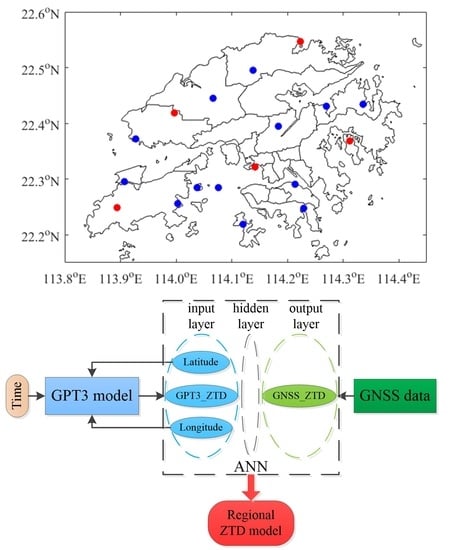
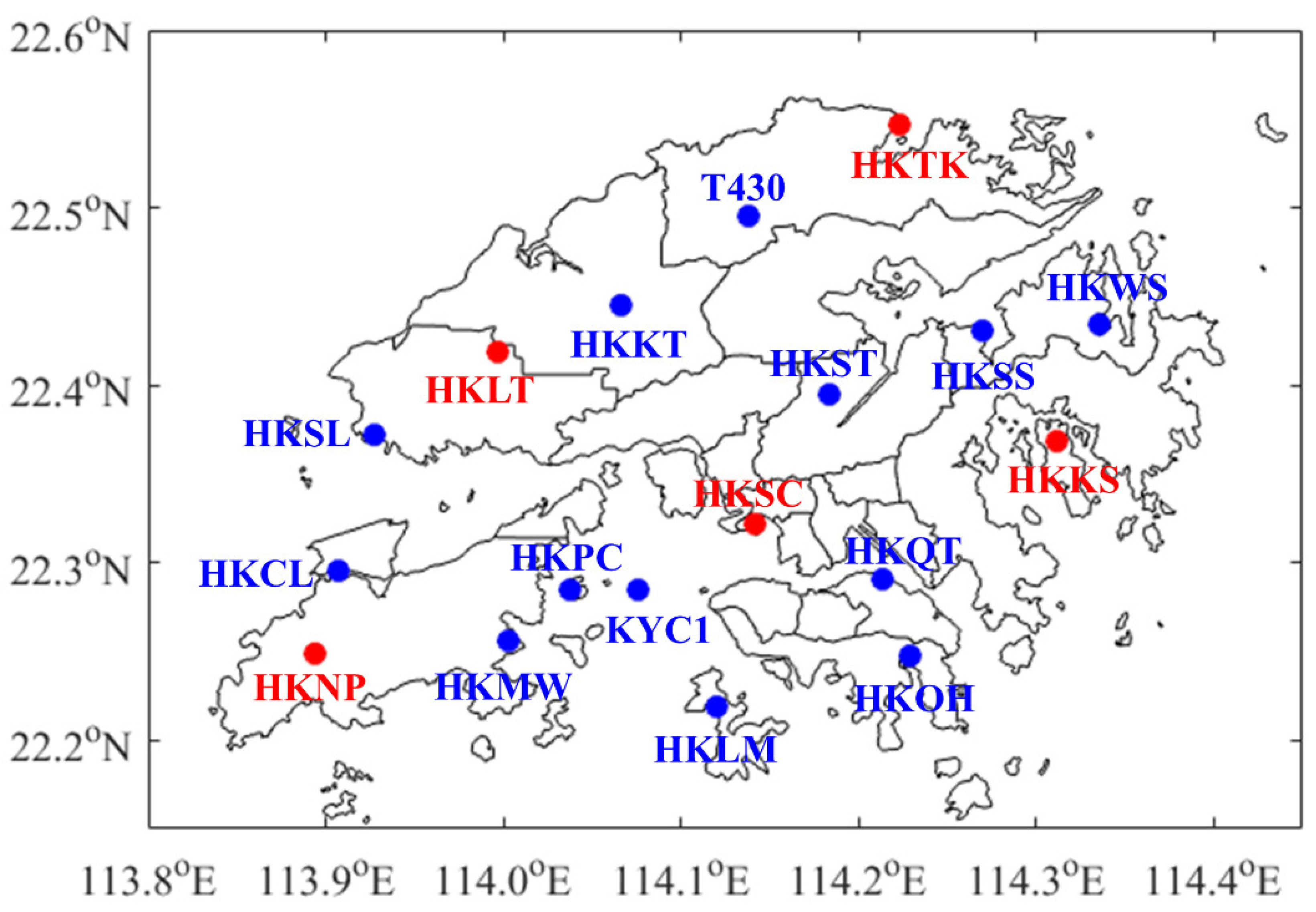
The Hong Kong Survey and Mapping Office (SMO) of the Lands Department makes use of GNSS to develop a local satellite positioning system, i.e., SatRef. It consists of 18 CORSs that are distributed in the area of 113.80°–114.45° for longitude and 22.15°–22.6° for latitude, which is shown in Figure 2. The detailed coordinates of the GNSS stations, including latitude, longitude and ellipsoid height, are listed in Table 1, and the average of the distance between the two nearest stations is 6.9km. The GNSS observation and surface meteorological data of these 18 sites can be freely downloaded via its website. On the basis of the double differenced model, we can accurately calculate the GNSS ZTD by using GAMIT 10.71 software. In this processing, the observations with a sampling rate of 30 s, a cut-off elevation of 10°, the International GNSS Service (IGS) precise ephemeris, and Global Mapping Function (GMF) are adopted [49]. To reduce the well know strong correlation of tropospheric parameters caused by the short baselines between GNSS sites [50], we incorporated 3 IGS stations (SHAO, BJFS, and LHAZ) into this solution.
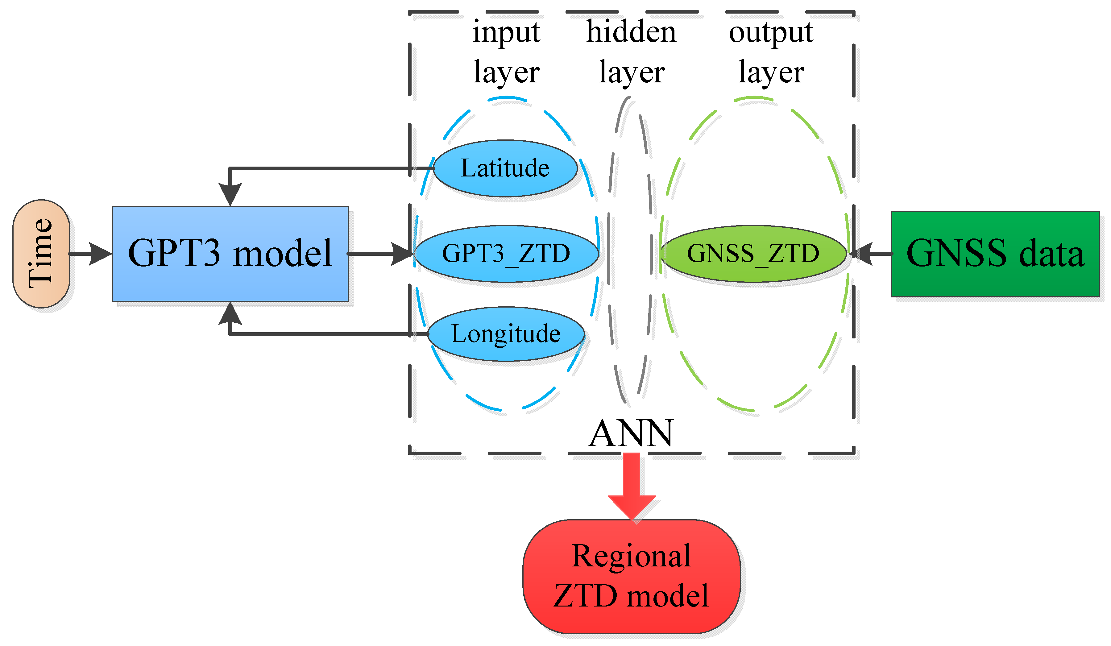
In this region, high-accuracy ZTD can be achieved at these 18 sites through GNSS data processing, which is called GNSS_ZTD. In addition, the ZTD estimates of these sites can also be easily obtained by GPT3 model without any external data, which is called GPT3_ZTD. This gives an opportunity to explore the relationship between GNSS_ZTD and GPT3_ZTD, which is the key to construct the new regional ZTD model. In this stage, we selected the latitude and longitude of the sites as well as their GPT3_ZTD as the input variables of the input layer, set the corresponding GNSS_ZTD as the output variable of the output layer, and trained them using ANN. Note that repeated trainings were tested to obtain an optimal neural network to construct the regional ZTD model, which also fed back only by location and time information. Figure 3 is a flowchart showing the basic process of constructing the regional ZTD model on the basis of GPT3 and ANN.
3. Experiment and Verification
In our experiment, the 18 GNSS sites in Figure 2 were divided into two types, which were represented by blue and red dots, respectively. Only the sites indicated by blue dots were used to construct the regional ZTD model. The GNSS observations from 13 August to 19 August, 2017 (DOY of 225 to 231, 2017) were processed to obtain GNSS_ZTD with a temporal resolution of 30 min. The corresponding GPT3_ZTD was also obtained by inputting epoch and location information to GPT3 model. The first 5 days of data from the 13 sites indicated by blue dots were used in ANN training to build the regional ZTD model, and the data from the two types (training and test) of sites on the other 2 days served as internal and external accuracy verification, respectively.
To assess the performance of the proposed ZTD model, we compared the ZTD values estimated by different models using the GNSS_ZTD as a reference. The methods for calculating ZTD in the comparison were the new regional ZTD model (Method #1), the GPT3 model (Method #2), and the Saastamoninen ZTD model (Method #3). The Saastamoninen ZTD model is the most commonly used parameter ZTD model, which can be represented by the following equation [15,51], where the parameters are the same as in Equations (2) and (3).
Three statistical quantities, i.e., bias, root mean square error (RMSE) and compound relative error (CRE), were chosen as criteria to study the comparison [52]. Different statistical values highlight different features of the results [53]. Bias is an unambiguous, natural, measure of average error, which is expressed in the same unit as the ZTD itself. RMSE is used as a measure of deviation from the observed value. It depends on the squared error means and has sensitivity to large outliers. CRE is a measure of similarity between the observed and interpolated values, namely, the ration between the mean squared error and the variance of the observed values. The equations are described as follows:
where and are the ZTD values from the different methods and the reference, respectively. N refers to the number of the samples.
3.1. Analysis of ANN Training
The datasets for ANN training contained 3120 groups of data; each group of data had latitude, longitude, and GPT3_ZTD for input layer, and GNSS_ZTD for output layer. In the training process of ANN, the datasets mentioned above were divided into a training set and validation set, accounting for 75% and 25%, respectively. The training set was used to adjust the weights on the neural network, and the validation set was used to minimize overfitting [42,44]. After repeated trainings, the ANN structure used in this paper was as follows: the input layer had three nodes, which was the same as the number of input parameters. The output layer had a single node, that is, the GNSS_ZTD. There were two hidden layers, and the number of nodes was five. The Levenberg–Marquardt and hyperbolic tangent were chosen as the training and activation functions, respectively. The maximum training number, learning rate, and error threshold were set to 6000, 0.01, and 0.001, respectively.
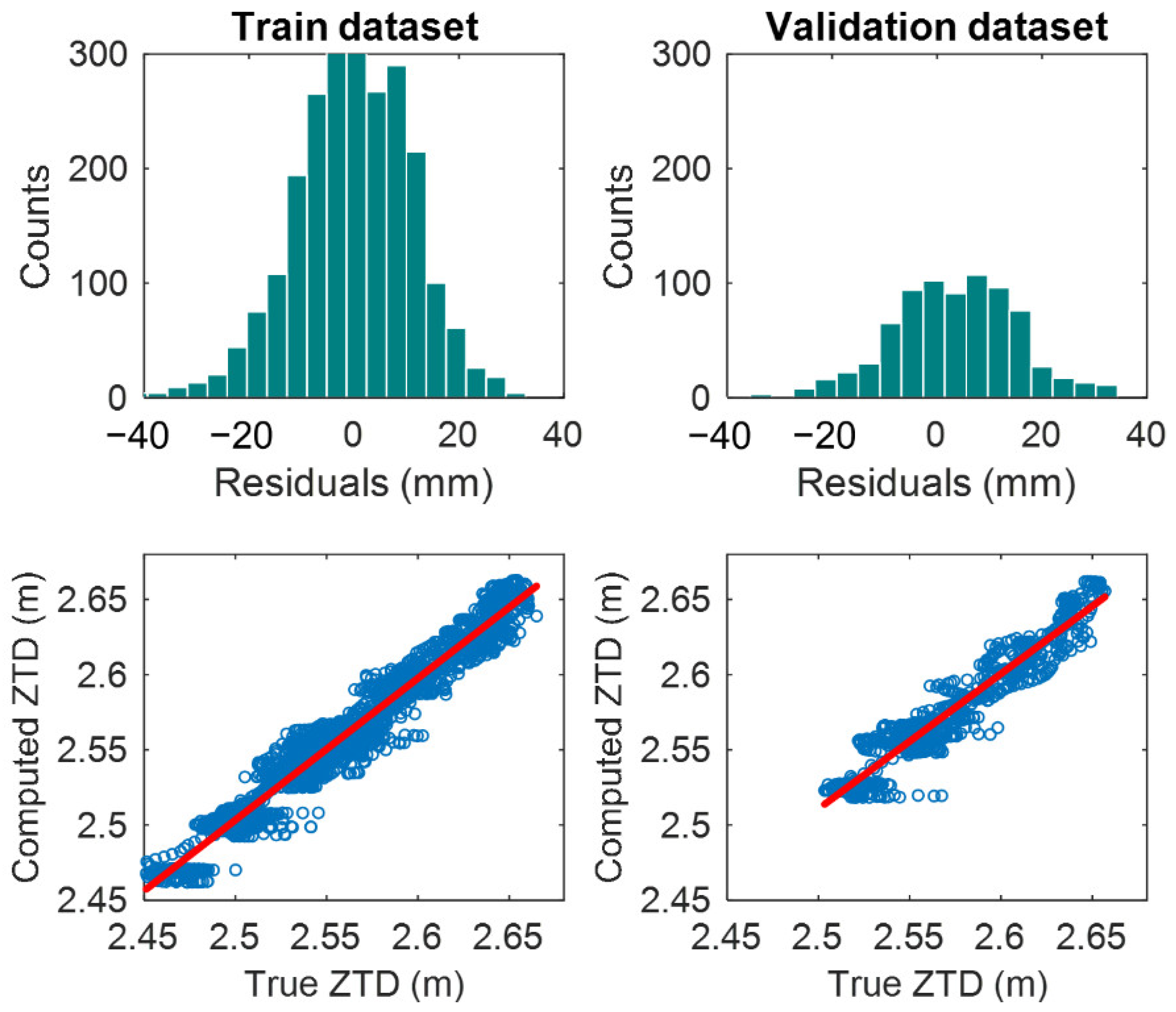
When the optimal neural network for ZTD model is achieved, the statistical indices of training set and validation set can be first used to show the accuracy assessment of the ZTD model on the basis of ANN. The RMSE and correlation coefficient were 11.08 mm/0.97 and 12.41 mm/0.95 for the training and validation set, respectively. In Figure 4, the upper panel represents the histogram of ZTD residuals for training and validation set, and the absolute value of residuals were smaller than 40 mm. For the training set, the percentage of residuals in the range of −10 to 10 mm accounted for 64%, while the percentage reached to 93% when the range was set to −20 to 20 mm. These percentages were 57% and 91% for the validation set, respectively. The lower panel of Figure 4 shows the linear regression for training and validation sets, in which the scatter points of two graphs were close to the 1:1 line. The distribution of scatter points and the straight lines showed a good linear regression relationship both in training and validation sets. Specifically, the slopes of the regression equation were 0.94 and 0.90 for the training and validation sets, respectively.
3.2. Internal Accuracy Verification
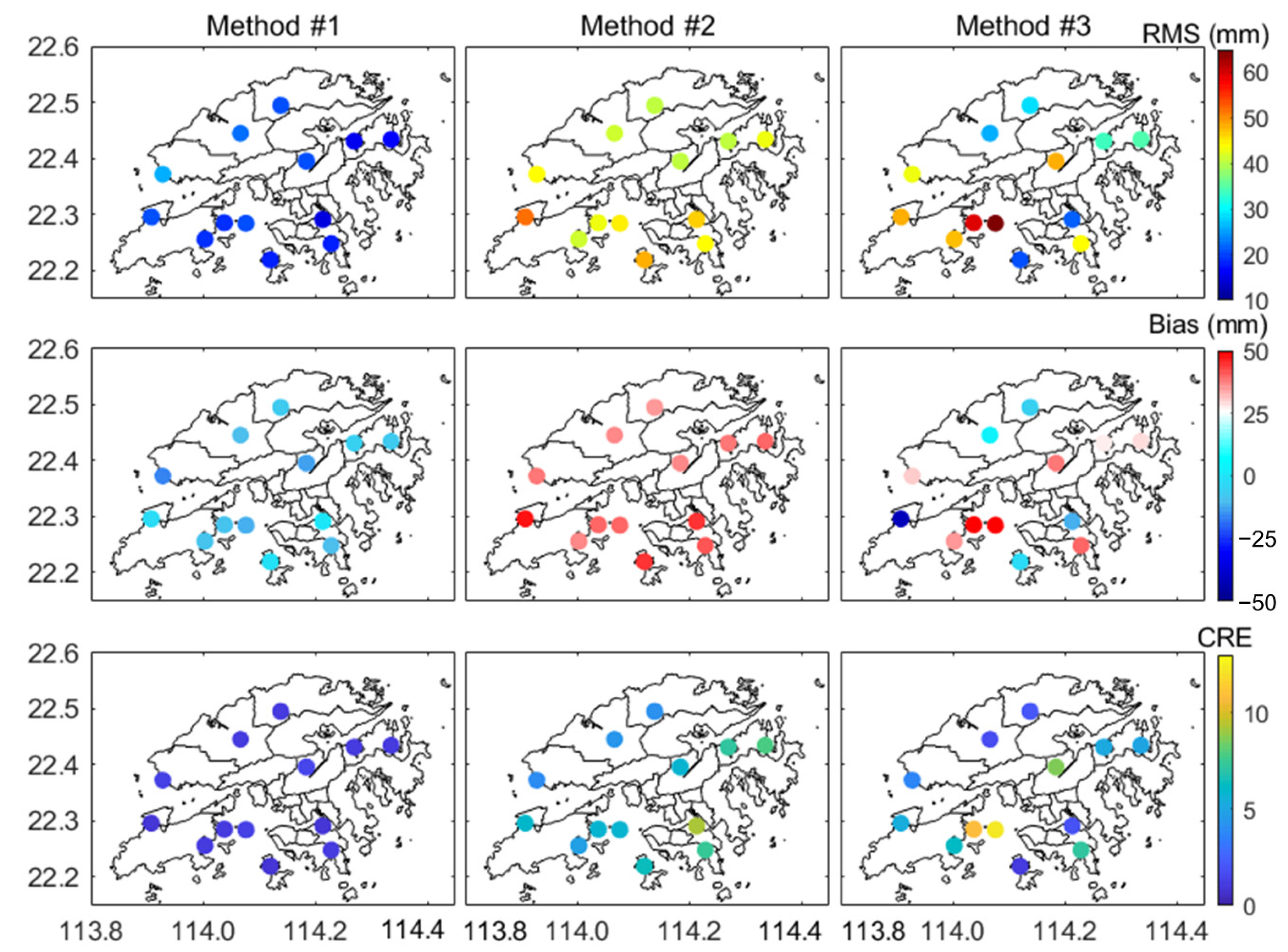
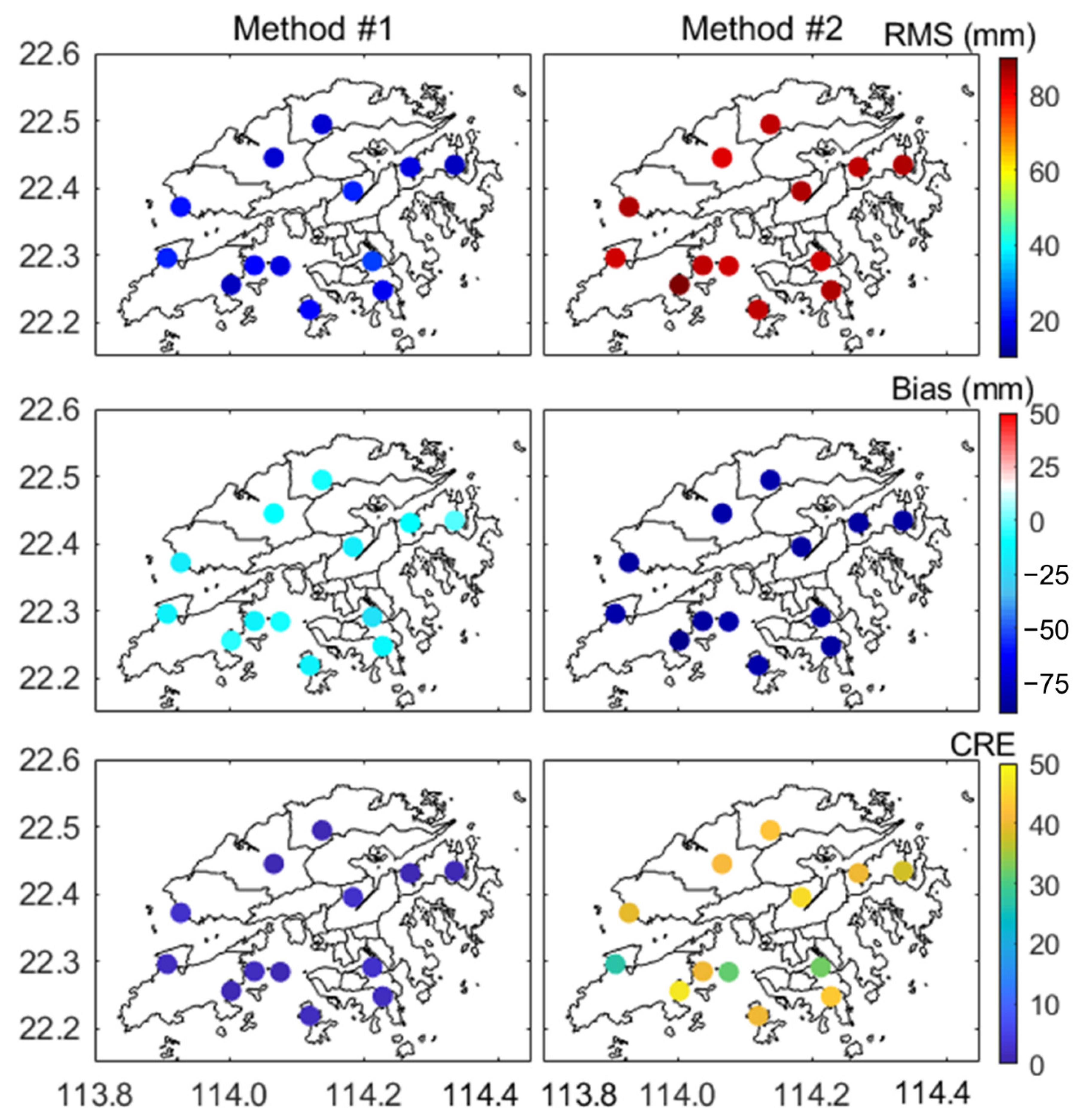
For internal accuracy verification, we adopted 13 GNSS sites used in the ZTD modelling. The statistical results, including RMSE, bias, as well as CRE, were counted for the three methods. The maps of RMSE, bias, and CRE show the different performances of the three methods at each site (Figure 5). It can be seen that the three statistical results of Method #1 at all sites were obviously better than the other methods. Compared to Method #2, Method #3 had a better performance at most of the sites, but four sites with poor performance by Method #3 can still be observed. It is particularly visible that only Method #3 had large differences in the performance of RMSE, bias, and CRE at different sites. It illustrates that the accuracy of parameter ZTD model, e.g., Saastamoinen model, is likely to be affected by the changes of location and environment of the sites, resulting in poor stability, while the empirical model such as the GPT3 model and the proposed model showed good stability in the experimental areas.
For bias, Method #1 had only one site with positive bias, and the remaining sites were negative bias; Method #2 had a positive bias large than 35 mm at all sites, and the positive and negative values of Method #3 were randomly distributed. Note that the bias of Method #1 was closer to 0 mm at each site compared to the other methods. For RMSE, Method #1 had only one site reaching 26 mm, and the remaining sites were less than 20 mm; the values of Method #2 were greater than 40 mm at all sites, and Method #3 had a large distribution, ranging from 21 to 65 mm. For CRE, their performances were similar to those of RMSE.
The mean bias, RMSE, and CRE of the differences between the ZTD derived from the three models and the referenced ZTD at all sites are summarized in Table 2. The values within square brackets are the minimum and maximum. In terms of the mean values, Method #3 performed better than Method #2, but the worst values of each statistics appeared in Method #3. One can find from the statistical results that Method #1 significantly outperformed the other two methods in terms of the minimum and maximum, as well as the mean value. Specifically, the mean RMSE and CRE of Method #1 were 19.4 mm and 1.1, respectively, having an approximately 56%/52% and 77%/80% improvement over the other two methods.
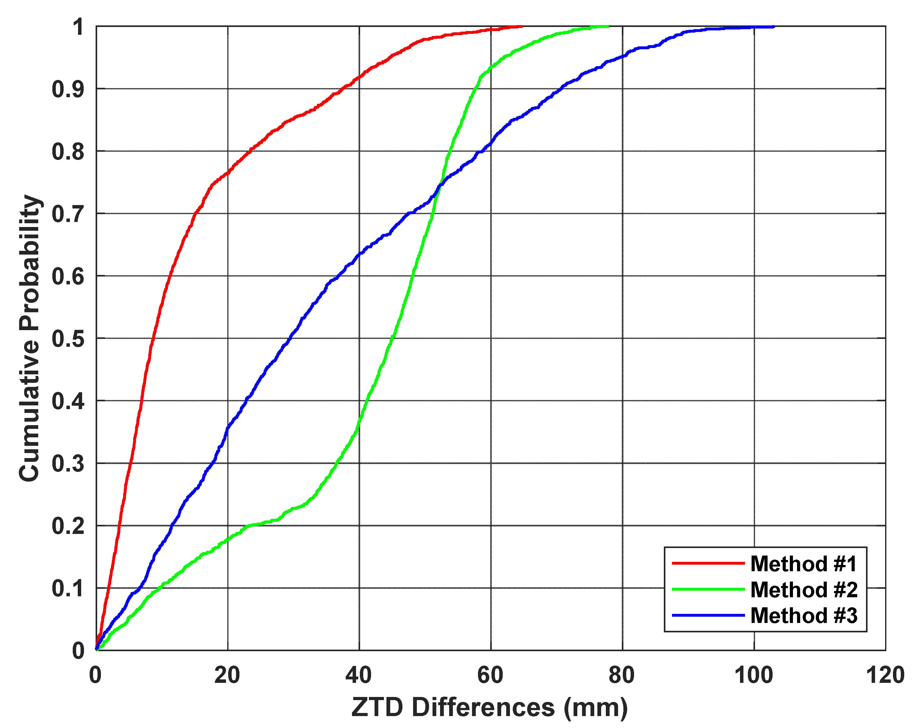
The empirical distribution functions of ZTD differences calculated by different methods are plotted in Figure 6, in which colors represent different methods indicating the percentage of each range of the ZTD differences. The maximum value of ZTD differences reached to 62, 78, and 103 mm for Methods #1–3, respectively. The percentage of ZTD differences smaller than 20 mm was 76% for Method #1; this percentage became 18% and 36% for Method #2 and Method #3, respectively. When the range was set to less than 40 mm, the percentages were increased to 92%, 37%, and 63% for Methods #1–3, respectively. These results show the advantages of the proposed model compared to the existing models.
3.3. External Accuracy Verification
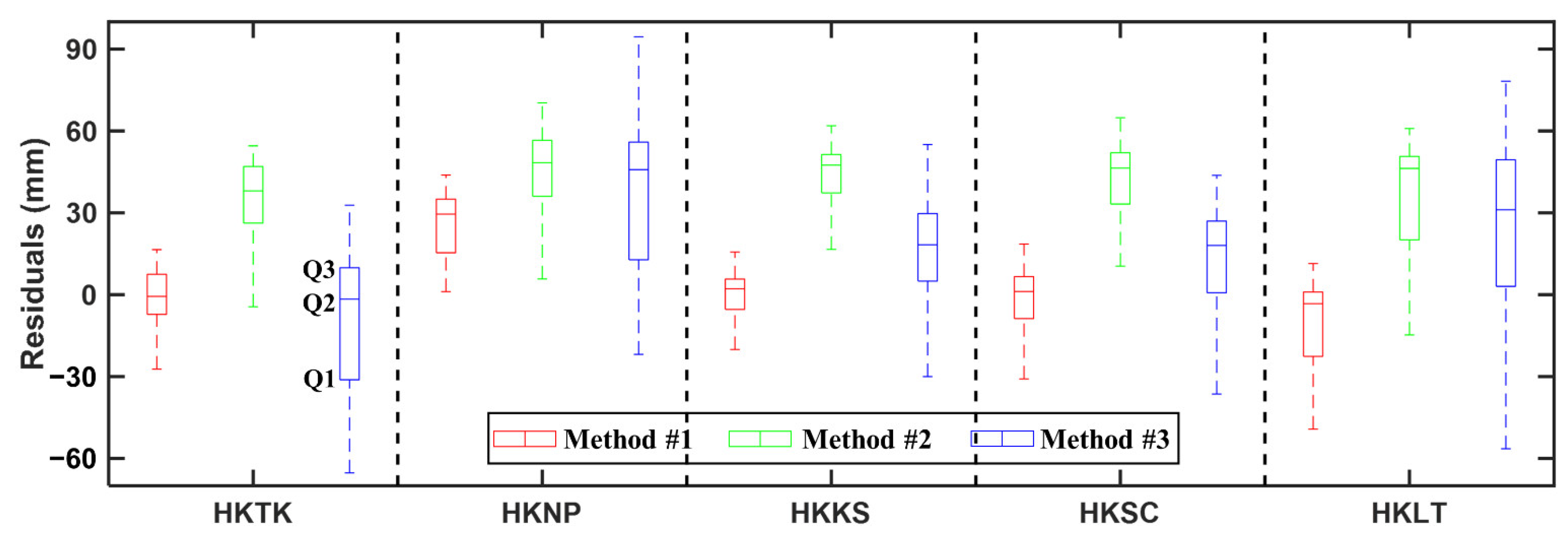
For external accuracy verification, the data from five sites, namely, HKTK, HKNP, HKKS, HKSC, and HKLT, which were not included in the ZTD modeling were used. The bias, RMSE, and CRE at each site were counted and shown in the form of a bar plot in Figure 7. It can be seen that the biases of Method #2 were all positive values, the biases of Method #3 were positive values except HKTK, while Method #1 obtained negative biases except HKNP. Note that the bias of Method #1 reached −12 mm at HKLT and 23.7 mm at HKNP, but they were still much smaller than those of the other two methods. Compared to Method #2, the proposed model had a significant improvement both in RMSE and CRE at each site, with an average improvement of 22.4 mm and 4.8 for RMSE and CRE, respectively. It also can be seen that Method #1 outperformed Method #3 at each site in terms of RMSE and CRE. The improvement at HKSC was the smallest, but it still reached 3.5 mm and 0.4 for RMSE and CRE, respectively. This identifies the fact that the proposed model improved the accuracy of the existing ZTD model, and that it can achieve the best performance in ZTD estimation.
To further illustrate the performance of the three methods in different sites, we counted the residuals between ZTD derived from the three models and the referenced ZTD, which are shown in form of boxplot in Figure 8. Box plots were used to explore the statistical characteristics of ZTD residuals, in which three characteristic values are shown. Q1 and Q3 located at the bottom and top of the box represent the first and third quartiles, respectively. The interquartile range, defined as the difference between Q3 and Q1, reflects the discreteness of a set of data. The second quartile (Q2) was located inside the box, representing the median value. At each site, the length of the box and the range of bound in Method #1 (in red) were smaller than those of other two methods (in blue and green), indicating better residual distribution using the proposed model. In this verification, Method #1 had best performance, with the median of residuals being −0.6, 29.5, 2.2, 1.2, and −3.3 mm, and 50% of the residuals were concentrated in the range of −7.2 to 7.5, 15.4 to 35.0, −5.4 to 5.7, −8.8 to 6.6, and −22.6 to 1.0 mm for HKTK, HKNP, HKKS, HKSC, and HKLT, respectively.
4. Discussion
The proposed model utilized the data from DOY of 225 to 229, 2017, during which a spell of fine weather prevailed in Hong Kong, with a ridge of high-pressure extending westwards from the Pacific to cover southeastern China. The daily rainfall was 0 mm in this period of time, which is defined as rainless days. The experiment and verification in Section 3 demonstrated that the proposed method can effectively improve the accuracy of the ZTD model in the rainless condition. It is necessary to discuss the performance of the proposed model in rainy conditions.
Thus, the period from 12 to 18 June, 2017 (DOY of 163 to 169, 2017), which covers the rainy days, was selected in this discussion. In this period of time, the maximum daily rainfall was up to 203.7 mm, the average daily rainfall was 66.8 mm, and the tropical storm and southwest monsoon made the weather remaining rainy. Similar to the ZTD modeling in rainless condition, the first 5 days of data from the 13 sites indicated by blue dots were used for ANN training to build the regional ZTD model in rainy days, and then the internal and external accuracy verifications were conducted. As most of the sites lacked measured meteorological data such as relative humidity, in this section, we mainly compare the accuracy of the two models without measured meteorological quantities, namely, Method #1 and Method #2.
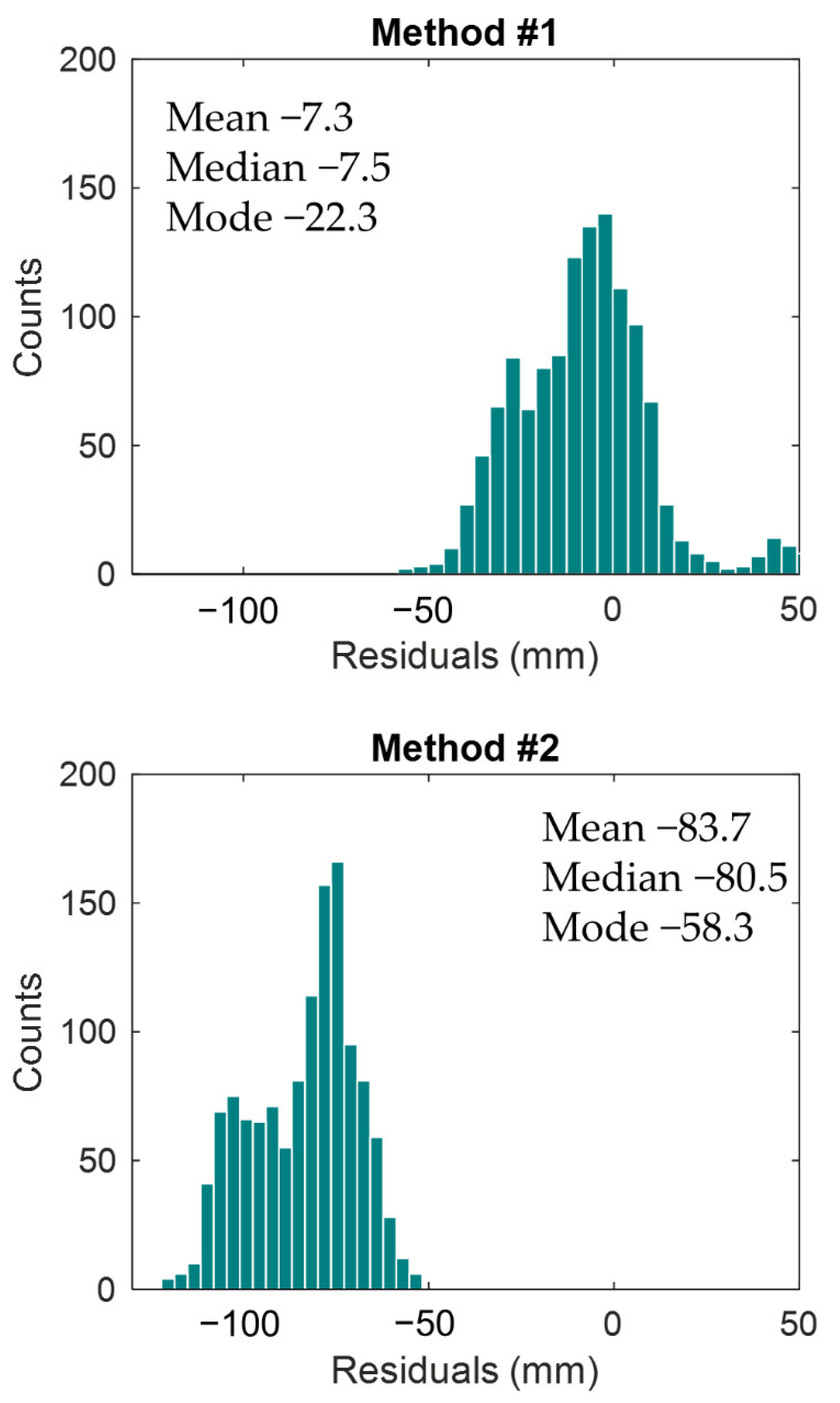
Similar to Figure 5, the RMSE, bias, as well as CRE of the 13 GNSS sites used in ZTD modelling were mapped, as shown in Figure 9, showing the internal accuracy of Methods #1 and #2 in rainy conditions. It was observed that the three statistical values obtained by the two methods did not change much at different sites, indicating that they both had stable performance in rainy days. From the values represented by the colors, the result of the GPT3 model was far worse than the proposed model. It is particularly visible that Method #2 showed negative bias at all sites, which is opposite to its bias in rainless conditions. This is most likely due to the fact that GPT3 model cannot estimate the increase in wet delay caused by the increasing water vapor in rainy days, which makes its ZTD estimates smaller. In addition, the three statistical quantities of Method #2 in rainy conditions were much larger than those in rainless conditions, showing that the accuracy of GPT3 model was affected by weather condition. Specifically, Table 3 listed the mean bias, RMSE, and CRE as well as their minimum and maximum values for the two methods in rainy conditions. The mean and maximum value of bias, RMSE, and CRE were −83.7/−89.4 mm, 84.8/90.4 mm, and 39.2/47.1 for Method #2, respectively. Compared to those in rainless conditions, the three mean values obtained by Method #2 in rainy conditions increased by 43.8 mm, 41 mm, and 33.1. However, Method #1 still obtained accurate results similar to rainless conditions, in which the mean and maximum value of bias, RMSE, and CRE were −7.3/−20.3 mm, 19.9/31.3 mm, and 1.8/3.0, respectively, indicating that the proposed model can improve the accuracy of GPT3 model under different weather conditions.
These five sites not adopted in ZTD modeling were utilized to assess the external accuracy of the two methods in rainy conditions, the detailed statistical results are listed in Table 3, in which the results of rainless condition are also shown for further comparison. Obviously, Method #2 had significant differences in the accuracy of ZTD estimation in rainless and rainy conditions, mainly in the following two aspects: (1) the biases of rainless days were positive and those of rainy days were negative, indicating that the ZTD estimated by GPT3 model in rainless conditions was relatively large while the estimate ZTD value was relatively small in rainy conditions; (2) the mean bias and RMSE of rainless days were 38.9 and 43.0 mm, respectively, while for rainy days, the values reached 82.2 and 83.3 mm, having an increase of 53% and 48%, respectively. Method #1 achieved ZTD estimation with high accuracy both in rainy and rainless days, with the mean bias and RMSE being 0.4/20.6 and −0.8/21.2 mm, respectively. For the three statistical values in this table, Method #1 had an improvement of 38.5 mm/22.4 mm/4.8 and 81.4 mm/62.1 mm/36.9 over Method #2 in different weather conditions. These illustrate again that the proposed model can effectively solve the above−mentioned defect that the accuracy of GPT3 model is affected by weather conditions.
It is particularly visible from Table 4 that the proposed model performed relatively poor at HKNP both in rainless and rainy conditions, with the three statistical values being 23.7 mm/31.6 mm/2.3 and 28.5 mm/32.0 mm/5.3, respectively. In particular, HKNP was the only site with positive bias and was 11 mm/1.0 and 10.8 mm/2.8 larger than the average RMSE and CRE in rainless and rainy days, respectively. The heights of all GNSS sites of SatRef were counted, and we found that the height of HKNP reached 350.7 m, which was 270 m higher than the average height of 80.7 m of the 13 modelling sites. This was probably one of the reasons why the proposed method did not perform well in HKNP. The phenomenon mentioned above did not appear in Method #2, since the influence of elevation was considered by the GPT3 model when calculating the meteorological parameters. Thus, the height of site could also be used as input parameters in the proposed model to explore whether the accuracy of the model will be further improved.
Further, the histogram of ZTD residuals, namely, the values of subtracting the GNSS_ZTD from model derived ZTD in terms of the mean, median, and mode values are shown in Figure 10. The three indicators were −7.3, −7.5, and −22.3 mm for the proposed model, which were better than those of the GPT3 model. From the histogram, the residuals of the proposed model are shown to be concentrated around zero and the maximum and minimum values reached around 50 and −50 mm, respectively, while the residuals of the GPT3 model were smaller than −50 mm and the minimum value reached −120 mm. The percentage of residuals in the range of −20 to 20 mm accounted for 70% in Method #1, while more than 51% residuals of Method #2 were smaller than −80 mm. These illustrate again that the GPT3 model had an obvious systematic deviation, and the proposed method can effectively improve this defect.
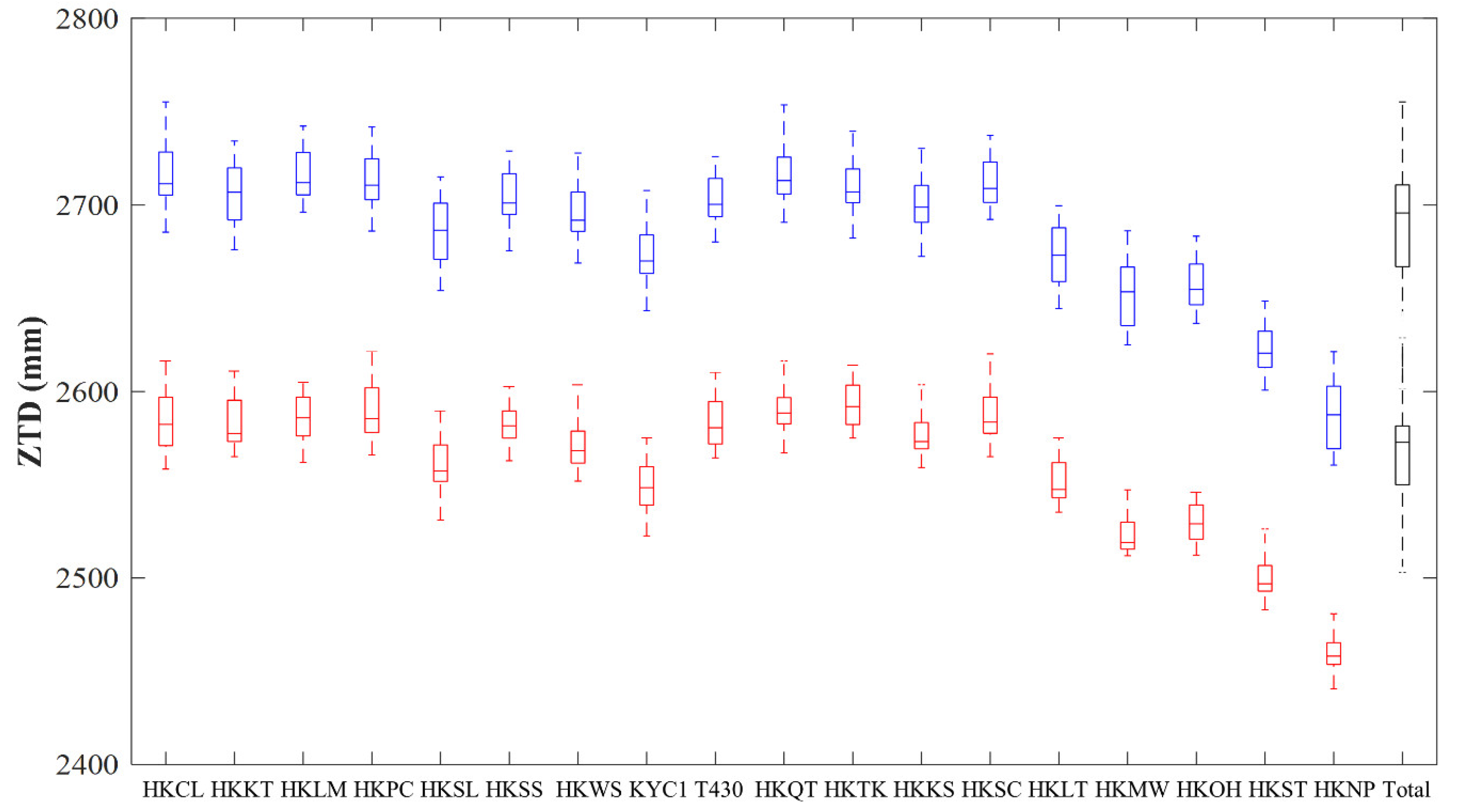
From the above comparison of the results between rainless and rainy weather conditions, we found that the results of Method #2 on rainy days were far worse than those on rainless days. This was because the spherical harmonics or trigonometric functions were used to characterize the annual and semiannual changes in parameters to estimate ZTD by empirical model. It is still difficult for this type of model to describe the variation and changes of ZTD at a certain moment, even if the model considered the diurnal changes. Further, the GNSS_ZTD, namely, the ZTD derived from GNSS data, in each GNSS site during the two periods were collected and counted. In Figure 11, the horizontal and vertical axes denote GNSS sites and GNSS_ZTD values, respectively. As expected, the values of ZTD on rainy days (blue) at each site were larger than those of rainless days (red), and the fluctuation of ZTD on rainy days was even larger from the spacings between the different parts of the box. When comparing all the ZTD data for different weather conditions, namely, the black plots, we found that the ZTD during the rainy period was relatively unstable and had a wider range of changes. Thus, the empirical models, such as GPT3 model, had worse performance of ZTD estimation in rainy conditions with more frequent ZTD fluctuations. The proposed model effectively considered the changes and variations of ZTD at a certain moment by making full use of GNSS_ZTD, eliminated the differences in ZTD estimation under different weather conditions, and improved the accuracy of existing empirical ZTD models.
5. Conclusions
It is crucial to achieve ZTD estimation with high accuracy for GNSS positioning and precipitable water vapor retrieval, especially for the sites not equipped with meteorological sensors or not collocated with weather stations. To improve the accuracy of the existing empirical model (GPT3 model) in regional ZTD estimation, we established a new regional ZTD model based on GPT3 and ANN. The proposed model made full use of the ZTD calculated from regional GNSS data and the corresponding ZTD estimated by GPT3 model, and adopted the ANN to construct the correlation between GPT3_ZTD and GNSS_ZTD.
Using the GNSS data from SatRef, we developed the new regional ZTD model for Hong Kong. Numerical results, namely, bias, RMSE, and CRE showed that the proposed model had a better performance in ZTD estimation compared with the Saastamoinen ZTD model and GPT3 model. Specifically, the proposed model achieved RMSE of 19.4 mm in the internal accuracy verification in rainless condition, which were 24.4 and 20.6 mm smaller than the parameter ZTD model and empirical model, having approximately 56% and 52% improvements over them, respectively. The amount and percentage of RMSE improvement by the proposed model also reached 22.4/52% and 12.1/37% over the other two existing models, respectively, in the external accuracy verification. For the discussion on rainy conditions, the proposed model outperformed the GPT3 model, having better statistical values, whose bias, RMSE, and CRE were −0.8 mm, 21.2 mm, and 2.5, respectively.
There are different performances in ZTD estimation of various weather conditions for the GPT3 model, which may affect by the stability of the ZTD in the research region during the experimental period. In rainy days, the ZTD values and their fluctuations are relatively large, and it is difficult for the GPT3 model to describe the variation and changes of ZTD at a certain moment. The GPT3 model achieved a bias, RMSE, and CRE of 38.9 mm, 43.0 mm, and 6.1 in rainless conditions, but the values deteriorated to −82.2 mm, 83.3 mm, and 39.4 in rainy conditions, respectively. However, the proposed model can effectively improve this defect and can achieve good performance in different conditions.
In this study, 5 days of data from 13 GNSS sites were used to construct the regional ZTD model, providing a new idea for regional ZTD modelling with high accuracy. In the follow−up research, the influence of the number of selected sites, the distribution of selected sites, and the amount of data in the training set on the proposed regional ZTD model should be studied in detail.
Author Contributions
Conceptualization, F.Y. and J.G.; Data curation, C.Z., Y.L. and J.L.; Formal analysis, F.Y.; Funding acquisition, F.Y. and J.G.; Methodology, F.Y.; Resources, C.Z., Y.L. and J.L.; Supervision, F.Y.; Validation, F.Y., C.Z. and Y.L.; Writing—original draft, F.Y.; Writing—review & editing, F.Y., J.G., C.Z., Y.L. and J.L. All authors have read and agreed to the published version of the manuscript.
Funding
This research was founded by a grant from State Key Laboratory of Resources and Environmental Information System; the Key Laboratory of Geospace Environment and Geodesy, Ministry of Education, Wuhan University (No. 19−02−08); the Guangxi Key Laboratory of Spatial Information and Geomatics (No. 19−050−11−01); the Comprehensive Remote Sensing Identification and Investigation of Geological Hazards in the Three Gorges Reservoir Area, Ministry of Natural Resources of the People’s Republic of China (No. 0733−20180876/3); and the Yueqi Young Scholars Program of China University of Mining and Technology at Beijing.
Data Availability Statement
The datasets generated and analyzed during the current study are available from the corresponding author on reasonable request. The GPT3 model can be download at https://vmf.geo.tuwien.ac.at/codes/. The GNSS observation and meteorological data from Satellite Positioning Reference Station Network (SatRet) are available at https://www.geodetic.gov.hk/en/satref/satref.htm.
Acknowledgments
Thanks to the research group of Advanced Geodesy of TU Vienna and the Hong Kong Geodetic Survey Services for providing the GPT3 model and GNSS observation, and meteorological data, respectively. We thank all anonymous reviewers for their valuable, constructive, and prompt comments.
Conflicts of Interest
The authors declare no conflict of interest. The funders had no role in the design of the study; in the collection, analyses, or interpretation of data; in the writing of the manuscript; or in the decision to publish the results.
References
- Bevis, M.; Businger, S.; Herring, T.A.; Rocken, C.; Anthes, R.A.; Ware, R.H. GPS meteorology: Remote sensing of atmospheric water vapor using the global positioning system. J. Geophys. Res. Space Phys. 1992, 97, 15787–15801. [Google Scholar] [CrossRef]
- Dodson, A.H.; Shardlow, P.J.; Hubbard, L.C.M.; Elgered, G.; Jarlemark, P.O.J. Wet tropospheric effects on precise relative GPS height determination. J. Geod. 1996, 70, 188–202. [Google Scholar] [CrossRef]
- Li, W.; Yuan, Y.; Ou, J.; Li, H.; Li, Z. A new global zenith tropospheric delay model IGGtrop for GNSS applications. Chin. Sci. Bull. 2012, 57, 2132–2139. [Google Scholar] [CrossRef] [Green Version]
- Chen, P.; Ma, Y.; Liu, H.; Zheng, N. A New Global Tropospheric Delay Model Considering the Spatiotemporal Variation Characteristics of ZTD with Altitude Coefficient. Earth Space Sci. 2020, 7, 2019000888. [Google Scholar] [CrossRef]
- Penna, N.; Dodson, A.; Chen, W. Assessment of EGNOS Tropospheric Correction Model. J. Navig. 2001, 54, 37–55. [Google Scholar] [CrossRef] [Green Version]
- Gao, Y.; Chen, K. Performance analysis of precise point positioning using real−time orbit and clock products. J. Glob. Position Syst. 2004, 3, 95–100. [Google Scholar] [CrossRef]
- Xu, G.C. GPS: Theory, Algorithms and Applications; Springer: Berlin/Heidelberg, Germany, 2007; pp. 55–62. [Google Scholar]
- Zumberge, J.F.; Heflin, M.B.; Jefferson, D.C.; Watkins, M.M.; Webb, F.H. Precise point positioning for the efficient and robust analysis of GPS data from large networks. J. Geophys. Res. Space Phys. 1997, 102, 5005–5017. [Google Scholar] [CrossRef] [Green Version]
- Karabatić, A.; Weber, R.; Haiden, T. Near real−time estimation of tropospheric water vapour content from ground based GNSS data and its potential contribution to weather now−casting in Austria. Adv. Space Res. 2011, 47, 1691–1703. [Google Scholar] [CrossRef]
- Zheng, F.; Lou, Y.; Gu, S.; Gong, X.; Shi, C. Modeling tropospheric wet delays with national GNSS reference network in Chi−na for BeiDou precise point positioning. J. Geod. 2018, 92, 545–560. [Google Scholar] [CrossRef]
- Duan, J.P.; Bevis, M.; Fang, P.; Bock, Y.; Chiswell, S.; Businger, S.; Rocken, C.; Solheim, F.; Van, H.T.; Ware, R.; et al. GPS meteorology: Direct estimation of the absolute value of precipitable water. J. Appl. Meteorol. 1996, 35, 830–838. [Google Scholar] [CrossRef] [Green Version]
- Liou, Y.-A.; Huang, C.-Y.; Teng, Y.-T. Precipitable water observed by ground−based GPS receivers and microwave radiometry. Earth Planets Space 2000, 52, 445–450. [Google Scholar] [CrossRef] [Green Version]
- Liou, Y.A.; Teng, Y.T.; Van, H.T.; Li, J. Comparison of precipitable water observations in the near tropics by GPS, microwave radiometer, and radiosondes. J. Appl. Meteor. 2001, 40, 5–15. [Google Scholar] [CrossRef]
- Hopfield, H.S. Two−quartic tropospheric refractivity profile for correcting satellite data. J. Geophys. Res. Space Phys. 1969, 74, 4487–4499. [Google Scholar] [CrossRef]
- Saastamoinen, J. Atmospheric Correction for the Troposphere and Stratosphere in Radio Ranging Satellites. Geophys. Monogr. Ser. 2013, 15, 247–251. [Google Scholar] [CrossRef]
- Black, H.D.; Eisner, A. Correcting satellite Doppler data for tropospheric effects. J. Geophys. Res. Space Phys. 1984, 89, 2616–2626. [Google Scholar] [CrossRef]
- Li, L.; Xu, Y.; Yan, L.; Wang, S.; Liu, G.; Liu, F. A Regional NWP Tropospheric Delay Inversion Method Based on a General Regression Neural Network Model. Sensors 2020, 20, 3167. [Google Scholar] [CrossRef]
- Yang, L.; Gao, J.; Zhu, D.; Zheng, N.; Li, Z. Improved Zenith Tropospheric Delay Modeling Using the Piecewise Model of Atmospheric Refractivity. Remote Sens. 2020, 12, 3876. [Google Scholar] [CrossRef]
- Collins, J.P.; Langley, R.B. A Tropospheric Delay Model for the User of the Wide Area Augmentation System; Department of Geodesy and Geomatics Engineering, University of New Brunswick: Fredericton, NB, Canada, 1997. [Google Scholar]
- Ueno, M.; Hoshinoo, K.; Matsunaga, K.; Kawai, M.; Nakao, H.; Langley, R.B.; Bisnath, S.B. Assessment of atmospheric delay correction models for the Japanese MSAS. In Proceedings of the 14th International Technical Meeting of the Satellite Division of The Institute of Navigation (ION GPS 2001), Salt Lake City, UT, USA, 11–14 September 2001; pp. 2341–2350. [Google Scholar]
- Leandro, R.F.; Santos, M.C.; Langley, R.B. A North America Wide Area Neutral Atmosphere Model for GNSS Applications. Navigation 2009, 56, 57–71. [Google Scholar] [CrossRef]
- Leandro, R.F.; Langley, R.B.; Santos, M.C. UNB3m_pack: A neutral atmosphere delay package for radiometric space tech−niques. GPS Solut. 2008, 12, 65–70. [Google Scholar] [CrossRef]
- Krueger, E.; Schueler, T.; Hein, G.W.; Martellucci, A.; Blarzino, G. Galileo Tropospheric Correction Approaches Developed within GSTB−V1. Proc. ENC−GNSS, 16–19, Rotterdam, The Netherlands. 2004. Available online: https://www.researchgate.net/profile/Torben_Schueler/publication/228730717_Galileo_Tropospheric_Correction_Approaches_Developed_within_GSTB−V1/links/09e4150880fbbbaca7000000.pdf (accessed on 1 January 2021).
- Krueger, E.; Schueler, T.; Arbesser-Rastburg, B. The Standard Tropospheric Correction Model for the European Satellite Navi−Gation System Galileo, Proc. General Assembly URSI, New Delhi, India. 2005. Available online: https://www.researchgate.net/profile/Bertram_Arbesser−Rastburg/publication/252717445_THE_STANDARD_TROPOSPHERIC_CORRECTION_MODEL_FOR_THE_EUROPEAN_SATELLITE_NAVIGATION_SYSTEM_GALILEO/links/00b4952c318413b26d000000/THE−STANDARD−TROPOSPHERIC−CORRECTION−MODEL−FOR−THE−EUROPEAN−SATELLITE−NAVIGATION−SYSTEM−GALILEO.pdf (accessed on 1 January 2021).
- Schüler, T. The TropGrid2 standard tropospheric correction model. GPS Solut. 2013, 18, 123–131. [Google Scholar] [CrossRef]
- Yao, Y.; He, C.; Zhang, B. A new global zenith tropospheric delay model GZTD. Chin. J. Geophys. 2013, 56, 2218–2227. [Google Scholar] [CrossRef]
- Yao, Y.; Hu, Y.; Yu, C.; Zhang, B.; Guo, J. An improved global zenith tropospheric delay model GZTD2 considering diurnal variations. Nonlinear Process. Geophys. 2016, 23, 127–136. [Google Scholar] [CrossRef] [Green Version]
- Mateus, P.; Catalao, J.; Mendes, V.; Nico, G. An ERA5−based hourly global pressure and temperature (HGPT) model. Remote Sens. 2020, 12, 1098. [Google Scholar] [CrossRef] [Green Version]
- Li, W.; Yuan, Y.; Ou, J.; He, Y. IGGtrop_SH and IGGtrop_rH: Two Improved Empirical Tropospheric Delay Models Based on Vertical Reduction Functions. IEEE Trans. Geosci. Remote Sens. 2018, 56, 5276–5288. [Google Scholar] [CrossRef]
- Sun, J.; Wu, Z.; Yin, Z.; Ma, B. A simplified GNSS tropospheric delay model based on the nonlinear hypothesis. GPS Solut. 2017, 21, 1735–1745. [Google Scholar] [CrossRef]
- Charoenphon, C.; Satirapod, C. Improving the accuracy of real−time precipitable water vapour using country−wide meteorological model with precise point positioning in Thailand. J. Spat. Sci. 2020, 1–17. [Google Scholar] [CrossRef]
- Chen, J.; Wang, J.; Wang, A.; Ding, J.; Zhang, Y. SHAtropE—A Regional Gridded ZTD Model for China and the Surrounding Areas. Remote Sens. 2020, 12, 165. [Google Scholar] [CrossRef] [Green Version]
- Böhm, J.; Möller, G.; Schindelegger, M.; Pain, G.; Weber, R. Development of an improved empirical model for slant delays in the troposphere (GPT2w). GPS Solut. 2015, 19, 433–441. [Google Scholar] [CrossRef] [Green Version]
- Landskron, D.; Boehm, J. VMF3/GPT3: Refined discrete and empirical troposphere mapping functions. J. Geod. 2018, 92, 349–360. [Google Scholar] [CrossRef]
- Liu, J.; Chen, X.; Sun, J.; Liu, Q. An analysis of GPT2/GPT2w+Saastamoinen models for estimating zenith tropospheric delay over Asian area. Adv. Space Res. 2017, 3, 824–832. [Google Scholar] [CrossRef]
- Chen, W.; Gao, C.; Pan, S. Assessment of GPT2 empirical troposphere model and application analysis in precise point positioning. In Proceedings of the China Satellite Navigation Conference (CSNC) 2014 Proceedings: Volume II, Nanjing, China, 21–23 May 2014; Lecture Notes in Electrical Engineering. Volume 304, pp. 451–463. [Google Scholar]
- Ding, J.; Chen, J. Assessment of empirical troposphere model GPT3 based on NGL’s global troposphere products. Sensors 2020, 20, 3631. [Google Scholar] [CrossRef]
- Snav, N.; Soler, T. Continuously operating reference station (CORS): History, applications and future enhancements. J. Surv. Eng. 2008, 4, 95. [Google Scholar]
- Riccardi, U.; Tammaro, U.; Capuano, P. Evaluation of the atmospheric precipitable water at local scale during extreme weather using ground−based CGPS measurements. In Proceedings of the 2013 IEEE Workshop on Environmental, Energy and Structural Monitoring System, EESMS 2013, Trento, Italy, 11–12 September 2013; pp. 1–4. [Google Scholar]
- Boehm, J.; Heinkelmann, R.; Schuh, H. Short Note: A global model of pressure and temperature for geodetic applications. J. Geod. 2007, 81, 679–683. [Google Scholar] [CrossRef]
- Lagler, K.; Schindelegger, M.; Böhm, J.; Krásná, H.; Nilsson, T. GPT2: Empirical slant delay model for radio space geodetic techniques. Geophys. Res. Lett. 2013, 40, 1069–1073. [Google Scholar] [CrossRef] [PubMed] [Green Version]
- Askne, J.; Nordius, H. Estimation of tropospheric delay for microwaves from surface weather data. Radio Sci. 1987, 22, 379–386. [Google Scholar] [CrossRef]
- Wang, J.; Ji, H.; Wang, Q.G.; Li, H.; Qian, X.; Li, F.; Yang, M. Prediction of size−fractionated airborne particle−bound metals using MLR, BP−ANN and SVM analyses. Chemosphere 2017, 180, 513–522. [Google Scholar]
- Yang, S.; Feng, Q.; Liang, T.; Liu, B.; Zhang, W.; Xie, H. Modeling grassland above−ground biomass based on artificial neural network and remote sensing in the Three−River Headwaters Region. Remote Sens. Environ. 2018, 204, 448–455. [Google Scholar] [CrossRef]
- Feng, Y.; Zhang, W.; Sun, D.; Zhang, L. Ozone concentration forecast method based on genetic algorithm optimized back propagation neural networks and support vector machine data classification. Atmos. Environ. 2011, 45, 1979–1985. [Google Scholar] [CrossRef]
- Specht, D. A general regression neural network. IEEE Trans. Neural Netw. 1991, 2, 568–576. [Google Scholar] [CrossRef] [Green Version]
- Cui, Y.; Long, D.; Hong, Y.; Zeng, C.; Zhou, J.; Han, Z.; Liu, R.; Wan, W. Validation and reconstruction of FY−3B/MWRI soil moisture using an artificial neural network based on reconstructed MODIS optical products over the Tibetan Plateau. J. Hydrol. 2016, 543, 242–254. [Google Scholar] [CrossRef]
- Yang, T.; Wan, W.; Sun, Z.; Liu, B.; Li, S.; Chen, X. Comprehensive evaluation of using TechDemoSat−1 and CYGNSS data to estimate soil moisture over mainland China. Remote Sens. 2020, 12, 1699. [Google Scholar] [CrossRef]
- Boehm, J.; Niell, A.; Tregoning, P.; Schuh, H. Global Mapping Function (GMF): A new empirical mapping function based on numerical weather model data. Geophys. Res. Lett. 2006, 33, 7. [Google Scholar] [CrossRef] [Green Version]
- Yao, Y.; Zhao, Q. Maximally using GPS observation for water vapor tomography. IEEE Trans. Geosci. Remote Sens. 2016, 54, 7185–7196. [Google Scholar] [CrossRef]
- Chen, Q.; Song, S.; Heise, S.; Liou, Y.; Zhu, W.; Zhao, J. Assessment of ZTD derived from ECMWF/NCEP data with GPS ZTD over China. GPS Solut. 2011, 15, 415–425. [Google Scholar] [CrossRef]
- Hofstra, N.; Haylock, M.; New, M.; Jones, P.; Frei, C. Comparison of six methods for the interpolation of daily, European climate data. J. Geophys. Res. 2008, 113, D21110. [Google Scholar] [CrossRef] [Green Version]
- Serrano, S.M.V.; Sánchez, M.; Ángel, S.; Cuadrat, J.M. Comparative analysis of interpolation methods in the middle Ebro Valley (Spain): Application to annual precipitation and temperature. Clim. Res. 2003, 24, 161–180. [Google Scholar] [CrossRef] [Green Version]
Figure 1.
The diagram of artificial neural network (ANN).

Figure 2.
The distribution of the global navigation satellite system (GNSS) stations in Hong Kong (blue dots denote training sites and red dots represent test sites in ANN).
Figure 2.
The distribution of the global navigation satellite system (GNSS) stations in Hong Kong (blue dots denote training sites and red dots represent test sites in ANN).

Figure 3.
Flowchart of the establishment of regional zenith tropospheric delay (ZTD) model based on global pressure and temperature 3 (GPT3) and ANN.
Figure 3.
Flowchart of the establishment of regional zenith tropospheric delay (ZTD) model based on global pressure and temperature 3 (GPT3) and ANN.

Figure 4.
Histogram of the residuals (upper panel) and linear regression (lower panel) for the training and validation set in ANN.
Figure 4.
Histogram of the residuals (upper panel) and linear regression (lower panel) for the training and validation set in ANN.

Figure 5.
Map showing root mean square error (RMSE), bias, and compound relative error (CRE) at the 13 GNSS sites for the three methods.
Figure 5.
Map showing root mean square error (RMSE), bias, and compound relative error (CRE) at the 13 GNSS sites for the three methods.

Figure 6.
The empirical distribution functions of the ZTD differences for the three methods.

Figure 7.
Histogram of bias, RMSE, and CRE at five sites for the three methods.

Figure 8.
Box and Whisker of the residuals for the three methods.

Figure 9.
Map showing RMSE, bias, and CRE at the 13 GNSS sites for the two methods in rainy conditions.
Figure 9.
Map showing RMSE, bias, and CRE at the 13 GNSS sites for the two methods in rainy conditions.

Figure 10.
Histogram of the residuals between the ZTD derived from models (upper for Method #1 and lower for Method #2) and the reference ZTD.
Figure 10.
Histogram of the residuals between the ZTD derived from models (upper for Method #1 and lower for Method #2) and the reference ZTD.

Figure 11.
Box and Whisker of the observed ZTD in each site during the period of rainless and rainy days. Blue for the rainy conditions and red for the rainless conditions, and black for the combination of the two weather conditions.
Figure 11.
Box and Whisker of the observed ZTD in each site during the period of rainless and rainy days. Blue for the rainy conditions and red for the rainless conditions, and black for the combination of the two weather conditions.


Table 1.
The coordinates of GNSS stations in Hong Kong.
| Sites | Latitude | longitude | Ellipsoidal Height (m) |
|---|---|---|---|
| HKCL | 22.30 | 113.91 | 7.71 |
| HKKS | 22.37 | 114.31 | 44.72 |
| HKKT | 22.44 | 114.07 | 34.58 |
| HKLM | 22.22 | 114.12 | 8.55 |
| HKLT | 22.42 | 114.00 | 125.92 |
| HKMW | 22.26 | 114.00 | 194.95 |
| HKNP | 22.25 | 113.89 | 350.67 |
| HKOH | 22.25 | 114.23 | 166.40 |
| HKPC | 22.28 | 114.04 | 18.13 |
| HKQT | 22.29 | 114.21 | 5.18 |
| HKSC | 22.32 | 114.14 | 20.24 |
| HKSL | 22.37 | 113.93 | 95.30 |
| HKSS | 22.43 | 114.27 | 38.71 |
| HKST | 22.40 | 114.18 | 258.70 |
| HKTK | 22.55 | 114.22 | 22.53 |
| HKWS | 22.43 | 114.34 | 63.79 |
| KYC1 | 22.28 | 114.08 | 116.38 |
| T430 | 22.49 | 114.14 | 41.32 |
Table 2.
Summary of the performance evaluation of different methods for internal accuracy verification.
Table 2.
Summary of the performance evaluation of different methods for internal accuracy verification.
| Bias (mm) | RMSE (mm) | CRE | |
|---|---|---|---|
| Method #1 | −7.7 [−15.7 1.3] | 19.4 [14.7 26.2] | 1.1 [0.9 1.6] |
| Method #2 | 39.9 [35.7 47.1] | 43.8 [40.1 51.4] | 6.1 [3.9 9.2] |
| Method #3 | 19.6 [−41.1 60.0] | 40.0 [20.9 64.7] | 5.5 [1.2 12.4] |
Table 3.
Summary of the performance evaluation for the two methods in rainy condition.
| Bias (mm) | RMSE (mm) | CRE | |
|---|---|---|---|
| Method #1 | −7.3 [−20.3 −1.1] | 19.9 [14.0 31.3] | 1.8 [1.0 3.0] |
| Method #2 | −83.7 [−81.4 −89.4] | 84.8 [82.4 90.4] | 39.2 [26.9 47.1] |
Table 4.
Statistical results of the external accuracy verification for the two methods in rainless and rainy conditions.
Table 4.
Statistical results of the external accuracy verification for the two methods in rainless and rainy conditions.
| − | Weather | Site | Bias (mm) | RMSE (mm) | CRE |
|---|---|---|---|---|---|
| Method #1 | Rainless conditions | HKTK | −2.0 | 14.8 | 0.9 |
| HKNP | 23.7 | 31.6 | 2.3 | ||
| HKKS | −1.6 | 13.4 | 0.9 | ||
| HKSC | −6.0 | 20.3 | 1.0 | ||
| HKLT | −12.0 | 22.7 | 1.1 | ||
| average | 0.4 | 20.6 | 1.3 | ||
| Rainy conditions | HKTK | −20.7 | 20.0 | 2.2 | |
| HKNP | 28.5 | 32.0 | 5.3 | ||
| HKKS | −5.0 | 14.8 | 1.1 | ||
| HKSC | −12.5 | 20.9 | 2.7 | ||
| HKLT | −4.3 | 18.4 | 1.2 | ||
| average | −0.8 | 21.2 | 2.5 | ||
| Method #2 | Rainless conditions | HKTK | 34.8 | 37.9 | 6.2 |
| HKNP | 42.2 | 47.0 | 5.1 | ||
| HKKS | 42.3 | 44.4 | 10.3 | ||
| HKSC | 39.0 | 43.7 | 4.8 | ||
| HKLT | 36.3 | 42.0 | 3.9 | ||
| average | 38.9 | 43.0 | 6.1 | ||
| Rainy conditions | HKTK | −81.9 | 83.0 | 37.7 | |
| HKNP | −80.4 | 81.7 | 34.9 | ||
| HKKS | −81.6 | 82.8 | 35.5 | ||
| HKSC | −83.6 | 84.6 | 44.0 | ||
| HKLT | −83.3 | 84.3 | 44.8 | ||
| average | −82.2 | 83.3 | 39.4 |
Publisher’s Note: MDPI stays neutral with regard to jurisdictional claims in published maps and institutional affiliations. |
© 2021 by the authors. Licensee MDPI, Basel, Switzerland. This article is an open access article distributed under the terms and conditions of the Creative Commons Attribution (CC BY) license (http://creativecommons.org/licenses/by/4.0/).
Share and Cite
MDPI and ACS Style
Yang, F.; Guo, J.; Zhang, C.; Li, Y.; Li, J. A Regional Zenith Tropospheric Delay (ZTD) Model Based on GPT3 and ANN. Remote Sens. 2021, 13, 838. https://doi.org/10.3390/rs13050838
AMA Style
Yang F, Guo J, Zhang C, Li Y, Li J. A Regional Zenith Tropospheric Delay (ZTD) Model Based on GPT3 and ANN. Remote Sensing. 2021; 13(5):838. https://doi.org/10.3390/rs13050838
Chicago/Turabian StyleYang, Fei, Jiming Guo, Chaoyang Zhang, Yitao Li, and Jun Li. 2021. "A Regional Zenith Tropospheric Delay (ZTD) Model Based on GPT3 and ANN" Remote Sensing 13, no. 5: 838. https://doi.org/10.3390/rs13050838
Note that from the first issue of 2016, this journal uses article numbers instead of page numbers. See further details here.