2.1 Transition probabilities using TAMS

We consider finite-dimensional dynamical systems described by stochastic differential equations (SDEs) of the following form:

where X_t∈ℝⁿ and $\mathit{F}:{\mathbb{R}}^n\to {\mathbb{R}}^n$ is the drift field. The noise term W_t∈ℝ^m consists of m independent Wiener processes, with the matrix $\mathbf{G}:{\mathbb{R}}^n\times {\mathbb{R}}^m$ being the noise matrix.

A prominent example of such a system is a model of a free particle moving in a two-dimensional double-well potential (with $n=m=\mathrm{2}$). The drift term in the time-evolution equation for the variables x and y is in this case

where V(x,y) represents the potential (Fig. 1a). In the deterministic case (i.e. G=0), the stable steady states of the system are ${\mathit{X}}_A=(-\mathrm{1},\mathrm{0})$ and ${\mathit{X}}_B=(+\mathrm{1},\mathrm{0})$, while the unstable steady state is ${\mathit{X}}_C=(\mathrm{0},\mathrm{0})$. Without fluctuations, a particle starting in X_A stays in X_A. However, because of the presence of unresolved processes (such as thermal fluctuations), modelled by the noise term in the SDE, the particle can move away from X_A and in some cases make the transition to the state X_B. An example of such a transition is shown in Fig. 1b.

Figure 1(a) Iso-potential contours corresponding to the double-well potential (Eq. 2). The two stable steady states ${\mathit{X}}_A=(-\mathrm{1},\mathrm{0})$ and ${\mathit{X}}_B=(+\mathrm{1},\mathrm{0})$ are marked with a filled circle and a cross, respectively. The saddle ${\mathit{X}}_C=(\mathrm{0},\mathrm{0})$ is indicated by a circle. (b) Example of a noise-induced transition from X_A to X_B for a particle moving in the double-well potential in (a). The noise matrix in the general SDE (1) is chosen as G=σI, with σ=0.32. The red circle denotes an arbitrarily defined target set B.

Download

The transition probability that a trajectory starting in X_A reaches a neighbourhood B around X_B before time T is indicated by $P({\mathit{\tau }}_B<T|{\mathit{X}}_{\mathrm{0}}={\mathit{X}}_A)$. Here, τ_B denotes the stopping time associated with reaching B. The TAMS algorithm is based on a selection and mutation process of discarding and branching trajectories, which are ranked according to a score function $\mathit{\varphi }:{\mathbb{R}}^n\times \mathbb{R}\to \mathbb{R}$. For a given state $(\mathit{X},t)\in {\mathbb{R}}^n\times \mathbb{R}$, ϕ(X,t) is supposed to measure how likely it is to start in (X,t) and reach B before time T. As a consequence, if the choice of score function is successful, the probability that a trajectory reaches the target set B keeps increasing at each iteration of the algorithm, which is why this method is more efficient than brute-force techniques. A visual representation of the algorithm is given in Fig. 2 and a step-by-step description is provided in Appendix A (more details can be found in Lestang et al., 2018).

Figure 2Illustration of the TAMS algorithm. First, simulate N trajectories starting in X_A (N=3 blue trajectories in the figure). The trajectories are ranked according to their score ϕ_i, which is the maximum value of the score function ϕ along the trajectory. Then, at each iteration, the trajectory with the lowest score (1 in the figure, with score ϕ₁) is discarded. It is replaced by picking a trajectory uniformly at random from the other ones (2 in the figure), then computing the earliest position at which it reaches a higher score than the discarded trajectory (orange dot) and finally using this position as the branching point for the new trajectory (1^′). This is repeated until all the trajectories reach B or the number of iterations reaches a predefined limit.

Download

2.2 Score functions

Consider a general SDE (1) and two stable states X_A and X_B of the corresponding deterministic system. The TAMS algorithm (see Appendix A) needs a score function to be defined, which allows us to rank trajectories and select the ones to discard. The optimal score function ϕ_com(X,t), i.e. the score function that minimises the variance of the probability estimator, is called the static committor. Its generic expression is given by the following conditional probability (Lestang et al., 2018):

where T is again the fixed duration of the trajectories and τ_B is the stopping time associated with reaching the target set B. In other words, ϕ_com(X,t) is the probability that a trajectory starting in X at time t reaches B before time T. This expression is quite natural because ideally, the score of (Y,s) should be higher than the score of (X,t), i.e. $\mathit{\varphi }(\mathit{X},t)\le \mathit{\varphi }(\mathit{Y},s)$, if and only if $P({\mathit{\tau }}_B<T|\mathit{X},t)\le P({\mathit{\tau }}_B<T|\mathit{Y},s)$. This condition is clearly satisfied by ϕ_com (and in fact any increasing function of ϕ_com). However, the expression given in Eq. (3) is generally unusable because it is the very quantity that we want to compute. For instance, ϕ_com(X_A,0) is precisely the transition probability that TAMS estimates. As a conditional probability of the form $P(\mathit{Y},s|\mathit{X},t)$, the committor ϕ_com(X,t) satisfies the backward Fokker–Planck equation (Lestang et al., 2018):

However, solving the backward Fokker–Planck equation in systems with many degrees of freedom is computationally unfeasible. Moreover, even if the committor is available on a grid used for the discretisation of Eq. (4), using interpolation to evaluate it during a TAMS loop can also have a prohibitive computational cost.

Bouchet et al. (2019) made use of a score function based on the distances of the state X from the starting state X_A and the destination equilibrium X_B, respectively. It is defined as

Alternatively, a Gaussian-shaped score function ϕ_gauss was proposed in Baars (2019). It is defined as

with $\mathit{\eta }\equiv \parallel {\mathit{X}}_C-{\mathit{X}}_A\parallel /\parallel {\mathit{X}}_A-{\mathit{X}}_B\parallel$. Here β∈ℝ is a parameter controlling the decay and X_C is the saddle state of the system. Due to the general expressions of ϕ_gauss and ϕ_dist, these score functions can be used in systems of any dimension.

2.3 Definition of the target set

Once the score function has been chosen, a threshold needs to be defined for the TAMS algorithm to converge, so that the occurrence of a transition can be detected. In other words, we do not expect each trajectory that undergoes a transition to reach exactly the destination equilibrium X_B, but rather a neighbourhood of it (B). The target set B can then be defined according to a level set ϕ^target of the score function ϕ:

However, different score functions ϕ and different level sets ϕ^target correspond to different target sets B, which can differ in volume and in shape. Moreover, often the level set ϕ^target is defined somewhat arbitrarily. For example, by using ϕ_gauss with target score ${\mathit{\varphi }}^{\text{target}}=\mathrm{0.85},\mathrm{0.9}$ or 0.95, we found that the average of the transition probability estimator for a two-dimensional double-well potential system (Eq. 2) can vary by up to 30 %. This may not be a concern if one only cares about the order of magnitude of the transition probability, but it will be problematic if quantitative comparisons are needed. Moreover, a poor choice of target set can lead to inaccuracies when a trajectory has a score greater than ϕ^target without actually making the transition in all the degrees of freedom. Thus, there is a need to define a canonical choice of a target set B, which needs to fundamentally address what is considered to be a noise-induced transition.

For this purpose, we use the concept of a confidence ellipsoid. This is an ellipsoidal neighbourhood around a stable equilibrium state, inside which a trajectory subject to the locally linearised dynamics stays, within a certain confidence level (Cowan, 1998).

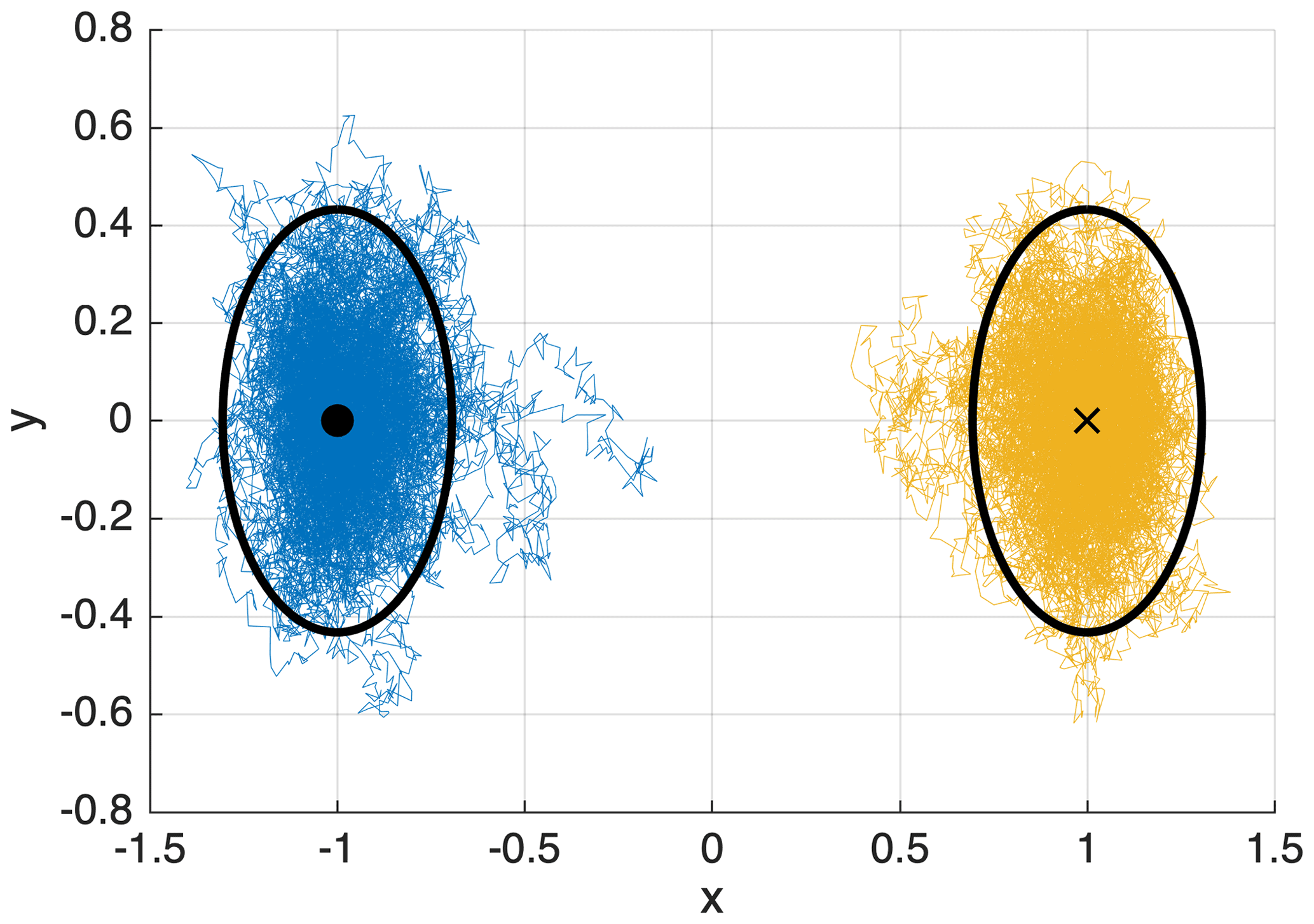
Figure 3Confidence ellipsoids for the two-dimensional double-well potential system (Eq. 2), with confidence level $\mathrm{1}-\mathit{\alpha }=\mathrm{0.95}$ and noise matrix G=0.25I, where I is the identity matrix in ℝ². Two trajectories of duration T=200 are shown: one (blue) is initialised at the initial state and one (orange) at the target state. 93 % of the points composing a trajectory are inside their corresponding ellipsoid. This is lower than the prescribed confidence level because away from the equilibrium, the first-order dynamics from which the confidence ellipsoids are derived does not hold.

Download

Consider a general SDE system given by Eq. (1). Because the drift vanishes at an equilibrium state F(X_B)=0, its first-order approximation around the equilibrium state X_B via Taylor expansion is

where $\mathbf{A}\left({\mathit{X}}_B\right)=\mathrm{\nabla }F\left({\mathit{X}}_B\right)\in {\mathbb{R}}^{n\times n}$ is the Jacobian matrix of F at X_B. Using a translation $\stackrel{\mathrm{̃}}{\mathit{X}}=\mathit{X}-{\mathit{X}}_B$, the first-order approximation of the SDE is then

Because the drift term has been linearised, this is the equation for an n-dimensional Ornstein–Uhlenbeck process. The stationary probability density function (PDF) f of the approximating process is Gaussian (Cowan, 1998) and given by

where ${\mathbf{C}}_B\in {\mathbb{R}}^{n\times n}$ is the covariance matrix of the system calculated in X_B and $\parallel .{\parallel }_{{\mathbf{C}}_B^{-\mathrm{1}}}$ the norm induced by its inverse ${\mathbf{C}}_B^{-\mathrm{1}}$, defined by $\parallel \mathit{X}{\parallel }_{{\mathbf{C}}_B^{-\mathrm{1}}}^{\mathrm{2}}\equiv {\mathit{X}}^{\top }{\mathbf{C}}_B^{-\mathrm{1}}\mathit{X}$. The covariance matrix C_B can be thought of heuristically as the matrix containing the correlations 𝔼(x_ix_j) (with $\mathit{X}=(x_{\mathrm{1}},\mathrm{\dots },x_n)$), which generalises the notion of variance in n dimensions. C_B is obtained by solving the Lyapunov equation (see Kuehn, 2012, for the full derivation):

We then define the confidence ellipsoid, which has ${\mathbf{C}}_B^{-\mathrm{1}}$ as a shape matrix, as follows:

where Q_α is the quantile of confidence level 1−α of the n-dimensional χ² distribution (Cowan, 1998), usually $\mathrm{1}-\mathit{\alpha }=\mathrm{0.95}$. The directions of symmetry of the ellipsoids are given by the eigenvectors of the covariance matrix C_B and the radii are given by the corresponding eigenvalues and the confidence level 1−α. Intuitively, the greater the eigenvalue, the more a trajectory fluctuates in the given direction.

The (1−α)-covariance ellipsoid represents the n-dimensional volume where a trajectory is confined with confidence level 1−α, provided its dynamics is well approximated by the first-order expansion at the equilibrium point. An illustration of the 0.95-confidence ellipsoid for the double-well potential is shown in Fig. 3. The confidence ellipsoid ℰ constitutes a way to meaningfully define the target set B with minimal arbitrary parameters. As shown in Fig. 3, when initialising a trajectory at X_A or X_B in the two-dimensional double-well system, it stays inside the correspondent ellipsoid with a certain confidence $\mathrm{1}-\mathit{\alpha }=\mathrm{0.95}$. In the next section, we show how to incorporate this choice of target set into the score function ϕ.

2.4 Estimating the typical transition path using histograms

The second line of improvement of the score function concerns the estimation of typical transition paths of the dynamical system. In the zero noise limit, the Freidlin–Wentzell theory of large deviations predicts that transition paths will cluster around the most probable transition path, called the instanton (Freidlin and Wentzell, 1984). On the other hand, in the finite noise regime, transition paths may deviate from the instanton. Moreover, instantons may be computationally inaccessible for systems with many degrees of freedom. Therefore, it can prove more relevant to estimate empirically the typical transition path that the system follows at a given finite noise level, which is the approach we follow here.

The idea is to first accumulate transition paths at a noise level where transitions are frequent enough (typically $p>{\mathrm{10}}^{-\mathrm{3}}$) so that any sampling method (direct Monte Carlo or TAMS with naive score functions) can be used. Then, we compute the spatial histogram of the transition paths over a discretised phase space using n-dimensional boxes. This provides the spatial distribution of the transition paths, which is concentrated around a typical transition path, reminiscent of an instanton phenomenology, which was also observed in more complex systems (Bouchet et al., 2019). From the spatial histogram, we extract a typical transition path.

The main steps of the path-finding algorithm are listed below:

• i.

  the trajectory of the typical transition path starts in the box of the histogram containing the initial state X_A;

• ii.

  the next box in this trajectory corresponds to the neighbour which has the highest nonzero histogram value but which has not already been visited by the typical transition path;

• iii.

  the algorithm stops if it reaches the box containing the target state X_B.

In addition, the full typical path estimation algorithm uses a self-correcting method to avoid dead ends when there are no valid neighbours to be the next point in the trajectory. The spirit of the path-finding algorithm is similar to the depth-first search algorithm (Cormen et al., 2009). We found that, as long as the histogram is not fragmented, i.e. there is a sufficient number of accumulated trajectories or large enough histogram bins, the algorithm converges. Possible artefacts created by this estimation include spiralling near the initial equilibrium (because of the concentric shell structure of the local probability density function, Eq. 10) and zigzagging at the histogram box size. They can both be addressed by a clean-up algorithm: starting from the first box, at each box X_j, if the trajectory goes back to one of its neighbours at a later time, with X_j+k being the latest neighbour visit, we erase the points ${\mathit{X}}_{j+\mathrm{1}},\mathrm{\dots },{\mathit{X}}_{j+k}$ from the trajectory.

In a general system, transitions induced at high noise do not necessarily follow similar transition paths at lower noise levels. However, high-noise estimates are robust as long as there is no drastic change in the behaviour of the system at an intermediate noise level, which would signal a physical phase transition in the system (Rolland and Simonnet, 2015). Moreover, we can check a posteriori if such a transition occurs by starting at high noise, gradually decrease the noise level and apply the empirical estimation of the typical path or simply compare histograms each time the noise level is decreased.

3.1 Incorporating ellipsoids in the score function

First, we apply the modified TAMS method to the two-dimensional double-well system defined by Fig. 1. As outlined in Sect. 2.3, given any score function ϕ, we want the target set $B=\mathit{\{}\mathit{X}\in {\mathbb{R}}^n\mid \mathit{\varphi }(\mathit{X})>{\mathit{\varphi }}^{\text{target}}\mathit{\}}$ to coincide with the 0.95-confidence ellipsoid ℰ associated with the equilibrium state X_B. However, because the contour levels of ϕ, in general, do not have the shape of an ellipsoid, there is no suitable choice of ϕ^target such that B coincides with ℰ. Here, we propose a general method to modify any score function ϕ so that we are able to choose the target set B to be exactly the 0.95-confidence ellipsoid ℰ of X_B.

Figure 4(a) Contour levels of the modified score function ${\stackrel{\mathrm{̃}}{\mathit{\varphi }}}_{\text{gauss}}$, for the two-dimensional double-well system represented in Fig. 1, according to the procedure described in Eq. (14). The level set ϕ^target (dotted blue line) of the former score function ϕ_gauss is tangent to the ellipsoid. The level set ${\stackrel{\mathrm{̃}}{\mathit{\varphi }}}^{\text{target}}$ (dotted red) of the modified score function ${\stackrel{\mathrm{̃}}{\mathit{\varphi }}}_{\text{gauss}}$ coincides with the ellipsoid. (b) Same plot for the score function ${\stackrel{\mathrm{̃}}{\mathit{\varphi }}}_{\text{dist}}$.

Download

We first compute the level ${\stackrel{\mathrm{̃}}{\mathit{\varphi }}}^{\text{target}}$, defined as the minimum of the score function ϕ on the confidence ellipsoid ℰ:

such that the set $\mathit{\{}\mathit{X}\in {\mathbb{R}}^n\mid \mathit{\varphi }(\mathit{X})>{\stackrel{\mathrm{̃}}{\mathit{\varphi }}}^{\text{target}}\mathit{\}}$ contains the ellipsoid ℰ and is tangent to ℰ. This can be done numerically by generating a mesh of points around X_B, then selecting the points inside ℰ by comparing their norm $\parallel \mathit{X}-{\mathit{X}}_B{\parallel }_{C_B^{-\mathrm{1}}}^{\mathrm{2}}$ with the quantile Q_α and finally computing the minimum ${\stackrel{\mathrm{̃}}{\mathit{\varphi }}}^{\text{target}}$ of ϕ on these points. Then, define the modified score function $\stackrel{\mathrm{̃}}{\mathit{\varphi }}$ in the following way:

The target set $B=\mathit{\{}\mathit{X}\in {\mathbb{R}}^n\mid \stackrel{\mathrm{̃}}{\mathit{\varphi }}(\mathit{X})>{\stackrel{\mathrm{̃}}{\mathit{\varphi }}}^{\text{target}}\mathit{\}}$ for the modified score function $\stackrel{\mathrm{̃}}{\mathit{\varphi }}$ turns out to coincide with ℰ. We apply this procedure on both the score functions ϕ_gauss and ϕ_dist, and the results for the improved score functions ${\stackrel{\mathrm{̃}}{\mathit{\varphi }}}_{\text{dist}}$ and ${\stackrel{\mathrm{̃}}{\mathit{\varphi }}}_{\text{gauss}}$ are shown in Fig. 4.

3.2 Designing a score function based on a typical transition path

In order to show how to design a score function based on a typical transition path, we consider a two-dimensional system slightly less trivial than the double-well system, i.e. a two-dimensional system with the following potential,

depicted in Fig. 5a. It consists of two energy minima at ${\mathit{X}}_A\approx (-\mathrm{5.77},\mathrm{0})$ and ${\mathit{X}}_B\approx (\mathrm{5.77},\mathrm{0})$ and a potential barrier spanning y<15 and at x=0. The dynamics is then given by the SDE (1), with drift $\mathit{F}\left({\mathit{X}}_t\right)=-\mathbf{\nabla }V\left({\mathit{X}}_t\right)$.

The dynamics of the system is quite interesting, as it exhibits two distinct regimes for transition paths, depending on the noise level σ (assuming G=σI). At high noise (σ²≫ΔV, where the potential barrier height is $\mathrm{\Delta }V=V(\mathrm{0},\mathrm{0})-V_A$), trajectories are likely to cross the potential barrier. At low noise (σ²≪ΔV), trajectories are not likely to cross the barrier, and the trajectories which undergo the transition instead go through the upper channel at y≈15. Typical examples of such trajectories are shown in Fig. 5b. Rolland and Simonnet (2015) investigated the convergence properties of AMS using a triple-well potential system, which also exhibits two regimes of preferred transition paths depending on the noise. They found a strong dependency of the statistics of the rare-event algorithm (e.g. the number of iterations) and the duration of reactive trajectories on the choice of score function. We expect the same behaviour when applying TAMS to the system with potential (Eq. 15) and that this system will reveal differences in performance between various score functions.

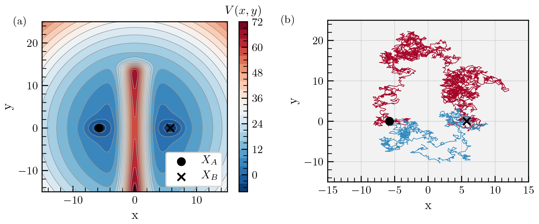
Figure 5(a) Potential landscape of the two-dimensional gradient system defined by Eq. (15). Two energy minima are located at ${\mathit{X}}_A\approx (-\mathrm{5.77},\mathrm{0})$ and ${\mathit{X}}_B\approx (\mathrm{5.77},\mathrm{0})$. They are separated by a potential barrier spanning y<15 and at x=0. (b) Typical transition paths from X_A to X_B for two noise levels σ. At high noise, trajectories can cross the potential barrier (σ=10, blue). At low noise, trajectories go through the upper channel (σ=3, red).

Download

Figure 6a shows a histogram computed with 300 transition paths for the system with the potential given by Eq. (15), with noise level set at σ=3. We need enough trajectories so that the histogram gives an accurate representation of all possible transition paths and that fluctuations along the typical path can be effectively averaged out by the path estimation algorithm. One way to verify that there are enough trajectories is to check that the histogram near the equilibria is similar to the Gaussian stationary distribution that arises from locally linearised Ornstein–Uhlenbeck dynamics. For example, starting from an equilibrium point and picking any direction, then if for the first few histogram cells the histogram value is not decreasing (as would be the case for a Gaussian distribution), this would mean that too few trajectories were used. The typical transition path was estimated using the algorithm sketched in Sect. 2.4. As already mentioned, some artefacts created by the estimation (such as spiraling or zigzagging) can be corrected using a clean-up algorithm. The result is shown in Fig. 6b: the empirical estimation of the typical path resembles the instanton around which the transition paths are clustered at lower noise (Fig. 6b, blue path). The instanton was calculated by implementing the geometric minimum action method (Heymann and Vanden-Eijnden, 2008). Note that if, instead, we accumulated trajectories at high noise σ>10, we would obtain trajectories going from X_A to X_B in a straight line, which is the typical path at high noise similar to Rolland and Simonnet (2015). This typical transition path is then substantially different from the instanton, which goes through the upper channel. Thus, our method can be advantageous in multistable systems where the typical transition path depends on the noise level. We can start at high noise and reapply the empirical estimation of the typical path each time the noise level is decreased.

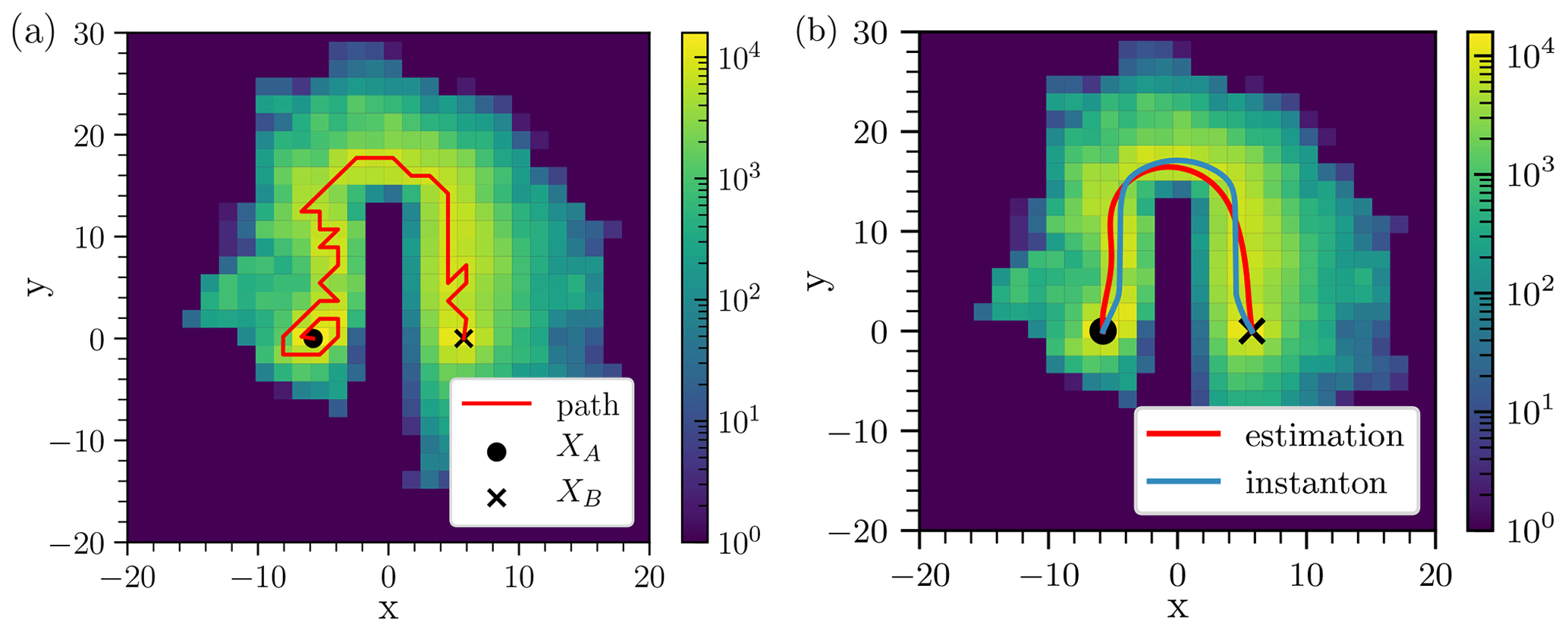
Figure 6(a) Histogram of N=300 transition paths at noise level σ=3, using the modified score function ${\stackrel{\mathrm{̃}}{\mathit{\varphi }}}_{\text{gauss}}$ with β=1.5, defined by Eq. (6) and implemented with Eq. (14). The corresponding transition probability ($p=\mathrm{2}\times {\mathrm{10}}^{-\mathrm{3}}$) is high enough so that direct Monte Carlo sampling could have been used to produce a similar histogram. The bin resolution (Δx=1.4, Δy=1.75) is coarse for illustration purposes. The histogram is used as input in the path-finding algorithm which produces the transition path in red. Grid-scale spiralling occurs near the initial state X_A because of the concentric shell structure of the local probability density function given by Eq. (10). (b) Same histogram as panel (a). The estimated typical transition path (red) has been cleaned up from its grid-scale spiraling and zigzags with the clean-up algorithm and has then been smoothed. It strongly resembles the instanton (blue) which was computed by implementing the geometric action minimum method (Heymann and Vanden-Eijnden, 2008).

Download

Given a typical transition path 𝒞, we present the design of a score function ϕ_𝒞 which encourages trajectories to follow the transition path 𝒞 such that it gives a reasonable approximation of the static committor. Let us consider a trajectory 𝒞(s) in ℝⁿ parameterised by arclength $s\in [\mathrm{0},\mathrm{1}]$. Then we define the score function ϕ_𝒞, called the path-based score function, such that it grows from 0 to 1 along the trajectory from X_A to X_B and decays exponentially along the direction transverse to the trajectory:

where $d(\mathit{X},\mathcal{C})={inf}_{s\in [\mathrm{0},\mathrm{1}]}\Vert \mathit{X}-\mathcal{C}\left(s\right){\Vert }_d$ is the distance between X and the trajectory 𝒞(s), s(X,𝒞) is the curvilinear coordinate of the position on the trajectory that satisfies the infimum in the definition of d(X,𝒞) and d₀ is the characteristic decay length (free parameter). The score function ϕ_𝒞 is shown in Fig. 7 for the estimated transition path 𝒞 shown in Fig. 6 and two values of decay length d₀=20 and d₀=200.

Figure 7(a) Contour levels of the score function ϕ_𝒞 defined in Eq. (16) associated with the estimated transition path 𝒞 shown in Fig. 6 and with decay length d₀=20. (b) Same figure for d₀=200.

Download

The score function increases from 0 to 1 along the trajectory. Thus, it encodes the preferred direction that the system has to follow. This contrasts with the generic score functions ϕ_gauss and ϕ_dist, which are symmetrical in y: they do not contain the information that the system has to increase in y in order to make the transition to X_B. Note that the method we developed here can be applied, in principle, to systems of any dimension. As shown in Fig. 7b, the score function ϕ_𝒞 is discontinuous because the trajectory has positive curvature. The discontinuity is located near the axis x=0. Indeed, when crossing the axis x=0, the closest point on 𝒞 changes and s(X,𝒞) is discontinuous.

Next, we applied TAMS with the path-based score function ϕ_𝒞 to the two-dimensional system in Eq. (15). We compare its performance with the previously defined score functions ϕ_dist and ϕ_gauss. In fact, we use the associated modified score functions, such that the target set B matches the 0.95-confidence ellipsoid (we drop the tildes for readability). We use the following parameters: duration of a trajectory T=20, time step dt=0.01, and N=100 trajectories in the ensemble, which we found was enough to ensure that the interquartile range of the independent realisations spans less than 1 order of magnitude around the mean for most noise levels.

We show in Fig. 8a the transition probability estimates using the score functions ϕ_dist, ϕ_gauss (with β=1.5) and ϕ_𝒞 (with decay parameters $d_{\mathrm{0}}=\mathrm{2},\mathrm{20},\mathrm{200}$) averaged over 10 instances of the algorithm. The probability estimates are in good agreement with each other and with a Monte Carlo estimation for σ>2.5. The score function ϕ_𝒞 is robust with respect to the choice of the decay length d₀.

The performances of the numerical methods are next measured using the work-normalised relative error ϵ, which combines the variance of the algorithm and its computational cost (Glynn et al., 2009):

where ${\mathit{\mu }}_{\widehat{p}}$ and ${\mathit{\sigma }}_{\widehat{p}}$ are the mean and standard deviation of the probability estimate over the different instances, and ω is the average number of time steps calculated in one realisation. In short, ϵ measures how precise the numerical method is at equal computational cost. The smaller the ϵ, the better the algorithm performs.

The results are shown in Fig. 8b. For the system in Eq. (15), the score functions ϕ_dist, ϕ_gauss and ϕ_𝒞 have little difference in performance. For the lowest noise values, the path-based score function has at most a 30 % smaller error ϵ than the score function ϕ_gauss. Changing the decay length d₀ hardly changes the error ϵ. When adjusting the parameters of the potential V or applying the same method to the triple-well system used in Rolland and Simonnet (2015), the performance gain, while often present, never systematically exceeded 30 %. All in all, in this category of two-dimensional systems, using the path-based score function approach yields little improvement.

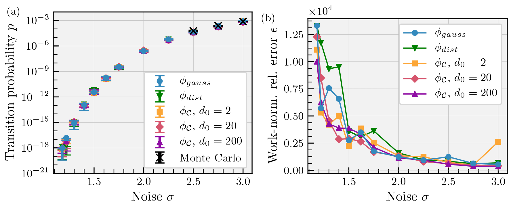
Figure 8(a) Transition probability p as a function of noise parameter σ. Mean estimates and interquartile range (error bars) over N_samples=10 independent realisations of the TAMS algorithm using the score functions ϕ_dist (green down triangle), ϕ_gauss (with β=1.5, blue circle) and ϕ_𝒞 with decay parameters $d_{\mathrm{0}}=\mathrm{2},\mathrm{20},\mathrm{200}$ (yellow square, pink diamond, purple up triangle) are shown. The Monte Carlo estimate (black cross) has been run with $N=\mathrm{5}\times {\mathrm{10}}^{\mathrm{5}}$ trajectories with the target sets coinciding with the confidence ellipsoids around X_B, with associated standard deviation ${\mathit{\sigma }}_p=\sqrt{p(\mathrm{1}-p)/N}$ (error bars). There is an overall good agreement between the numerical estimations. The path-based score function is robust to the choice of decay parameter. (b) Performance of the score functions measured by the work-normalised error ϵ as a function of noise σ (same markers as panel a). At most, there is a 30 % decrease in error when using the path-based score function ϕ_𝒞 at low noise. Note that at high noise σ=3, using a short decay length d₀=2 with ϕ_𝒞 leads to poor performance because the greater values of ϕ_𝒞 are tightly concentrated around the estimated instanton, whereas typical transition paths are not necessarily clustered around it. Otherwise, the performances of the score functions are roughly similar.

Download

3.3 Transition probabilities in a box model of the AMOC

Finally, as a main application of the modification of the target set B into a confidence ellipsoid ℰ, we consider the dynamical system in Castellana et al. (2019), which represents a box model of the AMOC. The system consists of a set of stochastic differential equations, plus one algebraic constraint, the latter representing the salt conservation in the model (as shown in Appendix B). This model can be formulated as

In the equations above, we split the state of the system X_t into two parts: Y_t, which includes salinities of four of the boxes plus the depth of the pycnocline D, and Z_t, which represents the salinity of the deep box (S_d). As the noise is applied only to the asymmetric component of the atmospheric freshwater flux (E_a), it directly affects only two of the variables: S_n and S_s. Moreover, the stochastic increments associated with the two variables are identical to make sure that each decrease in freshwater forcing in the southern box results in the same increase in it in the northern box in the model. Therefore, the noise is not spatially independent, and the noise matrix G is no longer diagonal: it consists of a (5×1) row vector, with only two elements different from zero. For a reasonable choice of the parameters, the deterministic system is in a bistable regime (Castellana et al., 2019), which means that there are two possible equilibrium states under the same forcing conditions. In general, we are interested in studying transitions between the present-day AMOC (X_A) and the collapsed state (X_B).

For a differential-algebraic system of equations (DAEs), such as the system in Eq. (18), we need to be particularly careful while computing the covariance ellipsoids. First of all, we make use of the Schur complement of the Jacobian of the system, which allows us to calculate the covariance matrix when an algebraic constraint is present (Baars et al., 2017). Nevertheless, the resulting matrix C_B is singular, with two eigenvalues being equal to zero. One of the corresponding eigenvectors is a vector pointing in the direction of the variable D (depth of the pycnocline). The reason behind it is that the differential equation governing the evolution of D does not contain any of the other variables (see Castellana et al., 2019) when the system is in the collapsed state (X_B). This results in D not being affected by the noise, as this is imposed only on two of the salinities. Hence, we compute the covariance matrix ${\mathbf{C}}_B^S$ relative to the salinities, removing 1 degree of freedom from the original matrix. Unfortunately, such a matrix still has one zero eigenvalue, which is due to the salinity conservation (the algebraic equation in the system Eq. 18). To overcome this problem, we compute the Moore–Penrose inverse (or pseudo-inverse) of the covariance matrix, ${\mathbf{C}}_B^{S+}$, by performing a singular value decomposition of ${\mathbf{C}}_B^S$ and removing the zero eigenvalue, together with the corresponding eigenvector (Ben-Israel and Greville, 2003). A two-dimensional projection of the ellipsoid constructed for the box model is shown in Fig. 9.

For the system in Eq. (18), the modified score function is more complicated, as the covariance matrix used to construct the ellipsoid contains only the degrees of freedom related to the salinities of the model, leaving the variable D (depth of the pycnocline) out. From a geometric point of view, that means that the covariance ellipsoid around X_B is degenerated along the D direction. Figure 9 shows a projection of the ellipsoid – once the noise amplitude is fixed – onto the plane identified by the variables S_n and S_s (respectively, the salinity of the northern box and the one of the southern box in the model). The projection was obtained by calculating the conditional covariance matrix of the two variables under consideration, given that the other variables are set on their mean value (Wasserman, 2013). The two-dimensional ellipse contains the large majority of the projected time points (on the same plane) of a trajectory that wanders around the equilibrium. By construction, the confidence level of the confinement is higher than the one prescribed for the full-dimensional ellipsoid (in this case 0.95). Clearly the level sets of the score function ϕ_gauss do not coincide with the one of the ellipsoid. Hence, the importance of modifying the score function appears evident.

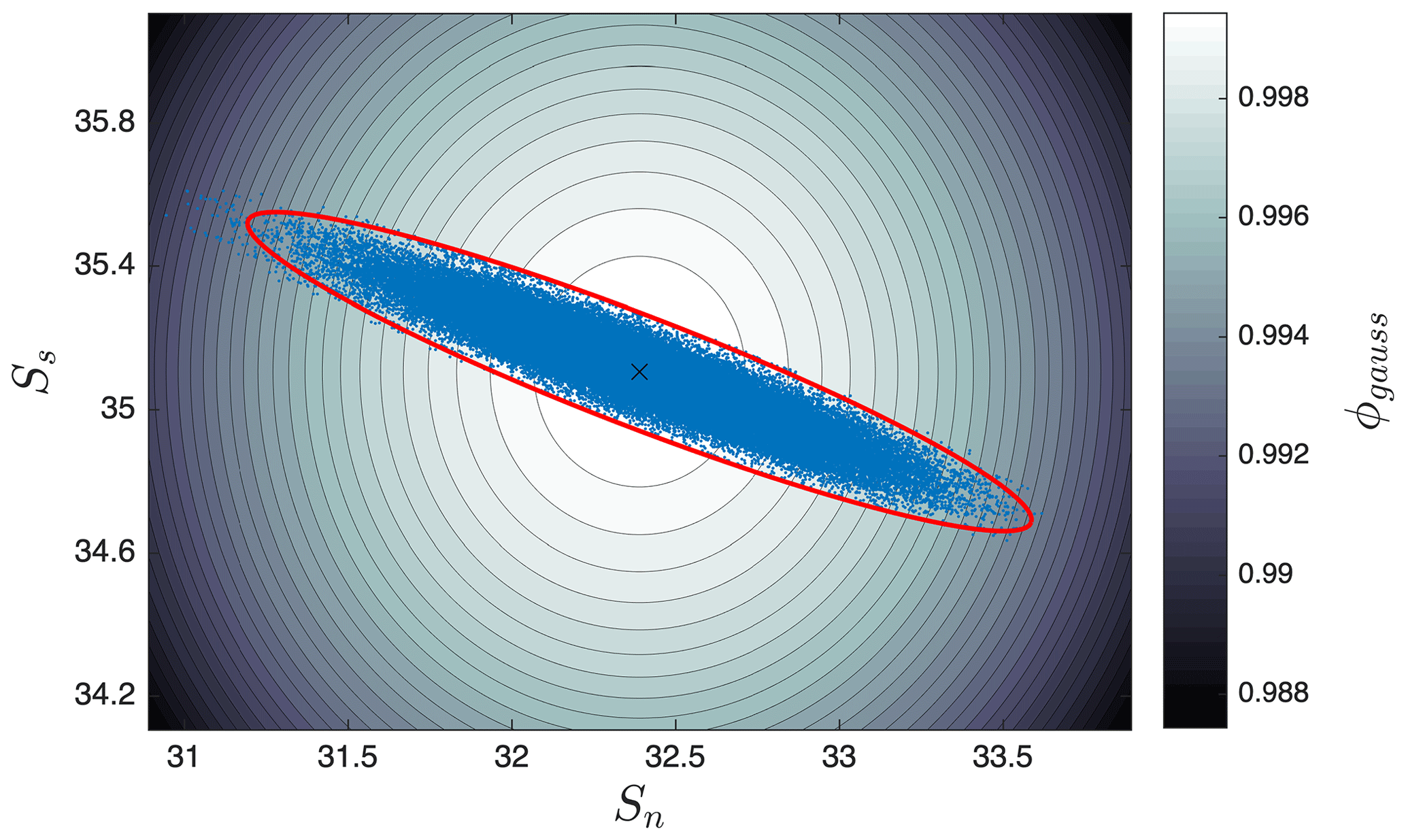
Figure 9Level sets of the score function ϕ_gauss in proximity to the collapsed equilibrium state X_B of the system in Castellana et al. (2019), projected onto the plane identified by the variables S_n and S_s (respectively, the salinity of the northern box and the one of the southern box in the model). A trajectory of the system, initiated in the collapsed state, has been projected onto the same plane (blue circles). The red ellipse is the two-dimensional projection of the covariance ellipsoid constructed by using the matrix ${\mathbf{C}}_B^S$ and a confidence level of 0.95; 98 % of the points comprising the trajectory are inside the ellipsoid.

Download

When constructing an improved score function, in order to evaluate whether a state belongs to the neighbourhood of X_B, we need to check two conditions: (i) whether the state of the system is inside the salinity covariance ellipsoid drawn around the destination equilibrium and (ii) whether the variable D of the state is the same as the one of X_B. Hence, the improved score function for the box model reads as

where X^S indicates the part of the state vector representing the set of the salinities, whereas X^D represents the variable D. As already mentioned, to check whether a certain state belongs to the salinity ellipsoid, we made use of the pseudo-inverse of ${\mathbf{C}}_B^S$ in the definition of Eq. (12).

To be able to assess the relevance of a proper definition of the target set in the TAMS algorithm and hence the importance of using the improved version of the score function, we computed transition probabilities of the AMOC from the present-climate state to the collapsed state for reasonable values of the atmospheric forcing and noise. In particular, we chose ${\overline{E}}_{\mathrm{a}}=\mathrm{0.20}\mathrm{Sv}$ and f_σ=0.16. This last value represents the ratio between the standard deviation of the noise in the atmospheric forcing and its mean value (Castellana et al., 2019). The number of trajectories used in the algorithm was set to 100, and the timescales at which the probabilities were evaluated were chosen to be 1000 and 10 000 years, respectively. For each transition probability, we used three different versions of the algorithm, based on three different settings for the score function. The first two versions were implemented by using ϕ_gauss in Eq. (6), with two different choices for the threshold ϕ^target. In the third version, we used ${\stackrel{\mathrm{̃}}{\mathit{\varphi }}}_{\text{box}}$ as defined in Eq. (19), where the starting score function was ϕ_gauss. Each probability was calculated by running 15 instances of the algorithm and then computing the median and the interquartile range (IQR). The results are shown in Table 1 below.

Table 1Results of the transition probabilities for the AMOC model using different score functions.

Download Print Version | Download XLSX

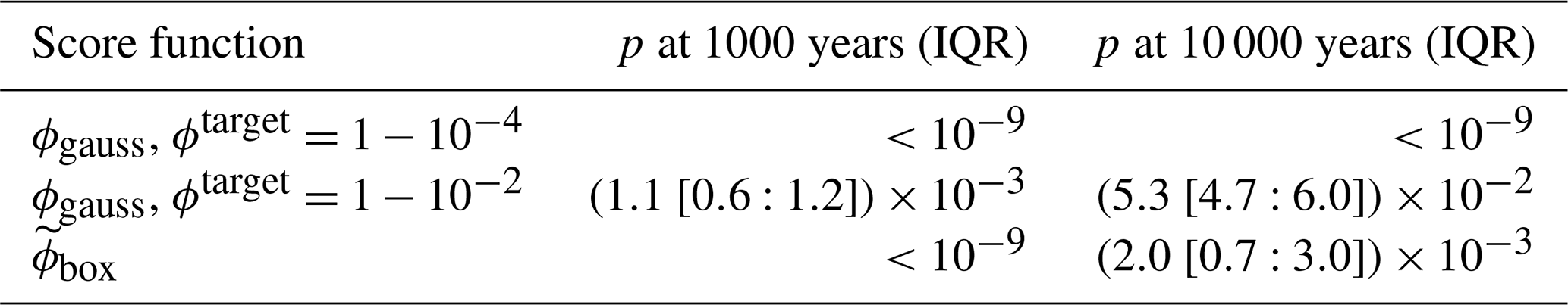
When running TAMS to compute transition probabilities between two states of the Atlantic circulation in this model, with different versions of the score function, we found a considerable discrepancy between the obtained values. In particular, it appears that setting a very high threshold in the Gaussian score function makes the algorithm detect no transitions (we set up the algorithm so that it stops when the probabilities involved are smaller than 10⁻⁹): the reason behind this is that, because of the presence of the noise, we do not expect the state of the system to stay indefinitely close to the destination equilibrium but rather to wander around it. Therefore, the score function, which assigns the maximum score only to a very small neighbourhood of the equilibrium, is not able to properly recognise transitions. Moreover, it is not surprising that, when using ϕ_gauss with a smaller value of ϕ^target (0.99) or ${\stackrel{\mathrm{̃}}{\mathit{\varphi }}}_{\text{box}}$, we obtain different results: as the shape of the covariance ellipsoid is not spherical (see Fig. 9), we expect ϕ_gauss to detect transitions even though the state is actually still far from the destination equilibrium, at least in certain directions. As a general rule, we expect ϕ_gauss to give results different from ϕ_box as long as the ellipsoid of the system is not spherical, regardless of the choice of the threshold ϕ^target.