
Landsat and Sentinel-2 Based Burned Area Mapping Tools in Google Earth Engine


1
Department of Mining and Metallurgical Engineering and Materials Science, School of Engineering of Vitoria-Gasteiz, University of the Basque Country UPV/EHU, Nieves Cano 12, 01006 Vitoria-Gasteiz, Spain
2
Environmental Remote Sensing Research Group, Department of Geology, Geography and the Environment, Universidad de Alcalá, C/Colegios 2, 28801 Alcalá de Henares, Spain
*
Author to whom correspondence should be addressed.
Remote Sens. 2021, 13(4), 816; https://doi.org/10.3390/rs13040816
Submission received: 9 December 2020
/
Revised: 18 February 2021
/
Accepted: 19 February 2021
/
Published: 23 February 2021
(This article belongs to the Special Issue Remote Sensing of Burnt Area)
Abstract
:Four burned area tools were implemented in Google Earth Engine (GEE), to obtain regular processes related to burned area (BA) mapping, using medium spatial resolution sensors (Landsat and Sentinel-2). The four tools are (i) the BA Cartography tool for supervised burned area over the user-selected extent and period, (ii) two tools implementing a BA stratified random sampling to select the scenes and dates for validation, and (iii) the BA Reference Perimeter tool to obtain highly accurate BA maps that focus on validating coarser BA products. Burned Area Mapping Tools (BAMTs) go beyond the previously implemented Burned Area Mapping Software (BAMS) because of GEE parallel processing capabilities and preloaded geospatial datasets. BAMT also allows temporal image composites to be exploited in order to obtain BA maps over a larger extent and longer temporal periods. The tools consist of four scripts executable from the GEE Code Editor. The tools’ performance was discussed in two case studies: in the 2019/2020 fire season in Southeast Australia, where the BA cartography detected more than 50,000 km2, using Landsat data with commission and omission errors below 12% when compared to Sentinel-2 imagery; and in the 2018 summer wildfires in Canada, where it was found that around 16,000 km2 had burned.
Keywords:
burned area; Australia; Canada; tools; validation; Landsat; Sentinel-2; Google Earth Engine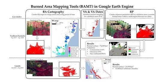
1. Introduction
Biomass burning is a significant disturbance that causes soil erosion and land-cover changes and releases greenhouse gas emissions into the atmosphere, also affecting people’s lives and properties [1,2,3]. Fires are present in most types of vegetation in the world, especially grasslands, savannas, and forest, and they occur on all continents, with a significant incidence in Africa, which accounts for 70% of the global burned area [4,5,6]. Therefore, burned areas (BAs) must be detected accurately both spatially and temporally, for which satellite Earth observation has been much used over the last few decades, especially using coarse spatial resolution [5,6,7,8,9,10,11,12,13,14]. Global products at coarse spatial resolutions have significant omission errors [4,15,16,17,18], but creating products at medium resolution, although more accurate, is also quite challenging: It implies a heavy data-processing workload, and the temporal resolution is low (typically one image every 5 to 16 days).
Using BA mapping with medium spatial resolution had been operationally quite limited until Landsat historic imagery became freely available in 2008, since the scientific literature on this topic had been mainly limited to single or neighboring scenes [19,20,21]. In addition, since 2015, the Sentinel-2 imagery has added a large volume of imagery that makes it possible to analyze time series at a medium spatial resolution. A few BA automatic algorithms have been developed, using time series data, especially using Landsat data [22,23,24,25], albeit also using Sentinel-2 [16,26], or a combination of the two [27]. So far, the only example of a global product based on medium-resolution data is Global Annual Burned Area Map (GABAM) [23], obtained for 2015, using Landsat data. At the continental level, it is worth mentioning the Landsat Burned Area Essential Climate Variable (BAECV) covering the Conterminous United States (CONUS) [25,28], the province of Queensland in Australia for the whole Landsat historical database [29] and the sub-Saharan Africa in 2016 [16].
Despite this effort to develop automatic algorithms, supervised multitemporal image analysis is considered to be a superior method for the purpose of mapping burned areas. In fact, it allows for differentiation between old and new burns, and reliably detects small spatially fragmented low-combustion completeness burns. It also enables gross errors that may occur in satellite data to be accommodated, and differentiates between burned and spectrally similar unburned features [30]. For example, supervised analysis of higher spatial resolution imagery is adopted as the validation protocol for BA mapping [31]. Although visual interpretation and delineation are generally recommended [12,30,32,33], these processes usually take the form of a supervised semi-automatic classification that is visually checked and manually refined [15,34]. Compared to the field-based classical methods used to report official statistics on burned areas, remote sensing-based mapping is more objective and efficient, less labor- and time-consuming and more repeatable [35].
In 2014, the University of the Basque Country (UPV/EHU) developed a software for supervised BA mapping, using Landsat data: Burned Area Mapping Software (BAMS). This software was basically designed to process a pair of Landsat images at a time, allowing for BA mapping between the two scenes, using a two-phase mapping strategy, thus obtaining the burned polygons in a vector layer [36]. It provided good cost efficiency, although it relied on the processing capacity of the user’s computer and was based on a commercial GIS software. The software was widely used to create validation areas inside the Fire_cci project [15,37,38], as well as for the USGS Burned Product initial validation, and many other fire science-related users, environmental techniques and the commercial community [16,28,37,39,40,41]. However, several limitations were also detected and discussed with users. Firstly, it was only applicable to Landsat data and was unable to process Sentinel-2 data. Secondly, the software was not easily maintained as metadata and the Landsat data format changed and its proper functioning was interrupted several times. Finally, the BAMS mapping methodology trained only the burned category and saved time for the user, but the user was unable to control the unburned category properly; thus, a manual edition was often necessary to remove commission errors in agricultural areas and cloud shadows.
Google Earth Engine (GEE) is a free cloud-computing platform for satellite data processing, with several data catalogs at different resolutions (notably Landsat, Sentinel-2 and MODIS) and planetary-scale analysis capabilities (https://earthengine.google.com (accessed on 27 January 2021)) [42]. Since the first significant work on the topic was published in 2013 [43], the number of studies using GEE has dramatically increased, with more than 200 papers having been published in 2019 [44], covering all types of applications, such as vegetation mapping and monitoring, land-cover mapping, agricultural applications, and disaster management and Earth sciences [45]. However, there have not been so many published papers on the fire field [23,46,47,48].
This study presents several tools that we have developed and released in GEE. These tools are referred to as Burned Area Mapping Tools (BAMTs), and they cover the entire BA mapping process: from creating a large extent BA map to creating statistically design samples for validation studies and the actual generation of BA reference perimeters (RPs), using both Landsat and Sentinel-2 images. The study describes these tools and provides two case studies that were applied in the Australian fire season between 2019 and 2020, and in the Canadian wildfires from the summer of 2018. All four tools and the user guide are totally free and can be reached at https://github.com/ekhiroteta/BAMT (accessed on 27 January 2021).
2. BAMT Tools
Four tools have been developed for BA mapping:
- BA Cartography: The user can create a BA product over a large region and a long period of time, from changes between two temporal images via a supervised classification.
- VA: for validation area (VA) selection based on several strata, in accordance with an existing stratified random sampling methodology.
- VA Dates: This tool serves as a bridge between VA and RP tools, providing the user with information about which dates to use to generate RP, after having sampled the best validation areas, i.e., identifying cloud-free dates.
- RP: creates accurate burned areas within a small region, from changes between two dates via a supervised classification. It is mostly oriented towards generating reference perimeters (RPs) for a BA product’s assessment.
2.1. Datasets and Preprocessing
BAMT rely on the Landsat and Sentinel-2 datasets that are uploaded to the GEE environment. The Landsat program is a NASA/USGS program for satellite imagery acquisition and Earth observation [49], with a series of satellites that started acquiring images in 1972 with Landsat-1, being the last satellite launched in 2013, and over 8 million scenes of the Earth having been acquired since then. From its seven satellites, only Landsat-4 and -5 Thematic Mapper (TM), Landsat-7 Enhanced Thematic Mapper Plus (ETM +) and Landsat-8 Operational Land Imager (OLI) data are used in BAMT. They provide continuous global coverage since 1982, acquiring images every 16 days (reduced to 8 days in years where two satellites are operational) at 30 m of spatial resolution and covering the visible, near infrared (NIR) and short wavelength infrared (SWIR) spectral regions. From all available Landsat products in GEE, the Landsat Tier 1 Surface Reflectance (SR) [50,51] product was the one selected, which includes atmospherically corrected and orthorectified surface reflectance data for four visible and near-infrared (VNIR) and two short wavelength infrared (SWIR) bands. These products are represented by the following IDs in GEE: ‘LANDSAT/LT04/C01/T1_SR’ for Landsat-4 TM, ‘LANDSAT/LT05/C01/T1_SR’ for Landsat-5 TM, ‘LANDSAT/LE07/C01/T1_SR’ for Landsat-7 ETM + and ‘LANDSAT/LC08/C01/T1_SR’ for Landsat-8 OLI.
The European Space Agency (ESA) developed the Sentinel-2 mission (S2) as part of the EU Copernicus program [52], with two satellites working simultaneously (Sentinel-2A and Sentinel-2B) since 2017. Both incorporate the Multi-Spectral Instrument (MSI), an optical sensor similar to those aboard the Landsat satellites, albeit with improvements in spectral, spatial and temporal resolutions. MSI covers the globe at 10 or 20 m, depending on the spectral band, with a revisit time of 10 days (from June 2015 onwards, when Sentinel-2 A was launched) and 5 days (from March 2017, after the launch of Sentinel-2B) by combining both satellites, obtaining 2–3 days of revisit time in mid-latitudes, due to the overlap between adjacent orbits. Two Sentinel-2 products are available in GEE: Level-1C (L1C) and Level-2A (L2A), with the corresponding ‘COPERNICUS/S2S and ‘COPERNICUS/S2_SR’ dataset IDs. The bands in the former product contain Top of Atmosphere (TOA) reflectance, although the latter has Bottom of Atmosphere (BOA) reflectance and a scene classification (SCL) including quality indicators such as cloud probabilities and snow [53].
Although BAMT could use L1C and L2A products, there are critical differences between them that make the first-mentioned product preferable. On the one hand, the topographic correction applied in L2A creation [54] gives rise to an overcorrection of mountain shadows and an artificial effect in mountainous regions, even though this does not occur in every image (Figure 1). On the other hand, the L2A product is not globally produced for the completely temporal coverage of Sentinel-2; although 2019 and 2020 have the same number of scenes for both products in GEE, 2015 and 2016 do not have any L2A scenes, and there are only a few for 2017 and 2018 (Figure 2).
Six reflectance bands common to all four sensors (TM, ETM +, OLI and MSI) are employed: the three visible colors (blue, green and red), the near infrared (NIR) and two short wavelength infrareds (short and long SWIRs). Each of these bands’ wavelengths may vary among different sensors, but they cover an equivalent region in the spectrum (Table 1). Landsat bands are available at 30 m spatial resolution. S2 MSI visible bands are at 10 m and both SWIRs at 20 m; there are two NIR bands, each at a different resolution, as indicated in Table 1.
The Quality Assessment (QA) band for both sensors has been used to identify pixels that exhibit adverse instrument, atmospheric or superficial conditions (Table 2). The pixel_qa band for Landsat images indicates the presence of cloud shadows and clouds in the 3rd and 5th bits, respectively, while the QA60 band of S2 data contains similar information in its 10th and 11th bits, even though this does not indicate the presence of cloud shadows. In the RP tool, the SCL is used instead of the QA60 quality band if a L2A scene is available since it is more accurate; this SCL includes several cloud probabilities and a cloud shadow category that are crucial for masking purposes. In addition, an empirical threshold based on the B1 band has been employed to avoid the heavily underestimated presence of clouds of the Level-1C product [55]: B1 higher than 1500, or a more relaxed threshold of 2000 if SCL from L2A is used. In our developmental experiments, this band, at 60 m of spatial resolution, has shown the best performance of BA mapping in cloudy areas.
The normalized difference between the most important spectral spaces for the BA was added to the selected spectral bands described in Table 1, as follows: Normalized Difference Vegetation Index (NDVI) [56] in the red/NIR space, Normalized Burned Ratio (NBR) [57] in the NIR/Long SWIR and Normalized Burned Ratio 2 (NBR2) [19] in the Long SWIR/Short SWIR space. The equations for these indices are as follows:
where ρRed = reflectance in the red band, ρNIR = reflectance in the NIR band, ρShortSWIR = reflectance in the Short SWIR band, and ρLongSWIR = reflectance in the Long SWIR band.
NDVI = (ρNIR − ρRed)/(ρNIR + ρRed)
NBR = (ρNIR − ρLongSWIR)/(ρNIR + ρLongSWIR)
NBR2 = (ρShortSWIR − ρLongSWIR)/(ρShortSWIR + ρLongSWIR)
2.2. BA Cartography Tool
The purpose of this tool is to generate a BA vector map in a user-defined area and period via a supervised classification of Landsat or Sentinel-2 data, as defined by the ‘dataset’ parameter. The flowchart of the tool below illustrates its logic (Figure 3).
The processing area extent has to be manually digitized in the ‘studyArea’ predefined geometry layer of the script and could be a region, country or even a continent (the process might lead to an error if the processing area is too large, because the user memory could be exceeded). Two consecutive periods must be defined (by ‘date_1′, ‘date_2a and ‘date_3a parameters), namely the pre- and post-fire periods, with the second one beginning the day following the end of the first period. The individual imagery involved in the region, dataset and period defined are masked using the rules described in Table 2 and the NDVI, NBR and NBR2 spectral indices are computed for each scene. Pixel-based temporal composites are computed for both post-fire and pre-fire periods (Figure 4a,b), taking the one with the minimum NBR from the dates available. In our experiments, this band evidenced the best compositing performance, by maximizing or minimizing the individual bands and spectral indices, and retaining the dates’ pixel value when the burned signal was considered strongest. Temporal compositing has many advantages in processing frameworks, especially if the analysis covers large areas [58]. Post-fire and pre-fire composites are used to compute the composite subtraction (Figure 4c), and thus another nine bands are obtained over the user-defined extent, six reflectance bands and three spectral indices.
A Random Forest (RF) classifier is trained, using the burned and unburned samples the user digitized in the ‘burned’ and ‘unburned’ layers within the GEE Code Editor environment. These samples are digitized over a Long SWIR/NIR/red color composition of the pre-fire composite, post-fire composite and pre-fire/post-fire difference visualized over the GEE map. Among other data-mining algorithms included in GEE, such as Classification and Regression Tree (CART) [59], Naive Bayes and Support Vector Machine (SVM) [60], RF was selected because of the fast training and prediction involved, unconstrained by the distribution of the predictor variables, reduced overfitting, robustness to outliers and non-linear data. RF classification also handles unbalanced data that are common in BA mapping. Indeed, this technique has become popular within the remote sensing community due to the accuracy of its classifications [61]. A Random Forest classifier is an ensemble classifier that produces multiple decision trees, using a randomly selected subset of training samples and variables [62]. GEE implementation default parameters were maintained for all parameters (the square root of the number of variables as the number of variables, a 0.5 fraction of input to bag per tree, unlimited maximum nodes), except for the number of trees (500), as recommended in a study [61], and the minimum number of elements in each node (10). Each time the user redefines burned and unburned samples and executes the script, a probability image is obtained, with values ranging from 0% (unburned) to 100% (burned) (Figure 4d).
The algorithm ends by applying a two-phased strategy on the output probability image of the RF model in order to map the burned areas, an efficient strategy to balance omission and commission errors [36,63]. Patches of pixels with a probability higher than 50% using a 4-node connection (the only group of pixels that share an edge) are labeled as burned, as long as they contain at least one seed pixel inside. These burned seeds are pixels with higher probability than the average of the mean RF probabilities obtained for the training polygons (Figure 4e). When the algorithm is executed and the results visualized, the user may modify or define more training polygons and re-run the algorithm repeatedly, until the desired visual accuracy is obtained. The end result (only burned or unobserved areas, but not observed and unburned areas) can be exported in ESRI (Environmental Systems Research Institute) Shapefile format in a 2 × 2-degree grid to the user’s Google Drive account (Figure 4f). The grid was fixed to 2-degree tiles because larger tiles were likely to exceed GEE user memory limit, although if the limit is still exceeded, the 2-degree tile can be split into smaller tiles (see user guide). The polygon vector layer assigns the fire detection date from the post-fire composite, computing the mode (most repeated date) for each burned patch.
2.3. VA Tool
The Committee on Earth Observing Satellites (CEOS) Working Group on Calibration and Validation (WGCV) first defined validation as ‘the process of assessing by independent means the quality of data products derived from the system outputs’ [64]. Satellite product performance information is required to enable users to select and use products appropriately [65,66]. The independent reference data’s characteristics influence the reliability and the degree to which validation results are representative of the validated product [33], while the validation sampling design is critical in making the most out of the reference data. Probability sampling designs ensure that accuracy inferences are possible on a global scale [21].
The first inferences of global product accuracies became available a few years ago [15,34]. A great deal of attention was placed on (1) defining the sampling units by attributing them with spatial and temporal dimensions so that accuracy inferences could be made for specific spatial and temporal extents [33], and (2) improving the efficiency of sampling designs to obtain accuracy inferences as precise as possible given a sample size [67]. These methodologies were based on Landsat data, which most global BA validation exercises used. Firstly, two sampling grids were created: a spatial grid, based on Thiessen Scene Areas (TSAs) [68,69], and a temporal grid, consisting of two consecutive image acquisition dates. Two levels of stratification were then applied on the spatial and temporal sampling units: the predominant Olson biome [70], first reduced to seven main categories [33,34], and the fire activity in each sampling unit. Depending on the study, either the BA extent provided by the Global Fire Emissions Database version 3 (GFED3) [71] or the number of hotspots in the MODIS active fire product [72,73] was used as a reference for fire activity, delimited spatially by the extent of the TSA and temporally by its acquisition dates. Sampling units in each biome were split between low and high fire activity strata, resulting in 14 strata in total. Finally, the number of sample sizes for each stratum was computed proportionally to the number of sampling units in the stratum. However, this method assumed that all Landsat acquisitions were available and that the clouds did not affect them, while the ground’s observability was not actually secured, as mentioned by Boschetti et al. [33]. In addition, the short temporal length of sampling units (16 days between two consecutive Landsat images) may increase the validated BA product’s estimated errors if burning dates are not identified accurately in the global product. To solve these issues, ‘long sampling units’ have been employed in recent studies [6,14,16]. These units are typically over 100 days long, with a minimum frequency of an available image every 16 days, whereas previous 16-days-long units are referred to as ‘short sampling units’.
The VA tool used in this study is an adaptation of this stratified random sampling methodology, not only for sampling validation areas for coarse resolution BA products, but also for the BA maps obtained using medium spatial resolution with the BA Cartography tool in BAMT. Several decisions were taken to adapt the algorithm to this tool:
- Sentinel-2 data were incorporated into the analysis, as these offer better spatial and temporal resolutions than Landsat data and should improve reference data created for the BA validation. The user may thus choose between S2 or Landsat data (with the ‘dataset’ parameter).
- Landsat or S2 scene extents are considered as sampling units instead of TSAs. Despite using whole TSAs when applying the stratified random sampling methodology, most studies have only created reference data in a central window of about 20–30 km wide and high [6,14,16,37], which the fire activity cover value used in the analysis might not properly represent. Therefore, the user can define the dimension of a square window (‘dimension’ parameter), located at the center of the scene, so that the analysis may be carried out in that specific window.
- Either the MCD64A1 [5] or the FireCCI51 [6] can be used to estimate global fire activity to select the samples (‘globalBA’ parameter). Both products are available in GEE. The latter has a higher spatial resolution (250 m), but was only processed between January 2001 and December 2019, while the MCD64A1 at 500 m has been systematically processed from November 2000 up to the present.
- Optionally, several criteria of data availability are considered when creating long sampling units: minimum length of the unit in days, minimum frequency of available images in days and maximum cloud cover in each available image (‘minLength’, ‘minFreq’ and ‘maxCloud’ parameters, respectively).
The tool samples a number of validation areas (‘numberVA’ parameter) over a period defined by two dates (‘date_pre’ and ‘date_post’) and spatially delimited by a polygon that is manually defined in the ‘studyArea‘ layer. Firstly, it selects the predominant Olson biome and computes the burned surface (according to the BA product, MCD64A1 or FireCCI51) in each sampling unit. Then, it splits the units into 14 strata, consisting of 7 Olson biomes and two low/high BA strata. The validation areas are then sampled from each stratum proportionally to the number of sampling units in it.
If the optional criteria of data availability are applied, long sampling units that do not fulfil these criteria are removed, and the stratified random sampling is then applied to the remaining units. This assures a long data series with frequent cloud-free data from which high-quality reference data will be created.
2.4. VA Dates Tool
The validation areas sampled by the VA tool do not propose the specific images to be used for reference data creation, and only the scene is identified. Since the CEOS Land Product Validation team recommends that reference fire perimeters be obtained from multitemporal pairs of images in order to properly date the validation period, this tool identifies the images available in the specified scene and period. The identified images also meet a cloud cover criterion the user defines to ensure only cloud-free images are shown.
2.5. RP Tool
Validation of remote-sensing-derived products requires independent reference data and must be obtained with minimum error, either by visual interpretation [12,30,32] or by applying a semi-automatic algorithm followed by visual checking and manual refinement [15,34,74]. Coarse spatial resolution BA products have been validated in accordance with the protocol endorsed by the Committee on Earth Observation Satellites (CEOSs), which is based on product comparison with BA maps interpreted from higher spatial resolution satellite multi-date image pairs [32]. Validating medium spatial resolution BA products is more challenging because interpreting multi-date higher spatial resolution data with a temporal resolution high enough to capture the rapidly evolving burning is expensive and often unavailable, and requires a large and representative independent reference dataset collected via a suitable spatiotemporal sampling, in order to obtain statistically rigorous accuracy measures [27].
This tool focuses on easing the BA mapping process between two single Landsat or Sentinel-2 scenes with the highest possible accuracy, so they can then be used as reference perimeters (RPs) for lower spatial resolution BA assessment purposes, in accordance with the CEOS’s BA assessment protocol. The BA mapping process is similar to the BA Cartography tool in that it digitizes ‘burned’ and ‘unburned’ samples, a RF model with the same parameters is trained, and the user may redefine the training samples until the result is accurate enough, which is then exported in an ESRI Shapefile to the user’s Google Drive account. A label is attached for each polygon, indicating whether it was burned or unobserved accordingly. However, there are some significant differences compared to the BA Cartography tool:
- Spatially, BA detection is limited to a window located at the center of a Landsat or Sentinel-2 scene. The user defines the width and height of the window (‘region_dimension’ parameter).
- Temporally, two single scenes are used for BA detection instead of temporal composites, defined by two dates. The VA Dates tool can be used to identify the dates with available images.
- For Sentinel-2 derived RP, the SCL image is selected to mask clouds and cloud shadows due to its higher accuracy, if an L2A scene is available on the corresponding date; if there is no L2A scene, QA60 and B1 bands are used. L1C TOA reflectance is used to map BA in both cases.
- A more permissive probability threshold defines the burned seeds because the region of interest is smaller and both burned and unburned areas have greater homogeneity across the image. Instead of the average of mean probabilities used in the BA Cartography tool, the minimum among mean probabilities in each burned training polygon is used as the threshold.
- RP from Landsat data are obtained at 30 m, but Sentinel-2 based RP can be obtained at both 20 and 10 m (depending on the ‘resolution’ parameter). If a 10 m output resolution is selected, the B8 band is used instead of B8A (at 20 m) in the NIR region, and this is joined to the visible bands at 10 m (blue, red and green) and both SWIR bands at 20 m. If the 20 m output resolution is selected, the B8A is used as the NIR band. Figure 5 shows how bands at different resolution can be combined, where the NBR index at 10 m is significantly more accurate than the same index at 20 m, despite both indices deriving from the same SWIR band at 20 m.
2.6. Case Studies in Southeast Australia and Canada
We selected two case studies to demonstrate BAMT’s applicability for BA mapping at medium spatial resolution data. In the Southeast Australia (SEA) fire season between 2019 and 2020, the set of four BAMT described in this paper were applied by employing Landsat data to map BA and Sentinel-2 for validation purposes. The second case study employed only the BA Cartography tool to map Canada’s burned areas in the summer of 2018, using Sentinel-2 data, and the areas were then compared to the Canadian National Fire Database fire polygon data available from the Canadian Wildland Fire Information System (CWFIS).
2.6.1. Southeast Australia
The area selected in the SEA case study comprises four different states and territories, covering an area of 1.05 M km2: New South Wales (NSW), Victoria (VIC), Australian Capital Territory (ACT) and Jervis Bay Territory (JBT) (Figure 6a). In this area, the selected 2019/2020 fire season was unusually severe, as bushfires were consequently exacerbated by extreme weather conditions and further caused several social impacts [75,76,77]. A BA product detected between the 1 September 2019 and 30 April 2020 was created, using the BA Cartography tool, employing 2-month-long Landsat composites, both for post- and pre-fire conditions. Therefore, the fire season was divided into 4 bimonthly periods (1 September to 31 October, 1 November to 31 December, 1 January to 29 February, and 1 March to 30 April). Although most fires in SEA were extinguished by the end of February 2020, some were not detected until March 2020 as a result of the gaps caused by clouds in Landsat images. For each post-fire composite, the previous bimonthly composite was used as the pre-fire condition, e.g., the BAs from January to February 2020 were detected by comparing their composite with the November–December 2019 period.
The VA tool sampled 10 validation sites, consisting of 50 × 50 km2 windows located at the center of the S2 tiles. The sites were sampled by applying the optional criteria of data availability, and thus a minimum length of 100 days, a minimum frequency of 20 days between consecutive images and a maximum cloud cover of 30% were required for each long sampling unit. This way, the sampled validation sites were guaranteed to contain frequently available cloud-free S2 images. The MCD64A1 BA product was used as a reference for fire activity. Reference perimeters for each pair of consecutive images in these validation sites were created at 20 m, using the RP tool, in 50 × 50 km2 squares at the center of the S2 tiles. Any pixel that was not observed in any single image was labeled as unobserved for the entire validation period, and only pixels observed through the whole period remained. Among the observed pixels, burned areas were made up of pixels burned in any pair of images. For their part, the accuracy metrics were based on the error matrix approach [78] between the Landsat BA map and the reference perimeters. The commission and omission errors (CEs and OEs, respectively) and the Dice coefficient (DC) were computed for each validation area and also globally. The DC is defined as the probability that one classifier (product or reference data) may identify a pixel as burned, given that the other classifier also identifies it as burned [15,79,80].
The BA product’s temporal accuracy was assessed by comparing product detection dates and VIIRS (Visible Infrared Imaging Radiometer Suite) active fire dates [81]; these hotspots were derived at 375 m from the Visible Infrared Imaging Radiometer Suite sensor aboard the Suomi-NPP satellite. For each VIIRS hotspot, the burned pixel temporally closest to the hotspot was chosen within a 375 × 375 m2 window around the active fire (the active fire product’s spatial accuracy). This closest burned pixel was considered to be part of the burned area whose fire was detected, and its date was compared with that of the hotspot.
2.6.2. Canada
The second case study is located in the 10 provinces of Canada: British Columbia (BC), Alberta (AB), Saskatchewan (SK), Manitoba (MB), Ontario (ON), Québec (QC), Newfoundland and Labrador (NL), Prince Edward Island (PE), Nova Scotia (NS) and New Brunswick (NB) (Figure 6b). This covers the whole of Canada, except for the three territories (Yukon, Northwest Territories and Nunavut), amounting to a total of 6.06 M km2. The 2018 fire season was quite severe, especially in BC, which experienced its worst fire season on record [82] with more than 2000 fires and 1.35 million hectares burned [83,84]. Fires mostly occurred between May and August [85]. Since a 4-month period could be quite difficult to handle in such a large study area, only fires from July and August were detected in this case. However, since some fires from August were not observed in S2 data until September, the period was extended to include this third month.
The BA product was obtained from Sentinel-2 MSI data at 20 m, using the BA Cartography tool. Reference perimeters were not created by using BAMT tools in this case study, but instead were downloaded from the website of the Canadian Wildland Fire Information System (CWFIS) (https://cwfis.cfs.nrcan.gc.ca/datamart (accessed on 27 January 2021)). These perimeters consisted of polygons with an associated burning date. Since the perimeter accuracy varied among provinces as a result of the different mapping techniques [86,87] and some were observed as having coarser spatial resolution than the BA product, only a visual comparison was made, and commission and omission errors were not computed. The BA map’s temporal accuracy was assessed in the same way as in SEA, by comparing burned area dates and VIIRS hotspots.
3. Results
3.1. Southeast Australia
3.1.1. BA Cartography
The BA map for the 2019/2020 fire season in SEA was generated, using the BA Cartography tool, divided into four independent periods. Table 3 shows the number of burned and unburned training polygons digitized in each period, and the number of times (iterations) the script was executed until a visually satisfactory result was obtained throughout the study area. A larger number of burned samples than unburned samples were defined (52 vs. 34 for all four periods), especially in the first period, where finding the balance between removing noise and not omitting burned areas proved difficult. The number of iterations was equal to or lower than 10 in three periods, with the exception of the first period in which double iterations were required. Processing time depended on the number of fires and noise that affected mainly the BA vectorization process: while the November–December period required 29 h, the March–April period completed the process in just 10.5 h. The number of Landsat scenes processed in each period varied between 869 and 938, amounting to a total of 3653 scenes processed over the whole fire season.
A total burned area of 52,700 km2 was mapped, most of it in NSW (around 40,000 km2, 75% of the total BA) (Figure 7). VCT was the next most affected state with 12,400 km2 (23%), with the ACT with 660 km2 far behind (1%); no BA was found in the JBT, due to its small surface area (only 67 km2). The BA map contains some unobserved areas due to high cloud coverage; areas burned during these cloudy dates were not detected on the BA map.
3.1.2. Validation
Figure 8 shows the 10 S2 validation areas sampled by the VA tool. Despite the presence of several Olson biomes in SEA (Mediterranean forest, temperate forest, temperate grassland and savanna, and tropical and subtropical savanna), the validation sites were located mainly in the temperate forest biome, which was the most affected biome. Validation periods varied from four to six months long, from the beginning of September 2019 to mid-January or the end of February 2020 (Table 4). Each period contains between 8 and 12 cloud-free images.
For each tile, the RPs were created from every pair of consecutive images within the validation period (an illustrative example is shown in Figure 9a–h); results of all image pairs were merged in a final layer (Figure 9i), where only pixels observed over the whole period remained unmasked. Table 4 and Appendix A Figure A1 show the results obtained from the accuracy assessment, with both commission and omission errors being lower than 20% in all 10 validation sites. Omissions for the burned category ranged from 3% to 16%, while commissions varied between 3% and 19%. The largest errors were found in the 56JML S2 tile, where the boundary between burned and unburned forest was difficult to identify, which increased both CE and OE. The aggregated results for all 10 tiles appeared closely in line, with higher commission (11.8%) than omission (8.9%), and a DC of 89.6%.
3.1.3. Temporal Accuracy
Despite low commission and omission errors, the BA product’s temporal accuracy was not assessed using reference perimeters, since the validation periods were long enough to cover the whole fire season (five to six months), but, rather, by comparing dates from VIIRS hotspots. The distribution of the temporal delay between VIIRS hotspots and the BA detection is shown in Figure 10. Burned pixels were found for 86.5% of the hotspots, while the rest were located either in cloudy areas and croplands where no BA was detected, or close to burned patches but beyond their perimeters, an issue other authors have also mentioned [81]. In most cases (96.0%), the burned pixel was detected later than the hotspot: 55.7% within a temporal window of 30 days after the hotspot’s detection, and 95.3% within a window of 60 days after the hotspot.
3.2. Canada
Burned areas in Canada were only processed in one unique period, within the second half of the 2018 fire season (July–September). The number of training polygons and iterations required was similar to those for the study area in SEA (Table 3); however, the processing took longer (slightly more than 10 days), because the extent of the study area was almost six times larger (6.06 M km2 vs. 1.05 M km2 in SEA). In addition, a larger processing extent implies finding more heterogeneity, which caused the BA detection algorithm to produce more noise than in SEA. This further caused the process to take even longer. More than 250,000 S2 scenes were processed in the course of generating the map.
A total of 16,165 km2 of burned areas in total were detected in the processed period, with most of the areas being in BC (10,069 km2), followed by ON, AB, MB, SK and QC, with burned areas ranging between 860 and 1780 km2 (Table 5). Very few areas were detected in the remaining four provinces, mainly in NB, NS and PE (between 0 and 4 km2 in each). The total burned surface detected by the CWFIS reference perimeters was practically identical (16,501 km2) (Figure 11), and more than half of this surface (9986 km2) was detected by both CWFIS perimeters and the BA S2 product in the same locations. A similar surface was detected in BC, ON and MB, with around 60% of it being common burned areas and the remaining 40% of the areas differing spatially. In AB, SK and QC, the S2 product detected most areas from CWFIS perimeters; however, this contained much larger burned areas. No BA was detected in the CWFIS perimeters in NL, NB, NS and PE, similar to the BA product where few areas were mapped.
We found several reasons for these differences. The lower spatial accuracy of the perimeters caused most underestimations of the BA product in comparison to CWFIS perimeters. We observed that these perimeters defined the general boundary of the burned patch, mostly by smoothening limits and including pixels located outside the BA; they also failed to represent unburned islands inside burned patches (the first two rows in Figure 12). The BA product did not omit important BA due to high cloud coverage, since the whole period was observed within the three-month-long period and every pixel was observed at least once. On the other hand, two main sources were found for higher estimations in the BA product than in CWFIS perimeters (mostly in AB, SK and QC). Firstly, many areas burned in June (just before the processed period began) were not observed until July or August; these areas were thus detected as having burned between July and September in the BA map, but not in the CWFIS perimeters for that same period. This is the main reason why larger burned areas were detected in the BA product. Secondly, the algorithm in mountainous regions produced some noise, mainly in BC and AB, where different mountain shadow shapes throughout the year were confused with burned areas (the third row in Figure 12).
The distribution of temporal delay between VIIRS hotspots and the BA detection is shown in Figure 13. Burned pixels were found for 93.4% of the hotspots; in most cases (99.1%), the burned pixel was detected after the hotspot, 30.4% within a temporal window of 30 days after the hotspot was detected, and 97.0% within a window of 60 days after the hotspot. Differences of more than two months were found only for 2.1% of the hotspots.
4. Discussion
This manuscript presents the Burned Area Mapping Tools (BAMTs), a set of tools developed under the Google Earth Engine (GEE) platform [42] for BA analysis with medium spatial resolution data (Landsat and Sentinel-2) that covers the BA mapping, the selection of statistically significant validation sites and imagery [33], and the generation of reference perimeters. The tools consist of four scripts using the JavaScript Earth Engine API that are executed from the GEE Code Editor, and these can be reached at https://github.com/ekhiroteta/BAMT (last accessed January 2021). The new tools exploit the cloud computing capabilities of the GEE platform (https://earthengine.google.com/, (accessed on 27 January 2021)) and take advantage of the Landsat and Sentinel-2 analysis-ready datasets, in addition to other BA-related products such as the MCD64A1 [5] and ESA FireCCI51 [6] products that have already been uploaded to the platform. Publishing BAMT as open-source code and using the GEE Code Editor allow the code to be easily maintained and improved for both the authors and the community. These tools came into being as a natural evolution of the BAMS software [36], which had hitherto been confined to Landsat data and processed under a commercial GIS software limited to the local server’s processing capability.
Both BA Cartography and RP tools included in BAMT make BA detection easier by using a supervised classification, via change detection by a Random Forest classifier, followed by a two-stage mapping approach [63]. While BA Cartography is designed to generate a BA map at a regional or country scale, by identifying BA during a relatively long period (one to a few months), using two temporal composites that represent the pre- and post-fire spectral conditions, the RP tool creates high-quality reference data for BA validation by analyzing the spectral changes between two single dates over a single scene extent. The main process in both cases consists of a supervised classification based on an RF model, whose predicted burned probabilities are used for BA mapping in a two-stage approach [63]. The user must define several training sample polygons (both burned and unburned) and visually analyze the results iteratively, until an acceptable result is obtained. RF is an ensemble learning-method classification that constructs a multitude of decision trees and outputs the class represented by the mode of the individual trees’ classes [88]. This classifier has become popular within the remote-sensing community, due to the accuracy of the classification [61] and particularly in those researches related to BA mapping, both at medium [23,37,89,90] and coarse resolution data [91,92]. RF is essentially based on several binary trees whose predictions are combined into a single model, adapting well to the BA signal variability [93] and in accordance with the recommendations that involve using several spectral indices and bands to ensure accurate BA mapping [94,95]. In comparison to BAMS, where the user has to select the spectral indices to be used, RF naturally ranks the features according to how well they improve the purity of the node, and nodes with the largest decrease in impurity form at the start of the trees, offering a less subjective and straightforward method for selecting the variables with greater contribution in the classification. Another difference, when compared to BAMS that only trained the burned category, is that using a RF model implies identifying both burned and unburned samples. The ability to train the unburned category has improved the ability to reduce commission errors, and reduces the manual edition of the obtained BA Cartography, especially in areas spectrally similar to burned areas, such as croplands and cloud shadows [16,23,28,63].
BAMT applicability within the GEE environment has been demonstrated as a means for mapping fires at medium spatial resolution over large areas. In the devastating fire season between 2019 and 2020 in Southeast Australia (SEA), a region larger than 1 M km2 was processed with a minimum user-dedication (around 90 training samples were collected) and three days’ processing time (64 h involving more than 3500 Landsat scenes), obtaining a BA vector map of around 56,000 km2 for the eight-month period covering the fire season. For the case study of Canada, a larger area was processed (6 M km2), and the BA map was obtained by using a higher spatial resolution (20 m) and a shorter re-visit period (five days) imagery. More than 250,000 Sentinel-2 images were involved in a single three-month-long period analysis in a process that took only 10 days. The BAMT have shown to be not only cost-effective, but also reliable, and the results in SEA, where the BA map was validated using Sentinel-2 data, achieved a ‘reasonable’ categorized accuracy requirement below a 15% error rate [96]. This error is standing as similar or slightly more accurate than automatic BA mapping processes with medium spatial resolution published in literature on the topic, which are within the 20–50% range [16,22,23,26,28,29,41,95].
High cloud coverage can cause omissions in some areas in the BA map when using the BA Cartography tool. This effect was detected in SEA, mainly east of the Australian Capital Territory next to the sea (Figure 7); this area had not been observed on a single date during either the pre- or post-fire period, and so was exported as an unobserved area. Users can solve this problem by defining longer periods of time, thus including more cloud-free images. We also found some residual commissions, mostly located west of longitude 145°E and deriving from croplands, since their spectral signal following harvesting is often indistinguishable from burned areas. However, they accounted for very small portions of the total BA. In Canada, when the BA map generated by BAMT was compared to the reference perimeters downloaded from the Canadian Wildland Fire Information System’s (CWFIS) website, 40% omissions of BA were obtained. A visual analysis of both maps showed that the undetected areas of the BAMT-derived product were not real omissions, but rather overestimations in CWFIS perimeters related to various sources used at different spatial resolutions [86,87]. In addition, the positive difference in BAMT mapped BA was related to a delay in detection due to clouds and commission errors in mountainous regions.
The total burned area detected by the BAMT coincided with what has been detected in different global BA products or by other studies (Figure 14). In SEA, the MCD64A1 [5] product detected 55,800 km2 from September 2019 to April 2020 (as opposed to 52,700 km2 in the case of our Landsat product), with similar amounts in NSW, VIC and ACT. Significantly larger burned areas were also observed within the same period: 71,600 km2 [97] (Filkov in Figure 14). In Canada, the global products MCD64A1 and FireCCI51 [6] detected less burned areas than the BA S2 product: 14,153 and 10,610 km2, respectively (16,165 km2 in the case of our product). However, MCD64A1 was very similar to the S2 product in BC, ON and MB; larger differences were found in AB, SK and QC, mainly due to areas burned in June before the S2 product’s period began. FireCCI51 differed the most from our product, especially in BC, where the global product omitted more than 30% of the burned areas.
The BA maps obtained using BAMT evidenced a significant detection delay when compared to VIIRS active fires. This delay is related to the lower temporal resolution of Sentinel-2 or Landsat data that worsens in cloudy areas. For example, in SEA, 40.3% of pixels were detected at least one month after the hotspot’s date, with the largest differences being found in the south of the study area, around the border between New South Wales and Victoria. In this area, fires burning in January were not detected until March because of cloud cover persistence. In Canada, the delay was even more severe and 70% of pixels were detected at least one month later, even though Sentinel-2 data (with a higher temporal resolution) were used. Another source for the delay was the temporal compositing criteria that minimize the NBR index of the time series subject to consideration in creating a temporal composite. The minimum NBR does not always correspond to the first observable burned date, due to atmospheric effects of the acquisitions, smoke, sun angle or delayed mortality [98]. In addition, BA pixels that are members of the same polygon record only a unique date (the most frequent one): For example, if the largest section of the polygon was observed later than the other sections of the fire because of clouds, these later date would be assigned to the whole polygon. Moreover, creating BA maps over longer periods to reduce unobserved areas, as mentioned previously, may affect the product’s temporal accuracy, as unrelated but adjacent burned areas could be merged into a single polygon and assigned the same date.
BA tools are complemented by the VA tool that selects the locations and periods representing the full range of conditions present in a statistically robust way [15,33]. This tool conforms to Stage 3 Validation, as defined by the Committee on Earth Observation Satellites (CEOS) Land Product Validation subgroup. Initially developed for global BA product validation, the tool has been adapted to medium spatial resolution, taking advantage of the Landsat and Sentinel-2 GEE catalogs for the data-availability criteria, and overcoming the major difficulties attached to handling the dataset calendar [33] and the MCD64A1 and FireCCI51 BA products that have already been uploaded to the system. Unfortunately, both global products have been reported to as underestimating small fires [4,6,15], which may alter the real distribution of low and high fire activity strata. A good alternative could be a combination of previous BA products with VIIRS active fire dataset that provides a greater response to fires over relatively small areas [81,99], but this dataset is not systematically available within the GEE environment.
Known Limitations
Several limitations have been identified for these BAMT tools, both in their development and their implementation. Here we would like to address the most important of these limitations.
We are aware that the most time-consuming task in mapping BA is vectorizing the RF probability raster to ensure the two-phase focus strategy (getting the areas with a probability higher than 50% that have at least one seed inside). This process, especially when large areas are processed by using the BA Cartography tool, and despite the process being split in chunks of 2° × 2° rectangles, may exceed the GEE user memory limit, depending on the number and geometrical complexity of the polygons, which prevent the successful conclusion of the mapping process. Other GEE raster methods used in segmentation, such as Simple Non-Iterative Clustering (SNIC) [100] or connected component grouping algorithms, have also been tested, but discarded due to their not being able to implement a rigorous two-stage focus. In addition, processing very large areas (at a country or continent level) could considerably slow down the iterative supervision of both the training and assessment process.
Critical omission errors can occur when cloud coverage is persistent throughout the processed period. Our initial recommendation in such cases is to extend the period subject to analysis, thus increasing the probability of finding cloud-free scenes that still maintain the burned signal [93]. However, we should advise being careful to define a processing period longer than the fire recurrence, since the BA mapping process can only detect one burning per analyzed period (with a burning date coinciding with the minimum NBR value of the time series). This interval depends on the fire regime and biome, and it may vary from a couple of months in tropical regions to several years at high latitudes [21,101,102].
When working with Sentinel-2 data, some adopted decisions must be clarified. Firstly, the 10 m output is solely applied to the RP tool, taking advantage of the Sentinel-2 bands at the highest spatial resolution. In the case of the BA Cartography tool, a heavy noise was observed in the RF probability that prevented a good accuracy when working at 10 m of resolution over large extents. Similarly, both tools exclusively use the L1C product, due to artifacts detected in the topographic correction in the Level-2A creation by the ESA Sen2cor processor [54]; the SCL, contained in the L2A product, is limited in terms of masking cloud probabilities and shadows exclusively in the RP tool.
We should also clarify the fact that the dates obtained for the BA Cartography tool have to be considered with caution, as the burning date depends on native medium temporal resolution of the data (5–10 days for Sentinel-2 and 8–16 days for Landsat), that may still be delayed because of cloud cover and the use of temporal NBR composites. In addition, the dissolution process of fires burned on different dates in a unique polygon increases this delay.
Finally, users should note that, although commission errors in croplands and shadows have improved from the previous BAMS software [36], they may still persist to a minimal extent. We recommend paying attention to increasing omission errors when defining suitable unburned samples to avoid detecting these land-cover classes.
The VA tool may serve for a wide section of the scientific community as a way of implementing the stratified random sampling methodology for assessment purposes. Implementation was challenging due to the complex design of the algorithm [15,33], and it is quite dependent on the GEE user memory limit and periods and extents where the analysis is carried out. We should warn that the GEE user memory limit is easily exceeded when using the optional data availability criteria, since the tool analyzes the availability, frequency and cloud coverage of several long temporal series. However, not applying these optional criteria could result in sampling long units with images that are too cloudy. We should also note that the central subset sample selected by the VA tool might contain more clouds than desired, because the cloud cover information is taken from the metadata of the whole scene, rather than being computed from the central subset.
5. Conclusions
This paper describes the Burned Area Mapping Tools (BAMTs) as a continuation and improvement on the previous BAMS software [36]. The tools take advantage of the huge cloud-computing and processing capacities of Google Earth Engine (GEE), and the Landsat and Sentinel-2 preloaded datasets to obtain a very cost- and time-effective system for mapping and validating burned areas (BA), using medium spatial resolution data.
The tools’ performance was demonstrated in two different case studies, the first in the catastrophic 2019/2020 fire season in Southeast Australia, covering a region of 1 M km2 over eight months, and the second in Canada over the summer of 2018, covering a larger extent (6 M km2). In the first study, a BA map was obtained by using Landsat data and was validated in 10 Sentinel-2 validation sites selected by a stratified random sampling methodology. More than 52,700 km2 of burned areas was mapped, and validation results showed omission and commission errors below 12%, according to Sentinel-2 data. Similarly, a burned surface of more than 16,000 km2 was mapped by using Sentinel-2 data in Canada, and several discrepancies were detected in comparison to the National Fire Database downloaded from the CWFIS Datamart.
BAMT proved to be a cost-effective methodology for BA mapping; in Canada, the BA vector map involved more than 250,000 Sentinel-2 scenes and was produced with minimum user-intervention (19 training polygons and 11 iterations in total) in 10 days. In Australia, more than 3500 Landsat scenes were involved in the process, with the algorithm being trained with 130 samples in total (over four different periods) and the BA vector map being obtained in less than three days. The validation tools completed the suite in embracing the BA mapping tools.
The tools consist of four JavaScript API scripts executable from the Google Earth Engine Code Editor that can be reached at https://github.com/ekhiroteta/BAMT (accessed on 27 January 2021). Data created for this study are available at the same repository.
Author Contributions
E.R. developed the tools and applied them on the case study. A.B. and M.F. helped design and improve the tools. E.R., A.B., M.F. and E.C. wrote the manuscript. All authors have read and agreed to the published version of the manuscript.
Funding
This research was funded by the Vice-Rectorate for Research of the University of the Basque Country (UPV/EHU) through a doctoral fellowship (contract no. PIF17/96).
Institutional Review Board Statement
Not applicable.
Informed Consent Statement
Not applicable.
Data Availability Statement
Publicly available datasets were analyzed in this study. These data can be found here: https://github.com/ekhiroteta/BAMT (accessed on 27 January 2021).
Conflicts of Interest
The authors declare no conflict of interest.
Appendix A
Figure A1.
Committed and omitted errors in the 10 validation areas in SEA.


References
- Van Der Werf, G.R.; Randerson, J.T.; Giglio, L.; Van Leeuwen, T.T.; Chen, Y.; Rogers, B.M.; Mu, M.; Van Marle, M.J.E.; Morton, D.C.; Collatz, G.J.; et al. Global fire emissions estimates during 1997–2016. Earth Syst. Sci. Data 2017, 9, 697–720. [Google Scholar] [CrossRef] [Green Version]
- Goldammer, J.G.; Statheropoulos, M.; Andreae, M.O. Impacts of Vegetation Fire Emissions on the Environment, Human Health, and Security: A Global Perspective. In Wildland Fires and Air Pollution; Bytnerowicz, A., Arbaugh, M.J., Riebau, A.R., Andersen, C.B.T.-D., Eds.; Elsevier: Amsterdam, The Netherlands, 2008; Volume 8, pp. 3–36. ISBN 1474–8177. [Google Scholar]
- Roos, C.I.; Scott, A.C.; Belcher, C.M.; Chaloner, W.G.; Aylen, J.; Bird, R.B.; Coughlan, M.R.; Johnson, B.R.; Johnston, F.H.; McMorrow, J.; et al. Living on a flammable planet: Interdisciplinary, cross-scalar and varied cultural lessons, prospects and challenges. Philos. Trans. R. Soc. B Biol. Sci. 2016, 371, 20150469. [Google Scholar] [CrossRef] [PubMed] [Green Version]
- Randerson, J.T.; Chen, Y.; Van Der Werf, G.R.; Rogers, B.M.; Morton, D.C. Global burned area and biomass burning emissions from small fires. J. Geophys. Res. Space Phys. 2012, 117. [Google Scholar] [CrossRef]
- Giglio, L.; Boschetti, L.; Roy, D.P.; Humber, M.L.; Justice, C.O. The Collection 6 MODIS burned area mapping algorithm and product. Remote Sens. Environ. 2018, 217, 72–85. [Google Scholar] [CrossRef] [PubMed]
- Lizundia-Loiola, J.; Otón, G.; Ramo, R.; Chuvieco, E. A spatio-temporal active-fire clustering approach for global burned area mapping at 250 m from MODIS data. Remote Sens. Environ. 2020, 236, 111493. [Google Scholar] [CrossRef]
- Tansey, K.; Grégoire, J.; Stroppiana, D.; Sousa, A.; Silva, J.; Pereira, J.M.C.; Boschetti, L.; Maggi, M.; Brivio, P.A.; Fraser, R.; et al. Vegetation burning in the year 2000: Global burned area estimates from SPOT VEGETATION data. J. Geophys. Res. Space Phys. 2004, 109, D14S03. [Google Scholar] [CrossRef] [Green Version]
- Simon, M.; Plummer, S.; Fierens, F.; Hoelzemann, J.J.; Arino, O. Burnt area detection at global scale using ATSR-2: The GLOBSCAR products and their qualification. J. Geophys. Res. Space Phys. 2004, 109, D14S02. [Google Scholar] [CrossRef]
- Tansey, K.; Grégoire, J.-M.; Defourny, P.; Leigh, R.; Pekel, J.-F.; Van Bogaert, E.; Bartholomé, E. A new, global, multi-annual (2000–2007) burnt area product at 1 km resolution. Geophys. Res. Lett. 2008, 35, 35. [Google Scholar] [CrossRef]
- Tansey, K.; Bradley, A.; Smets, B.; van Best, C.; Lacaze, R. The Geoland2 BioPar Burned Area Product. In Proceedings of the EGU General Assembly Conference Abstracts, Vienna, Austria, 22–27 April 2012; p. 4727. [Google Scholar]
- Roy, D.; Boschetti, L.; Justice, C.; Ju, J. The collection 5 MODIS burned area product—Global evaluation by comparison with the MODIS active fire product. Remote Sens. Environ. 2008, 112, 3690–3707. [Google Scholar] [CrossRef]
- Giglio, L.; Loboda, T.; Roy, D.P.; Quayle, B.; Justice, C.O. An active-fire based burned area mapping algorithm for the MODIS sensor. Remote Sens. Environ. 2009, 113, 408–420. [Google Scholar] [CrossRef]
- Alonso-Canas, I.; Chuvieco, E. Global burned area mapping from ENVISAT-MERIS and MODIS active fire data. Remote Sens. Environ. 2015, 163, 140–152. [Google Scholar] [CrossRef]
- Chuvieco, E.; Lizundia-Loiola, J.; Pettinari, M.L.; Ramo, R.; Padilla, M.; Tansey, K.; Mouillot, F.; Laurent, P.; Storm, T.; Heil, A.; et al. Generation and analysis of a new global burned area product based on MODIS 250 m reflectance bands and thermal anomalies. Earth Syst. Sci. Data 2018, 10, 2015–2031. [Google Scholar] [CrossRef] [Green Version]
- Padilla, M.; Stehman, S.V.; Ramo, R.; Corti, D.; Hantson, S.; Oliva, P.; Alonso-Canas, I.; Bradley, A.V.; Tansey, K.; Mota, B.; et al. Comparing the accuracies of remote sensing global burned area products using stratified random sampling and estimation. Remote Sens. Environ. 2015, 160, 114–121. [Google Scholar] [CrossRef] [Green Version]
- Roteta, E.; Bastarrika, A.; Padilla, M.; Storm, T.; Chuvieco, E. Development of a Sentinel-2 burned area algorithm: Generation of a small fire database for sub-Saharan Africa. Remote Sens. Environ. 2019, 222, 1–17. [Google Scholar] [CrossRef]
- Hantson, S.; Padilla, M.; Corti, D.; Chuvieco, E. Strengths and weaknesses of MODIS hotspots to characterize global fire occurrence. Remote Sens. Environ. 2013, 131, 152–159. [Google Scholar] [CrossRef]
- Boschetti, L.; Roy, D.P.; Giglio, L.; Huang, H.; Zubkova, M.; Humber, M.L. Global validation of the collection 6 MODIS burned area product. Remote Sens. Environ. 2019, 235, 111490. [Google Scholar] [CrossRef]
- Garcia, M.J.L.; Caselles, V. Mapping burns and natural reforestation using thematic Mapper data. Geocarto Int. 1991, 6, 31–37. [Google Scholar] [CrossRef]
- Koutsias, N.; Karteris, M. Burned area mapping using logistic regression modeling of a single post-fire Landsat-5 Thematic Mapper image. Int. J. Remote Sens. 2000, 21, 673–687. [Google Scholar] [CrossRef]
- Chuvieco, E.; Mouillot, F.; van der Werf, G.R.; Miguel, J.S.; Tanase, M.; Koutsias, N.; García, M.; Yebra, M.; Padilla, M.; Gitas, I.; et al. Historical background and current developments for mapping burned area from satellite Earth observation. Remote Sens. Environ. 2019, 225, 45–64. [Google Scholar] [CrossRef]
- Boschetti, L.; Roy, D.P.; Justice, C.O.; Humber, M.L. MODIS–Landsat fusion for large area 30 m burned area mapping. Remote Sens. Environ. 2015, 161, 27–42. [Google Scholar] [CrossRef]
- Long, T.; Zhang, Z.; He, G.; Jiao, W.; Tang, C.; Wu, B.; Zhang, X.; Wang, G.; Yin, R. 30 m Resolution Global Annual Burned Area Mapping Based on Landsat Images and Google Earth Engine. Remote Sens. 2019, 11, 489. [Google Scholar] [CrossRef] [Green Version]
- Liu, J.; Heiskanen, J.; Maeda, E.E.; Pellikka, P.K. Burned area detection based on Landsat time series in savannas of southern Burkina Faso. Int. J. Appl. Earth Obs. Geoinf. 2018, 64, 210–220. [Google Scholar] [CrossRef] [Green Version]
- Hawbaker, T.J.; Vanderhoof, M.K.; Beal, Y.-J.; Takacs, J.D.; Schmidt, G.L.; Falgout, J.T.; Williams, B.; Fairaux, N.M.; Caldwell, M.K.; Picotte, J.J.; et al. Mapping burned areas using dense time-series of Landsat data. Remote Sens. Environ. 2017, 198, 504–522. [Google Scholar] [CrossRef]
- Filipponi, F. Exploitation of Sentinel-2 Time Series to Map Burned Areas at the National Level: A Case Study on the 2017 Italy Wildfires. Remote Sens. 2019, 11, 622. [Google Scholar] [CrossRef] [Green Version]
- Roy, D.P.; Huang, H.; Boschetti, L.; Giglio, L.; Yan, L.; Zhang, H.H.; Li, Z. Landsat-8 and Sentinel-2 burned area mapping—A combined sensor multi-temporal change detection approach. Remote Sens. Environ. 2019, 231. [Google Scholar] [CrossRef]
- Hawbaker, T.J.; Vanderhoof, M.K.; Schmidt, G.L.; Beal, Y.-J.; Picotte, J.J.; Takacs, J.D.; Falgout, J.T.; Dwyer, J.L. The Landsat Burned Area algorithm and products for the conterminous United States. Remote Sens. Environ. 2020, 244, 111801. [Google Scholar] [CrossRef]
- Goodwin, N.R.; Collett, L.J. Development of an automated method for mapping fire history captured in Landsat TM and ETM+ time series across Queensland, Australia. Remote Sens. Environ. 2014, 148, 206–221. [Google Scholar] [CrossRef]
- Roy, D.P.; Frost, P.G.H.; Justice, C.O.; Landmann, T.; Le Roux, J.L.; Gumbo, K.; Makungwa, S.; Dunham, K.; Du Toit, R.; Mhwandagaraii, K.; et al. The Southern Africa Fire Network (SAFNet) regional burned-area product-validation protocol. Int. J. Remote Sens. 2005, 26, 4265–4292. [Google Scholar] [CrossRef]
- Boschetti, L.; Roy, D.P.; Justice, C.O. International Global Burned Area Satellite Product Validation Protocol Part I-Production and Standardization of Validation Reference Data (to be Followed by Part II-Accuracy Reporting); Committee on Earth Observation Satellites: Silver Spring, MD, USA, 2009. [Google Scholar]
- Roy, D.; Boschetti, L. Southern Africa Validation of the MODIS, L3JRC, and GlobCarbon Burned-Area Products. IEEE Trans. Geosci. Remote Sens. 2009, 47, 1032–1044. [Google Scholar] [CrossRef]
- Boschetti, L.; Stehman, S.V.; Roy, D.P. A stratified random sampling design in space and time for regional to global scale burned area product validation. Remote Sens. Environ. 2016, 186, 465–478. [Google Scholar] [CrossRef]
- Padilla, M.; Stehman, S.V.; Chuvieco, E. Validation of the 2008 MODIS-MCD45 global burned area product using stratified random sampling. Remote Sens. Environ. 2014, 144, 187–196. [Google Scholar] [CrossRef]
- Chen, D.; Pereira, J.M.; Masiero, A.; Pirotti, F. Mapping fire regimes in China using MODIS active fire and burned area data. Appl. Geogr. 2017, 85, 14–26. [Google Scholar] [CrossRef]
- Bastarrika, A.; Alvarado, M.; Artano, K.; Martinez, M.P.; Mesanza, A.; Torre, L.; Ramo, R.; Chuvieco, E. BAMS: A Tool for Supervised Burned Area Mapping Using Landsat Data. Remote Sens. 2014, 6, 12360–12380. [Google Scholar] [CrossRef] [Green Version]
- Franquesa, M.; Vanderhoof, M.K.; Stavrakoudis, D.; Gitas, I.Z.; Roteta, E.; Padilla, M.; Chuvieco, E. Development of a standard database of reference sites for validating global burned area products. Earth Syst. Sci. Data 2020, 12, 3229–3246. [Google Scholar] [CrossRef]
- Padilla, M.; Stehman, S.V.; Litago, J.; Chuvieco, E. Assessing the Temporal Stability of the Accuracy of a Time Series of Burned Area Products. Remote Sens. 2014, 6, 2050–2068. [Google Scholar] [CrossRef] [Green Version]
- Valencia, G.M.; Anaya, J.A.; Velásquez, É.A.; Ramo, R.; Caro-Lopera, F.J. About Validation-Comparison of Burned Area Products. Remote Sens. 2020, 12, 3972. [Google Scholar] [CrossRef]
- Alva-Álvarez, G.I.; Reyes-Hernández, H.; Palacio-Aponte, Á.G.; Núñez-López, D.; Muñoz-Robles, C. Cambios en el paisaje ocasionados por incendios forestales en la región de Madera, Chihuahua. Madera Bosques 2018, 24. [Google Scholar] [CrossRef]
- Vanderhoof, M.K.; Fairaux, N.; Beal, Y.-J.G.; Hawbaker, T.J. Validation of the USGS Landsat Burned Area Essential Climate Variable (BAECV) across the conterminous United States. Remote Sens. Environ. 2017, 198, 393–406. [Google Scholar] [CrossRef]
- Gorelick, N.; Hancher, M.; Dixon, M.; Ilyushchenko, S.; Thau, D.; Moore, R. Google Earth Engine: Planetary-scale geospatial analysis for everyone. Remote Sens. Environ. 2017, 202, 18–27. [Google Scholar] [CrossRef]
- Hansen, M.C.; Potapov, P.V.; Moore, R.; Hancher, M.; Turubanova, S.A.; Tyukavina, A.; Thau, D.; Stehman, S.V.; Goetz, S.J.; Loveland, T.R.; et al. High resolution global maps of 21st-century forest cover change. Science 2013, 342, 850–853. [Google Scholar] [CrossRef] [PubMed] [Green Version]
- Wang, L.; Diao, C.; Xian, G.; Yin, D.; Lu, Y.; Zou, S.; Erickson, T.A. A summary of the special issue on remote sensing of land change science with Google earth engine. Remote Sens. Environ. 2020, 248, 112002. [Google Scholar] [CrossRef]
- Mutanga, O.; Kumar, L. Google earth engine applications. Remote Sens. 2019, 11, 591. [Google Scholar] [CrossRef] [Green Version]
- Daldegan, G.A.; Roberts, D.A.; Ribeiro, F.D.F. Spectral mixture analysis in Google Earth Engine to model and delineate fire scars over a large extent and a long time-series in a rainforest-savanna transition zone. Remote Sens. Environ. 2019, 232. [Google Scholar] [CrossRef]
- Seydi, S.T.; Akhoondzadeh, M.; Amani, M.; Mahdavi, S. Wildfire Damage Assessment over Australia Using Sentinel-2 Imagery and MODIS Land Cover Product within the Google Earth Engine Cloud Platform. Remote Sens. 2021, 13, 220. [Google Scholar] [CrossRef]
- Roteta, E.; Oliva, P. Optimization of a Random Forest Classifier for Burned Area Detection in Chile Using Sentinel-2 Data. In Proceedings of the 2020 IEEE Latin American GRSS and ISPRS Remote Sensing Conference, LAGIRS 2020-Proceedings, Santiago, Chile, 21–26 March 2020. [Google Scholar]
- Landsat Missions. Available online: https://www.usgs.gov/core-science-systems/nli/landsat (accessed on 24 January 2021).
- Masek, J.; Vermote, E.; Saleous, N.; Wolfe, R.; Hall, F.; Huemmrich, K.; Gao, F.; Kutler, J.; Lim, T.-K. A Landsat Surface Reflectance Dataset for North America, 1990–2000. IEEE Geosci. Remote Sens. Lett. 2006, 3, 68–72. [Google Scholar] [CrossRef]
- Vermote, E.; Justice, C.; Claverie, M.; Franch, B. Preliminary analysis of the performance of the Landsat 8/OLI land surface reflectance product. Remote Sens. Environ. 2016, 185, 46–56. [Google Scholar] [CrossRef] [PubMed]
- ESA-Sentinel-2. Available online: http://www.esa.int/Applications/Observing_the_Earth/Copernicus/Sentinel-2 (accessed on 24 January 2021).
- Gascon, F.; Bouzinac, C.; Thépaut, O.; Jung, M.; Francesconi, B.; Louis, J.; Lonjou, V.; Lafrance, B.; Massera, S.; Gaudel-Vacaresse, A.; et al. Copernicus Sentinel-2A Calibration and Products Validation Status. Remote Sens. 2017, 9, 584. [Google Scholar] [CrossRef] [Green Version]
- Level-2A Algorithm-Sentinel-2 MSI Technical Guide-Sentinel Online-Sentinel. Available online: https://sentinel.esa.int/web/sentinel/technical-guides/sentinel-2-msi/level-2a/algorithm (accessed on 24 January 2021).
- Coluzzi, R.; Imbrenda, V.; Lanfredi, M.; Simoniello, T. A first assessment of the Sentinel-2 Level 1-C cloud mask product to support informed surface analyses. Remote Sens. Environ. 2018, 217, 426–443. [Google Scholar] [CrossRef]
- Rouse, J.W.; Haas, R.H.; Schell, J.A. Monitoring the Vernal Advancement and Retrogradation (Greenwave Effect) of Natural Vegetation; NASA/GSFC Type III Final Report; Goddard Space Flight Center: Greenbelt, MD, USA, 1974; pp. 1–8. [Google Scholar]
- Key, C.H.; Benson, N. The Normalized Burn Ratio (NBR): A Landsat TM Radiometric Measure of Burn Severity; US Geological Survey, Northern Rocky Mountain Science Center: Bozeman, MT, USA, 1999. [Google Scholar]
- Griffiths, P.; Nendel, C.; Hostert, P. Intra-annual reflectance composites from Sentinel-2 and Landsat for national-scale crop and land cover mapping. Remote Sens. Environ. 2019, 220, 135–151. [Google Scholar] [CrossRef]
- Breiman, L.; Friedman, J.H.; Olshen, R.A.; Stone, C.J. Classification and Regression Trees; Wadsworth International Group: Belmont, CA, USA, 1984; ISBN 9780534980535. [Google Scholar]
- Vapnik, V. Pattern recognition using generalized portrait method. Autom. Remote Control 1963, 24, 774–780. [Google Scholar]
- Belgiu, M.; Drăgu, L. Random forest in remote sensing: A review of applications and future directions. ISPRS J. Photogramm. Remote Sens. 2016, 114, 24–31. [Google Scholar] [CrossRef]
- Breiman, L. Random forests. Mach. Learn. 2001, 45, 5–32. [Google Scholar] [CrossRef] [Green Version]
- Bastarrika, A.; Chuvieco, E.; Martín, M.P. Mapping burned areas from Landsat TM/ETM+ data with a two-phase algorithm: Balancing omission and commission errors. Remote Sens. Environ. 2011, 115, 1003–1012. [Google Scholar] [CrossRef]
- Justice, C.; Belward, A.; Morisette, J.; Lewis, P.; Privette, J.; Baret, F. Developments in the ‘validation’ of satellite sensor products for the study of the land surface. Int. J. Remote Sens. 2000, 21, 3383–3390. [Google Scholar] [CrossRef]
- Roy, D.P.; Borak, J.S.; Devadiga, S.; Wolfe, R.E.; Zheng, M.; Descloitres, J. The MODIS Land product quality assessment approach. Remote Sens. Environ. 2002, 83, 62–76. [Google Scholar] [CrossRef]
- Morisette, J.T.; Privette, J.L.; Justice, C.O. A framework for the validation of MODIS Land products. Remote Sens. Environ. 2002, 83, 77–96. [Google Scholar] [CrossRef]
- Padilla, M.; Olofsson, P.; Stehman, S.V.; Tansey, K.; Chuvieco, E. Stratification and sample allocation for reference burned area data. Remote Sens. Environ. 2017, 203, 240–255. [Google Scholar] [CrossRef]
- Kennedy, R.E.; Yang, Z.G.; Cohen, W.B. Detecting trends in forest disturbance and recovery using yearly Landsat time series: 1. LandTrendr—Temporal segmentation algorithms. Remote Sens. Environ. 2010, 114, 2897–2910. [Google Scholar] [CrossRef]
- Cohen, W.B.; Yang, Z.G.; Kennedy, R. Detecting trends in forest disturbance and recovery using yearly Landsat time series: 2. TimeSync—Tools for calibration and validation. Remote Sens. Environ. 2010, 114, 2911–2924. [Google Scholar] [CrossRef]
- Olson, D.M.; Dinerstein, E.; Wikramanayake, E.D.; Burgess, N.D.; Powell, G.V.N.; Underwood, E.C.; D’amico, J.A.; Itoua, I.; Strand, H.E.; Morrison, J.C.; et al. Terrestrial Ecoregions of the World: A New Map of Life on Earth. Bioscience 2001, 51, 933. [Google Scholar] [CrossRef]
- Giglio, L.; Randerson, J.T.; Van Der Werf, G.R.; Kasibhatla, P.S.; Collatz, G.J.; Morton, D.C.; DeFries, R.S. Assessing variability and long-term trends in burned area by merging multiple satellite fire products. Biogeosciences 2010, 7, 1171–1186. [Google Scholar] [CrossRef] [Green Version]
- Giglio, L.; Descloitres, J.; Justice, C.O.; Kaufman, Y.J. An Enhanced Contextual Fire Detection Algorithm for MODIS. Remote Sens. Environ. 2003, 87, 273–282. [Google Scholar] [CrossRef]
- Giglio, L. Characterization of the tropical diurnal fire cycle using VIRS and MODIS observations. Remote Sens. Environ. 2007, 108, 407–421. [Google Scholar] [CrossRef]
- Boschetti, L.; Brivio, P.A.; Eva, H.; Gallego, J.; Baraldi, A.; Gregoire, J.-M. A sampling method for the retrospective validation of global burned area products. IEEE Trans. Geosci. Remote Sens. 2006, 44, 1765–1773. [Google Scholar] [CrossRef]
- Yu, P.; Xu, R.; Abramson, M.J.; Li, S.; Guo, Y. Bushfires in Australia: A serious health emergency under climate change. Lancet Planet. Health 2020, 4, e7–e8. [Google Scholar] [CrossRef] [Green Version]
- Schweinsberg, S.; Darcy, S.; Beirman, D. ‘Climate crisis’ and ‘bushfire disaster’: Implications for tourism from the involvement of social media in the 2019–2020 Australian bushfires. J. Hosp. Tour. Manag. 2020, 43, 294–297. [Google Scholar] [CrossRef]
- Bowman, D.; Williamson, G.; Yebra, M.; Lizundia-Loiola, J.; Pettinari, M.L.; Shah, S.; Bradstock, R.; Chuvieco, E. Wildfires: Australia needs national monitoring agency. Nat. Cell Biol. 2020, 584, 188–191. [Google Scholar] [CrossRef]
- Congalton, R.G.; Green, K. Assessing the Accuracy of Remotely Sensed Data: Principles and Practices; CRC Press: Boca Raton, FL, USA, 2008. [Google Scholar]
- Dice, L.R. Measures of the Amount of Ecologic Association between Species. Ecology 1945, 26, 297–302. [Google Scholar] [CrossRef]
- Fleiss, J.L. Statistical Methods for Rates and Proportions; Wiley: New York, NY, USA, 1981; ISBN 0471064289. [Google Scholar]
- Schroeder, W.; Oliva, P.; Giglio, L.; Csiszar, I.A. The New VIIRS 375 m active fire detection data product: Algorithm description and initial assessment. Remote Sens. Environ. 2014, 143, 85–96. [Google Scholar] [CrossRef]
- Now Worst Fire Season on Record as, B.C. Extends State of Emergency | CBC News. 2018. Available online: https://www.cbc.ca/news/canada/british-columbia/state-emergency-bc-wildfires-1.4803546 (accessed on 24 January 2021).
- Fire Perimeters-Historical-Datasets-Data Catalogue. Available online: https://catalogue.data.gov.bc.ca/dataset/fire-perimeters-historical (accessed on 23 January 2021).
- Fire Incident Locations-Historical-Datasets-Data Catalogue. Available online: https://catalogue.data.gov.bc.ca/dataset/fire-incident-locations-historical (accessed on 23 January 2021).
- Canadian Interagency Forest Fire Centre Inc. Canada Report. 2018. Available online: https://www.ciffc.ca/sites/default/files/2019–06/2018CanadaReport2019_05_28R1.pdf (accessed on 23 January 2021).
- Canadian Wildland Fire Information System | Data Sources and Methods for Daily Maps. Available online: https://cwfis.cfs.nrcan.gc.ca/background/dsm/fm3 (accessed on 24 January 2021).
- Fraser, R.; Li, Z.; Cihlar, J. Hotspot and NDVI Differencing Synergy (HANDS) a New Technique for Burned Area Mapping over Boreal Forest. Remote Sens. Environ. 2000, 74, 362–376. [Google Scholar] [CrossRef]
- Ho, T.K. The random subspace method for constructing decision forests. IEEE Trans. Pattern Anal. Mach. Intell. 1998, 20, 832–844. [Google Scholar]
- Çömert, R.; Matci, D.K.; Avdan, U. Object Based Burned Area Mapping with Random Forest Algorithm. Int. J. Eng. Geosci. 2019, 4, 78–87. [Google Scholar] [CrossRef]
- Sulova, A.; Arsanjani, J.J. Exploratory Analysis of Driving Force of Wildfires in Australia: An Application of Machine Learning within Google Earth Engine. Remote Sens. 2021, 13, 10. [Google Scholar] [CrossRef]
- Ramo, R.; Chuvieco, E. Developing a Random Forest Algorithm for MODIS Global Burned Area Classification. Remote Sens. 2017, 9, 1193. [Google Scholar] [CrossRef] [Green Version]
- Ramo, R.; García, M.; Rodríguez, D.; Chuvieco, E. A data mining approach for global burned area mapping. Int. J. Appl. Earth Obs. Geoinf. 2018, 73, 39–51. [Google Scholar] [CrossRef]
- Pereira, J.M.; Sá, A.C.; Sousa, A.M.; Silva, J.M.; Santos, T.N.; Carreiras, J.M. Spectral characterisation and discrimination of burnt areas. In Remote Sensing of Large Wildfires; Chuvieco, E., Ed.; Springer: Berlin/Heidelberg, Germany, 1999; pp. 123–138. [Google Scholar]
- Smiraglia, D.; Filipponi, F.; Mandrone, S.; Tornato, A.; Taramelli, A. Agreement Index for Burned Area Mapping: Integration of Multiple Spectral Indices Using Sentinel-2 Satellite Images. Remote Sens. 2020, 12, 1862. [Google Scholar] [CrossRef]
- Stroppiana, D.; Bordogna, G.; Carrara, P.; Boschetti, M.; Brivio, P. A method for extracting burned areas from Landsat TM/ETM+ images by soft aggregation of multiple Spectral Indices and a region growing algorithm. ISPRS J. Photogramm. Remote Sens. 2012, 69, 88–102. [Google Scholar] [CrossRef]
- Mouillot, F.; Schultz, M.G.; Yue, C.; Cadule, P.; Tansey, K.; Ciais, P.; Chuvieco, E. Ten years of global burned area products from spaceborne remote sensing—A review: Analysis of user needs and recommendations for future developments. Int. J. Appl. Earth Obs. Geoinf. 2014, 26, 64–79. [Google Scholar] [CrossRef] [Green Version]
- Filkov, A.I.; Ngo, T.; Matthews, S.; Telfer, S.; Penman, T.D. Impact of Australia’s catastrophic 2019/20 bushfire season on communities and environment. Retrospective analysis and current trends. J. Saf. Sci. Resil. 2020, 1, 44–56. [Google Scholar] [CrossRef]
- Key, C.H. Ecological and Sampling Constraints on Defining Landscape Fire Severity. Fire Ecol. 2006, 2, 34–59. [Google Scholar] [CrossRef]
- Oliva, P.; Schroeder, W. Assessment of VIIRS 375 m active fire detection product for direct burned area mapping. Remote Sens. Environ. 2015, 160, 144–155. [Google Scholar] [CrossRef]
- Achanta, R.; Süsstrunk, S. Superpixels and Polygons Using Simple Non-Iterative Clustering. In Proceedings of the IEEE Conference on Computer Vision and Pattern Recognition (CVPR), Honolulu, HI, USA, 21–26 July 2017. [Google Scholar]
- Cuevas-González, M.; Gerard, F.; Balzter, H.; Riaño, D. Analysing forest recovery after wildfire disturbance in boreal Siberia using remotely sensed vegetation indices. Glob. Chang. Biol. 2009, 15, 561–577. [Google Scholar] [CrossRef]
- Sader, S.A.; Stone, T.A.; Joyce, A.T. Remote sensing of tropical forests: An overview of research and applications using non-photographic sensors. Photogramm. Eng. Remote Sens. 1990, 56, 1343–1351. [Google Scholar]
Figure 1.
The red/green/blue natural color composition in a sample area in the 30TWN Sentinel-2 (S2) tile. The upper row (a–c) is a scene from 2020/02/03, where shadows were overcorrected, while the lower row (d–f) is a scene from 2020/01/09 without such that effect. The first column (a,d) shows the Level-1C (L1C) product with Top of Atmosphere (TOA) reflectances; the second column (b,e) shows the L2A product with Bottom of Atmosphere (BOA) reflectances as available in Google Earth Engine (GEE); and the third column (c,f) represents the Level-2A (L2A) product with no topographic correction generated by the authors.

Figure 2.
Total number of L1C and L2A scenes available in GEE by year, as of January 2021.

Figure 3.
Flowchart of the burned area (BA) Cartography tool’s algorithm.

Figure 4.
Generation of the BA product from S2 data in a sample area located in South Sudan. (a) Pre-fire composite derived from data between 2019/11/01 and 2019/12/31, with a Long SWIR/NIR/red color composition; (b) post-fire composite between 2020/01/01 and 2020/02/29 with the same color composition; (c) difference between the pre-fire and post-fire composites; (d) probability image returned by the Random Forest (RF) classifier; (e) burned seeds (in red) shown over the previous image; and (f) result exported in an ESRI (Environmental Systems Research Institute) Shapefile.

Figure 5.
Effect of the NIR band’s spatial resolution on the Normalized Burned Ratio (NBR) spectral index, in a sample area from 2020/01/13 located in South Sudan. (a) Shows the B8 band (NIR at 10 m); (b) the B8A band (NIR at 20 m); (c) the B12 band (Long SWIR at 20 m); (d) NBR at 10 m (derived from B8 and B12 bands); (e) NBR at 20 m (deriving from B8A and B12 bands); and (f) the Long SWIR/NIR/red color composition at 10 m. Both NBR indices were computed by using the same B12 band at 20 m.

Figure 6.
Location maps of the study areas in (a) Southeast Australia and (b) Canada.

Figure 7.
BA detected in SEA from Landsat data from September 2019 to March 2020.

Figure 8.
Validation areas of 50 × 50 km2 that the validation area (VA) tool sampled, based on S2 scenes, and the BA from the map derived from Landsat data.
Figure 8.
Validation areas of 50 × 50 km2 that the validation area (VA) tool sampled, based on S2 scenes, and the BA from the map derived from Landsat data.

Figure 9.
Reference perimeters in tile 56JML. (a–h) Perimeters created between consecutive images, from 3 September 2019 to 21 January 2020; (i) final merged reference perimeter (RP).
Figure 9.
Reference perimeters in tile 56JML. (a–h) Perimeters created between consecutive images, from 3 September 2019 to 21 January 2020; (i) final merged reference perimeter (RP).

Figure 10.
Temporal disagreement between the BA product and VIIRS (Visible Infrared Imaging Radiometer Suite) hotspots in SEA. A positive difference means the BA was detected later than the hotspot.
Figure 10.
Temporal disagreement between the BA product and VIIRS (Visible Infrared Imaging Radiometer Suite) hotspots in SEA. A positive difference means the BA was detected later than the hotspot.

Figure 11.
Comparison between BA maps derived from Sentinel-2 data (a) and CWFIS (b) perimeters, in a sample area located in Central British Columbia.
Figure 11.
Comparison between BA maps derived from Sentinel-2 data (a) and CWFIS (b) perimeters, in a sample area located in Central British Columbia.

Figure 12.
Comparison between the BA Sentinel-2 product generated by BAMT and CWFIS perimeters in three sample areas in Canada: the first row (a–c) is located in S2 tile 10UCF, west of Prince George (BC); the second row (d–f) in tile 17TNN, north of Gran Sudbury (ON); and the third row (g–i) in tile 10UGD, near Valemount (BC) in the Rocky Mountains. The first (a,d,g) and second (b,e,h) columns show the pre- and post-fire conditions, respectively, and the third column (c,f,i) represents the BA from the S2 product and CWFIS perimeters.

Figure 13.
Temporal disagreement between the BA product and VIIRS hotspots in Canada, measured in days. A positive difference means the BA was detected after the hotspot.
Figure 13.
Temporal disagreement between the BA product and VIIRS hotspots in Canada, measured in days. A positive difference means the BA was detected after the hotspot.

Figure 14.
Comparison of burned surfaces by several studies, in SEA and Canada. Note that the vertical axis is logarithmic, and that several regions are not represented because of insignificant BA: Jervis Bay Territory (JBT) in SEA, and NL, NB, NS and PE in Canada.
Figure 14.
Comparison of burned surfaces by several studies, in SEA and Canada. Note that the vertical axis is logarithmic, and that several regions are not represented because of insignificant BA: Jervis Bay Territory (JBT) in SEA, and NL, NB, NS and PE in Canada.


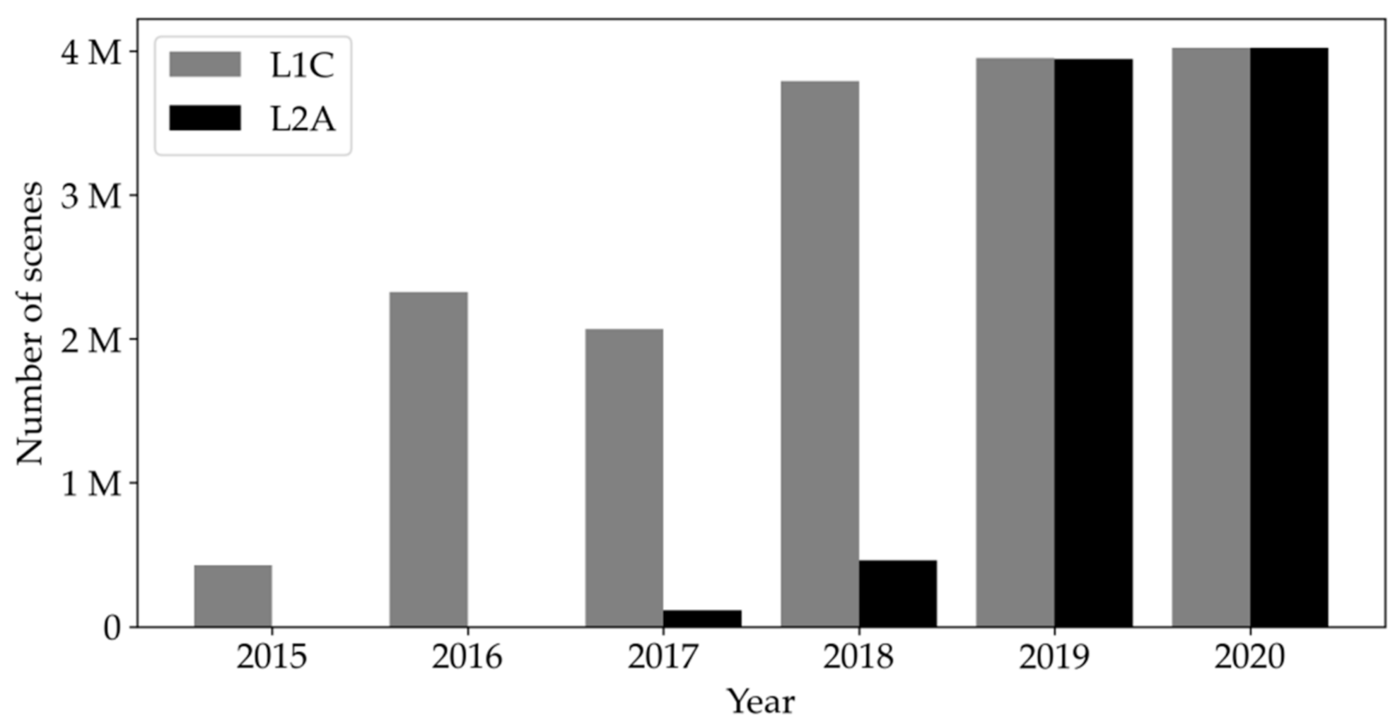
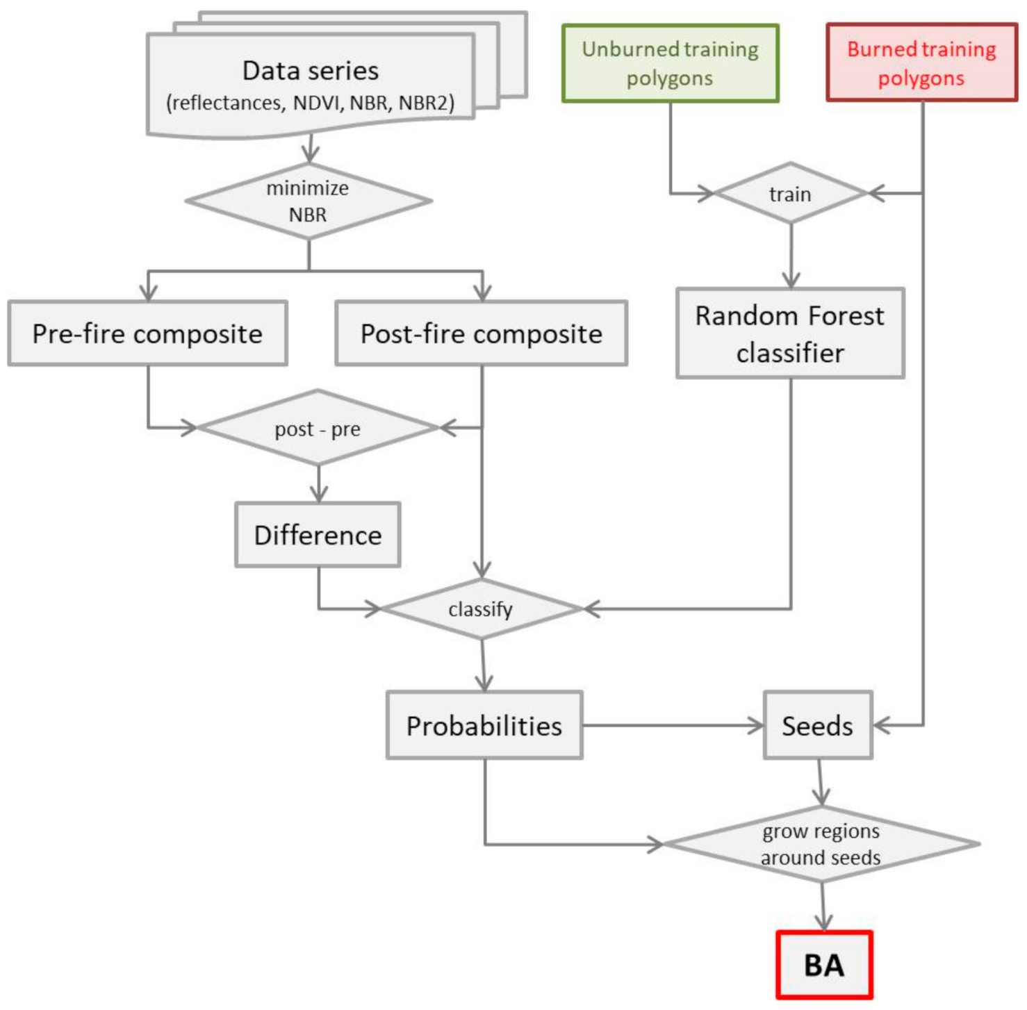
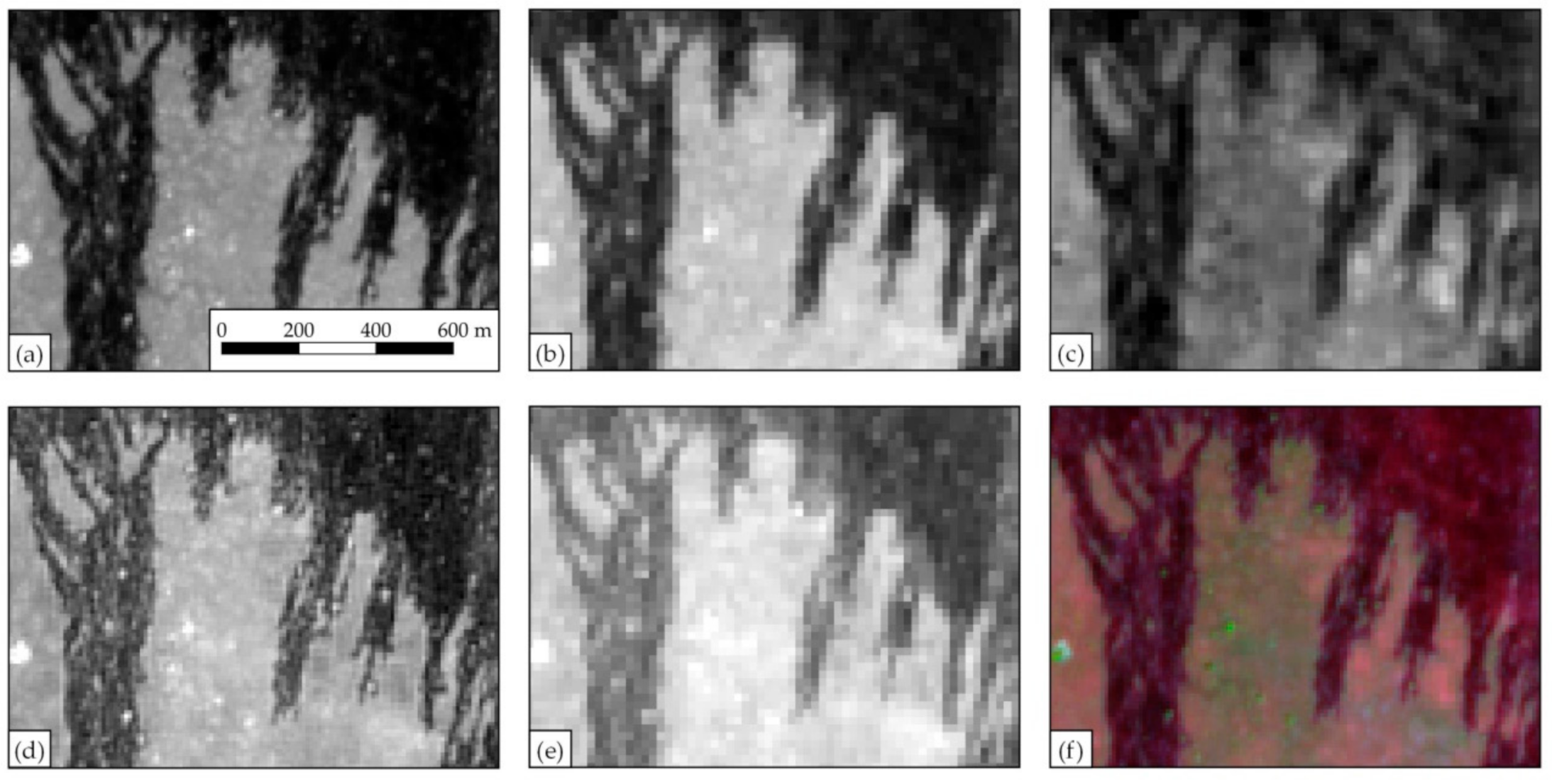
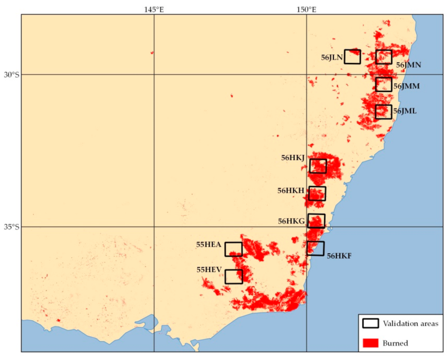
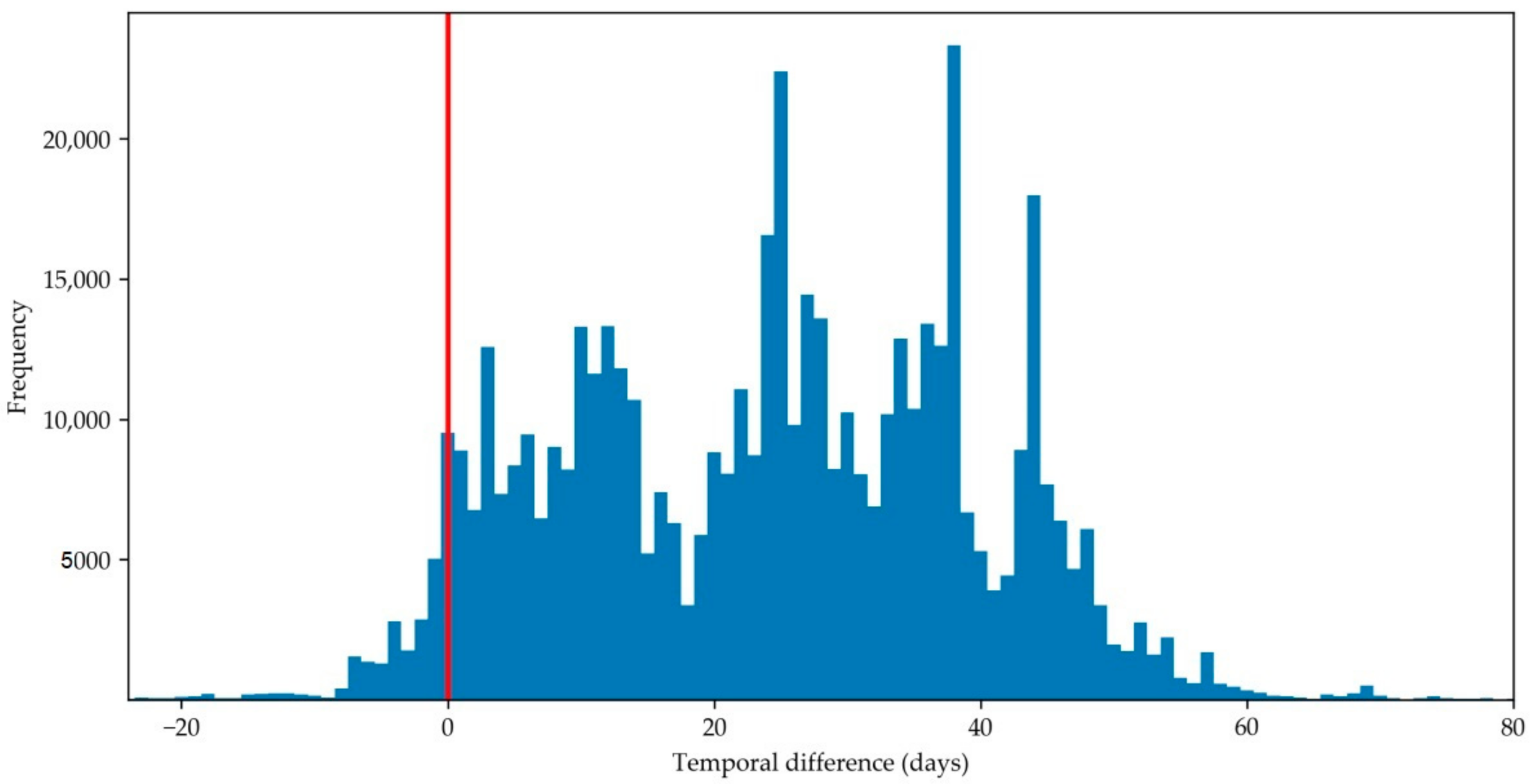
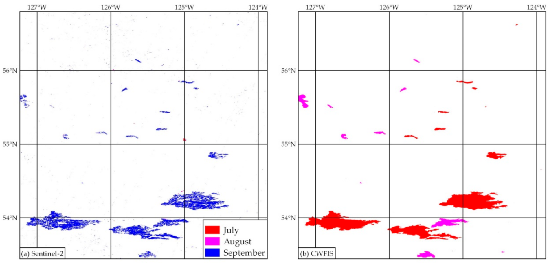
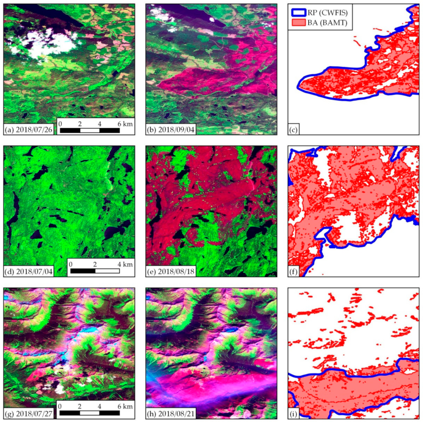
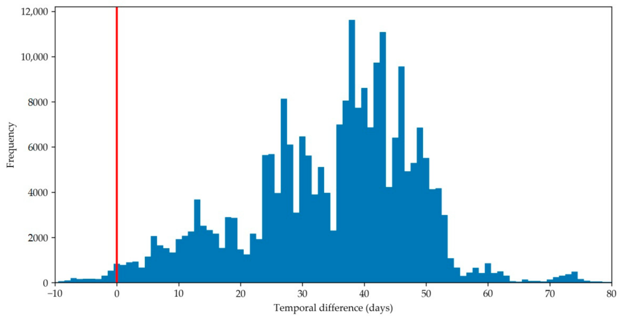
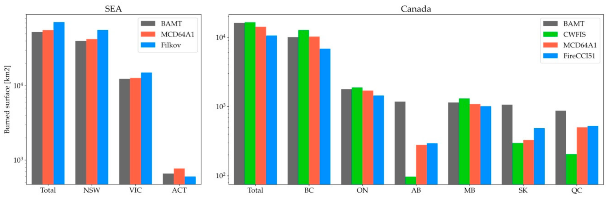
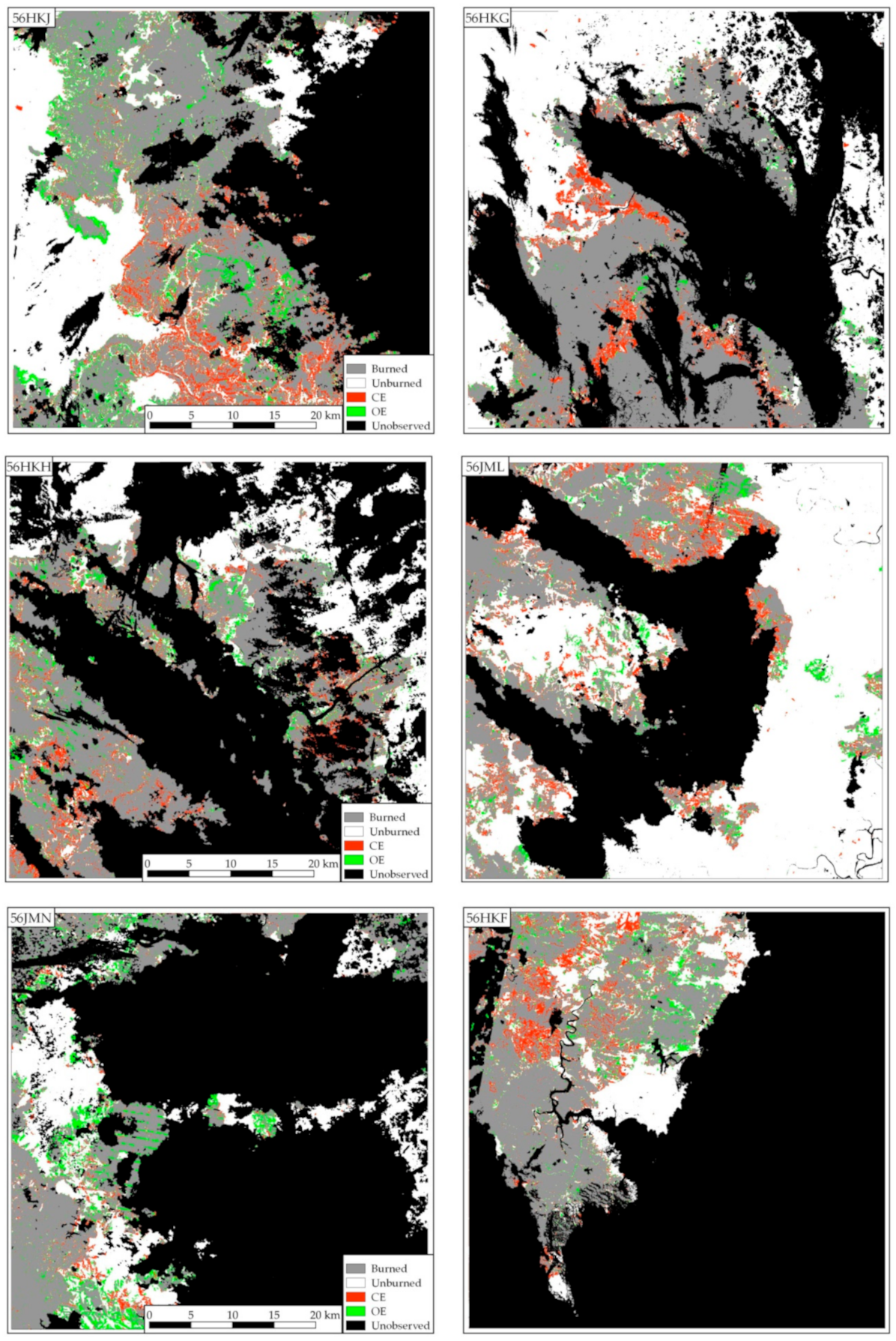
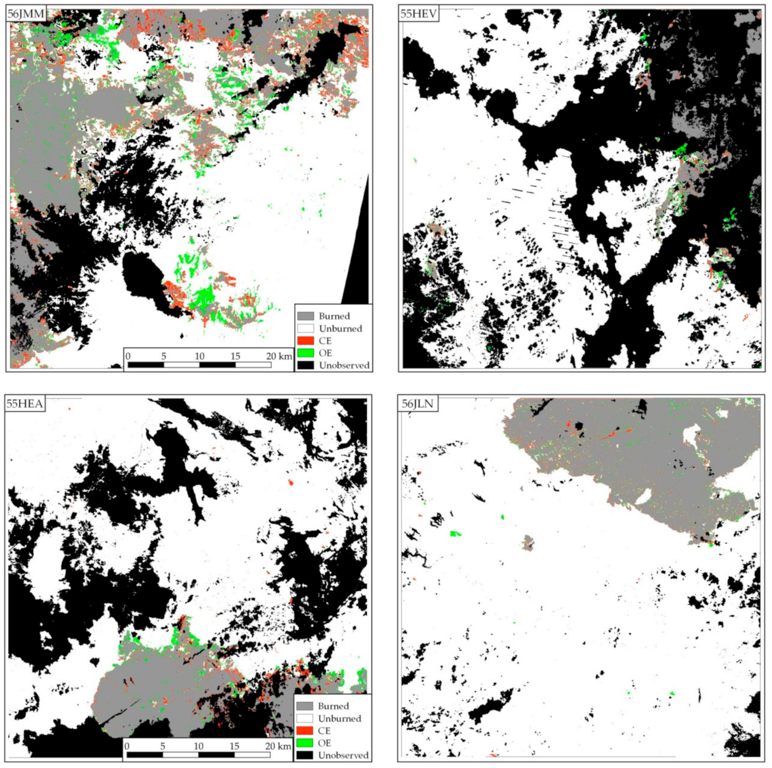
Table 1.
Selected bands for every satellite and sensor, and their approximate wavelengths.
| Satellite | Landsat-4 and 5 | Landsat-7 | Landsat-8 | Sentinel-2A and B | Approximate Wavelength (μm) |
|---|---|---|---|---|---|
| Sensor | TM | ETM + | OLI | MSI | – |
| Product | LSR | LSR | LSR | L1C | – |
| Blue | B1 | B1 | B2 | B2 | 0.45–0.52 |
| Green | B2 | B2 | B3 | B3 | 0.53–0.59 |
| Red | B3 | B3 | B4 | B4 | 0.63–0.68 |
| NIR | B4 | B4 | B5 | B8 (20 m)/B8A (30 m) | 0.80–0.89 |
| Short SWIR | B5 | B5 | B6 | B11 | 1.55–1.70 |
| Long SWIR | B7 | B7 | B7 | B12 | 2.10–2.30 |
| Quality band | pixel_qa | pixel_qa | pixel_qa | QA60 | – |
SWIR, short wavelength infrared.
Table 2.
Values and conditions applied for masking clouds and cloud shadows, depending on the dataset.
Table 2.
Values and conditions applied for masking clouds and cloud shadows, depending on the dataset.
| Landsat-4 to 8 | Sentinel-2 L1C | Sentinel-2 L2A |
|---|---|---|
| pixel_qa: 3rd bit (cloud shadow)5th bit (cloud) | QA60: 10th bit (opaque cloud) 11th bit (cirrus cloud) B1 > 1500 | SCL: value 3 (cloud shadow) value 8 (medium probability cloud) value 9 (high probability cloud) value 10 (thin cirrus) B1 > 2000 |
Table 3.
The number of training polygons, iterations, exporting time needed and number of images processed over each period in Southeast Australia (SEA) and Canada.
Table 3.
The number of training polygons, iterations, exporting time needed and number of images processed over each period in Southeast Australia (SEA) and Canada.
| Post-Fire Period | Number of Training Polygons | Iterations | Processing Time (Hours) | Number of Images | |
|---|---|---|---|---|---|
| Burned | Unburned | ||||
| 1 September–31 October 2019 | 26 | 15 | 20 | 11.0 | 938 |
| 1 November–31 December 2019 | 9 | 4 | 10 | 29.0 | 936 |
| 1 January–29 February 2020 | 10 | 8 | 9 | 14.5 | 910 |
| 1 March–30 April 2020 | 7 | 7 | 6 | 10.5 | 869 |
| Aggregated period | 52 | 34 | 45 | 64.0 | 3653 |
| 1 July–30 September 2018 (Canada) | 9 | 10 | 11 | 244.4 | 254,660 |
Table 4.
Sampled validation areas, their validation periods and validation results. All accuracy measures (commissions, omissions and Dice coefficients) are expressed in percentages.
Table 4.
Sampled validation areas, their validation periods and validation results. All accuracy measures (commissions, omissions and Dice coefficients) are expressed in percentages.
| Tile | Validation Period | Accuracy | |||||
|---|---|---|---|---|---|---|---|
| Start | End | Length in Days | Number of Images | CE | OE | DC | |
| 56HKJ | 2019/09/02 | 2020/02/19 | 170 | 10 | 13.6 | 10.8 | 87.8 |
| 56HKG | 2019/09/22 | 2020/02/29 | 160 | 8 | 10.6 | 2.9 | 93.1 |
| 56HKH | 2019/09/02 | 2020/02/19 | 170 | 9 | 11.4 | 8.0 | 90.3 |
| 56JML | 2019/09/03 | 2020/01/21 | 140 | 9 | 19.2 | 10.3 | 85.0 |
| 56JMN | 2019/09/02 | 2020/01/10 | 130 | 11 | 7.2 | 16.4 | 87.9 |
| 56HKF | 2019/09/07 | 2020/02/29 | 175 | 8 | 14.6 | 7.6 | 88.8 |
| 56JMM | 2019/09/02 | 2020/01/21 | 140 | 12 | 13.9 | 13.5 | 86.3 |
| 55HEV | 2019/09/10 | 2020/02/22 | 165 | 8 | 7.2 | 10.5 | 91.1 |
| 55HEA | 2019/09/10 | 2020/01/18 | 130 | 9 | 5.6 | 6.1 | 94.1 |
| 56JLN | 2019/09/02 | 2020/01/10 | 130 | 11 | 3.3 | 3.0 | 96.9 |
| Aggregated | – | – | – | – | 11.8 | 8.9 | 89.6 |
CE, commission error; OE, omission error; DC, Dice coefficient.
Table 5.
Total burned surface by province in Canada according to the BA product and Canadian Wildland Fire Information System (CWFIS) perimeters, and the common BA between both, expressed in square kilometers.
Table 5.
Total burned surface by province in Canada according to the BA product and Canadian Wildland Fire Information System (CWFIS) perimeters, and the common BA between both, expressed in square kilometers.
| Province | BAMT | CWFIS | Common BA |
|---|---|---|---|
| BC | 10,069 | 12,711 | 7633 |
| ON | 1778 | 1881 | 1142 |
| AB | 1175 | 97 | 83 |
| MB | 1146 | 1309 | 755 |
| SK | 1061 | 297 | 222 |
| QC | 868 | 205 | 151 |
| NL | 58 | 0 | 0 |
| NB | 5 | 0 | 0 |
| NS | 2 | 0 | 0 |
| PE | 2 | 0 | 0 |
| TOTAL | 16,165 | 16,501 | 9986 |
BAMT, Burned Area Mapping Tool; BC, British Columbia; AB, Alberta; SK, Saskatchewan; MB, Manitoba; ON, Ontario; QC, Québec; NL, Newfoundland and Labrador; PE, Prince Edward Island; NS, Nova Scotia; and NB, New Brunswick.
Publisher’s Note: MDPI stays neutral with regard to jurisdictional claims in published maps and institutional affiliations. |
© 2021 by the authors. Licensee MDPI, Basel, Switzerland. This article is an open access article distributed under the terms and conditions of the Creative Commons Attribution (CC BY) license (http://creativecommons.org/licenses/by/4.0/).
Share and Cite
MDPI and ACS Style
Roteta, E.; Bastarrika, A.; Franquesa, M.; Chuvieco, E. Landsat and Sentinel-2 Based Burned Area Mapping Tools in Google Earth Engine. Remote Sens. 2021, 13, 816. https://doi.org/10.3390/rs13040816
AMA Style
Roteta E, Bastarrika A, Franquesa M, Chuvieco E. Landsat and Sentinel-2 Based Burned Area Mapping Tools in Google Earth Engine. Remote Sensing. 2021; 13(4):816. https://doi.org/10.3390/rs13040816
Chicago/Turabian StyleRoteta, Ekhi, Aitor Bastarrika, Magí Franquesa, and Emilio Chuvieco. 2021. "Landsat and Sentinel-2 Based Burned Area Mapping Tools in Google Earth Engine" Remote Sensing 13, no. 4: 816. https://doi.org/10.3390/rs13040816
Note that from the first issue of 2016, this journal uses article numbers instead of page numbers. See further details here.