2.1 Site and sampling description

The study was conducted in the Batang Ai hydroelectric reservoir in Sarawak, Malaysia (latitude 1.16^∘ and longitude 111.9^∘). The reservoir is located in Borneo in a tropical equatorial climate with a constantly high temperature averaging 23 and 32 ^∘C during nighttime and daytime respectively (Sarawak Government, 2019). The region experiences two weak monsoon seasons (November to February and June to October) with a yearly average rainfall of 3300 to 4600 mm (Sarawak Government, 2019). The reservoir was impounded in 1985 with a dam wall of 85 m, a surface area of ∼68.4 km², and a watershed area of 1149 km² of mostly undisturbed forested land (limited rural habitations and small-scale croplands).

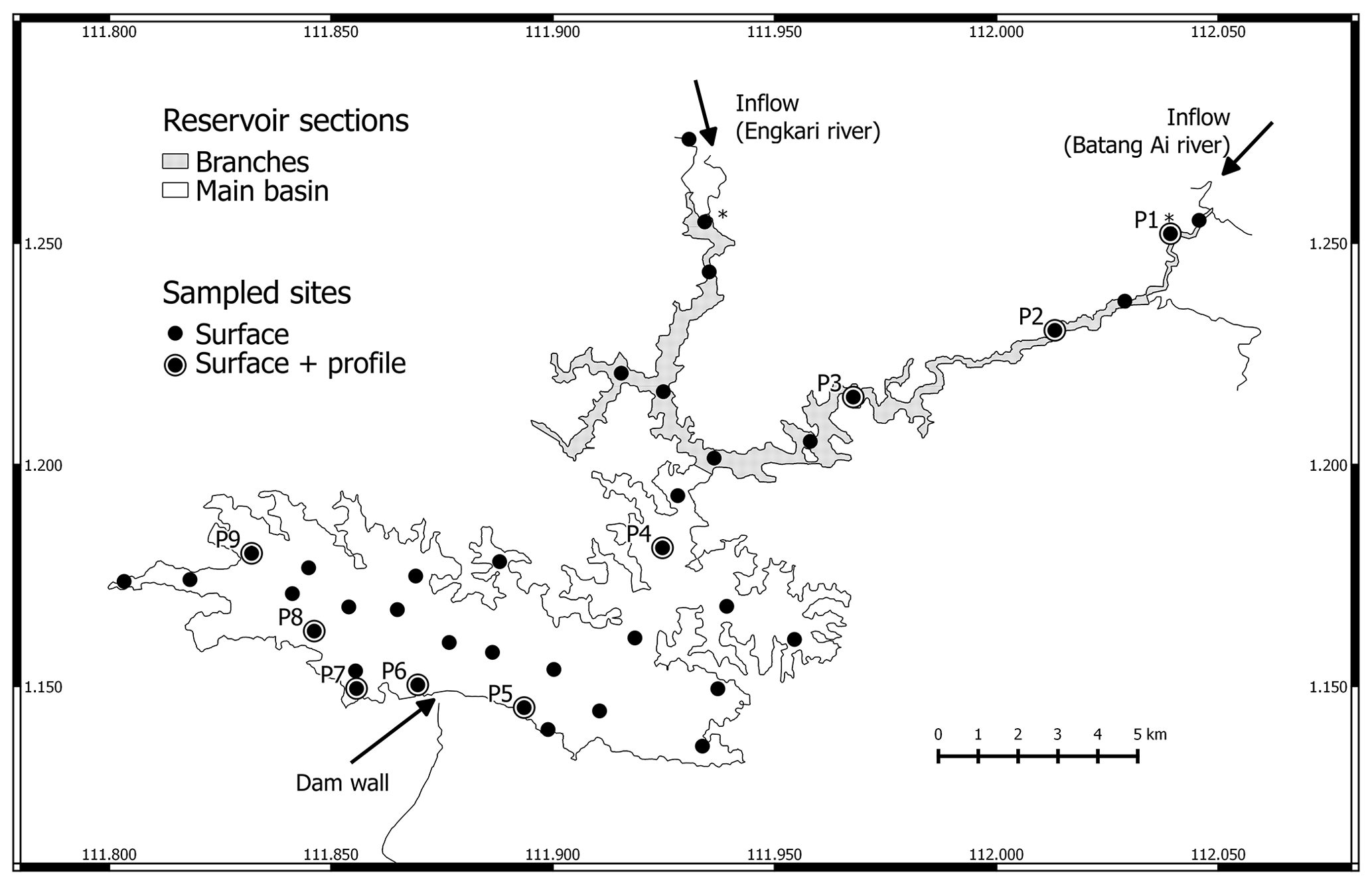
Figure 1Map of Batang Ai reservoir with delimited sections (branches and main basin) and sampling points. ^* Represents sampling points at the branches' extremities.

We distinguish between three sections of the study site: inflows, reservoir branches, and the reservoir main basin shown in Fig. 1. The inflows are the two main reservoir inlets: the Batang Ai and Engkari rivers (3 to 10 m deep where sampled). The two rivers flow into two arms that we refer to as the reservoir branches (10.8 km², mean and max depths of 18 and 52 m respectively). The reservoir branches merge into the main basin of the reservoir (58.9 km², mean and max depths of 30 and 73 m respectively). Surface sampling was performed at 36 sites across the three study sections, and water column profile sampling (from 0 up to 32 m, each 0.5 to 3 m) was done at nine sites in the reservoir branches and main basin (Fig. 1). Sampling was repeated (with a few exceptions) during four campaigns: (1) 14 November to 5 December 2016 (November–December 2016), (2) 19 April to 3 May 2017 (April–May 2017), (3) 28 February to 13 March 2018 (February–March 2018), and (4) 12 to 29 August 2018 (August 2018).

2.2 Physical and chemical analyses

Water temperature, dissolved oxygen, and pH were measured using a multi-parameter probe (YSI model 600XLM-M) equipped with a depth gauge and attached to a 12 V submersible pump (Proactive Environmental Products model Tornado) for water sample collection. Concentrations of dissolved organic carbon (DOC), total phosphorus (TP), total nitrogen (TN), and chlorophyll a (chl a) were measured during all campaigns at all surface sampling sites (Fig. 1). Methods for these analyses are described in detail in Soued and Prairie (2020). Briefly, TP and chl a (extracted with hot ethanol) were analyzed via spectrophotometry, and TN and DOC (filtered at 0.45 µm) were measured on an Alpkem Flow Solution IV autoanalyzer and on a total organic carbon analyzer 1010-OI respectively.

For each site, we defined the depths of the thermocline and the top and bottom of the metalimnion based on measured temperature profiles using the R package rLakeAnalyzer (Winslow et al., 2018). The epilimnion was defined from the surface to the top of the metalimnion and was assumed to be a mixed layer.

2.3 Gas concentration, isotopic signature, and water–air fluxes

CO₂ and CH₄ gas concentrations and isotopic signatures (δ¹³C) were measured in duplicates at the surface at 36 sites and along vertical profiles at nine sites (P1 to P9, Fig. 1) using the headspace technique described in detail in Soued and Prairie (2020). In brief, sampling was done by equilibrating the water sample for 2 min with an air headspace inside a 60 mL syringe. The gas phase was then injected in a 12 mL pre-vacuumed airtight vial and analyzed on a gas chromatograph (Shimadzu GC-8A with a flame ionization detector) for gas concentrations and on a cavity ring-down spectrometer (CRDS) equipped with a small sample isotopic module (SSIM, Picarro G2201-i) for δ¹³CO₂ and δ¹³CH₄.

Surface gas flux data used in this study are described in more detail in Soued and Prairie (2020), a previous study on the C footprint of Batang Ai reservoir. Surface diffusive fluxes of CO₂ and CH₄ were measured at all surface sampling sites during each campaign. Flux rates were derived from linear changes in CO₂ and CH₄ concentrations in a static floating chamber (design described in Soued and Prairie, 2020 and IHA, 2010) connected in a closed loop to a portable gas analyzer (model UGGA, from Los Gatos Research). Measured gas concentrations, isotopic signature, and fluxes were spatially interpolated to the whole reservoir area by inverse distance weighting (given the absence of a suitable variogram for kriging) using package gstat version 1.1-6 in the R version 3.4.1 software (Pebesma, 2004). Mean values were calculated for each campaign based on the interpolated maps (Soued and Prairie, 2020).

2.4 Horizontal GHG inputs

In order to estimate the external horizontal inputs of CO₂ and CH₄, we considered that the total volume of water inflow and outflow (discharge measured at the dam) were equal and equivalent to the mean of measured daily discharge (Q, in m³ d⁻¹) during each campaign (considering minimal changes in inflow and outflow rates during a campaign). The approach of using discharge as a measure of total water inflow has the advantage of integrating all external flow (rivers, lateral soils, and groundwater) as water inputs to the reservoir. However, the fraction of inflow feeding the reservoir surface vs. bottom layer and its average gas concentration can only be approximated based on measurements from the two main river inlets (Fig. 1) due to the lack of data on other lateral inflows. Given that part of the inflowing water is colder and denser than the reservoir surface layer, only a fraction of it enters the epilimnion of the reservoir branches, and the rest plunges into the hypolimnion. We estimated that fraction (f_epi) based on temperature profiles in the eastern river delta and branch (sites P1 and P2, Fig. 1), and we assumed it is representative of other water inflows to the reservoir. The areal rate of horizontal CO₂ and CH₄ inputs (H, in $\mathrm{mmol}{\mathrm{m}}^{-\mathrm{2}}{\mathrm{d}}^{-\mathrm{1}}$) over each section of the reservoir were then calculated following Eq. (1):

with A (m²) the surface area of the reservoir section considered and C_in (mmol m⁻³) the concentration of gas in the inflowing water. To estimate gas inputs from the inflows to the branches, C_in was considered to be the average of gas concentrations measured at the two upstream extremities of the branches (Fig. 1). To estimate gas inputs from the branches to the main basin, C_in was considered to be the gas concentrations measured at the confluence between the two branches (right upstream of the main basin).

2.5 Vertical GHG fluxes

We estimated CO₂ and CH₄ fluxes from the metalimnion to the epilimnion (V) based on the vertical gas diffusivity (K_z) and the gradient in gas concentration across the epilimnion–metalimnion interface using Eq. (2) (Wüest and Lorke, 2009):

where C_meta and C_epi are the gas concentrations at the top of the metalimnion and at the bottom of the epilimnion respectively, measured at profile sites (P1 to P9, Fig. 1). K_z was derived from the following Eq. (3) (Osborn, 1980):

where Γ is the mixing ratio set to 0.2 (Oakey, 1982), ϵ is the dissipation rate of turbulent kinetic energy, and N² is the buoyancy frequency. N² was calculated from measured temperature profiles (YSI probe) using the function buoyancy.freq from the rLakeAnalyzer package (Winslow et al., 2018) in the R software (R Core Team, 2017). ϵ was derived from measured vertical shear microstructure profiles performed in the August 2018 campaign at all profile sites shown in Fig. 1 (except P1 due to floating logs). Shear profiles were measured with a high-frequency (512 Hz) MicroCTD profiler (Rockland Scientific) equipped with two velocity shear probes, two thermistors, tilt and vibration sensors, and a pressure sensor. At each site, the profiler was cast 10 times, five with an uprising configuration (from bottom to top of the water column) and five with a downward configuration (top to bottom), with a 4 min waiting time between profiles to allow water column disturbance to subside. Data quality check and ϵ calculation for each profile cast were performed with the ODAS v4.3.03 MATLAB library (developed by Rockland Scientific) based on Nasmyth shear spectrum (Oakey, 1982), with ϵ values averaged among the two shear probes and binned over 1–2 m segments along the profile. For each site, continuous ϵ profiles were interpolated by fitting a smooth spline through all ϵ values from replicate casts as a function of depth.

At the epilimnion–metalimnion interface (top of the metalimnion ±2 m), calculated ϵ averaged $\mathrm{7.7}\times {\mathrm{10}}^{-\mathrm{9}}$ (range from $\mathrm{3.4}\times {\mathrm{10}}^{-\mathrm{9}}$ to $\mathrm{1.6}\times {\mathrm{10}}^{-\mathrm{8}}$) m² s⁻³ across all sites sampled with the MicroCTD, with no significant difference between the main basin and branch sites. In order to estimate vertical gas diffusion, we applied the latter ϵ average to Eqs. (2) and (3) for all measured gas profiles (except P1). The resulting V values for each gas were averaged across sites in the main basin and branches separately to derive estimates of V for each of these two reservoir sections.

2.6 Sediment GHG inputs

We calculated CO₂ and CH₄ inputs from the sediments to epilimnetic waters using gas profiles in sediment cores collected in April–May 2017 and February–March 2018 at seven sites (P1 to P3 in the reservoir branches and P4, P5, P7, and P9 in the main basin, Fig. 1). Sediment cores were collected using a Glew gravity corer attached to a 6 cm wide plastic liner. The liner was predrilled with 1 cm holes covered with electric tape at each centimetre up to 40 cm. Upon recovery of the sediment core, 3 mL tip-less syringes were inserted into each hole to extract sediments from each centimetre. The sediment content of each syringe was emptied into a 25 mL glass vial prefilled with 6 mL nano-pure water and immediately airtight sealed by a butyl rubber stopper crimped with an aluminum cap. Glass vials were pressurized with 40 mL of ambient air using a plastic syringe equipped with a needle to pierce the rubber cap. Glass vials were shaken for 2 min for equilibration before extracting the gas with a syringe and injecting it into a pre-evacuated airtight vial for analysis of CO₂ and CH₄ concentrations and isotopic signatures as described above. Additionally, samples of the water overlaying the sediments (∼1 cm above) were collected for similar analyses of CO₂ and CH₄.

Sediment CO₂ and CH₄ flux rates to the overlaying water column were derived from the vertical gradient of gas concentration measured in the sediment cores and overlaying water. The slope of CO₂ or CH₄ concentration as a function of depth (g, in $\mathrm{\mu }\mathrm{mol}{\mathrm{L}}^{-\mathrm{1}}{\mathrm{m}}^{-\mathrm{1}}$) was calculated for measured values in the first 5 cm of sediments and overlaying water. Most cores exhibited clear linear slopes (p value < 0.05 and $R_{\text{adj}}^{\mathrm{2}}>\mathrm{0.5}$). In the few cases where a linear slope was not evident, g was replaced by the gradient between the mean gas concentration in the first 3 cm of sediments and the overlaying water. The sediment gas flux rate (S_f in $\mathrm{mmol}{\mathrm{m}}^{-\mathrm{2}}{\mathrm{d}}^{-\mathrm{1}}$) was calculated with Eq. (4):

with d the diffusion coefficient set to $\mathrm{1.5}\times {\mathrm{10}}^{-\mathrm{5}}$ cm² s⁻¹ (Donis et al., 2017) and p the sediment porosity assumed to be 2 % based on previous results in Batang Ai (Tan, 2015).

At an ecosystem scale, sediment CO₂ and CH₄ inputs to the water column (S) were estimated based on average and standard deviation values of sites located in each section of the reservoir (branches and main basin). For each section, mean sediment CO₂ and CH₄ flux rates were multiplied by the areal ratio of epilimnetic sediments (A_epi) vs. total water area (A₀). The latter ratio was calculated based on the hypsometric model (Ferland et al., 2014; Imboden, 1973) as shown in Eqs. (5) to (7):

with q a parameter describing the general bathymetric shape of the reservoir section, z_max and z_mean the maximum and mean depths respectively, and z_epi the mean depth of the epilimnion (8.0 and 10.5 m in the branches and main basin respectively).

Littoral sediments are known to be a source of CH₄ not only through diffusion but also via ebullition. While this emission pathway was found to be important in other reservoirs (Deemer et al., 2016), it is surprisingly low in Batang Ai, equaling less than 2 % of CH₄ surface diffusive emissions, and only 0.1 % of the reservoir total GHG footprint (Soued and Prairie, 2020). Therefore, sediment ebullition was considered negligible in the epilimnetic CH₄ budget of Batang Ai.

2.7 Metabolic rates

Net metabolic rates of CO₂ and CH₄ production in the epilimnetic water column were estimated with in situ incubations. Incubations were performed at five sites (P2 and P3 in the branches and P4, P5, and P7 in the main basin, Fig. 1). Water from 3 m deep was pumped into 5 L transparent glass jars with an airtight clamp lid. Before closing, jars were filled from the bottom and allowed to overflow and then sampled for initial CO₂ and CH₄ concentrations. Closed jars were fixed at 3 m to an anchored line at the sampling site and incubated in in situ temperature and light conditions for 22.0 to 24.2 h. Upon retrieval, samples of final CO₂ and CH₄ concentrations were collected from the jars. Volumetric daily rates of net CO₂ and CH₄ production were calculated based on the difference between final and initial gas concentrations rescaled to a 24 h period.

In addition to incubations, open-water high-frequency O₂ measurements were carried out to derive CO₂ metabolism on larger spatial and temporal scales. Rates of GPP, ER, and net ecosystem production (NEP) were estimated in the reservoir surface layer by monitoring and inverse modelling diel O₂ changes in the epilimnion. O₂ was measured at a 1 min interval using high-frequency O₂ and temperature sensors (model miniDOT from Precision Measurement Engineering), along with light sensors (model HOBO Pendant from Onset). Sensors were deployed in profile sites P1 to P3 in the branches and P4, P5, P7, and P9 in the main basin (Fig. 1). Note that not all sites were sampled in all sampling campaigns. Sensors were attached to an anchored line at a depth between 0.7 and 3 m and deployment time varied between 4 d and 2 weeks. Upon retrieval of the sensors, the first data quality check and selection were made based on the sensor internal quality index and visual screening. Rates of ecosystem metabolism were then estimated based on an open-system diel O₂ model (Odum, 1956), where change in O₂ concentration is a function of GPP, ER, and air–water gas exchange ($K_{{\mathrm{O}}_{\mathrm{2}}}$) following Eq. (8) (Hall and Hotchkiss, 2017):

with O_2sat the theoretical O₂ concentration at saturation considering the in situ temperature and atmospheric pressure, and O₂ is the actual measured O₂ concentration in the water. A detailed description of the model equations can be found in Hall and Hotchkiss (2017). Daily estimates of GPP, ER, and K₆₀₀ (based on $K_{{\mathrm{O}}_{\mathrm{2}}}$) were derived by maximum likelihood fitting of the data to the model in Eq. (8) using the R package StreamMetabolizer (Appling et al., 2018). Note that even though the package used was originally developed for streams, it is easily transferable to lakes given that the model used (Eq. 8) is generalized for all water bodies, with the parameter z_epi describing the depth of a mixed water column of either a lentic or lotic system and with the K₆₀₀ estimate relying only on data fitting to the model and not on system type. In some cases, where the best predicted K₆₀₀ was negative, the fitting process was rerun with a user-defined positive K₆₀₀, either equal to a value estimated for the previous or subsequent day at the same site (range of 0.03–0.96 d⁻¹) or fixed to 0.1 d⁻¹ (if there is no other available estimate). When considering the epilimnion depth, predicted values of K₆₀₀ translate into a first to third quantile range of 1.17 to 5.55 m d⁻¹, which is similar to the range of K₆₀₀ values back-calculated from surface gas flux measurements with the floating chamber technique. A final selection of daily metabolic estimates was done based on the model goodness of fit assessed by calculating Pearson correlation coefficient between modelled and measured O₂ values and discarding days with a correlation lower than 0.9. Based on GPP and ER estimates, we calculated daily NEP as the balance between these two processes, and we converted it to net CO₂ production rate by assuming an O₂:CO₂ metabolic quotient of 1.

Areal metabolic rates were derived by integrating volumetric rates over the depth of the epilimnion. Average estimates of areal metabolic rates per campaign were obtained for the branches and main basin by first averaging data within each site and then across sites for each reservoir section. Note that one value derived from incubations was excluded from the calculation of the average net CH₄ production rate in the branches due to its high value of initial CH₄ concentration (an order of magnitude higher than in all other incubations and all epilimnetic data from this site). The high CH₄ concentration, unrepresentative of real conditions, was probably caused by CH₄ contamination during sampling and triggered a high oxidation rate that would overestimate the real ecosystem average rate if included.

2.8 Epilimnetic GHG budgets

Areal rates of horizontal, vertical, sediment, and metabolic inputs were combined into a sum of sources and sinks and compared to the rate of surface gas flux for each gas in each reservoir section. A mean and standard error were calculated for every component of the budgets based on measurements averaged across sites and/or sampling campaigns in order to obtain ecosystem-scale estimates of the component means and uncertainties. In the case of CO₂ metabolism, the ecosystem-scale average was calculated as the mean of the two average values derived from the incubation and diel O₂ monitoring methods. For every component, density curves were derived considering a normal distribution based on the mean and its standard error in order to visualize the relative magnitude and uncertainty of each ecosystem-scale areal rate (Fig. 3).

3.1 Physical and chemical properties

Surface water temperature exhibited a marked increase from the inflows to the branches, averaging 27.1 and 30.7 ^∘C respectively (Table 1). There was no difference in surface water temperature between the branches and the main basin. The depth of the epilimnion tended to increase and become more stable along the water flow, going from 1.3 (±1.6) m in the Batang Ai River delta to 8.0 (±2.3) m in its branch and 10.6 (±1.7) m in the main basin (Table 1). Light penetration exhibited the same spatial pattern, with an increasing Secchi depth along the water flow averaging 1.3, 5.1, and 5.5 m in the inflows, branches, and main basin respectively (Table 1). All sections of the study system exhibited oligotrophic water properties (Table 1).

3.2 Surface GHG concentrations, fluxes, and isotopic signatures

Surface CO₂ and CH₄ patterns are summarized in Fig. 2, presenting campaign averages of spatially interpolated gas concentration, flux, and isotopic signature along the different reservoir sections. Despite the temporal variability, the gas patterns along the water flow are robust, remaining similar throughout time (Fig. 2).

Table 1Mean (±SD) of physical and chemical variables measured at the surface of the three reservoir sections.

Download Print Version | Download XLSX

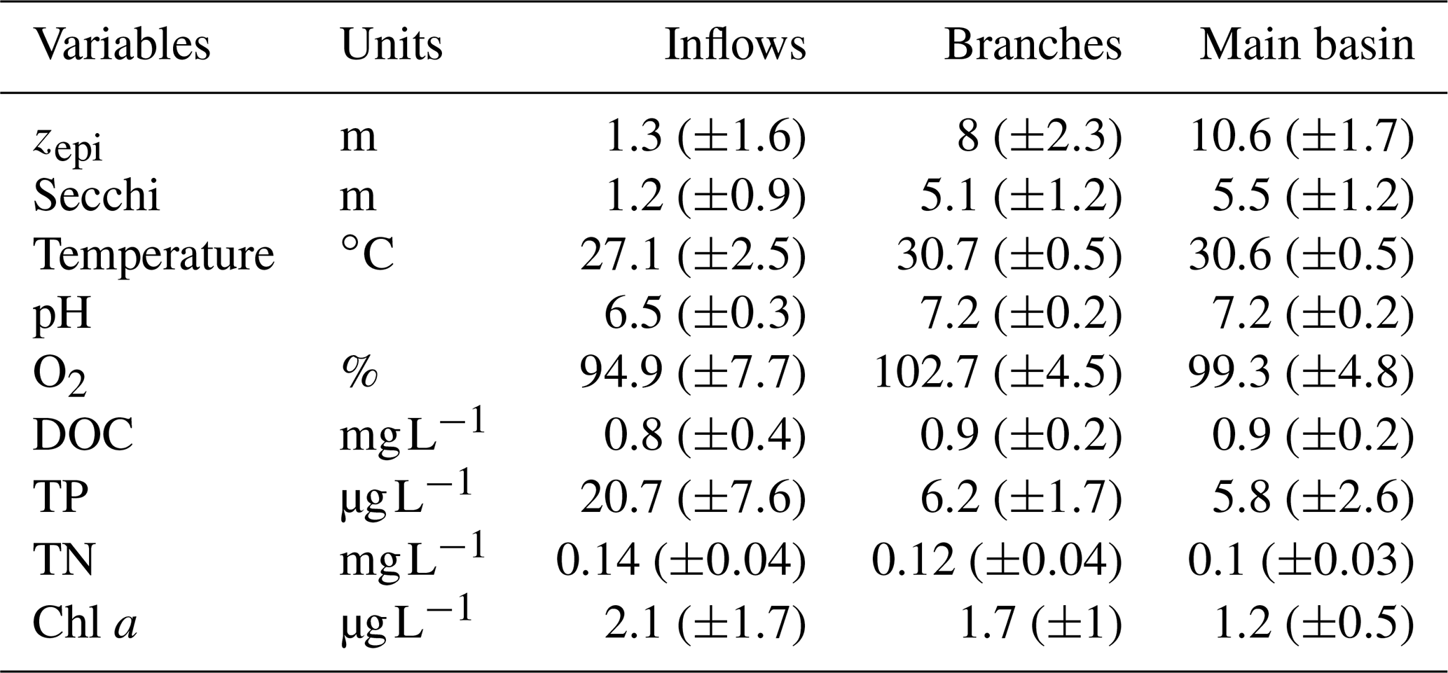
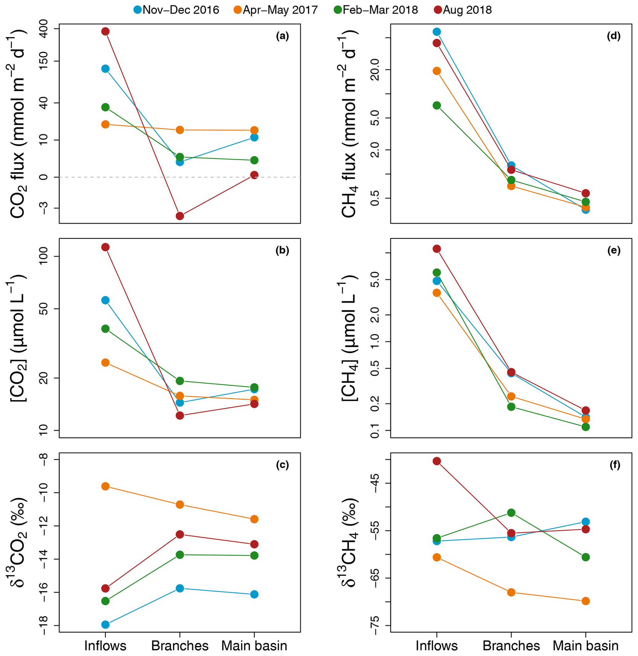
Figure 2Average of spatially interpolated surface CO₂ (a–c) and CH₄ (d–f) fluxes (a, d), concentrations (b, e), and isotopic signatures (c, f) along the hydrological continuum from the reservoir inflows to the main basin for each sampling campaign.

Download

Average CO₂ air–water flux and surface concentration were systematically higher in the inflows (mean [range]: 135.3 [18.9–368.8] $\mathrm{mmol}{\mathrm{m}}^{-\mathrm{2}}{\mathrm{d}}^{-\mathrm{1}}$ and 58.0 [24.5–113.0] µmol L⁻¹ respectively) compared to the branches (4.7 [−3.4–15.2] $\mathrm{mmol}{\mathrm{m}}^{-\mathrm{2}}{\mathrm{d}}^{-\mathrm{1}}$ and 15.4 [12.2–19.3] µmol L⁻¹) and main basin (7.5 [0.3–15.1] $\mathrm{mmol}{\mathrm{m}}^{-\mathrm{2}}{\mathrm{d}}^{-\mathrm{1}}$ and 16.0 [14.2–17.7] µmol L⁻¹) (Fig. 2a and b). Surface CO₂ concentration in the reservoir (branches and main basin) was most strongly correlated inversely with water temperature ($R_{\text{adj}}^{\mathrm{2}}=\mathrm{0.22}$, p value < 0.001, Fig. S1a and Table S1 in the Supplement). Except for the April–March 2017 campaign, there was a modest increase (2.2 ‰ to 3.3 ‰) in surface δ¹³CO₂ towards more enriched values from the inflows to the branches (Fig. 2c).

Similarly, surface CH₄ flux and concentration continually decreased along the water channel, being an order of magnitude higher in the inflows compared to the branches and about twice as high in the branches compared to the main basin (Fig. 2d and e). Of all measured water properties, TN was the most strongly linked to reservoir surface CH₄ concentration ($R_{\text{adj}}^{\mathrm{2}}=\mathrm{0.14}$, p value < 0.001, Fig. S1b and Table S1). In the main basin, surface CH₄ concentration significantly decreased with distance to shore in November–December 2016 ($R_{\text{adj}}^{\mathrm{2}}=\mathrm{0.54}$, p value < 0.001), but this correlation was weaker ($R_{\text{adj}}^{\mathrm{2}}\le \mathrm{0.13}$, p value ≥0.03) during other sampling campaigns (Fig. 6a). Surface δ¹³CH₄ values varied widely, between −83.3 and −47.6 ‰, but did not show a consistent spatial pattern (Fig. 2f) apart from a positive correlation with distance to shore in the main basin in November–December 2016 ($R_{\text{adj}}^{\mathrm{2}}=\mathrm{0.29}$, p value = 0.01, Fig. 6b).

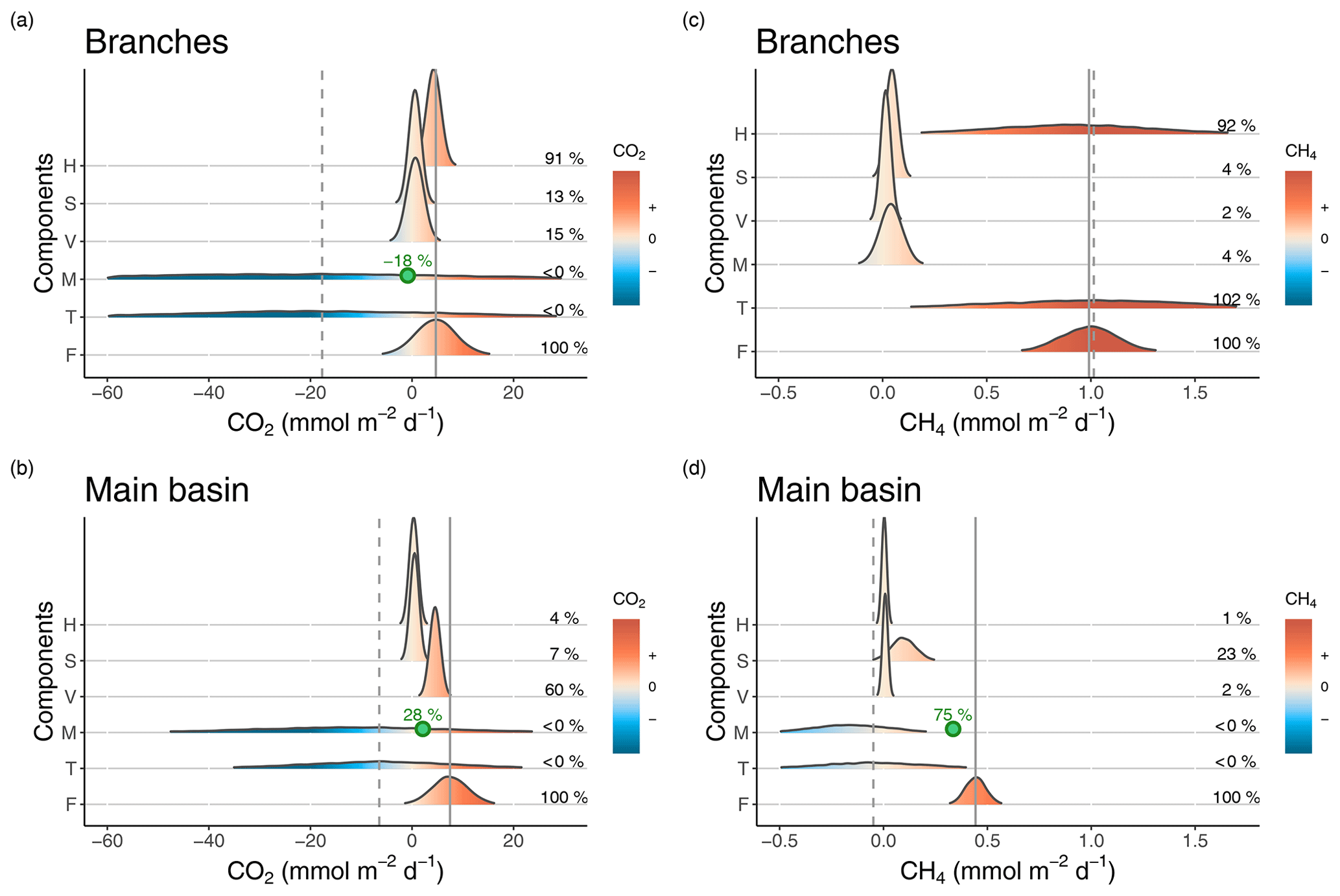
Figure 3Density distributions of the different components of CO₂ (a, b) and CH₄ (c, d) surface budgets in the reservoir branches (a, c) and main basin (b, d). Components are as follows. H: horizontal flow inputs; S: sediment inputs; V: vertical inputs; M: net metabolism (average of the incubation and diel O₂ monitoring methods); T: sum of all estimated sources and processes in the surface layer; F: measured surface fluxes. Density curves are based on simulated normal distributions using the mean and standard error of each component. The x axes represent the areal rate of CO₂ or CH₄, and the colour scale indicates the sign of the rate. Mean values of the fraction of each component (%) relative to the mean surface flux (F) are reported on the right side in each panel. The solid and dashed grey lines represent the means of F and T respectively. In panels (a), (b), and (d), the point and percentage in green represent the hypothetical value of the M rate (the most uncertain component) and its corresponding fraction (as a percentage of F) that are needed to close the budget (to obtain T = F).

Download

The degree of coupling between CO₂ and CH₄ followed a clear spatial pattern. While CO₂ and CH₄ surface concentrations were strongly linked in the inflows ($R_{\text{adj}}^{\mathrm{2}}=\mathrm{0.54}$, p value = 0.006), they became only weakly correlated in the branches ($R_{\text{adj}}^{\mathrm{2}}=\mathrm{0.17}$, p=0.005) and not correlated at all in the main basin ($R_{\text{adj}}^{\mathrm{2}}=\mathrm{0.01}$, p value = 0.11) (Fig. S2 in the Supplement).

3.3 Horizontal GHG flow

Horizontal inputs from the inflows to the surface layer of the branches were estimated to vary between 0.34–0.71 mol s⁻¹ for CO₂ and 0.02–0.25 mol s⁻¹ for CH₄. When expressed as areal rates over the branches (to facilitate comparison with other components), horizontal inputs amounted to 2.7–5.7 and 0.16–1.97 $\mathrm{mmol}{\mathrm{m}}^{-\mathrm{2}}{\mathrm{d}}^{-\mathrm{1}}$ for CO₂ and CH₄ respectively (Tables S2 and S3 in the Supplement). These values are of the same order of magnitude as surface fluxes calculated in the branches (Fig. 3a and c, Tables S2 and S3). However, the effect of horizontal inputs faded spatially, with much lower inputs from the branches to the main reservoir basin, averaging 0.31 and 0.004 $\mathrm{mmol}{\mathrm{m}}^{-\mathrm{2}}{\mathrm{d}}^{-\mathrm{1}}$ for CO₂ and CH₄ respectively (Fig. 3b and d and Tables S2 and S3). For CH₄, this fits spatial and temporal surface flux measurements, being systematically higher in the branches and maximal during the two sampling campaigns with the highest recorded horizontal inputs from the inflows (Table S3). In contrast, CO₂ surface flux was typically lower (sometimes negative) in the branches compared to the main basin, despite substantial riverine inputs to the branches (Table S2).

3.4 Vertical GHG inputs

Vertical fluxes depend on the gas diffusivity and concentration gradient. Gas diffusivity is a function of the strength of stratification (N²) and energy dissipation rate (ϵ). Measured values of N² and ϵ varied widely, from $\mathrm{5.9}\times {\mathrm{10}}^{-\mathrm{5}}$ to $\mathrm{2.3}\times {\mathrm{10}}^{-\mathrm{3}}$ s⁻² and from $\mathrm{3.4}\times {\mathrm{10}}^{-\mathrm{9}}$ to $\mathrm{1.6}\times {\mathrm{10}}^{-\mathrm{8}}$ m² s⁻³ respectively, but with no clear differences between the reservoir branches and main basin (Fig. S3a and b in the Supplement). Similarly, CO₂ and CH₄ concentration gradients varied substantially in both space and time (from −18.4 to 94.3 $\mathrm{\mu }\mathrm{mol}{\mathrm{L}}^{-\mathrm{1}}{\mathrm{m}}^{-\mathrm{1}}$ for CO₂ and −0.19 to 0.4 $\mathrm{\mu }\mathrm{mol}{\mathrm{L}}^{-\mathrm{1}}{\mathrm{m}}^{-\mathrm{1}}$ for CH₄). CO₂ concentration generally increased from the epilimnion to the metalimnion as a result of the respiratory CO₂ buildup in the deep layer. On rare occasions, an inverse gradient was observed, possibly due to autotrophic activity in the metalimnion. For CH₄, metalimnion-to-epilimnion concentration gradients were generally modest, averaging 0.04 $\mathrm{\mu }\mathrm{mol}{\mathrm{L}}^{-\mathrm{1}}{\mathrm{m}}^{-\mathrm{1}}$, and even negative in one-third of the profiles, leading to the diffusion of epilimnetic CH₄ toward deeper layers instead of the reverse. The low to negative CH₄ vertical flux results from a highly active methanotrophic layer reducing CH₄ concentration in the metalimnion, as evidenced by the strong enrichment effect observed in δ¹³CH₄ profiles (Fig. S4 in the Supplement). The combination of vertical diffusivity and gas concentration gradients resulted in vertical fluxes averaging 3.4 (−1.8 to 20.5) $\mathrm{mmol}{\mathrm{m}}^{-\mathrm{2}}{\mathrm{d}}^{-\mathrm{1}}$ for CO₂ and 0.01 (−0.01 to 0.09) $\mathrm{mmol}{\mathrm{m}}^{-\mathrm{2}}{\mathrm{d}}^{-\mathrm{1}}$ for CH₄, with no significant differences between the reservoir branches and main basin (Fig. S3).

3.5 GHG inputs from littoral sediments

Areal sediment gas fluxes ranged from 1.2 to 4.0 and −0.29 to 1.10 $\mathrm{mmol}{\mathrm{m}}^{-\mathrm{2}}{\mathrm{d}}^{-\mathrm{1}}$ for CO₂ and CH₄ respectively (Fig. S5 in the Supplement), in the range of previously reported values in lakes and reservoirs (Adams, 2005; Algesten et al., 2005; Gruca-Rokosz and Tomaszek, 2015; Huttunen et al., 2006). Sediment fluxes were not different in the branches vs. the main basin for both CO₂ (mean of 2.2 vs. 2.4 $\mathrm{mmol}{\mathrm{m}}^{-\mathrm{2}}{\mathrm{d}}^{-\mathrm{1}}$) and CH₄ (mean of 0.17 vs. 0.48 $\mathrm{mmol}{\mathrm{m}}^{-\mathrm{2}}{\mathrm{d}}^{-\mathrm{1}}$) (Fig. S5). Applying measured averages to the area of epilimnetic sediments in each section yields estimates of sediment inputs to the epilimnion of 0.6 (±0.03) and 0.5 (±0.11) $\mathrm{mmol}{\mathrm{m}}^{-\mathrm{2}}{\mathrm{d}}^{-\mathrm{1}}$ for CO₂ and 0.04 (±0.02) and 0.10 (±0.06) $\mathrm{mmol}{\mathrm{m}}^{-\mathrm{2}}{\mathrm{d}}^{-\mathrm{1}}$ for CH₄ in the branches and main basin respectively (Fig. 3 and Tables S2 and S3). These inputs from littoral sediments likely represent an upper limit since they are based on deep pelagic sediment cores (littoral area were too compact for coring), where a higher organic matter accumulation and degradation is expected (Blais and Kalff, 1995; Soued and Prairie, 2020). Even as upper estimates, the calculated rates of sediment GHG inputs remain a relatively modest fraction of the average emissions to the atmosphere for the branches and main basin for both CO₂ (13 % and 7 % respectively) and CH₄ (4 % and 23 % respectively) (Tables S2 and S3).

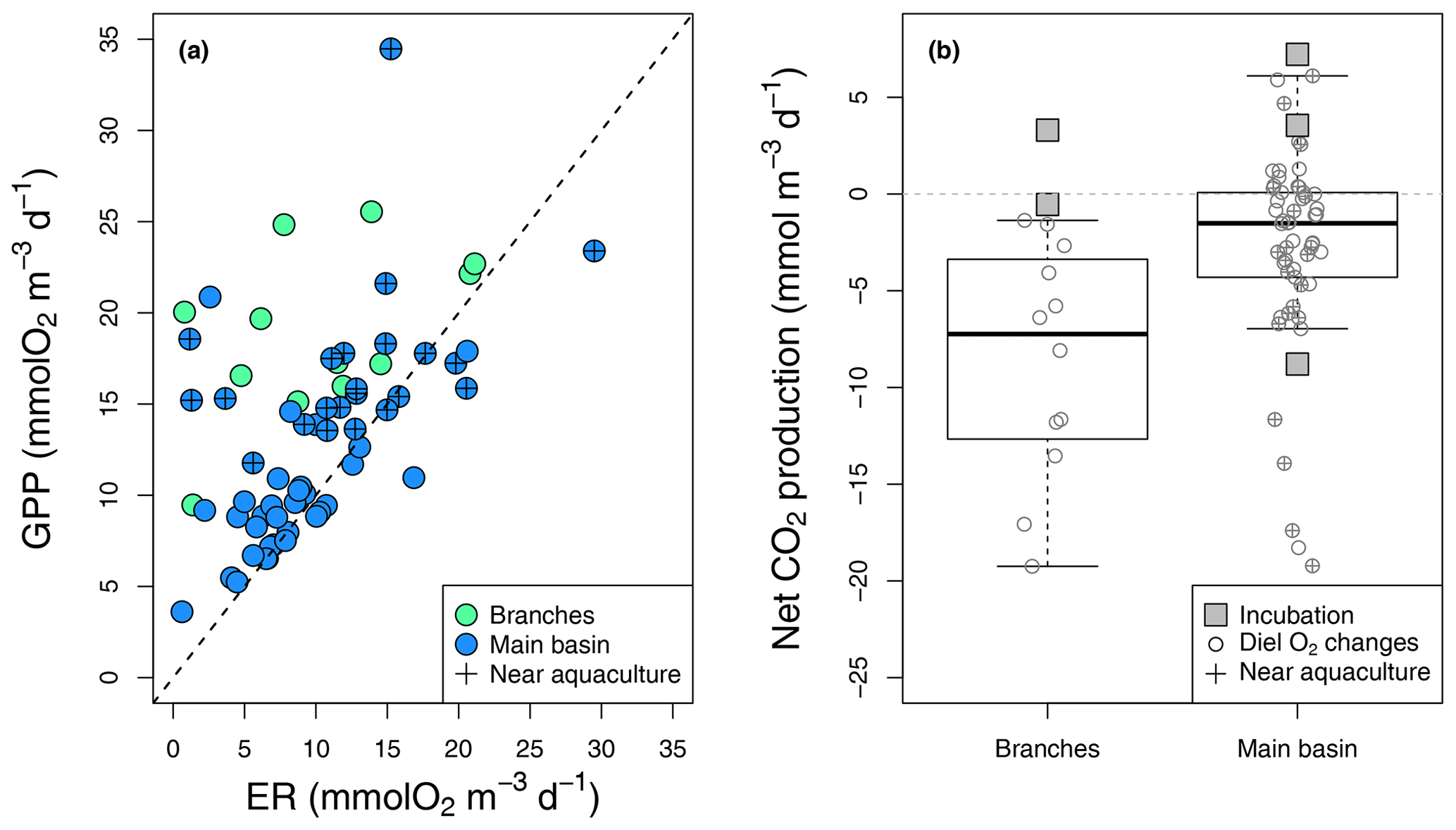
Figure 4Epilimnetic daily GPP vs. ER rates (a) derived from diel O₂ changes in the reservoir branches and main basin (including sites near aquacultures), with the 1:1 line (dotted). (b) Boxplots of the corresponding rates of CO₂ NEP in the branches and main basin, with box bounds, whiskers, solid line, open circles, and squares representing the 25th and 75th percentiles, the 10th and 90th percentiles, the median, single data points (diel O₂ method), and incubation-derived rates respectively.

Download

3.6 Metabolism

3.6.1 CO₂ metabolism

Estimated GPP and ER rates based on diel O₂ monitoring ranged from 3.6 to 34.5 $\mathrm{\mu }\mathrm{mol}{\mathrm{L}}^{-\mathrm{1}}{\mathrm{d}}^{-\mathrm{1}}$ and from 5.8 to 29.5 $\mathrm{\mu }\mathrm{mol}{\mathrm{L}}^{-\mathrm{1}}{\mathrm{d}}^{-\mathrm{1}}$ respectively (Fig. 4a), which is well within the range of reported rates for oligotrophic systems (Bogard and del Giorgio, 2016; Hanson et al., 2003; Solomon et al., 2013). As expected, GPP and ER rates were correlated ($R_{\text{adj}}^{\mathrm{2}}=\mathrm{0.23}$, p value < 0.001, Fig. 4a), with photosynthesis stimulating the respiration of produced organic matter. In most cases, GPP exceeded ER, especially in the branches and near aquacultures (Fig. 4a), where higher nutrients (TP and TN) and chl a concentrations were measured (Table 1). Daily metabolic rates showed no correlation with mean daily rain or light (Kendall rank correlation p value > 0.1).

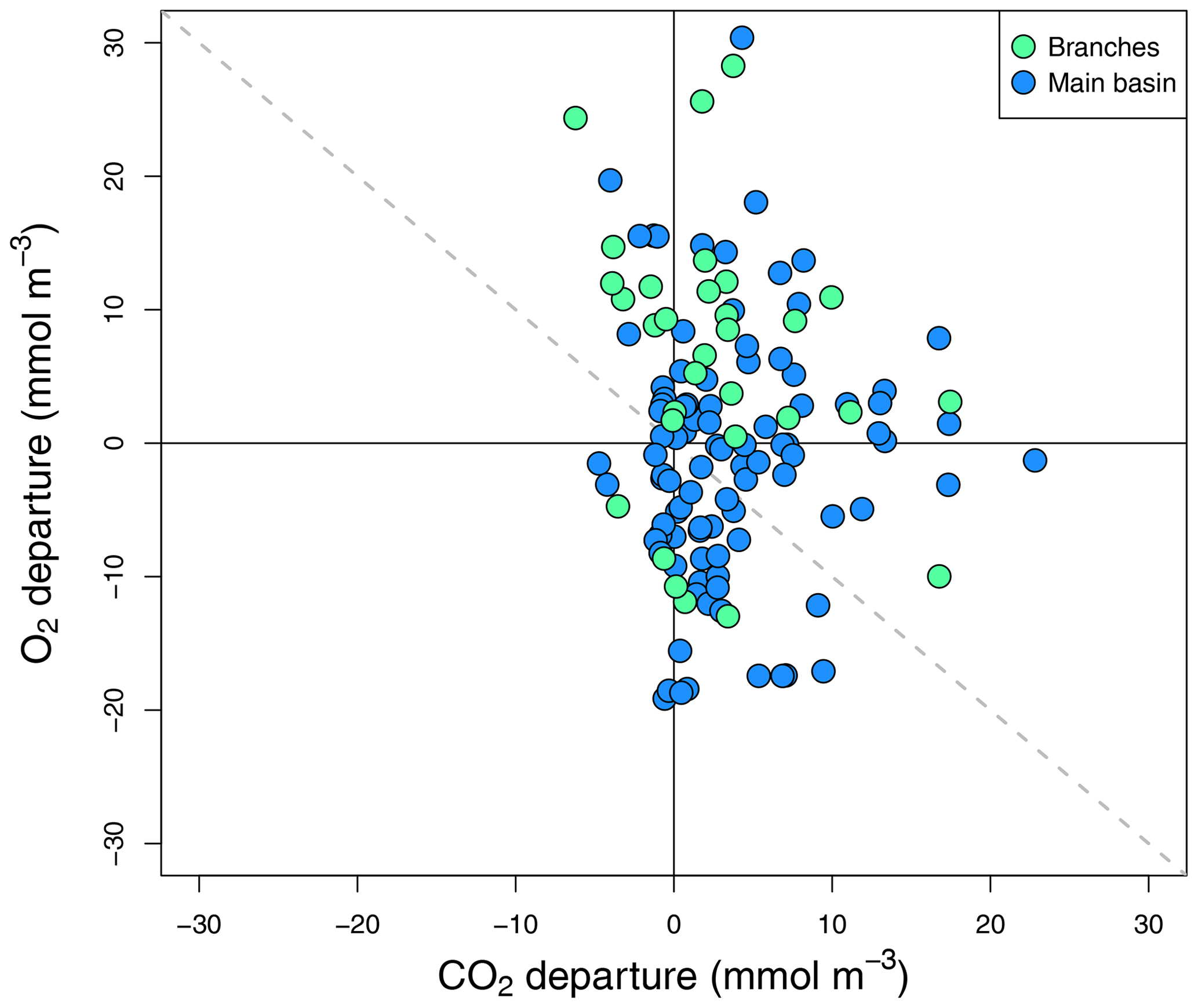
Figure 5Surface O₂ vs. CO₂ departure from saturation for all sampled surface sites in the reservoir main basin and branches across all sampling campaigns.

Download

Figure 6Regression of CH₄ concentration (a) and isotopic signature (b) as a function of distance to shore in each sampling campaign in the main reservoir basin. For CH₄ concentration, regressions lines have the following statistics in order of sampling: p values: <0.001, 0.06, 0.03, and 0.05 and $R_{\text{adj}}^{\mathrm{2}}$: 0.54, 0.13, and 0.11. For δ¹³CH₄, all regressions had p values > 0.2 except for the November–December 2016 campaign with a p value = 0.01 and $R_{\text{adj}}^{\mathrm{2}}=\mathrm{0.29}$.

Download

In the reservoir branches, results from the diel O₂ monitoring method suggested systematic net CO₂ uptake ranging from −19.2 to −1.4 $\mathrm{\mu }\mathrm{mol}{\mathrm{L}}^{-\mathrm{1}}{\mathrm{d}}^{-\mathrm{1}}$, whereas results from two incubations were slightly above that range (−0.5 to 3.3 $\mathrm{\mu }\mathrm{mol}{\mathrm{L}}^{-\mathrm{1}}{\mathrm{d}}^{-\mathrm{1}}$) (Fig. 4b). In the main basin, incubation results ranged from −8.8 to 7.2 $\mathrm{\mu }\mathrm{mol}{\mathrm{L}}^{-\mathrm{1}}{\mathrm{d}}^{-\mathrm{1}}$, while the diel O₂ technique captured a wider variability in net CO₂ metabolic rates from −19.2 to 6.1 $\mathrm{\mu }\mathrm{mol}{\mathrm{L}}^{-\mathrm{1}}{\mathrm{d}}^{-\mathrm{1}}$, with an estimated CO₂ uptake in 39 out of 54 cases (Fig. 4b). Areal net CO₂ metabolic rates, as the average of the two methods, yielded an ecosystem-scale estimate of −23.2 and −11.8 $\mathrm{mmol}{\mathrm{m}}^{-\mathrm{2}}{\mathrm{d}}^{-\mathrm{1}}$ in the reservoir branches and main basin respectively (Table S2).

To complement the metabolic rate data, surface O₂ and CO₂ departure from saturation was examined in both reservoir sections. O₂ oversaturation was observed in 44 % of cases in the main basin and 81 % in the branches (Fig. 5), which corresponds with the spatial patterns of net metabolic rates (Fig. 4b). CO₂ oversaturation was also widespread (74 % of cases), making many sampled sites oversaturated in both O₂ and CO₂ (55 % in the branches and 32 % in the main basin, Fig. 5).

3.7 Ecosystem-scale GHG budgets

Estimated sources and sinks of CO₂ and CH₄ were collated into a budget to evaluate their relative impact on epilimnetic gas concentration and to assess whether their sum matches the measured surface gas fluxes in each section of the reservoir. Figure 3 depicts such reconstruction of the epilimnetic CO₂ and CH₄ budgets in Batang Ai as well as the uncertainty limits of each component. While each process varied in time, their relative importance in driving surface fluxes was generally similar from one sampling campaign to another (Tables S2 and S3).

4.1 Spatial dynamics of CO₂ and CH₄

The decrease in gas concentration and air–water fluxes along the hydrological continuum observed across sampling campaigns and for both CH₄ and CO₂ reflects a robust spatial structure of the gases. Concurrently, estimates of the horizontal GHG inputs show a clear and consistent spatial pattern: high in the branches but negligible in the main basin. A temporal effect of riverine inputs was also observed as the two sampling campaigns with the highest horizontal CH₄ inputs coincided with the highest CH₄ emissions in the branches (Table S3). All these results concord with a progressively reduced influence of direct GHG catchment inputs and greater preponderance of internal processes along the hydrological continuum as observed in river networks (Hotchkiss et al., 2015) and in lakes and reservoirs (Chmiel et al., 2020; Loken et al., 2019; Paranaíba et al., 2018; Pasche et al., 2019).

For CO₂, the sharpest change in surface metrics (concentration, flux, and isotopic signature) was observed between the inflows and the reservoir branches (Fig. 2a–c). Despite large riverine inputs (Table S2), the branches exhibited low CO₂ concentration and fluxes as well as an increase in δ¹³CO₂ matching with high GPP values (Figs. 2a–c and 4a). This may reflect increased light availability for phytoplankton when transitioning from the turbid inflows to the reservoir branches (higher Secchi depth, Table 1), a pattern previously reported in other reservoirs (Kimmel and Groeger, 1984; Pacheco et al., 2015; Thornton et al., 1990). While the branch areas are often associated with high CO₂ outflux due to riverine inputs (Beaulieu et al., 2016; Paranaíba et al., 2018; Pasche et al., 2019; Roland et al., 2010; Rudorff et al., 2011), they are occasionally observed to have low air–water flux due to simultaneous nutrient inputs (Loken et al., 2019; Paranaíba et al., 2018; Wilkinson et al., 2016). In Batang Ai, inflows have a high ratio of nutrients (TP and TN) to DOC compared to the reservoir branches (Table 1), providing higher inputs of nutrients relative to organic matter and thus likely stimulating primary production more than respiration. This hypothesis is consistent with a higher GPP–ER ratio and mean chl a concentrations measured in the branches compared to the main basin (Fig. 4a and Table 1). The variability of CO₂ concentration within the reservoir (branches and main basin) was negatively correlated to temperature, likely due to its effect on GPP (Bogard et al., 2020). This further highlights the important role of primary production in modulating CO₂ dynamics throughout the reservoir and particularly in the branches.

The correlation between surface CH₄ and TN in the reservoir suggests that primary production may also affect CH₄ dynamics. Nutrient content was shown in previous studies to enhance CH₄ production in the sediments (Beaulieu et al., 2019; Gebert et al., 2006; Isidorova et al., 2019) and in the oxic water column (Bogard et al., 2014), through its link with algal production and decomposition. However, CH₄ concentration and flux variability were strongly driven by a spatial–hydrological structure, gradually decreasing from the inflows to the main basin. This likely reflects the combined effect of terrestrial inputs and a decreasing contact of water with sediments along the water channel. Surface δ¹³CH₄ signatures varied substantially but without a consistent spatial pattern (Fig. 2f), indicating that the surface CH₄ pool is shaped by multiple sources and processes (metabolism, riverine, and sediment inputs) varying through space and time.

The changing relative contribution of sources and processes shaping surface CO₂ and CH₄ concentrations varies with the system hydro-morphology, from the inflows to the main reservoir basin, and leads to a progressive decoupling between the two gases along the continuum (Fig. S2). The observed CO₂ and CH₄ coupling in the inflows and branches is associated with a common catchment source, as previously reported in other systems including soil–water (Lupon et al., 2019), streams (Rasilo et al., 2017), and lake and reservoir inflow areas (Loken et al., 2019; Natchimuthu et al., 2017; Paranaíba et al., 2018). Indeed, horizontal inputs are the main source of both CO₂ and CH₄ in the upstream reaches of Batang Ai, accounting on average for 91 % and 92 % of their respective surface outflux in the branch section (Fig. 3a and c and Tables S2 and S3). The hydro-morphometry of these channels can explain the large impact of horizontal inputs in the branch section, which is characterized by a relatively small ratio of water to catchment area and a direct connection to the major river inflows, creating a strong link between the catchment and the branches. However, when reaching the main basin, this link weakens due to a longer distance from river inflows and the dilution of horizontal inputs in a larger water volume. Thus, in the main basin, CO₂ and CH₄ are mostly driven by internal sources, diverging between the two gases, with vertical inputs from the bottom layer supporting on average 60 % of CO₂ compared to 2 % of CH₄ fluxes, while sediment inputs sustained 7 % vs. 23 % of CO₂ and CH₄ fluxes respectively in that section. This decoupling partly results from the two gases having distinct metabolic pathways: mainly aerobic for CO₂ and anaerobic for CH₄, leading to their sources and sinks being spatially disconnected in the main basin. Consequently, sediments being a mostly anaerobic environment are a more important source of CH₄ relative to CO₂, while the metalimnetic layer being oxic–hypoxic acts as a sink of CH₄ and source of CO₂ via aerobic CH₄ oxidation (Fig. S4). Overall, the spatial patterns reported here highlight the hydrodynamic zonation common in reservoirs and its diverging effect on CO₂ vs. CH₄ cycling.

4.2 CO₂ metabolism

Our observation that GPP often exceeded ER (Fig. 4a) was not unexpected given the very low DOC concentration (<1 mg L⁻¹). Previous work has reported that DOC > 4 mg L⁻¹ is required to sustain persistent net heterotrophy and CO₂ evasion (Hanson et al., 2003; Prairie et al., 2002). Throughout the reservoir, we found high day-to-day variability in both ER and GPP, but with no apparent link to weather data (light and rain, data not shown). The absence of such a link at a daily timescale has been previously reported (Coloso et al., 2011), while other studies associated daily variations in metabolism with changes in water inflows carrying nutrients (Pacheco et al., 2015; Staehr and Sand-Jensen, 2007) or thermocline stability regulating hypolimnetic water incursions to the epilimnion (Coloso et al., 2011). Such variations in thermocline depth are thought to be more common in warm tropical systems (Lewis, 2010) and were observed across sampling campaigns in Batang Ai, especially in the branches where the depth of the mixed layer varied considerably (SD = 2.3 m, Table 1). Hence, hydrological and physical factors may regulate spatial and daily patterns of GPP and ER rates in Batang Ai through their influence on nutrient dynamics.

The accuracy of rates derived from diel O₂ monitoring partly depends on the respiratory and photosynthetic quotients (RQ and PQ) assumed for the conversion of metabolic rates from O₂ to CO₂. A quotient differing from the assumed 1:1 ratio can lead to an under- or overestimation of net CO₂ production. The fact that net CO₂ metabolic rates were on average higher in incubations, based on direct CO₂ measurements compared to diel O₂ monitoring (Fig. 4b and Table S2), hints at a deviation of the metabolic quotients from unity in Batang Ai. Additionally, surface O₂ vs. CO₂ concentrations shows that the departure of these gases from saturation varies widely around the expected $\mathrm{1}:-\mathrm{1}$ line, with many surface samples oversaturated in both O₂ and CO₂, especially in the branches (Fig. 5). This indicates an excess O₂ and/or CO₂ that can be due to a PQ and/or a RQ higher than 1 or to external CO₂ inputs to the epilimnion (Vachon et al., 2020), for instance from the inflows or the bottom layer (Table S2). Metabolic quotients have been shown to vary widely, depending on the type and magnitude of photochemical and biological reactions at play (Berggren et al., 2012; Lefèvre and Merlivat, 2012; Vachon et al., 2020; Williams and Robertson, 1991). For instance, CH₄ oxidation and production, evidently occurring in Batang Ai's epilimnion (Tables S2 and S3), diverge from the metabolic O₂:CO₂ ratio of 1, with CH₄ oxidation consuming 2 mol of O₂ for each mole of CO₂ produced and acetoclastic methanogenesis producing CO₂ without O₂ consumption. Even though net CH₄ processing rates are a minor portion of the epilimnetic C cycling in Batang Ai (1–2 orders of magnitude lower than CO₂ metabolic rates, Tables S2 and S3), these reactions (and other unmeasured processes) have the potential to alter the O₂:CO₂ metabolic quotient at an ecosystem scale. The lack of direct measurements of metabolic quotients in Batang Ai adds uncertainty to the net CO₂ metabolism estimates based on O₂ data. The observed decoupling of O₂ and CO₂ metabolism in Batang Ai highlights the need for a deeper understanding of the biochemical reactions occurring in the epilimnion and their effect on metabolic quotients.

Overall, our results from Batang Ai reservoir point to water column metabolism as both a key process in the CO₂ epilimnetic budget and a challenging one to estimate at an ecosystem scale (Fig. 3a and b). Improving this requires a better mechanistic knowledge of the physical and biochemical processes at play and how they interact to shape NEP.

4.3 CH₄ metabolism

Incubation results exhibited a wide range of net CH₄ metabolism: from net oxidation to net production. CH₄ oxidation is known to be highly dependent on CH₄ availability and is optimal in low-oxygen and low-light conditions (Borrel et al., 2011; Thottathil et al., 2018, 2019), whereas CH₄ production in the oxic water is still poorly understood but has been frequently linked to phytoplankton growth (Berg et al., 2014; Bogard et al., 2014; Lenhart et al., 2016; Wang et al., 2017). A large variability in results exists among the studies that have assessed the net balance of CH₄ metabolism in the water column, with some studies reporting pelagic CH₄ production as a largely dominant process (Donis et al., 2017) while others find no trace of it (Bastviken et al., 2008). Based on spatial patterns of surface CH₄ concentration and isotopic signature with distance to shore, DelSontro et al. (2018b) showed that, in 30 % of their studied temperate lakes, CH₄ oxidation was dominant vs. 70 % dominated by net pelagic production. In Batang Ai, surface δ¹³CH₄ values were highly variable (−82.5 ‰ to −47.7 ‰) but mostly uncorrelated with distance to shore, except a positive correlation indicative of oxidation in November–December 2016 ($R_{\text{adj}}^{\mathrm{2}}=\mathrm{0.29}$, p value = 0.01, Fig. 6b) coinciding with a strong inverse pattern for CH₄ concentration ($R_{\text{adj}}^{\mathrm{2}}=\mathrm{0.54}$, p value < 0.001, Fig. 6a). This suggests a temporal shift in processes driving surface CH₄ patterns. Also, some measured surface δ¹³CH₄ values were lower than the mean δ¹³CH₄ from the sediments (−66.0 ‰, unpublished data), suggesting another highly depleted source of pelagic CH₄ in the system. This is in line with water incubation results often showing positive net CH₄ production (Table S3). When reported as mean areal rates, CH₄ metabolism ranged from net consumption to net production of CH₄ (−0.29 to 0.94 $\mathrm{mmol}{\mathrm{m}}^{-\mathrm{2}}{\mathrm{d}}^{-\mathrm{1}}$), which reflects its potential in having a high impact, either positive or negative, on the epilimnetic CH₄ budget at the reservoir scale (Fig. 3d and Table S3). Results in Batang Ai show that the net balance of CH₄ metabolic processes varies widely even within a single system. However, the factors regulating this balance remain largely unknown. Investigating such factors constitute a key step in resolving CH₄ budgets in lakes and reservoirs.

4.4 Epilimnetic GHG budgets

For CO₂, measured surface fluxes in both reservoir sections fall in the range of possible values estimated by the sum of epilimnetic processes and their uncertainties (Fig. 3a and b and Table S2). However, the averages of those two terms differ substantially, due to negative values of metabolism shifting the mean of the mass balance towards net CO₂ consumption whereas, on average, surface out-flux was measured from the reservoir. This discrepancy indicates either a missing source of CO₂ in the budget or the underestimation of one of the processes. While lateral groundwater input is a potential source not explicitly considered, it is probably modest given the small ratio of littoral area to epilimnion volume, and is unlikely to account for the large CO₂ deficit in the budget. On the other hand, underestimation of the CO₂ metabolic balance is much more likely, given its large variability and uncertainty around its mean value. Additionally, a systematic underestimation of the CO₂ metabolic rates derived from the diel O₂ method is very possible in Batang Ai given the likely deviation of metabolic quotients around the 1:1 line. As an example, when setting the photosynthetic quotient to 1.2 instead of 1, which remains well within the literature range (Lefèvre and Merlivat, 2012; Williams and Robertson, 1991), the average epilimnetic CO₂ mass balance would increase from −17.7 to 4.3 $\mathrm{mmol}{\mathrm{m}}^{-\mathrm{2}}{\mathrm{d}}^{-\mathrm{1}}$ in the branches and from −6.5 to 6.2 $\mathrm{mmol}{\mathrm{m}}^{-\mathrm{2}}{\mathrm{d}}^{-\mathrm{1}}$ in the main basin, closely matching measured surface fluxes of 4.7 and 7.5 $\mathrm{mmol}{\mathrm{m}}^{-\mathrm{2}}{\mathrm{d}}^{-\mathrm{1}}$ in the respective sections. Thus, constraining the metabolic component, especially the O₂:CO₂ quotients, is key for closing the CO₂ epilimnetic budget. Another way to decipher the role of metabolism, given its high uncertainty, is by difference in a mass balance exercise. Assuming mean estimates of all other components are accurate, CO₂ net metabolic rates would have to be equal to −0.8 and 2.1 $\mathrm{mmol}{\mathrm{m}}^{-\mathrm{2}}{\mathrm{d}}^{-\mathrm{1}}$ in the branches and main basin respectively for the mass balance to close. This corresponds to a contribution of −18 % and 28 % to the surface CO₂ flux in the respective sections (Fig. 3a and b), suggesting a substantial impact of metabolism on the CO₂ epilimnetic budget.

In the case of CH₄, the measured epilimnetic budget in the branches is surprisingly close to the observed surface flux, largely fuelled by horizontal inputs. Hence, CH₄ emissions from the branches reflect catchment CH₄ loads rather than internal processes. However, in the main basin, these inputs become negligible and the estimated budget does not match measured emissions, indicating a deficit of 0.49 mmolCH₄ ${\mathrm{m}}^{-\mathrm{2}}{\mathrm{d}}^{-\mathrm{1}}$. This amount cannot be explained by a potential underestimation of horizontal or vertical inputs since they are two orders of magnitude lower. Similarly, sediment inputs would need to be six time higher than estimated to fulfil the budget deficit, which is unlikely given their much lower range of uncertainty. Thus, the most plausible source to close the mass balance in the main basin would be water column CH₄ production. Although the estimated CH₄ metabolism indicates an average net consumption rather than a net production (−0.16 $\mathrm{mmol}{\mathrm{m}}^{-\mathrm{2}}{\mathrm{d}}^{-\mathrm{1}}$), this mean value is based on only 3 data points and has a high uncertainty associated to it (SE = 0.19 $\mathrm{mmol}{\mathrm{m}}^{-\mathrm{2}}{\mathrm{d}}^{-\mathrm{1}}$, Table S3). Closing the mass balance would require a net volumetric CH₄ production of about 0.03 $\mathrm{\mu }\mathrm{mol}{\mathrm{L}}^{-\mathrm{1}}{\mathrm{d}}^{-\mathrm{1}}$ in the water column of the main basin. This value seems plausible since an equal production rate was measured in one of the incubations, and it is at the low end of the range reported in other systems (Bogard et al., 2014; DelSontro et al., 2018b; Donis et al., 2017). This mass balance approach suggests that water column metabolism could be the dominant source of CH₄ in the main basin of Batang Ai, potentially sustaining up to 75 % of surface emissions in that reservoir section (Fig. 3d). Even though this deductive approach is an indirect assessment of water column CH₄ metabolism, it emphasizes its likely key role in the reservoir epilimnetic CH₄ budget, while measured metabolic rates highlight the wide variability of this process and the need for more intensive research into its controls at spatial and temporal scales.

The combination of empirical and mass balance approaches in this study provide not only a partitioning of the contribution of each source/sink in sustaining surface CO₂ and CH₄ fluxes, but also a clear picture of the uncertainties and challenges associated to the estimation of each component.