Article

Changes in the Tree-Ring Width-Derived Cumulative Normalized Difference Vegetation Index over Northeast China during 1825 to 2013 CE

1
School of Human Settlements and Civil Engineering, Xi’an Jiaotong University, Xi’an 710049, China
2
The State Key Laboratory of Loess and Quaternary Geology, Institute of Earth Environment, Chinese Academy of Sciences, Xi’an 710061, China
3
The University of the Chinese Academy of Sciences, Beijing 100049, China
4
Center for Excellence in Quaternary Science and Global Change, Chinese Academy of Sciences, Xi’an 710061, China
5
Qingdao National Laboratory for Marine Science and Technology, Qingdao 266237, China
6
Xi’an Institute for Innovative Earth Environment Research, Xi’an 710061, China
7
College of Urban and Environmental Sciences, Peking University, Beijing 100871, China
*
Author to whom correspondence should be addressed.
Forests 2021, 12(2), 241; https://doi.org/10.3390/f12020241
Submission received: 15 January 2021 / Revised: 10 February 2021 / Accepted: 16 February 2021 / Published: 20 February 2021
(This article belongs to the Section Forest Inventory, Modeling and Remote Sensing)

Abstract

:
Vegetation coverage is very important in terrestrial ecosystems and climate systems. However, the observational record of the normalized difference vegetation index (NDVI), which started in the 1980s when satellites became widely used, is too short to investigate the history of variation in vegetation coverage beyond the modern observation period. Here, we present a 189 y vegetation coverage series based on a total of 349 Mongolian pine (Pinus sylvestris var. mongolica Litv) cores from seven locations from the central–western Da Hinggan Mountains (CW–DHM), northeastern China. We found a significant relationship between tree-ring width and the regional cumulative normalized difference vegetation index (CNDVI). The correlation between the ring-width chronology and the regional June–July CNDVI (CNDVIJJ) was significant, with r = 0.68 (n = 32, p < 0.001) and an explained variance of 45.8% (44.0% after the adjustment for the loss of the degree of freedom). On this basis, we designed a transfer function to reconstruct the CNDVIJJ for the CW–DHM region from 1825 to 2013 CE (Common Era). During the last 189 years, there were 28 years with high CNDVIJJ values, and another 28 years with low values. We also observed CNDVIJJ fluctuations at the inter-annual and decadal time scales, including eight low value periods and nine high value periods. Based on our analysis, the variation in CNDVI is associated with climatic factors, such as temperature, precipitation and the Palmer Drought Severity Index (PDSI), which combines both temperature and precipitation. From 1950 to 2002 CE, the CNDVI showed a noticeable decreasing trend in the CW–DHM region, whereas after 2003 CE, the CNDVI exhibited an apparent increase, which has also been observed in southern Central Siberia, eastern Mongolia and northeastern and eastern China, indicating that the CNDVI change in the CW–DHM is related to climate change in the local region and in some parts of Asia.

1. Introduction

Vegetation is of great significance worldwide and is a major factor in the exchange of substances and energy among the hydrosphere, atmosphere, pedosphere, and biosphere on the Earth’s surface [1,2]. Vegetation is also very sensitive to climate change. Since the 1980s, with the rapid development of satellite remote sensing technology, remote sensing images and data have been used to estimate vegetation parameters, such as vegetation coverage and biomass [3] and to further explore the relationships between this variation and changes in the climate and environment to assess the response and feedback of vegetation change to climate variation.
In the study of surface vegetation, the normalized difference vegetation index (NDVI) is considered to be the most effective indicator of terrestrial vegetation coverage and growth conditions. However, the most significant problem at present is that the observational dataset of the NDVI is too short (since the satellite was launched in 1982 CE, i.e., Common Era) to accurately understand and evaluate the regional or global vegetation changes before the 1980s, thus affecting the prediction of future changes in regional and global vegetation under the scenario of global warming. Therefore, finding a reliable paleo-vegetation variation proxy in the past has become a priority for terrestrial ecological system research.
Tree rings, with their high resolution, easy availability of samples and wide distribution, play an important role in studying ancient centennial- to millennial-scale climate changes and in future predictions. Moreover, tree-ring width data can be used to study changes in the NDVI [4,5,6,7,8,9], and the history of regional vegetation change can be directly obtained by establishing the correlation function between tree growth and a vegetation index. Thus, this work is of great scientific significance for extending NDVI records and better understanding the process of regional and global vegetation change.
The central–western Da Hinggan Mountains (CW–DHM), located in northeastern China, feature dense forest and a high natural vegetation coverage that is significantly influenced by the climate. Hence, this area is ideal for understanding variations in the regional greenness coverage. In this area, tree-ring data have been used to reconstruct precipitation [10,11], relative humidity [12] and Palmer Drought Severity Index (PDSI) variations [13] for the last several hundred years. NDVI has also been studied using tree-ring data from a single site [14,15,16,17]. However, no research has been performed on NDVI variations at large spatial and temporal scales thus far. However, the large-scale spatial and temporal variations in vegetation are very important in the study of the relationship between vegetation and climate.
In this paper, tree-ring width data from seven sites in the CW–DHM were employed to study the relationship of the regional tree-ring width and cumulative normalized difference vegetation index (CNDVI, a new index that has a higher correlation with climate data than the general NDVI). We established a response function and reconstructed the CNDVI variation history over the CW–DHM region for the past 189 years and finally explored the variation characteristics of the CNDVI over the CW–DHM region under the framework of global change.

2. Materials and Methods

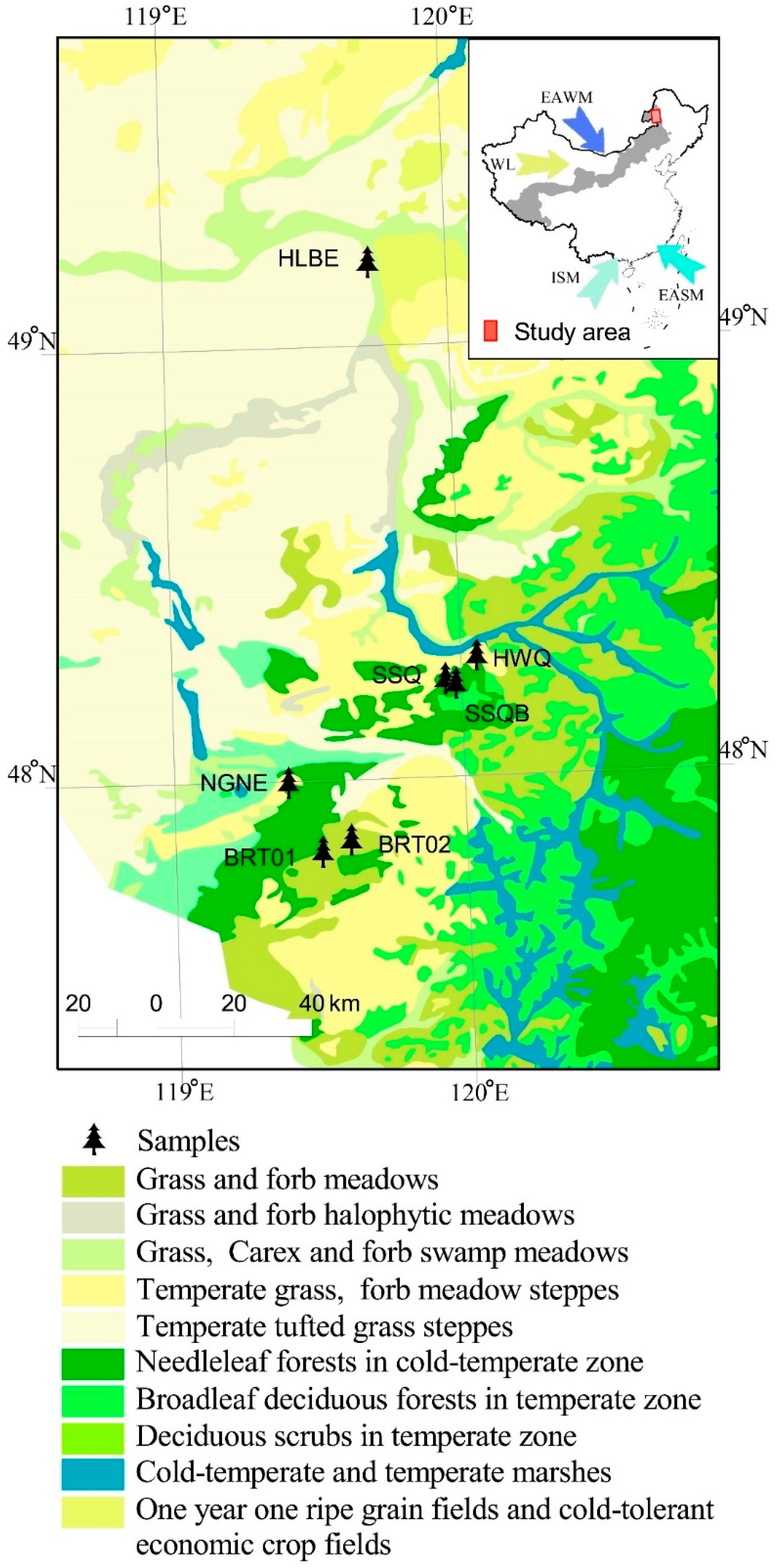
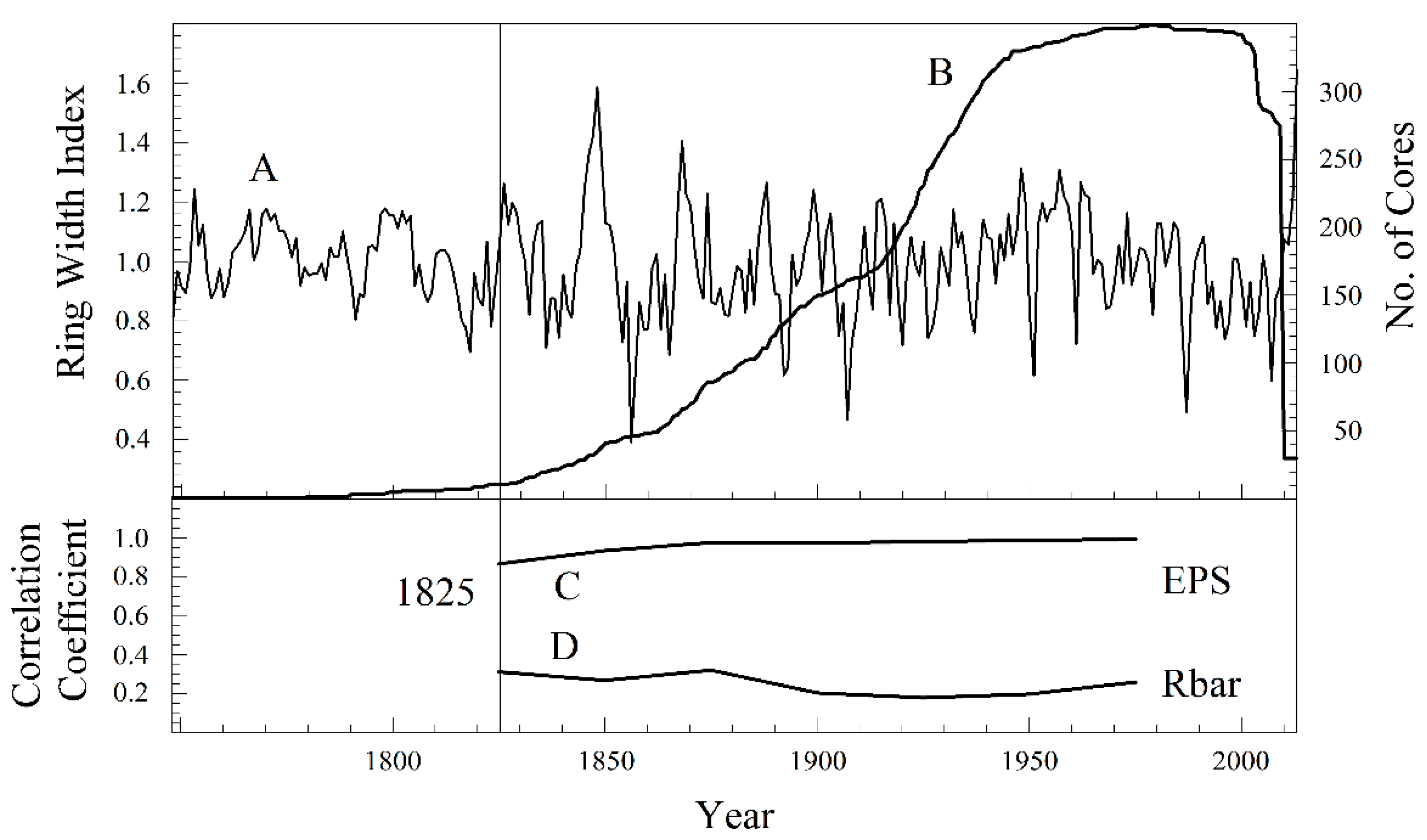
2.1. Tree-Ring Data and Ring-Width Chronology Development in the Central–Western Da Hinggan Mountains Region
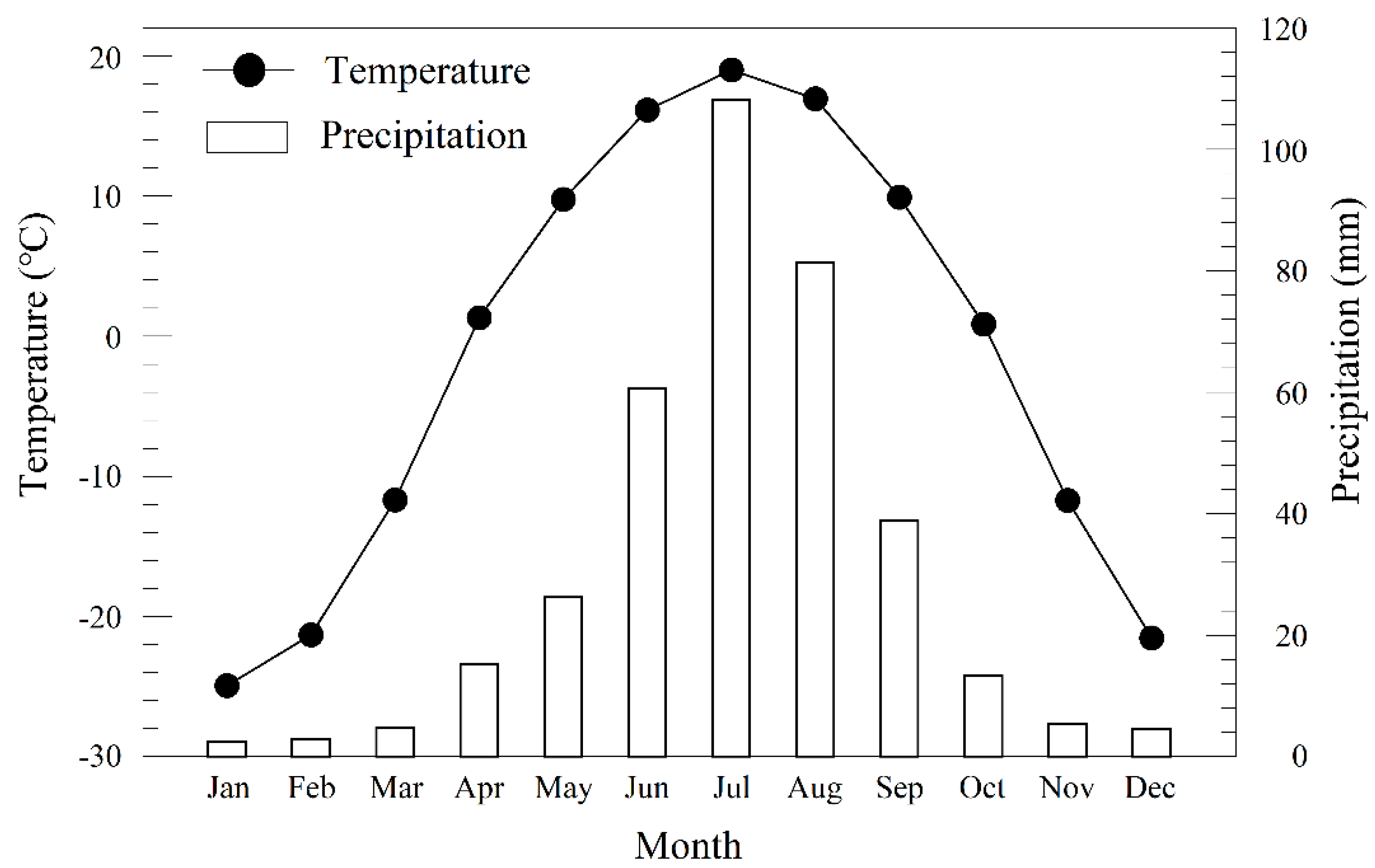
The CW–DHM, located in the transition zone between the arid area and the East Asian monsoon area, are very sensitive to climate change [13,18]. In total, 349 Mongolian pine (Pinus sylvestris var. mongolica Litv) cores from 7 locations (Figure 1) were used to establish a tree-ring width chronology in the CW–DHM region. Among these, 6 locations (HLBE, HWQ, SSQ, NGNE, BRT01, BRT02) have already been used to reconstruct the regional PDSI index [13]; this paper adds a new site, SSQB (Shenshuiquanbei).
All these individual cores were from the same tree species and the mean correlation between all individual series was very significant (r = 0.52, p < 0.001), therefore, we put all the individual ring-width series together [13] to generate a CW–DHM regionally representative chronology using the ARSTAN program [19]. During the chronology development process, we employed an exponential function or linear regression to remove the impacts of tree growth trends related to non-climatic factors and then synthesized these series into a chronology that represented regional variation with its variance stabilized with the Rbar-weighted method. Rbar was the mean correlation coefficient between all the possible pairs of ring-width series. Then, we acquired 3 types of chronologies using ARSTAN: standard (STD), residual (RES) and autoregressive (ARS) chronologies. Among these, the STD chronology preserved the low- and high-frequency signals. Thus, we employed the STD chronology in this paper (Figure 2), and it was named CW–DHM7 (Central-Western DaHinggan Mountains 7) for the period of 1748 to 2013 CE, spanning a total of 266 years. In this study, an expressed population signal (EPS) equal or greater than 0.85 was identified as a reliable threshold for constructing a credible chronology [20,21]. Thus, the receivable interval of our chronology was from 1825 to 2013 CE. The signal strength of our STD chronology was estimated using a moving Rbar and the EPS [21]. The statistical characteristics of the CW–DHM7 chronology were listed in Table 1.

2.2. Climatic Data

The climate parameters, including monthly precipitation (P) totals and mean monthly temperature (T), used in this paper, were acquired from the Climatic Research Unit time series (CRU TS4.01) [22] in 0.5° × 0.5° gridded datasets (47.5° N–49.5° N, 119.0° E–120.5° E, 1951–2013 CE) and monthly PDSI data from the CRU scPDSI 3.26e in 0.5° × 0.5° gridded datasets [23] (47.5° N–50.0° N, 117.5° E–122.5° E, 1982–2013 CE) were also used. In the CW–DHM region, high temperatures generally correspond to more precipitation, and the opposite is true as well. In this pattern, the precipitation and temperature vary at the same time, and both reach their peaks during the June–August period in a given year (Figure 3).

2.3. Remote Sensing Data

In this paper, we used a 15-day composite of the Advanced Very High Resolution Radiometer (AVHRR) Global Inventory Modeling and Mapping Studies (GIMMS) NDVI dataset, which had a resolution of 8 × 8 km, a range of 10 × 20 pixels and a coverage period from 1982 to 2013. The variation in NDVI ranged from −1 to 1, with values less than 0.1 corresponding to ice, inland water, desert and bare soil and values greater than 0.1 representing green vegetation coverage [24,25]. Here, the CNDVI data (119.34° E–120.07° E, 47.78° N–49.24° N, 1982–2013) from the GIMMS satellite datasets were our study target. We first extracted the maximum values from the whole time series data from each month (there were two periods of data each month, and we extracted the maximum value). Then, the NDVI values that were greater than 0.1 in the research area (10 × 20 pixel) were accumulated, thereby obtaining the CNDVI [26], from 1982 to 2013 month by month and year by year. The advantage of the CNDVI compared to the NDVI was that it prominently reflected the regional vegetation variation situation, especially in places where vegetation was inhomogeneously distributed or relatively sparse.

2.4. Statistic Method

To investigate the relationship among CW–DHM7, CNDVI and the climate parameters, we calculated the Pearson correlation coefficient (r). The analyses were based on monthly and seasonal (different combinations of consecutive months) climate data from the previous August to current July. In addition, partial correlations among CNDVI, temperature and precipitation were calculated. Because the data we gained from GIMMS satellite dataset only span 32 years (1982–2013 CE), we applied the bootstrap [27] and jackknife [28] methods to test the reliability and stability of the regression function during the calibration–verification period. The idea behind the bootstrap resampling technique is that the available observations of a variable contain the necessary information to construct an empirical probability distribution of any statistic of interest. The bootstrap method can provide standard errors of statistical estimators even when no theory exists. The jackknife technique is also known as the leave-one-out test. This technique was defined as the correlation of the time series after removing the values for one year progressively throughout the entire time period. In this study, the annual growth of climate factors in different time periods was calculated by slope analysis, and extremely high (low) CNDVI years were identified based on CNDVI values greater (less) than the mean plus one time the standard deviation (mean minus one time the standard deviation) of the reconstructed CNDVI series.
In addition, to investigate the influence of large-scale sea–atmospheric factors on the CNDVI variation, we calculated the correlations between the CNDVI and factors such as the global average temperature, Northern Hemisphere temperature [29], the Atlantic Multidecadal Oscillation (AMO) [30], the Summer North Atlantic Oscillation (SNAO) [31] and the Pacific Decadal Oscillation (PDO) [32]. The spatial correlation analysis was performed between our region CNDVI and the GIMMS CNDVI data using the Royal Netherlands Meteorological Institute Climate Explorer. The multi-taper method (MTM) program was used to perform the periodicity analysis for the reconstructed CNDVI sequence [33], and the program simulates the amplitude and phase evolution of a quasiperiodic signal over time.

3. Results

3.1. Variability Statistics of Regional Observed Meteorological Data

Since the CNDVI variation is tightly associated with climate factors, such as the moisture and temperature conditions [34], we investigated the changing trends of various climatic factors in the CW–DHM region during the periods 1951–1999 CE and 2000–2013 CE, according to observed meteorological records (Table 2). Some hydrological factors, such as precipitation [11], relative humidity [12] and PDSI [13], were already reconstructed on the basis of tree-ring width in the CW–DHM, and such analyses have shown that apparent abrupt changes from dry to wet conditions occurred in approximately 2000 CE. In addition, the global warming hiatus also occurred in approximately 2000 CE and the warming hiatus in northeastern China was more obvious [35]. During the periods 1951–1999 CE and 2000–2013 CE, the climatic conditions in the study area changed markedly both throughout the year and in the growing season. The climatic factors all improved to some extent during the period 2000–2013 CE, thereby favoring vegetation growth.

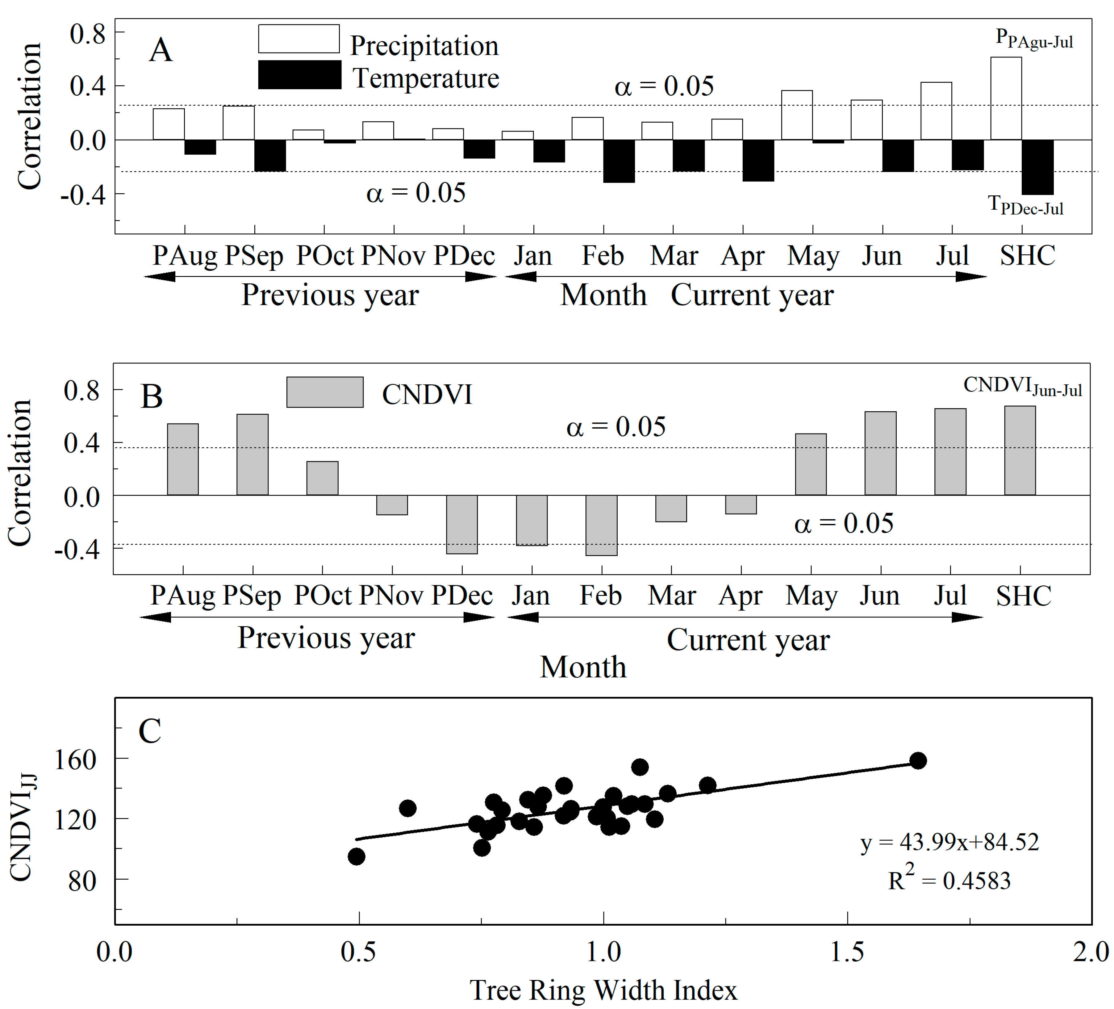
3.2. Correlation between CW–DHM7 and CNDVI

There was a significant positive correlation between the CW–DHM7 chronology and the CNDVI from June to July (CNDVIJJ), with r = 0.68 (p < 0.001, n = 32) (Figure 4A,B), the correlation can be seen clearly in the scatter diagram (Figure 4C). It should be noted that this correlation was improved by several extreme points. The situation that one point was deleted when building the relationship between tree-ring indices and climatic factors was common [36,37] and the deletion of several points will be debated as a regular scientific problem in dendroclimatology and dendroecology.
Partial correlation analysis (Table 3) showed that when precipitation was fixed, the correlation between the CNDVIJJ and the June–July mean temperature was 0.43 (n = 32, p < 0.017), while when the temperature was fixed, the correlation between the CNDVIJJ and the June to July precipitation was 0.47 (n = 32, p < 0.008).

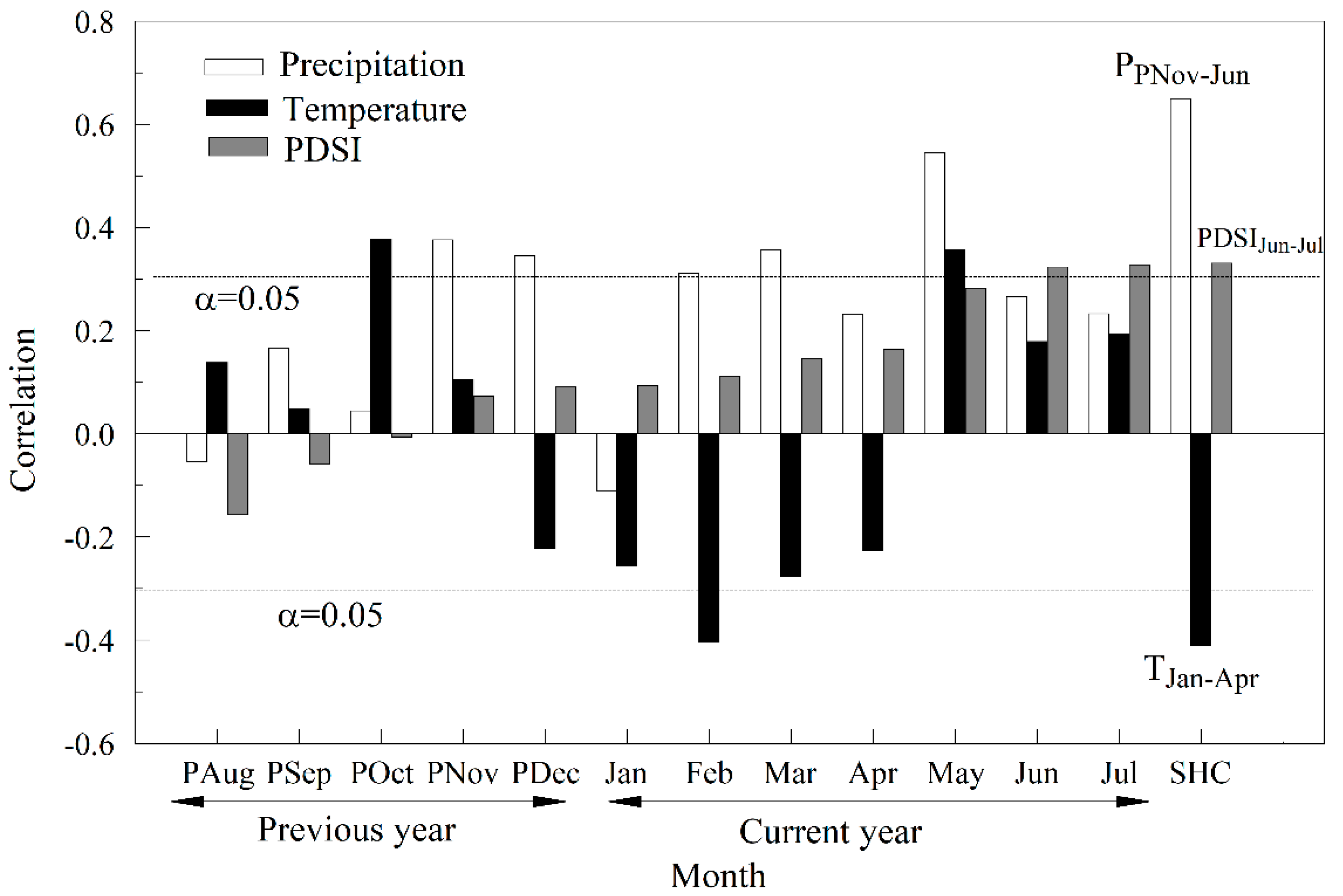
3.3. Correlations between CW–DHM Regional CNDVIJJ and Climate Parameters

The CNDVI reflects vegetation coverage variation in the CW–DHM region; however, the CNDVI is explicitly influenced by regional climate change. Indeed, the calculation of the response function shows that the CW–DHM regional CNDVIJJ is positively correlated with monthly average precipitation from September of the previous year to July of the current year, and the total precipitation from the previous November to the current June has the greatest impact, with r = 0.65 (p < 0.001, n = 32). The CNDVIJJ is negatively correlated with the mean temperature from December to April and from January to April. The CNDVIJJ is especially significantly correlated with temperature from January to April, with r = –0.41 (p < 0.019, n = 32). Obviously, the CNDVIJJ is affected by both temperature and precipitation. This finding is consistent with the PDSI, which is also influenced by both temperature and precipitation in the CW–DHM region [13]. Therefore, we calculated the correlation between the CNDVIJJ and the PDSI. We found that the CNDVIJJ is positively correlated with the PDSI values of each month from August of the previous year to June of the current year. After combining the months, the highest correlation between the CNDVIJJ and the PDSI was found to occur from May to June, with r = 0.61 (p < 0.001, n = 32) (Figure 5).

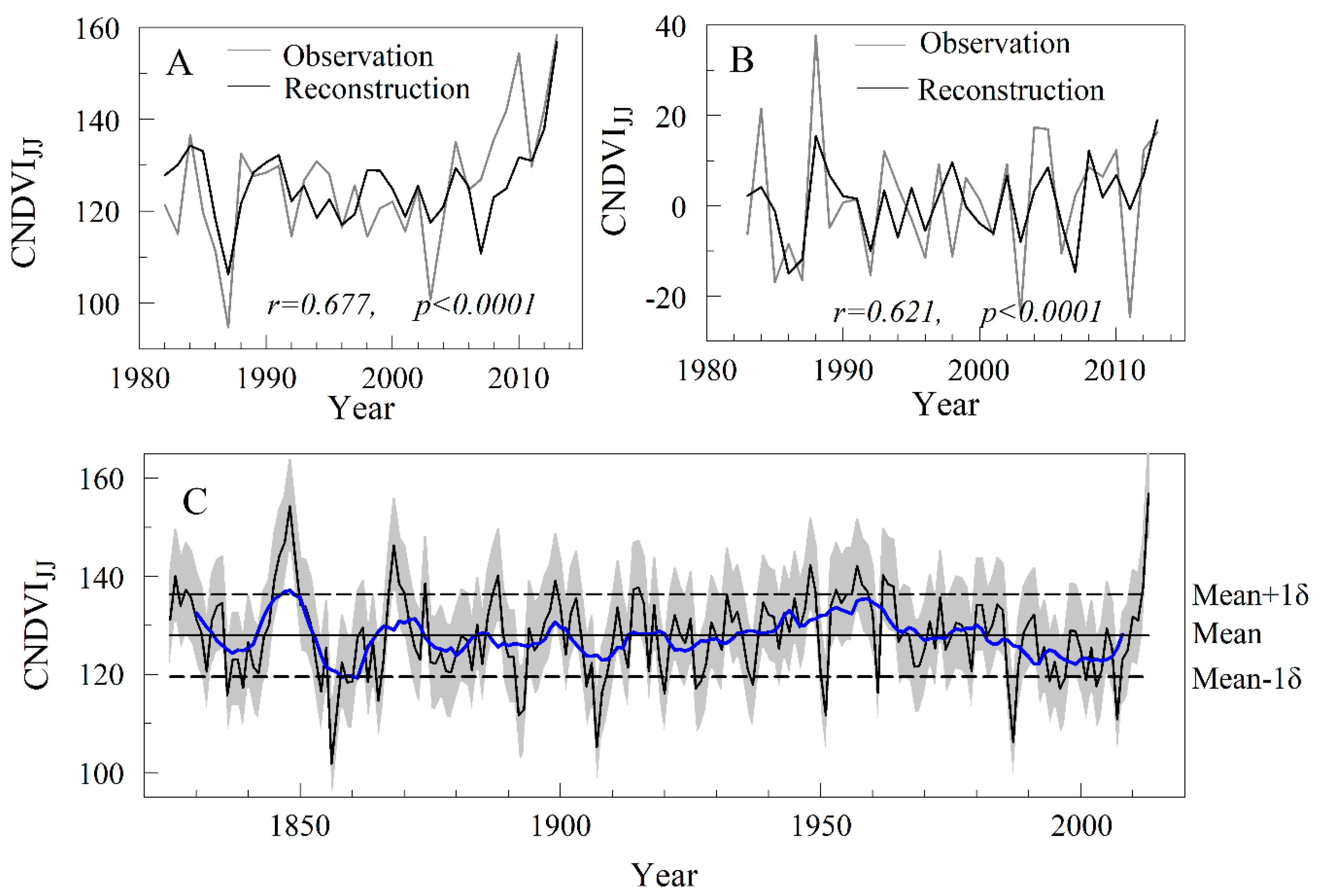
3.4. CNDVIJJ Reconstruction for the CW–DHM Region during the Period 1825–2013 CE

Based on the relationship between tree-ring width and CNDVIJJ during the period 1982–2013 CE, we designed the following transfer function to reconstruct the CNDVIJJ variation during the period 1825–2013 CE:
CNDVIJJ= 43.99 × STDt + 84.52
(n = 32, 1982–2013 CE, r = 0.68, p < 0.0001, R2 = 45.8%, R2adj = 44.0%, sd = 9.82, F = 25.39, D/W = 1.29)
Where STDt is the CW–DHM chronology value in year t, the explained variance is 45.8% (44.0% after the adjustment for the loss of the degree of freedom), and the Durbin–Watson value (D/W) [38] is 1.29. The Durbin–Watson value is used to test whether there is autocorrelation within the series; when n = 32, a D/W value between 1.28 and 2.72 indicates that there is no autocorrelation within the series. The D/W value of 1.29 in this paper indicates slight autocorrelation. Additionally, the correlation after the first-order difference of the observed and reconstructed series is 0.62 (n = 32, p < 0.001). Our reconstruction tracked the changes characteristic of the observed CNDVIJJ at both high and low frequencies (Figure 6).
With the software MATLAB R2015b, the bootstrap and jackknife methods were used to verify our reconstruction model. The results demonstrated that the r, R2, R2adj, F, p and D/W values calculated by the bootstrap and jackknife methods are close to those of the original dataset, indicating that the regression model is quite reliable and stable (Table 4).
According to Equation (1), we reconstructed the CNDVIJJ variation history in the CW–DHM region during the period 1825–2013 CE. The average value of CNDVIJJ from 1825 to 2013 CE was 127.94, and the standard deviation (1σ) was ±8.41. Therefore, the values greater than 136.35 (mean + 1σ) in the reconstructed series were extremely high CNDVIJJ years, the values less than 119.53 (mean–1σ) were extremely low CNDVIJJ years, and the values between 119.53 and 136.35 were the normal years. Thus, in the entire reconstructed series, high and low CNDVIJJ values each occur in 28 years, each accounting for 14.81% of the total. The proportion of extremely low CNDVIJJ years is equivalent to the proportion of extremely high CNDVIJJ years. The top ten high and low CNDVIJJ values are listed in Table 5.

3.5. The Spatial Representation of CNDVIJJ in the CW–DHM Region

The spatial correlation results indicate that the CNDVIJJ in the CW–DHM, based on both the observed and reconstructed series from 1982 to 2013 CE, has good spatial representativeness and consistency in terms of larger regional vegetation change responses (Figure 7).

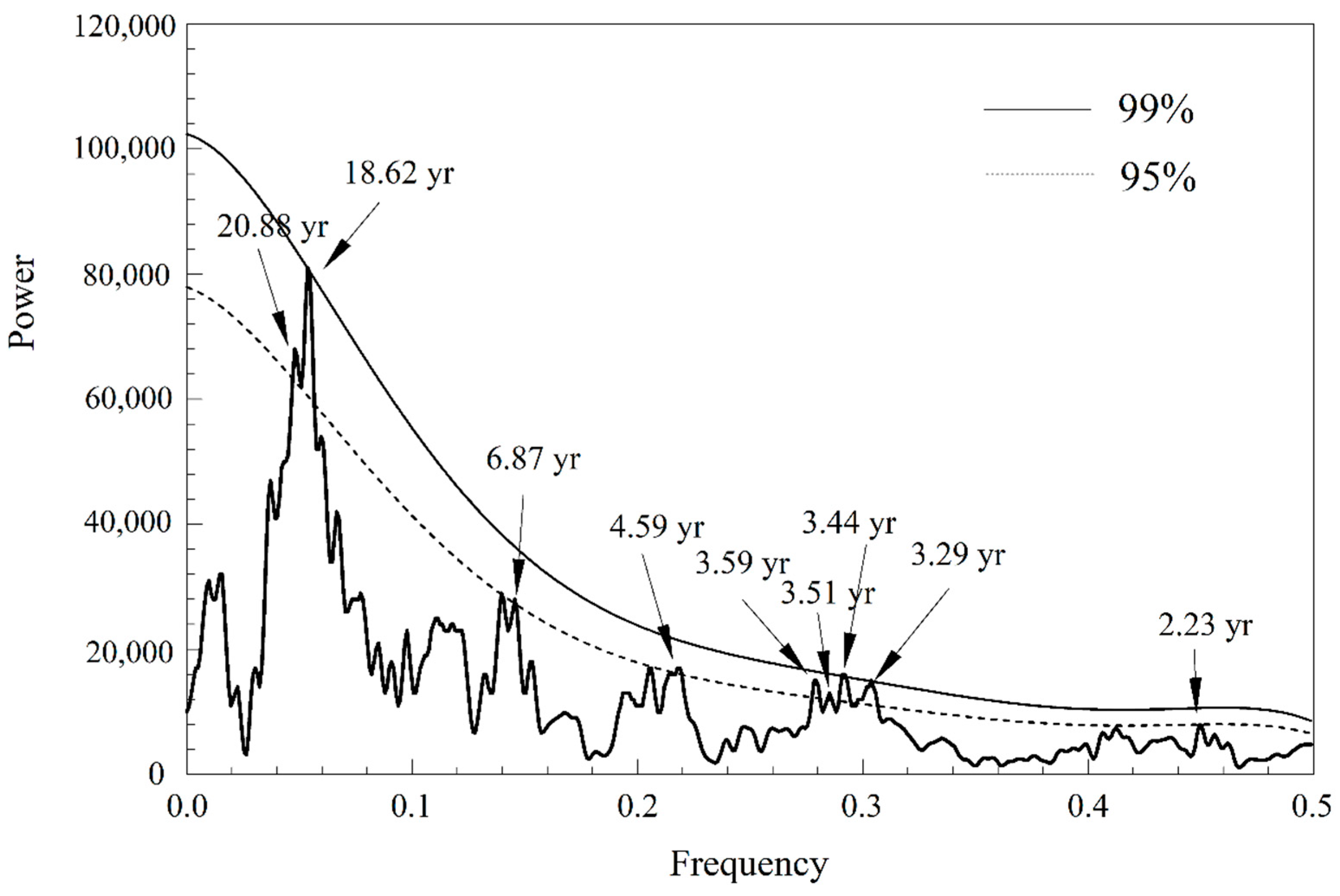
3.6. Periodicity Analysis of CNDVIJJ Variation over the Past 189 Years

The MTM results show that the CNDVIJJ in the CW–DHM region over the past 189 years had a number of significant cycles, such as 3.44 and 3.29 y quasi-cycles at the 99% confidence level, and 20.88, 18.62, 6.87, 4.59, 3.59, 3.51 and 2.23 y quasi-cycles at the 95% confidence level (Figure 8).

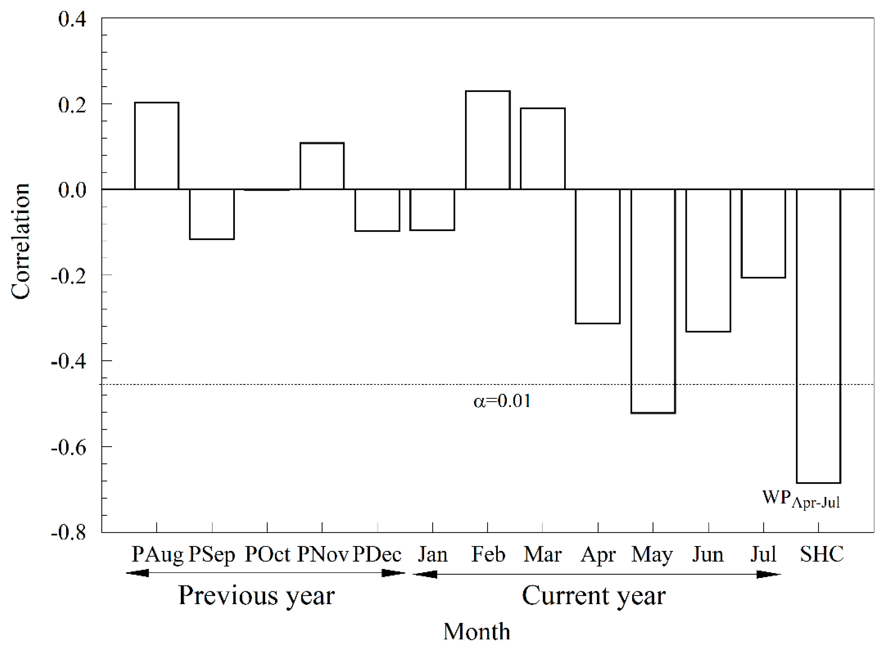
3.7. The Connections between CW–DHM Regional CNDVIJJ Variation and Large-Scale Sea–Atmospheric Factors

The results of correlations between the CNDVIJJ and large-scale sea–atmospheric factors show that the CNDVIJJ is significantly correlated with these sea–atmospheric parameters (Table 6). Notably, the correlation between the CNDVIJJ and the western Pacific patterns is high, with r = –0.69 (p < 0.001, Figure 9). The teleconnection patterns influence the vegetation variation through the influence of the sea surface temperature in the western Pacific region on the large-scale regional atmospheric circulation, which in turn influences the regional temperature and precipitation.

4. Discussion

4.1. The Relationship between the CNDVI Changes and Tree-Ring Chronology in CW–DHM Region

Previous studies show that the CNDVI is tightly associated with climatic factors, such as the hydrologic and temperature conditions [35]. In the CW–DHM, the vegetation density (CNDVI) is greatly influenced by the combined effects of temperature and precipitation. In addition, tree-ring width was significantly affected by similar climate limiting factors [13]. CNDVI is an index generated by the reflection of plant leaves on the red and near-infrared light bands, which mainly reflect the greenness of plant leaves. The index is also strongly related to the photosynthetic activity of vegetation [39]. The width of the tree rings indicates the radial growth of the tree, and its growth rate is mainly determined by the net accumulation of photosynthesis and respiration. Chlorophyll is essential for plant photosynthesis, and its amount will determine the photosynthesis accumulation in plants, which in turn affects the radial growth of plants. When the limiting factor functions on the vegetation, it will inhibit the photosynthesis of plant leaves, which slow the radial growth of the plants, and control the tree ring width and CNDVI [40]. Moreover, trees are important forms of vegetation and their own growth statuses represent a partial change in vegetation coverage. Therefore, tree-ring chronologies reflect the summer CNDVI changes.

4.2. The Spatial and Temporal Variations in Vegetation during the Last 189 Years in the CW–DHM Region

China is strongly influenced by the East Asian Summer Monsoon (EASM), especially monsoon-related precipitation. During the summer monsoon season, the EASM brings a large amount of water moisture from the Pacific Ocean to the inland of China. The stronger the monsoon is, the greater the amount of moisture delivered to the interior. During the northward progression of the EASM, the Da Hinggan Mountains hinder the northward movement of the EASM.
In our study area, precipitation and temperature in June and July have basically the same effect on vegetation coverage, although the precipitation effect is slightly stronger. That is, the dry and wet conditions in June and July, which are related to the strength of the EASM, seriously affect the vegetation coverage. Consequently, it is easy to understand why a weak EASM caused a well-known severe drought during the late 1920s in northern China (1926–1931 CE) [41,42,43,44,45]. Our reconstructed CNDVIJJ data show low values, and the vegetation coverage was significantly reduced at that time. Similarly, from 1876 to 1878 CE, 13 provinces in northern China suffered from a severe drought named the “Ding–Wu severe drought” [46,47,48], and the serious reduction in vegetation cover caused by this drought was also observed in our reconstructed series (Figure 6).
On the other hand, an intense EASM brings abundant precipitation, which is beneficial to enhanced vegetation coverage. An intense EASM led to a nationwide flooding disaster in 1954 [49], and high values are present at this time in our reconstructed CNDVIJJ series. After 2000 CE, the EASM continued to strengthen, leading to increased precipitation in the study area [13], which further increased the CNDVIJJ in the the CW–DHM region.
In our 189 year reconstructed CNDVIJJ series, there are 28 extremely high years and 28 extremely low years, each accounting for 14.8% of the total sequence, with equal proportions. The periods with high canopy greenness are 1830–1833 CE, 1842–1852 CE, 1865–1873 CE, 1884–1886 CE, 1898–1901 CE, 1913–1920 CE, 1934–1968 CE, 1975–1981 CE and after 2003 CE, and the periods with low canopy greenness are 1834–1841 CE, 1853–1864 CE, 1874–1883 CE, 1887–1897 CE, 1902–1912 CE, 1921–1933 CE, 1969–1974 CE and 1982–2007 CE.
The vegetation coverage, as represented by CNDVIJJ, clearly decreased in the CW–DHM from 1950 to 2000 CE (Figure 6). At the same time, the PDSI index in the area also decreased [13], and the climate exhibited drier conditions. Therefore, the observed and reconstructed CNDVIJJ datasets exhibited consistent variation trends from 1982 to 2003 CE (Figure 6A,B).
The meteorological conditions improved after 2000 CE (Table 2), and the vegetation coverage increased significantly in our CNDVIJJ reconstruction. This trend not only appears spontaneously with the regional PDSI index [13] but also coincides with the results of the large-scale vegetation coverage increase obtained by previous research [50]. This illustrated that our reconstructed results can effectively reflect large-scale vegetation coverage variation history in the past 189 years.
From the spatial correlation analysis, we found that the vegetation variation situation in the CW–DHM region reflects a cosmopolitan phenomenon (Figure 7). The global green land increased by 5% according to the analysis of satellite-derived global remote sensing data from 2000 to 2017 CE, particularly in China [51]. This finding is in line with the timing and the process of vegetation enhancement we observed in the CW–DHM region (Figure 7). Furthermore, this finding is in accordance with our current investigation that demonstrated that vegetation has increased during the last two decades in some parts of the world [50,51].
Spatial correlation analysis results also reveal that our study area is positively correlated with southern Central Siberia, eastern Mongolia and northeastern and eastern China. These results illustrate that the CNDVI values in these areas also decreased from 1982 to 2003 CE and increased from 2003 to 2013 CE. Our reconstruction captured this phenomenon very well (Figure 7), and the spatial correlations between the observations and the reconstructions are very good. Therefore, we thought that the changes of vegetation coverage in these regions might reflect their common response to climate changes. In other words, climate variability is, at least at present, beneficial to increasing vegetation coverage in these areas.

4.3. Possible Mechanism of CNDVIJJ Variation in the CW–DHM Region

Precipitation and temperature are the fundamental elements that influence vegetation coverage. Climate change in the CW–DHM region is also affected by large-scale sea–atmosphere coupling. For example, the climate variation in the CW–DHM region is tightly associated with the AMO, SNAO, and PDO [13]. However, these climate factors do not directly affect CNDVIJJ variation in the CW–DHM region; instead, these large-scale climate factors first generate regional climate changes, and then regional climate factors create CNDVIJJ changes. Therefore, it is not surprising that the CNDVIJJ in the CW–DHM region is significantly correlated with AMO, SNAO and PDO. (Table 6). Notably, the correlation coefficient between CNDVIJJ and teleconnection patterns in the western Pacific region reaches –0.69 (p < 0.001, April–July, n = 32, Figure 9), indicating that the western Pacific region has a very strong influence on the climate of the CW–DHM and CNDVIJJ.
Affected by the periodic climate variation in the study region [10,52,53], the CNDVIJJ undoubtedly exhibits periodic changes. The cycles we detected, such as the 18.62 and 20.88 y quasi-cycles, correspond to two cycles of sunspot activity (~22 y) [54]. Hence, there is an influence of sunspot activity on climate and the CNDVIJJ. Additionally, the 3.29 to 6.87 y quasi-cycles correspond to the El Niño-Southern Oscillation (ENSO) activity period [55]. The correlation between our CNDVIJJ dataset and ENSO in the Niño 4 area in the current July reaches –0.24 (p < 0.2), highlighting the influence that ENSO activity imposes on the CNDVIJJ in the study region. The 2.23 y quasi-cycle corresponds to the extensively documented tropospheric biennial oscillation (TBO) [56].
These calculation results clearly show that solar activity, surface temperature in the Northern Hemisphere and sea–atmosphere coupling across large areas in all hemispheres play some role in the climate change in the CW–DHM in multiple ways and thus influence the CNDVIJJ variation in the CW–DHM area. In addition, these drivers not only affect the change in the vegetation coverage variation in the CW–DHM but also affect the NDVI changes in its adjacent regions as well, making the changes in the CNDVIJJ in the CW–DHM area comparable to larger regional CNDVI fluctuations (Figure 7).

5. Conclusions

In this paper, we obtained a CNDVI sequence using 32 y NDVI data recorded by existing satellite observations, combined with tree-ring width data from the CW–DHM region. We found that the chronology in the CW–DHM was significantly correlated with the June–July CNDVI, with an explained variance of 45.8% (r = 0.68, n = 32, p < 0.0001) and an explained variance of 44.0% after the adjustment for the loss of the degree of freedom. On this basis, we designed a transfer function to reconstruct the vegetation changes in the CW–DHM region over the past 189 years. The CW–DHM regional greenness change was closely related to the local climate conditions. Less precipitation and drier climate conditions resulted in sparser vegetation. After the year 2000, the CNDVIJJ in the CW–DHM region showed high values, indicating that the dense vegetation was consistent with the increase in vegetation growth in some parts of Asia at the same time. Therefore, excellent spatial and temporal consistency existed between the vegetation change in the CW–DHM and the vegetation change in the southern Central Siberia, eastern Mongolia and northeastern and eastern China, which was also confirmed by the results of spatial correlation analysis. Interestingly, the CNDVIJJ variation in the CW–DHM area was significantly influenced by climate change; therefore, factors affecting regional climate change, such as sunspot activity and large-scale ocean–atmosphere coupling factors, such as AMO, SNAO, PDO and ENSO, are transmitted through climate change, further influencing the fluctuations in vegetation density in the study region. These ocean–atmosphere coupling factors not only affect the climate–vegetation coverage variation in the CW–DHM region but also affect the NDVI changes in its adjacent regions simultaneously. Thus, it is not difficult to understand why the CW–DHM regional vegetation variation is significantly connected with these regions in Asia. This study is of great significance for improving our understanding of the process of vegetation change and the local ecological situation in the CW–DHM region.

Author Contributions

data curation: R.L. and Y.S.; formal analysis, R.L. and C.S.; funding acquisition, Y.L.; investigation, R.L., X.L., H.S., Q.L., Q.C., M.R. and L.W.; methodology, R.L. and Y.L.; software, R.L. and Y.S.; visualization, R.L. and Y.S.; writing—original draft, R.L.; writing—review and editing, R.L. and Y.L. Authorship must be limited to those who have contributed substantially to the work reported. All authors have read and agreed to the published version of the manuscript.

Funding

This work was supported by the CAS Research Program (QYZDJ–SSW–DQC021, XDB40000000); the National Natural Science Foundation of China (NSFC 41630531, 41873021); Youth Innovation Promotion Association of CAS (No. 2017451); West Light Foundation of CAS, the Key Project of IEECAS; and the State Key Laboratory of Loess and Quaternary Geology, Institute of Earth Environment, CAS (SKLLQG1916).

Institutional Review Board Statement

Not applicable.

Informed Consent Statement

Not applicable.

Conflicts of Interest

The authors declare no conflict of interest.

References

  1. Hu, C.J.; Fu, B.J.; Liu, G.H.; Jin, T.T.; Guo, L. Vegetation patterns influence on soil microbial biomass and functional diversity in a hilly area of the Loess Plateau, China. J. Soils Sediment. 2010, 10, 1082–1091. [Google Scholar] [CrossRef]
  2. Piao, S.L.; Fang, J.Y.; He, J.S. Variations in vegetation net primary production in the Qinghai–Xizang Plateau, China, from 1982 to 1999. Clim. Chang. 2006, 74, 253–267. [Google Scholar] [CrossRef]
  3. Zhao, Y.S. Principle and Method of Remote Sensing Applied Analysis; Science Press: Beijing, China, 2003. [Google Scholar]
  4. D’Arrigo, R.D.; Malmstrom, C.M.; Jacoby, G.C.; Los, S.O.; Bunker, D.E. Correlation between maximum latewood density of annual tree rings and NDVI based estimates of forest productivity. Int. J. Remote Sens. 2000, 21, 2329–2336. [Google Scholar] [CrossRef]
  5. Gazol, A.; Camarero, J.J.; Vicente-Serrano, S.M.; Sanchez-Salguero, R.; Gutierrez, E.; de Luis, M.; Sanguesa-Barreda, G.; Novak, K.; Rozas, V.; Tiscar, P.A.; et al. Forest resilience to drought varies across biomes. Glob. Chang. Biol. 2018, 24, 2143. [Google Scholar] [CrossRef] [PubMed]
  6. Kaufmann, R.K.; D’Arrigo, R.D.; Paletta, L.F.; Tian, H.Q.; Jolly, W.M.; Myneni, R.B. Identifying climatic controls on ring width: The timing of correlations between tree rings and NDVI. Earth Interact. 2008, 12, 1–14. [Google Scholar] [CrossRef] [Green Version]
  7. Sankey, T.T. Decadal–scale aspen changes: Evidence in remote sensing and tree ring data. Appl. Veg. Sci. 2012, 15, 84–98. [Google Scholar] [CrossRef]
  8. Xu, P.P.; Zhou, T.; Yi, C.X.; Fang, W.; Hendrey, G.; Zhao, X. Forest drought resistance distinguished by canopy height. Environ. Res. Lett. 2018, 13, 075003. [Google Scholar] [CrossRef] [Green Version]
  9. Leavitt, S.W.; Chase, T.N.; Rajagopalan, B.; Lee, E.; Lawrence, P.J. Southwestern U.S. tree-ring carbon isotope indices as a possible proxy for reconstruction of greenness of vegetation. Geophys. Res. Lett. 2008, 35, L12704. [Google Scholar] [CrossRef]
  10. Gao, J.X.; Shi, Z.J.; Xu, L.H.; Yang, X.H.; Jia, Z.Q.; Lü, S.H.; Feng, C.Y.; Shang, J.X. Precipitation variability in Hulunbuir, Northeastern China since 1829 AD reconstructed from tree-rings and its linkage with remote oceans. J. Arid Environ. 2013, 95, 14–21. [Google Scholar] [CrossRef]
  11. Liu, Y.; Bao, G.; Song, H.M.; Cai, Q.F.; Sun, J.Y. Precipitation reconstruction from Hailar pine (Pinus sylvestris var mongolica) tree rings in the Hailar region Inner Mongolia China back to 1865 AD. Palaeogeogr. Palaeoclimatol. Palaeoecol. 2009, 282, 81–87. [Google Scholar] [CrossRef]
  12. Sun, B.; Liu, Y.; Lei, Y. Growing season relative humidity variations and possible impacts on Hulunbuir grassland. Sci. Bull. 2016, 61, 728–736. [Google Scholar] [CrossRef] [Green Version]
  13. Liu, R.S.; Liu, Y.; Li, Q.; Song, H.M.; Li, X.X.; Sun, C.F.; Cai, Q.F.; Song, Y. Seasonal Palmer Drought Severity Index reconstruction using tree–ring widths from multiple sites over the central–western Da Hinggan Mountains, China since 1825 AD. Clim. Dyn. 2019, 53, 3661–3674. [Google Scholar] [CrossRef]
  14. Chen, Z.J.; Li, J.B.; Fang, K.Y.; Davi, N.K.; He, X.Y.; Cui, M.X.; Zhang, X.L.; Peng, J.J. Seasonal dynamics of vegetation over the past 100 years inferred from tree rings and climate in Hulunbei’er steppe, northern China. J. Arid Environ. 2012, 83, 86–93. [Google Scholar] [CrossRef] [Green Version]
  15. Liang, E.Y.; Eckstein, D.; Liu, H.Y. Assessing the recent grassland greening trend in a long–term context based on tree–ring analysis: A case study in north China. Ecol. Indic. 2009, 9, 1280–1283. [Google Scholar] [CrossRef]
  16. Yao, J.; He, X.Y.; Li, X.Y.; Chen, W. Monitoring responses of forest to climate variations by MODIS NDVI: A case study of Hun river upstream, northeastern China. Eur. J. For. Res. 2012, 131, 705–716. [Google Scholar] [CrossRef]
  17. Sun, C.F.; Liu, Y.; Song, H.M.; Li, Q.; Cai, Q.F.; Wang, L.; Fang, C.X.; Liu, R.S. Tree-ring evidence of the impacts of climate change and agricultural cultivation on vegetation coverage in the upper reaches of the Weihe River, northwest China. Sci. Total Environ. 2020, 707, 136160. [Google Scholar] [CrossRef]
  18. Gao, Z.T.; Hu, Z.Z.; Jha, B.; Yang, S.; Zhu, J.S.; Shen, B.Z.; Zhang, R.J. Variability and predictability of northeast China climate during 1948–2012. Clim. Dyn. 2014, 43, 787–804. [Google Scholar] [CrossRef]
  19. Cook, E.R. A Time Series Analysis Approach to Tree–ring Standardization. Ph.D. Thesis, University of Arizona, Tucson, AZ, USA, 1985. [Google Scholar]
  20. Cook, E.R.; Kairiukstis, L.A. Methods of Dendrochronology; Kluwer Academic Publishers: Dordrecht, The Netherlands, 1990. [Google Scholar]
  21. Wigley, T.M.L.; Briffa, K.R.; Jones, P.D. On the average value of correlation time series, with applications in dendroclimatology and hydrometeorology. J. Clim. Appl. Meteor. 1984, 23, 201–213. [Google Scholar] [CrossRef]
  22. Mitchell, T.D.; Jones, P.D. An improved method of constructing a database of monthly climate observations and associated high resolution grids. Int. J. Climatol. 2005, 25, 639–712. [Google Scholar] [CrossRef]
  23. Van der Schrier, G.; Barichivich, J.; Briffa, K.R.; Jones, P.D. A scPDSI-based global data set of dry and wet spells for 1901–2009. J. Geophys. Res. Atmos. 2013, 118, 4025–4048. [Google Scholar] [CrossRef]
  24. Song, Y.; Ma, M.; Veroustraete, F. Comparison and conversion of AVHRR GIMMS and SPOT VEGETATION NDVI data in China. Int. J. Remote Sens. 2010, 31, 2377–2392. [Google Scholar] [CrossRef]
  25. Tucker, C.J.; Sellers, P.J. Satellite remote sensing of primary production. Int. J. Remote Sens. 1986, 7, 1395–1416. [Google Scholar] [CrossRef]
  26. Song, Y.; Jin, L.; Wang, H.B. Vegetation changes along the Qinghai–Tibet Plateau engineering corridor since 2000 induced by climate Change and Human Activities. Remote Sens. 2018, 10, 95. [Google Scholar] [CrossRef] [Green Version]
  27. Efron, B. Bootstrap methods: Another look at the jackknife. Ann. Stat. 1979, 7, 1–26. [Google Scholar] [CrossRef]
  28. Mosteller, F.; Tukey, J.W. Data Analysis and Regression: A Second Course in Statistics; Addison–Wesley Series in Behavioral Science; Addison Wesley Publishing Company: Reading, PA, USA, 1977; pp. 1–588. [Google Scholar]
  29. Morice, C.P.; Kennedy, J.J.; Rayner, N.A.; Jones, P.D. Quantifying uncertainties in global and regional temperature change using an ensemble of observational estimates: The HadCRUT4 data set. J. Geophys. Res. Atmos. 2012, 117, D08101. [Google Scholar] [CrossRef]
  30. Van Oldenborgh, G.J.; Te Raa, L.A.; Dijkstra, H.A.; Philip, S.Y. Frequency- or amplitude-dependent effects of the Atlantic meridional overturning on the tropical Pacific Ocean. Ocean Sci. 2009, 5, 293–301. [Google Scholar] [CrossRef] [Green Version]
  31. Folland, C.K.; Knight, J.; Linderholm, H.W.; Fereday, D.; Ineson, S.; Hurrell, J.W. The Summer North Atlantic oscillation: Past, present, and future. J. Clim. 2009, 22, 1082–1103. [Google Scholar] [CrossRef]
  32. Mantua, N.J.; Hare, S.R. The Pacific Decadal Oscillation. J. Oceanogr. 2002, 58, 35–44. [Google Scholar] [CrossRef]
  33. Thomson, D.J. Spectrum estimation and harmonic-analysis. Proc. IEEE 1982, 70, 1055–1096. [Google Scholar] [CrossRef] [Green Version]
  34. Carlson, T.N.; Gillies, R.R.; Perry, E.M. A method to make use of thermal infrared temperature and NDVI measurements to infer surface soil water content and fractional vegetation cover. Remote Sens. Rev. 1994, 9, 161–173. [Google Scholar] [CrossRef]
  35. Du, Q.; Zhang, M.; Wang, S.; Che, C.; Ma, R.; Ma, Z. Changes in air temperature of China in response to global warming hiatus. Acta Geogr. Sin. 2018, 73, 1748–1764. [Google Scholar]
  36. Liu, Y.; Wang, Y.C.; Li, Q.; Song, H.; Zhang, Y.H.; Yuan, Z.L.; Wang, Z.Y. Tree-ring stable carbon isotope-based May–July temperature reconstruction over Nanwutai, China, for the past century and its record of 20th century warming. Quat. Sci. Rev. 2014, 93, 67–76. [Google Scholar] [CrossRef]
  37. Liu, Y.; Wang, Y.C.; Li, Q.; Song, H.; Linderhlom, H.M.; Leavitt, S.W.; Wang, R.Y.; An, Z.S. Reconstructed May–July mean maximum temperature since 1745 AD based on tree-ring width of Pinus tabulaeformis in Qianshan Mountain, China. Palaeogeogr. Palaeoclimatol. Palaeoecol. 2013, 388, 145–152. [Google Scholar] [CrossRef]
  38. Durbin, J.; Watson, G.S. Testing for serial correlation in least squares regression I. Biometrika 1950, 37, 409–428. [Google Scholar]
  39. Wang, J.; Rich, P.M.; Price, K.P.; Kettle, W.D. Relations between NDVI and tree productivity in the central Great Plains. Int. J. Remote Sens. 2004, 25, 3127–3138. [Google Scholar] [CrossRef]
  40. Wang, W.Z.; Liu, X.H.; Chen, T.; An, W.L.; Xu, G.B. Reconstruction of regional NDVI using tree-ring width chronologies in the Qilian Mountains, northwestern China. Chin. J. Plant Ecol. 2010, 34, 1033–1044. [Google Scholar]
  41. Liang, E.Y.; Liu, X.H.; Yuan, Y.J.; Qin, N.S.; Fang, X.Q.; Huang, L.; Zhu, H.F.; Wang, L.L.; Shao, X.M. The 1920s drought recorded by tree rings and historical documents in the semi-arid and arid areas of northern China. Clim. Chang. 2006, 79, 403–432. [Google Scholar] [CrossRef]
  42. Liu, X.H.; Zhang, X.W.; Zhao, L.J.; Xu, G.B.; Wang, L.X.; Sun, W.Z.; Zhang, Q.L.; Wang, W.Z.; Zeng, X.M.; Wu, G.J. Tree ring δ18o reveals no long–term change of atmospheric water demand since 1800 in the northern Great Hinggan Mountains, China. J. Geophys. Res. Atmos. 2017, 122, 6697–6712. [Google Scholar] [CrossRef] [Green Version]
  43. Liu, Y.; Lei, Y.; Sun, B.; Song, H.M.; Li, Q. Annual precipitation variability inferred from tree–ring width chronologies in the Changling–Shoulu region, China, during AD 1853–2007. Dendrochronologia 2013, 31, 290–296. [Google Scholar] [CrossRef]
  44. Liu, Y.; Lei, Y.; Sun, B.; Song, H.M.; Sun, J.Y. Annual precipitation in Liancheng, China, since 1777 AD derived from tree rings of Chinese pine (pinus tabulaeformis carr.). Int. J. Biometeorol. 2013, 57, 927–934. [Google Scholar] [CrossRef]
  45. Liu, Y.; Sun, B.; Song, H.M.; Lei, Y.; Wang, C.Y. Tree–ring–based precipitation reconstruction for Mt. Xinglong, China, since AD 1679. Quat. Int. 2013, 283, 46–54. [Google Scholar] [CrossRef]
  46. Hao, Z.X.; Zheng, J.Y.; Wu, G.F.; Zhang, X.Z.; Ge, Q.S. 1876–1878 severe drought in North China: Facts, impacts and climatic background. Chin. Sci. Bull. 2010, 55, 3001–3007. [Google Scholar] [CrossRef]
  47. Kang, S.Y.; Yang, B.; Qin, C.; Wang, J.L.; Shi, F.; Liu, J.J. Extreme drought events in the years 1877–1878, and 1928, in the southeast Qilian Mountains and the air–sea coupling system. Quat. Int. 2013, 283, 85–92. [Google Scholar] [CrossRef]
  48. Zhang, D.E.; Liang, Y.Y. A long lasting and extensive drought event over China during1876–1878. Adv. Clim. Chang. Res. 2010, 6, 106–112. (in Chinese). [Google Scholar]
  49. Cheng, M.D. Perspective on Major Emergencies in Contemporary China; Chinese Communist Party History Publishing House: Beijing, China, 2008. [Google Scholar]
  50. Piao, S.L.; Wang, X.H.; Ciais, P.; Zhu, B.; Wang, T.; Liu, J. Changes in satellite–derived vegetation growth trend in temperate and boreal Eurasia from 1982 to 2006. Glob. Chang. Biol. 2011, 17, 3228–3239. [Google Scholar] [CrossRef]
  51. Chen, C.; Park, T.; Wang, X.; Piao, S.; Xu, B.; Chaturvedi, R.K.; Fuchs, R.; Brovkin, V.; Ciais, P.; Fensholt, R.; et al. China and India lead in greening of the world through land-use management. Nat. Sustain. 2019, 2, 122–129. [Google Scholar] [CrossRef]
  52. Yu, J.; Zhou, G.; Liu, Q.J. Tree–ring based summer temperature regime reconstruction in Xiaoxing Anling Mountains, northeastern China since 1772 CE. Palaeogeogr. Palaeoclimatol. Palaeoecol. 2017, 495, 13–23. [Google Scholar] [CrossRef]
  53. Wang, Y.C.; Liu, Y. Reconstruction of March–June precipitation from tree rings in central Liaoning, China. Clim. Dyn. 2016, 49, 1–11. [Google Scholar] [CrossRef]
  54. Han, Y.B.; Han, Y.G. Wavelet analysis of sunspot relative numbers. Chin. Sci. Bull. 2002, 47, 609–612. [Google Scholar] [CrossRef]
  55. Kaplan, A.; Cane, M.A.; Kushnir, Y.; Clement, A.C.; Blumenthal, M.B.; Rajagopalan, B. Analyses of global sea surface temperature 1856–1991. J. Geophys. Res. 1998, 103, 18567–18589. [Google Scholar] [CrossRef] [Green Version]
  56. Meehl, G.A.; Arblaster, J.M. The Tropospheric Biennial Oscillation and Indian Monsoon rainfall. Geophys. Res. Lett. 2002, 28, 1731–1734. [Google Scholar] [CrossRef]
Figure 1. The locations of the sampling sites in the Da Hinggan Mountains in this paper. The grey area in the small picture in the upper right represents the northern margin of the Asian Summer Monsoon. EASM denotes the pathway of the East Asian Summer Monsoon, EAWM denotes the pathway of the East Asian Winter Monsoon, ISM represents the pathway of the Indian Summer Monsoon and WL represents the Westerlies.
Forests 12 00241 g001
Figure 2. CW–DHM7 chronology. (A) standard (STD) chronology; (B) number of cores; (C) running expressed population signal (EPS); (D) Rbar statistics.
Forests 12 00241 g002
Figure 3. The meteorological data. The monthly mean temperature and mean precipitation from the Climatic Research Unit time series (CRU TS4.01).01 in 0.5° × 0.5° gridded datasets (47.5° N–49.5° N, 119.0° E–120.5° E, 1951–2013 CE).
Forests 12 00241 g003
Figure 4. Correlations between the CW–DHM7 STD chronology and climatic factors: (A) with the regional precipitation and temperature of each month; (B) with the cumulative normalized difference vegetation index (CNDVI) of each month; (C) with CNDVIJJ during the period 1982–2013 CE. The CNDVI data from the Global Inventory Modeling and Mapping Studies (GIMMS) satellite datasets (119.34° E–120.07° E, 47.78° N–49.24° N, 1982–2013 CE); the averaged CNDVI in June to July (CNDVIJJ) is our reconstruction target. SHC in A and B indicates season with the highest correlation.
Forests 12 00241 g004
Figure 5. Correlation between the CNDVIJJ and several climatic parameters. Correlation between the CNDVIJJ of the CW–DHM and precipitation, temperature (both from CRU TS4.01, 47.5° N–49.5° N, 119.0° E–120.5° E, 1982–2013 CE), and PDSI [23] (47.5° N–49.5° N, 119.0° E–120.5° E, 1982–2013 CE). SHC indicates season with the highest correlation.
Forests 12 00241 g005
Figure 6. CNDVIJJ reconstruction for the CW–DHM region during the period 1825 to 2013 CE: (A) comparison between the original observed and reconstructed CNDVIJJ during the period 1982 to 2013 CE; (B) first-order difference of A; (C) The reconstructed CNDVIJJ from 1825 to 2013 CE. The black line represents the reconstructed series, and the blue line represents an 11 y moving average. The grey area denotes ± one RMSE (root mean square error) of this reconstruction.
Forests 12 00241 g006
Figure 7. Spatial correlation patterns between the original (A) and reconstructed (B) CNDVIJJ in the CW–DHM region and the GIMMS CNDVIJJ during the period 1982–2013 CE. NS represents non-significant.
Forests 12 00241 g007
Figure 8. Multi-taper method (MTM) analysis results. Multi-taper method (MTM) spectral estimates of the reconstructed CNDVIJJ in the CW–DHM region from 1825 to 2013 CE, where the smoothed black solid and dashed lines represent red noise spectra at 99 and 95% confidence levels, respectively.
Forests 12 00241 g008
Figure 9. Correlation between the western Pacific (WP) regional teleconnection patterns and the CNDVIJJ. SHC indicates season with the highest correlation.
Forests 12 00241 g009
Table 1. Statistical characteristics of the STD chronology of CW–DHM7.
Statistical ItemValue
Mean sensitivity0.14
Standard deviation0.17
Skewness0.01
Kurtosis4.28
First order autocorrelation0.52
Mean correlation between all series0.52
Expressed population signal (EPS)0.96
First year where EPS ≥ 0.85 (No. of Cores)1825 (11)
Total number of trees (cores)204 (349)
Table 2. Trends in temperature, precipitation and Palmer Drought Severity Index (PDSI) in the CW–DHM region during the periods 1951–1999 CE and 2000–2013 CE.
Observational ParametersPeriodTrends of Annual ClimateTrends of Growing Season
(May–October) Climate
Temperature1951–19990.018 ℃/year0.006 ℃/year
2000–2013–0.01 ℃/year–0.06 ℃/year
Precipitation1951–1999–0.046 mm/year–0.065 mm/year
2000–20131.391 mm/year2.752 mm/year
PDSI1951–19990.002/year0.001/year
2000–20130.168/year0.202/year
Table 3. Partial correlation between the CW–DHM region CNDVIJJ and precipitation (PJJ) and temperature (TJJ) from CRU TS 4.01 (1982–2013 CE).
Controlled VariableCNDVIJJ vs. Mean PJJCNDVIJJ vs. Mean TJJ
PJJ 0.43, p < 0.017
TJJ0.47, p < 0.008
Table 4. Results of the bootstrap and jackknife verifications.
Calibration (1982–2013CE)
Statistic
Verification (1982–2013 CE)
Bootstrap (100 Iterations)
Mean (Range)
Jackknife
Mean (Range)
r0.680.66 (0.14–0.83)0.68 (0.57–0.72)
R2(%)45.844.3 (1.8–68.8)45.8( 31.9–51.3)
R2adj(%)44.042.5 (–1.4–67.8)43.9 (29.5–49.7)
F25.4027.65 (0.56–66.21)24.65 (13.57–30.58)
p0.00010.006 (0.0001–0.460)0.0001 (0.0000–0.0009)
D/W1.292.01 (1.26–3.00)1.29 (1.10–1.47)
Table 5. Top ten high and low CNDVIJJ years from the 189 y reconstruction.
RankYearLow CNDVIJJYearHigh CNDVIJJ
11856101.762013156.83
21907105.151848154.28
31987106.251847146.98
42007110.871868146.32
51892111.661849144.34
61951111.661846144.25
71857111.971948142.32
81893112.891957142.14
91865114.651962140.21
101836115.711888140.16
Table 6. The correlation between the CNDVIJJ and sea–atmospheric factors. The correlations between the CW–DHM regional CNDVIJJ and large-scale sea–atmospheric factors in the Northern Hemisphere.
Climate Forcing.Monthr, p
Atlantic Multidecadal Oscillation (AMO) (HadSST)Previous October0.40, p < 0.02
Global Average Temperature (HadCRUT4)May0.41, p < 0.02
Northern Hemisphere TemperatureJune0.49, p < 0.005
Summer North Atlantic Oscillation (SNAO) (NCAR)Previous August–March–0.36, p < 0.05
Pacific Decadal Oscillation (PDO) (ERSST)February–0.55, p < 0.001
Teleconnection patterns (west Pacific region)April–July–0.69, p < 0.001
Publisher’s Note: MDPI stays neutral with regard to jurisdictional claims in published maps and institutional affiliations.

