Understanding measure-driven algorithms solving irreversibly ill-conditioned problems

Abstract

The paper helps to understand the essence of stochastic population-based searches that solve ill-conditioned global optimization problems. This condition manifests itself by presence of lowlands, i.e., connected subsets of minimizers of positive measure, and inability to regularize the problem. We show a convenient way to analyze such search strategies as dynamic systems that transform the sampling measure. We can draw informative conclusions for a class of strategies with a focusing heuristic. For this class we can evaluate the amount of information about the problem that can be gathered and suggest ways to verify stopping conditions. Next, we show the Hierarchic Memetic Strategy coupled with Multi-Winner Evolutionary Algorithm (HMS/MWEA) that follow the ideas from the first part of the paper. We introduce a complex, ergodic Markov chain of their dynamics and prove an asymptotic guarantee of success. Finally, we present numerical solutions to ill-conditioned problems: two benchmarks and a real-life engineering one, which show the strategy in action. The paper recalls and synthesizes some results already published by authors, drawing new qualitative conclusions. The totally new parts are Markov chain models of the HMS structure of demes and of the MWEA component, as well as the theorem of their ergodicity.

1 Introduction

1.1 Ill-conditioned global optimization problems

Many problems in machine learning, optimal control, medical diagnostics, optimal design, geophysics, etc. are formulated as global optimization ones. They are frequently irreversibly ill-conditioned and possess many solutions that can form uncountable, continuous subsets in the admissible domain.

A substantial part of such computational tasks are called “inverse problems” (IPs) in which parameters of a predefined mathematical model have to be identified. A general framework for handling inverse problems for which mathematical model is given by the system of Partial Differential Equations (PDEs) can be found in [22, 59]. Ill-conditioning of IPs, mentioned above, is caused mainly due to unavailability of complete and accurate measurements, e.g. insufficient set of data used for Artificial Neural Network (ANN) learning or pointwise measurement of the electric field called “logging curve” for investigation of oil and gas resources (see [28, 31] and [9]). Ambiguity and lack of correctness of their mathematical model ( e.g. due to some symmetries, see [7]) can also contribute.

We may also refer to the representative examples of engineering ill-conditioned IPs: regression solved by Deep Neural Networks (DNNs) [18], ambiguity in lens design [23], calibration of conceptual rainfall-runoff models [12], investigation of oil and gas resources [56], and diagnosis of tumor tissue [37].

1.2 Deterministic and stochastic strategies of solving ill-conditioned problems

Traditional methods of local, convex optimization are hardly relevant for solving ill-conditioned problems mentioned above. If the problem is formulated as finding all global or “almost global” minimizers of the objective function (e.g. misfit between the measured and simulated data for IPs or loss function in case of ANN learning) then any single steepest-descent method can converge at least to a single minimizer. Even if multistart of steepest-descent processes is applied, a finite number of minimizers can be approximated at most. Moreover, a remarkable search redundancy may appear when many processes focus on the same minimizer or on different points of the same connected component of a continuous set of minimizers.

A more advantageous way is to apply a stochastic population-based strategy, which generally “breeds” a “flock” of candidate solutions in such a way that they tend to concentrate in regions containing solutions (both isolated and continuous clusters).

There are many stochastic AI techniques inspired by nature such as evolutionary computation, ant colony optimization, simulated annealing as well as their recent specialized instances (CMA-ES, IM, HGS, HMS, etc.) that follow this idea. Generally, they perform consecutive re-sampling of the more or less structured “flock” of candidate solutions, where the sampling measure is successively updated according to the information gathered during the search process.

The broad review of stochastic, population-based methods of solving global optimization problems in continuous domains involving multiple local minimizers is reported in Pardalos and Romeijn handbook [36], while the population-based methods dedicated to the ill-conditioned multimodal global optimization problems was discusses in the Preuss book [39]. The information about some specialized strategies (HGS, HMS, CGS and EMAS) can be found in our former papers [4, 6, 13, 17, 47, 50, 53, 55,56,57, 64].

1.3 State-of-the-art approaches of a solving strategies analysis

Most popular technique of analyzing stochastic global searches consists in evaluating the First Hitting Time (FHT) after which at least one point from the sample hits the set of solutions. Chapter devoted to such methods written by Wood and Zabinsky can be found in the monograph [36]. Yao and He delivered a survey of FHT evaluation based on the Markov processes theory and applied to Evolutionary Algorithms (EAs) analysis [20]. The similar results for Island Model were obtained by Rudolph [45].

An other approach of studying population-based algorithm dynamics starts from the features of elementary stochastic operations changing the population members at each step, and then generalizing them to some rules of sampling measure modification. Such results were obtained by Arabas [3], Ghosh [19] as well as by Qi and Palmieri [40, 41].

Analysis of the sampling measure dynamics of a whole population for small population instances were studied by numerous researchers, e.g. Rudolph [45], Sudholt [58], Beume [5] and their collaborators. The dynamics of a population composed of two individuals encoded by real numbers, processed by EA was deeply investigated by Karcz-Dulęba [25, 26].

The last approach, but most interesting from our point of view, consists in analyzing the sampling measure dynamics as a stochastic dynamic system, especially as the stationary Markov chain. Such model for the population composed of individuals encoded by real numbers and processed by EA was introduced by Rudolph [43, 44]. Our future consideration will refer mainly to the model developed by Vose with collaborators [33, 62] suitable for expressing the dynamics of the sampling measure of the stochastic population-based search in finite, but very large admissible set and who introduced the so called “heuristic operator”.

2 Modeling measure-driven stochastic algorithms inspired by nature

2.1 Reconsidering definition of the ill-conditioned global optimization problems

We intent to describe more precisely the class of ill-conditioned problems and their sets of solutions under consideration. The solutions of such problems will be searched is a bounded, connected, closed admissible set ${\mathscr {D}} \subset {\mathbb {R}}^l, l \ge 1$ with a Lipschitz boundary [65], having a positive measure. Potential solutions will be evaluated by the objective function $f\in C({\mathbb {R}}^l \rightarrow {\mathbb {R}})$ so, that the lower the value f(x) is, the better is the candidate solution x. Of course, there exists at least one pair $x_{\mathrm {min}}, x_{\mathrm {max}} \in {\mathscr {D}}$ so, that $-\infty< f(x_{\mathrm {min}}) \le f(x) \le f(x_{\mathrm {max}}) < +\infty , \, \forall x \in {\mathscr {D}}$.

Definition 1

(see Definition 3 in [30])

• 1. Each $y \in {\mathscr {D}}$ will be called the local minimizer to f in ${\mathscr {D}}$ if

  $$\begin{aligned}&\exists B_y \subset {\mathscr {D}}; \, y \in B_y, \, B_y \; \text {is connected}, \;\; f(y) = f(\xi ) \; \forall \xi \in B_y \;\; \text {and}\\&\exists A \in \mathrm {top}({\mathbb {R}}^\ell ); \;\; \overline{B_y} \subset A, \;\; f(y) < f(\xi ) \;\; \forall \xi \in (A \cap {\mathscr {D}}) {\setminus} B_y. \end{aligned}$$

  (1)

• 2. Each local minimizer y to f in ${\mathscr {D}}$ will be called a global minimizer if $f(y) = f(x_{\mathrm {min}})$.

• 3. Set $B_y$ will be called the minimum manifold to f in ${\mathscr {D}}$. We will denote by $\mathrm {Mmanifolds}_{f,{\mathscr {D}}}$ the family of all minimum manifolds to f in ${\mathscr {D}}$.

• 4. Each minimizer $y \in {\mathscr {D}}$ to f in ${\mathscr {D}}$ will be called isolated if $B_y = \{y\}$.

It can be proven (see Theorem 5 in [30]), that if y is a local minimizer of f in ${\mathscr {D}}$, then $B_y$ is a connected component of $\left( f|{\mathscr {D}}\right) ^{-1} (f(y))$ that contains y. Moreover $B_{y'} = B_y \, \forall y' \in B_y$ and $B_y = \overline{B_y}$. Additionally if f is differentiable, then $\nabla f|x = 0 \,\, \forall x \in B_y$ (see Observations 6 and 11 in [30]).

Definition 2

(see Definition 9 in [30]) Lowland ${\mathscr {P}}_z$ to f in ${\mathscr {D}}$ associated with local minimizer $z \in B_y$ is the maximum open-connected set (in the sense of inclusion) so that ${\mathscr {P}}_z \subset B_y$ and $z \in {\mathscr {P}}_z$ or the empty set. Let us denote by $\mathrm {Lowlands}_{f, {\mathscr {D}}}$ the family of all non-empty lowlands to f in ${\mathscr {D}}$.

It can be proven, that a non-empty lowland ${\mathscr {P}}_z$ is unambiguously defined for $z \in B_y$ and satisfies $\mathrm {meas}({\mathscr {P}}_z) > 0$. Moreover, $\forall z' \in {\mathscr {P}}_z \,\,\, {\mathscr {P}}_z = {\mathscr {P}}_{z'}, \, f(z) = f(z') = f(y)$ (see Remark 10 in [30]).

The further constructs will base on a strictly-steepest-descent local optimization methods denoted by $\mathrm {loc}$. Roughly saying, they generate a minimizing sequence $\{x_i\}_{i=1,2,\ldots } \subset {\mathscr {D}}$ starting form an arbitrary $x_0 \in {\mathscr {D}}$ which tends to the “nearest” stationary point to f (possibly, to the nearest local minimizer) called $\mathrm {loc}(x_0)$. Moreover, the value of f(x) has to decrease strictly along its path. The methods mentioned above were introduced in [11, 42]. The paper [30] contains the broad discussion of such methods and also proposes their approximation called $\alpha$-strictly-steepest-descent method. In the particular case when f is continuously differentiable, we may replace the strictly-steepest-descent method by the antigradient flow for f, i.e. the family of solutions of equation $\frac{d\gamma }{dt}(t) = - \nabla f(\gamma (t)), \,\, \gamma (0) = x_0$ for which $\mathrm {loc}(x_0)$ will be set as $\mathrm {lim} \, \gamma (t), \,\, t \rightarrow +\infty$.

Definition 3

(see Definitions 28, 32 and 36 in [30]) Let $\mathrm {loc}$ be a strictly-steepest-descent local optimization method on ${\mathscr {D}}$ and y the local minimizer of f in ${\mathscr {D}}$.

• 1. The set $R_{y}^{\mathrm {loc}} = \left\{ x \in {\mathscr {D}}; y=\mathrm {loc}(x) \right\}$ will be called the set of attraction of y with respect to method $\mathrm {loc}$. We will further simplify its notation to $R_{y}$.

• 2. The sets

  $$\begin{aligned} R_{B_y} = \bigcup _{x \in B_y} R_x, \quad R_{{\mathscr {P}}_y} = \bigcup _{x \in \overline{{\mathscr {P}}_y}} R_x \end{aligned}$$

  will be called the set of attraction of minimum manifold $B_y$, and the set of attraction of lowland ${\mathscr {P}}_y$, respectively.

Definition 4

(see Definitions 35 and 38 in [30])

• 1. Basin of attraction ${\mathscr {B}}_{B_y}$ of minimum manifold $B_y$ to the function f is the connected part of set $\left\{ x \in {\mathscr {D}}; f(x) < h_y \right\} \cap (R_{B_y} \cup B_y)$ that includes $B_y$, where $h_y = \inf \{f(z), z \in \partial \overline{R_{B_y}} \setminus \partial {\mathscr {D}}\}$.

• 2. Basin of attraction ${\mathscr {B}}_{{\mathscr {P}}_y}$ of lowland ${\mathscr {P}}_y$ to the function f is the connected part of set $\left\{ x \in {\mathscr {D}}; f(x) < h_y \right\} \cap (R_{{\mathscr {P}}_y} \cup \overline{{\mathscr {P}}_y})$ that includes $\overline{{\mathscr {P}}_y}$, where $h_y = \inf \{f(z), z \in \partial \overline{R_{{\mathscr {P}}_y}} \setminus \partial {\mathscr {D}}\}$.

It can be observed, that $B_y \subset R_{B_y}$ and ${\mathscr {P}}_y \subset R_{{\mathscr {P}}_y}$. Moreover Definition 3 does not depend on $\mathrm {loc}$ method if f is continuously differentiable. The definition of the basin of attraction for an isolated minimizer y can be obtained from the Definition 4.1 for the case $B_y = \{y\}$.

Remark 1

The following important separability conditions can be drawn (see Theorems 43, 47 and Remark 50 in [30]):

• 1. All different lowlands are pairwise disjoint.

Moreover in case of continuously differentiable function f:

• 2. All different minimum manifolds are pairwise disjoint.

• 3. Basins of attractions of two different minimum manifolds are disjoint.

• 4. If two lowlands have disjoint closures then their basins of attractions are also disjoint.

Finally, we introduce the ill-conditioned problems which will be studied in the sequel of this paper.

Definition 5

Given the admissible domain ${\mathscr {D}}$ and the objective function f find:

• $\varPi _1$ Approximation of all lowlands.

• $\varPi _2$ Approximation of the central parts of basins of attraction for all minimum manifolds.

Notice, that both above problems lead to find a subset (possibly not connected) of the admissible domain ${\mathscr {D}} \subset {\mathbb {R}}^l, \, l\ge 1$, such that each of its connected parts has a positive measure in ${\mathbb {R}}^l$. Such tasks are suitable for stochastic search methods working with a finite samples in the admissible domain.

2.2 The principles of Vose model and its extensions for more advanced strategies

Perhaps the first result towards stochastic modeling population-based searches as a stochastic dynamic system was obtained by Michael Vose and his collaborators in 1990s [33, 62].

Let ${\mathfrak {U}}$ be the finite genetic universum being a set of codes of the finite number of chosen potential solutions to the global optimization problem. The universum ${\mathfrak {U}}$ will be identified (labeled) with the set of positive integers where $r < +\infty$ is the number of codes. Such labeling introduces the total linear order on ${\mathfrak {U}}$. We will write $i < j$, $i,j \in {\mathfrak {U}}$ if the label of the code i is smaller than the label of j, if it does not lead to ambiguity.

We assume that ${\mathfrak {U}}$ is injectively mapped into the admissible set ${\mathscr {D}}$ by function ${{\,\mathrm{code}\,}}:{\mathfrak {U}}\rightarrow {\mathscr {D}}$ and denote by ${\mathscr {D}}_r = \mathrm {code}({\mathfrak {U}})$ the set of “phenotypes”. Moreover, we denote by $d_{i,j} = d({{\,\mathrm{code}\,}}(i),{{\,\mathrm{code}\,}}(j)), \; i,j \in {\mathfrak {U}}$ the distance between points ${{\,\mathrm{code}\,}}(i), {{\,\mathrm{code}\,}}(j) \in {\mathscr {D}}$ corresponding to the codes $i,j \in {\mathfrak {U}}$. Finally, we introduce the fitness function ${\mathfrak {f}}:{\mathfrak {U}}\rightarrow {\mathbb {R}}_+$ being the composition ${\mathfrak {f}}= f \circ {{\,\mathrm{code}\,}}$. For the sake of simplicity, we will denote ${\mathfrak {f}}_i = {\mathfrak {f}}(i)$, $i \in {\mathfrak {U}}$.

The random sample of a size $\mu$ processed at each step of a stochastic algorithm is a multiset which can be also represented by its frequency vector $x_t = (x_t^0,\dotsc ,x_t^{r-1}), \, x_t^j = \frac{1}{\mu } \eta _t(j), j = 0,\ldots ,r-1$. The population $P_t$ represents also the sample $({\mathscr {D}}_r,{\overline{\eta }}_t)$ in ${\mathscr {D}}$, so that ${\overline{\eta }}_t(x) = \eta _t(i)$ if ${{\,\mathrm{code}\,}}(i) = x$.

Let us denote by $X_\mu$ the sets of all frequency vectors associated with the populations of size $\mu$. The cardinality of $X_\mu \subset \varLambda ^{r-1}$ is equal to:

$$\begin{aligned} {{\,\mathrm{card}\,}}(X_{\mu }) = s(r,\mu ) = \left( \begin{array}{c} \mu + r - 1\\ \mu \end{array} \right) < +\infty \text { .} \end{aligned}$$

(2)

When we want to highlight the size of the genetic universum, we shall use the double-script notation $X^r_\mu$. Further it can be proven that

(3)

where the simplex $\varLambda ^{r-1}\subset {\mathbb {R}}^r$ is a universal set of representations of all populations with an arbitrary size $\mu \in {\mathbb {Z}}_+$ containing codes from ${\mathfrak {U}}$ [62].

The stochastic, population-based strategy with a constant size of population $\mu$ generates a random sequence of populations or, equivalently, a sequence of their frequency vectors  If the following conditions hold:

(4)

then the strategy is modeled by a stationary Markov chain with the space of states $X_\mu$. Let us denote by $\pi _\mu ^t \in {\mathfrak {M}}(X_\mu )$ the probability distribution of a random variable $x_t$ at a step where ${\mathfrak {M}}(X_\mu )$ is a space of probabilistic measures on the set $X_\mu$. The stochastic dynamics of such algorithm are determined then by the initial probability distribution $\pi _\mu ^0$ and the Kolmogorov equation:

$$\begin{aligned} \pi _\mu ^{t+1} = Q \pi _\mu ^t, \; t=0,1,2,\dotsc \text { ,} \end{aligned}$$

(5)

where denotes the transition probability matrix of this process. Further, we will use for various $X_\mu \subset \varLambda ^{r-1}$ the polymorphic notation for the probability transition mappings $\tau : X_\mu \rightarrow {\mathfrak {M}}(X_\mu )$ that return the probability distributions over the states in the next step accordingly to the current state, i.e. $\tau (x) = \{Q_{x,x'}\}_{x' \in X_\mu }$ (see e.g. [35]).

Fig. 1

Heuristic diagram

The essence of the model presented above is shown at the upper part of diagram Fig. 1. The real operations applied to pass from the population frequency vector $x_t$ to the next one $x_{t+1}$ called implementation can be expressed by extracting the probability distribution $\pi _\mu ^{t+1}$ over the set of all population vectors $X_\mu$, followed by one-time sampling of $x_{t+1}$ from $X_\mu$. Both ways are stochastically equivalent.

Let us consider now the family of the population-based stochastic algorithms ${\mathscr {F}}_{{\mathfrak {U}},{\mathfrak {f}}}$ so, that all of them operate on populations $P = ({\mathfrak {U}}, \eta )$ of clones from the same finite set ${\mathfrak {U}}$ and all of them use the same stochastic operations transforming a population $P_t$ to the consecutive one $P_{t+1}$, and such operations do not depend on the step t of the algorithm. In fact, all of these algorithms solve the same optimization problem imposed by the same fitness function ${\mathfrak {f}}$, and they differ only in size of population $\mu$ they proceed. Of course, the frequency vectors of all such populations belong to the simplex $\varLambda ^{r-1}$.

Notice, that each $x \in \varLambda ^{r-1}$ can be also interpreted as a stochastic vector that belongs to ${\mathfrak {M}}({\mathfrak {U}})$. In order to avoid ambiguity, we introduce the mapping $\varTheta :\varLambda ^{r-1} \rightarrow {\mathfrak {M}}({\mathfrak {U}})$, being numerically the identity, changing only the meaning of its argument.

Definition 6

We will say, that the family ${\mathscr {F}}_{{\mathfrak {U}},{\mathfrak {f}}}$ has a heuristic, if there exists the continuous mapping ${\mathscr {H}}:\varLambda ^{r-1} \rightarrow \varLambda ^{r-1}$ so, that:

• 1. $\forall x \in \varLambda ^{r-1} \,\, {\mathscr {H}}(x)$ is the expected population vector in the next step following x,

• 2. $\forall x \in \varLambda ^{r-1} \,\, \varTheta ({\mathscr {H}}(x))$ is the measure used for sampling the members of population immediately following x from the set of codes ${\mathfrak {U}}$.

Moreover, we will say, that the heuristic is focusing, if there exists a non-empty set of fixed points ${\mathscr {K}} \subset \varLambda ^{r-1}$ to the operator ${\mathscr {H}}$ so, that:

• 3. $\forall x \in \varLambda ^{r-1} \, \, \exists ! z \in {\mathscr {K}}; \,\, {\mathscr {H}}^p(x) \rightarrow z, \,\, p \rightarrow +\infty$, where ${\mathscr {H}}^p$ denotes the p-times composition of the mapping ${\mathscr {H}}$.

Remark 2

• 1. Because $\varLambda ^{r-1}$ is a bounded and convex set in ${\mathbb {R}}^r$ and ${\mathscr {H}}$ is continuous then the Schauder theorem (see [54]) follows, that it has at least one fixed point.

• 2. Assuming an arbitrary size of the population $\mu$, the coefficients of the transition probability matrix Q can be computed from the formula (see [62])

  $$\begin{aligned} Q_{x,y} = \mu ! \prod _{j=0}^{r-1} \frac{({\mathscr {H}}(x)^j)^{\mu y^j}}{(\mu y^j)!}, \; \; \forall x,y \in X_\mu \text { .} \end{aligned}$$

  (6)

The lower part of a diagram shown on Fig. 1 illustrates the idea of modeling dynamics of a search with heuristic. The implementation can be replaced by taking the heuristic value on the current frequency population vector, followed by the $\mu$-times sampling without return from ${\mathfrak {U}}$ according to the probability distribution imposed by ${\mathscr {H}}(x_t)$.

The above model was introduced and successfully applied for the Simple Genetic Algorithm (SGA) by Vose and his collaborators. In particular, they effectively computed the SGA heuristic, called the genetic operator (see e.g. [62]). During the last two decades the authors of the proposed contribution partially extended this model to several more complex stochastic searches interesting from the application point of view:

• 1. Island Model (IM) [52],

• 2. multi-deme memetic algorithm governed by computing agents (EMAS) [6],

• 3. Hierarchic Genetic Strategy (HGS) performing search with the adaptive accuracy [14, 51, 53],

• 4. sequential niching with fitness deterioration called Clustered Genetic Search (CGS) [50, 64],

• 5. multi-objective evolutionary search with non-dominated selection (NSGA-MOEA) [16].

2.3 Extracting the behavioral features from the Markov model of a strategy

The mathematical model of a family of population-based stochastic searches ${\mathscr {F}}_{{\mathfrak {U}},{\mathfrak {f}}}$ with heuristic ${\mathscr {H}}$ allow for a new course of their asymptotic analysis well suited when the ill-conditioned problems $\varPi _1, \varPi _2$ (see Definition 5) are solved. Let us assume for a further consideration, that:

$\mathbf{H}_1$:

The heuristic is strictly positive, i.e. ${\mathscr {H}}(x)^i > 0, \, \forall x \in \varLambda ^{r-1}, \, \forall i \in {\mathfrak {U}}$. It holds in particular, if the mutation is applied as the last stochastic operation at each step of the algorithm. Typically, it appears in almost all evolutionary searches.

$\mathbf{H}_2$:

The heuristic is focusing, and there is a finite number of fixed points ($\mathrm {card}({\mathscr {K}}) < +\infty$). The computing experience shows, that typically the unique fixed point to heuristic exists and more fixed points appear occasionally [1].

Remark 3

If the assumptions $\mathbf{H}_1, \mathbf{H}_2$ for a family of stochastic searches ${\mathscr {F}}_{{\mathfrak {U}},{\mathfrak {f}}}$ hold, then:

• 1. Each search from ${\mathscr {F}}_{{\mathfrak {U}},{\mathfrak {f}}}$ processing the population of an arbitrary size $\mu$ can be modeled by the ergodic Markov chain and the associated sequence of measures $\{\pi _\mu ^t\}_{t=0,1,2,\ldots }$ has a weak limit $\pi _\mu$ independent of a starting population $x_0$ or/and initial distribution $\pi _\mu ^0$ (see [33, 62]).

• 2. The probability distribution $\pi _\mu$ can be computed as a solution of the algebraic system, if we know the transition probability matrix Q of such process (see [35]). The computational cost of such task for a real wold problems is huge, because of a huge matrix dimension $s(r,\mu )^2$ (see (2)), so this way of asymptotic analysis is applicable only for searches in small universa ${\mathfrak {U}}$.

• 3. The sequence $\{\pi _\mu \}$ contains at least one sub-sequence $\{\pi _{\mu _\xi }\}$ converging in distributions to some $\pi ^* \in {\mathfrak {M}}(\varLambda ^{r-1})$ for $\mu _\xi \rightarrow +\infty$, moreover $\pi ^*({\mathscr {K}})=1$ (see [33, 62]).

• 4. Each trajectory of the heuristic iterates $x_0, {\mathscr {H}}(x_0),{\mathscr {H}}^2(x_0),\ldots ,{\mathscr {H}}^K(x_0)$ can be arbitrarily closely approximated by the trajectory $x_0,x_1,x_2,\ldots ,x_K$ of a finite, $\mu$-sized population for arbitrary $x_0 \in X_\mu , \, K>1$ with an arbitrarily large probability $\nu$, if the population size is sufficiently large $\mu >N$ (see Theorem 13.2 in [62]).

• 5. The fixed points of the heuristic can be well approximated by the finite population vector $x_t \in X_\mu$ in the stochastic sense, i.e. $x_t$ will be sampled from an arbitrarily close metric neighborhood of ${\mathscr {K}}_\varepsilon \supset {\mathscr {K}}$ with the arbitrarily large probability $\nu$, if the size of population $\mu$ and the number of steps t are sufficiently large (see [8]).

Remark 4

The above considerations lead us to the following qualitative conclusions:

• 1. The stochastic population-based searches with a dynamic sampling measure adaptation that belong to ${\mathscr {F}}_{{\mathfrak {U}},{\mathfrak {f}}}$ are in fact the machine learning processes, that gather more and more information about the problem characterized by a fitness ${\mathfrak {f}}$, when the number of iteration grows.

• 2. We may conjecture, that the maximum information about the problem that can be gathered by the family ${\mathscr {F}}_{{\mathfrak {U}},{\mathfrak {f}}}$ is contained in the fixed points of heuristic $z \in {\mathscr {K}}$, that are the frequency vectors of the limit populations representing most exhaustive searches (infinite sample after infinite number of steps).

• 3. Roughly saying, the family ${\mathscr {F}}_{{\mathfrak {U}},{\mathfrak {f}}}$ might be assessed as “well tuned” to the solving problem, if its members are effective learning processes, i.e. the information about the solutions they are able to gather is satisfactory for the user.

The crucial questions that remain are: what could be the validation criteria for the family ${\mathscr {F}}_{{\mathfrak {U}},{\mathfrak {f}}}$ to be “well tuned” and how such criteria could be verified?

One of the possible answers to the first question needs the additional construction of a special family of probabilistic measures over the admissible domain ${\mathscr {D}}$. For each $y \in {\mathscr {D}}_r$ we select the set $\vartheta _y \subset {\mathscr {D}}$ of points located closer to y then to other phenotypes $w \in {\mathscr {D}}_r, \; w \ne y$. If ${\mathscr {D}}$ is sufficiently regular, then the family of subsets $\{\vartheta _y\}_{y \in {\mathscr {D}}_r}$ is the Voronoi tessellation associated with phenotypes (see e.g. [34]). We can introduce now a new measure over ${\mathscr {D}}$ with the following density function:

$$\begin{aligned} \rho _x(\xi ) = \frac{\varTheta (x)^j}{\mathrm {meas} \left( \vartheta _{code(j)} \right) } \;\;\; \text {if} \;\;\; \xi \in \vartheta _{code(j)}. \end{aligned}$$

(7)

No matter how $\rho _x$ is only a partial function (it is not defined for $\xi \in {\mathscr {D}}$ equally distanced from at least two phenotypes), it satisfies $\mathrm {meas}(\mathrm {dom}(\rho _x)) = \mathrm {meas}({\mathscr {D}})$ and for all $x \in \varLambda ^{r-1}$ we have $\rho _x \in L^p({\mathscr {D}}), \, p \ge 1$ (see [49]). We will further call $\rho _x$ the “brightness” of a population represented by the frequency vector x.

The idea of “well tuning” criteria was introduced in [49, Def. 4.63] for a family of SGA searches and a finite set of local minimizers. Its extended version proposed below consists in assuming some numerical conditions on the brightness $\rho _z$ of all fixed points $z \in {\mathscr {K}}$ to the heuristic ${\mathscr {H}}$ of the family of searches ${\mathscr {F}}_{{\mathfrak {U}},{\mathfrak {f}}}$ leading to find continuous subsets of the admissible domain (lowlands and minimum manifolds).

Definition 7

We will say, that the family of stochastic, population based searches ${\mathscr {F}}_{{\mathfrak {U}},{\mathfrak {f}}}$ with a focusing heuristic ${\mathscr {H}}$ possessing a finite set of fixed points ${\mathscr {K}}$ is well tuned to the set of lowlands if for each ${\mathscr {P}}_y \in \mathrm {Lowlands}_{f, {\mathscr {D}}}$ hold:

• 1. $\exists C({\mathscr {P}}_y)$, simply connected, closed set so that ${\mathscr {P}}_y \subset C({\mathscr {P}}_y) \subset {\mathscr {B}}_{{\mathscr {P}}_y}$,

• 2. $\forall z \in {\mathscr {K}} \;\;\;\; \rho _z \ge \mathrm {threshold} \;\; \text {a.e. in} \;\; C({\mathscr {P}}_y) \;\;\;\; \text {and} \;\;\;\; \rho _z < \mathrm {threshold} \;\; \text {a.e. in} \;\; {\mathscr {D}} \setminus C({\mathscr {P}}_y)$.

Replacing $\mathrm {Lowlands}_{f, {\mathscr {D}}}$ by $\mathrm {Mmanifolds}_{f, {\mathscr {D}}}$, ${\mathscr {P}}_y$ by $B_y$ and ${\mathscr {B}}_{{\mathscr {P}}_y}$ by ${\mathscr {B}}_{B_y}$ in the above definition, we get a similar definition of well tuning with respect to the minimum manifolds.

The intuition standing behind the above Definition is as follows. If we represent the chart of “brightness” $\rho _z$ as an l-dimensional monochrome graphic, then the sets we are looking for (lowlands, minimum manifolds) should “shine” over a darker background. Because all stochastic global searches allow for some degree of “blurring”, it is more convenient to assume that the central parts of the interesting basins of attraction have a “shine”.

Remark 5

• 1. Recalling the Remark 1 we may observe, that all sets $C({\mathscr {P}}_y), C(B_w)$, ${\mathscr {P}}_y \in \mathrm {Lowlands}_{f, {\mathscr {D}}}$, $B_w \in \mathrm {Mmanifolds}_{f, {\mathscr {D}}}$ are pairwise disjoint, which ensures, that each set we are looking for can “shine” separately (see Fig. 2).

• 2. It can be proven (see [49, Th. 4.67]), that each “brightness” $\rho _z$ associated with a fixed point of heuristic $z \in {\mathscr {K}}$ can be well approximated in $L^p({\mathscr {D}})$ norm ($p \ge 1$) in the stochastic sense, i.e. with the arbitrary large probability $\nu$, by the sequence of “brightness” $\rho _{x_t}, \, x_t \in X_\mu$, if the size of population $\mu$ and the number of steps t are sufficiently large.

Now, we are able to gather main qualitative conclusions and suggestions derived in the first part of this paper.

Fig. 2

The two graphs show the fitness functions (values at left axes) and density of a unique fixed point of a heuristic (right axes). The results were obtained for SGA type heuristic with proportional selection and mutation rate of 0.05. No crossover was utilized. The universum ${\mathfrak {U}}$ collects all single byte binary codes that represent 256 uniformly distributed phenotypes in the domain ${\mathscr {D}}= [0,10]$. Fixed points were computed analytically, see [27]

Remark 6

• 1. The formal model presented in above sections shows, that if the family of stochastic searches applied ${\mathscr {F}}_{{\mathfrak {U}},{\mathfrak {f}}}$ is “well tuned” to the ill-conditioned problems $\varPi _1, \varPi _2$ (see Definition 5), then we can draw the information about lowlands and minimum manifolds by the proper post-processing of the limit population $x_K$ or the cumulative population $\frac{1}{K}\sum _{t=1}^K x_t$, where K is a sufficiently large number of steps and $x_K \in X_\mu$ for sufficiently large $\mu$ (see Remark 5.2). Such post-processing may consist in clustering, cluster separation analysis, local fitness approximation, etc.

• 2. The above reasoning shows us, that in order to solve $\varPi _1, \varPi _2$ we really expect to obtain a random sample with a probability distribution sufficiently close to at least one fixed point of heuristic. It is then much more reasonable to analyze the dynamics and asymptotic features of sampling measures $\{\rho _{x_t}\}, \, t=0,1,2,3,\ldots$, then the dynamics of a single individual in the consecutive populations, as it is performed in the classical approaches.

• 3. The assumed ergodicity of the Markov chain modeling each search from the family ${\mathscr {F}}_{{\mathfrak {U}},{\mathfrak {f}}}$, ensures the asymptotic guarantee of success of each search for which $X_\mu \cap {\mathscr {K}}_\varepsilon \ne \emptyset$, i.e. the well approximation of at least one fixed point of heuristic can be reached in a finite number of steps, starting from an arbitrary $x_0 \in X_\mu$.

• 4. The possible concept of stopping a stochastic strategy solving one of the problems $\varPi _1, \varPi _2$ is to recognize, whether at least one population vector $x_t$ falls into the set of states ${\mathscr {K}}_\varepsilon$, arbitrary close to the fixed points of the heuristic. The Remark 5.2 guarantees, that the associated measure $\rho _{x_t}$ will “shine” over the basins of attraction of lowlands or minimum manifolds to be found if the family ${\mathscr {F}}_{{\mathfrak {U}},{\mathfrak {f}}}$ is “well tuned”.

• 5. More formally, we can define the random variable $H_\mu ^\varepsilon = \mathrm {inf} \{t \ge 0; \, x_t \in {\mathscr {K}}_\varepsilon , \, x_t \in X_\mu \}$ being the first hitting time (FHT) of the set ${\mathscr {K}}_\varepsilon \cap X_\mu$ by the Markov chain modeling the stochastic search. It can be proven, that the expected hitting time $E_{x_0}(H_\mu ^\varepsilon )$ of reaching $H_\mu ^\varepsilon$ starting from $x_0 \in X_\mu$ is the unique non-negative solution to the linear system [14, 35]:

  $$\begin{aligned} \left\{ \begin{array}{ll} E_{x_0}(H_\mu ^\varepsilon )=0, &{} \mathrm {for} \; \; x_0 \in {\mathscr {K}}_\varepsilon \cap X_\mu ,\\ E_{x_0}(H_\mu ^\varepsilon )=1+\sum _{y \in X_\mu } Q_{x_0, y} \, E_y(H_\mu ^\varepsilon ), &{} \mathrm {for} \; \; x_0 \notin {\mathscr {K}}_\varepsilon \cap X_\mu . \end{array} \right. \end{aligned}$$

  (8)

  Notice, that $E_{x_0}(H_\mu ^\varepsilon )$ is wholly determined by the heuristic, because ${\mathscr {K}}_\varepsilon$ depends only on its fixed points and the matrix Q can be computed for arbitrary $\mu$ from the formula (6). No matter how, the above system (8) allows for qualitative study of a mean complexity of solving problems under consideration, its practical application is restricted to the problems with moderate set of codes ${\mathfrak {U}}$ because of a huge dimension of the system matrix Q.

• 6. The other, more practical possibility of verifying stopping condition is to check, whether the consecutive samples form clusters of a sufficiently high quality, i.e. sufficiently dense and well separated from each other.

• 7. The third possibility is to couple the stochastic searches with a fitness deterioration, that “fills” consecutively the parts of basins of attraction recognized in each step or several steps of the algorithm. At the end of this strategy the resulting fitness becomes flat, so new heuristic has only one fixed point—the center of the simplex $\varLambda ^{r-1}$ [49, 62]. Such fitness imposes the chaotic behavior of the searching process, which can be recognized by analyzing $\varTheta (x_t)$ in several consecutive steps (see e.g. [50, 60, 64]).

• 8. Assessing whether the particular family of searches is “well tuned” is difficult in the computational practice. Typically, the algorithms with a stronger selection pressure are more likely “well tuned”. Unfortunately, such algorithms are ineffective in a global search. The possible solution is to use a cascade of stochastic searches, in which the upper ones are designated to global search, while the lowest ones deliver the sample concentrated in the basins of attraction of lowlands or minimum manifolds. Such proposition called HMS will be presented later in this paper.

• 9. The Fig. 2 shows two examples of finding fixed points of heuristic to the family of SGA equipped with proportional selection and mutation only. The 1D domain was encoded using only single byte binary strings representing uniformly distributed phenotypes. Fixed points were computed analytically, see [27]. The Example 1 shows, that the utilized SGA family is “well tuned” for the wide range of $\mathrm {threshold}$ parameter, so the brightness will “shine” on central parts of basins of attraction to both minimizers. The “brightness” of fixed point in Example 2 does not “shine” on the whole lowland areas leaving “dark” parts close to their border, so the family of searches is not “well tuned” in this case. Such behavior is observed for most stochastic searches using classical evolutionary mechanisms as selection and mutation. The complex stochastic search including the MWEA component is recommended in next Sect. 3 to avoid this obstacle.

• 10. The “well tuned” stochastic search can be also used as the first phase of solving particular problems, if only the finite number of isolated local minimizers have to be found (all minimum manifolds are singletons). In this phase the number of solutions and the central parts of their basins of attractions are recognized. The precise approximation of minimizers are performed in the second phase, by a steepest descent local methods started in parallel in each basin already recognized (see e.g. [60]).

3 Multi-Winner evolutionary algorithm

Multi-Winner Evolutionary Algorithm (MWEA) is a population-based stochastic search with the Multi-Winner Selection (MWS), which mimics the rules originally used for electing boards of directors in large corporations [13]. It significantly increases the capability of identification of insensitivity set shape components. Here we introduce MWEA Markov model and derive the formula for its probability transition, i.e. the transition probability matrix.

We will study an artificial genetic system which at each genetic epoch $t=0,1,2,\dotsc$ takes the parental population $P_t$, to create an intermediate offspring population $O_t$ and a resulting population $P_{t+1}$, which will be an input to the next epoch. Both $P_t$ and $P_{t+1}$ are multisets of codes from ${\mathfrak {U}}$ of the cardinality $\mu$ represented by the frequency vectors $x_t, x_{t+1}$ respectively. The offspring can be also represented by the frequency vector $y_t = (y_t^0,\dotsc ,y_t^{r-1}), y^j = \frac{1}{\lambda } \gamma _t(j), j = 0,\ldots ,r-1$. Moreover $x_t \in X_\mu , y_t \in X_\lambda$ where both $X_\mu , X_\lambda \subset \varLambda ^{r-1}$ (see Sect. 2.2). Using the notation of frequency vectors we obtain $\eta _t(i) = \mu x_t^i$, $\gamma _t(i) = \lambda y^i$, $\forall i \in {\mathfrak {U}}$ and $P_t = ({\mathfrak {U}}, \mu x_t)$, $O_t = ({\mathfrak {U}}, \lambda y_t)$, where $x_t \in X_\mu$, $y_t \in X_\lambda$.

We can compute the union of multisets containing clones of codes from ${\mathfrak {U}}$ (see [49]). Let $A = ({\mathfrak {U}},\eta )$ and $B = ({\mathfrak {U}},\psi )$ be two arbitrary multisets, so that ${{\,\mathrm{card}\,}}(A) = \sum _{i \in {\mathfrak {U}}} \eta (i) = \varkappa$, ${{\,\mathrm{card}\,}}(B) = \sum _{i \in {\mathfrak {U}}} \psi (i) = \chi$ and $\varkappa , \chi < +\infty$, then:

$$A \cup B\mathop{=} \limits^{{def}} \,C = ({\mathfrak{U}},\eta + \psi ).$$

(9)

Remark 7

If the parental and offspring populations are $P_t = ({\mathfrak {U}}, \mu x_t)$, $O_t = ({\mathfrak {U}}, \lambda y_t)$ for some epoch t and their Boolean sum $P_t \cup O_t = ({\mathfrak {U}}, (\mu +\lambda ) z_t) \in X_{\mu +\lambda }$, then $z_t =\frac{1}{\mu +\lambda } (\mu x_t + \lambda y)$. For the particular case $\lambda = \mu$ we obtain $z_t = \frac{1}{2}(x_t + y_t)$.

Apart from the frequency vector notation, we will use the notation of multisets based on the permutational power of a set (see [49, Def. 2.13]). We can introduce an equivalence $\mathrm {eqp}\subset {\mathfrak {U}}^\mu \times {\mathfrak {U}}^\mu$, so that two strings $\delta , \zeta \in {\mathfrak {U}}^\mu$ satisfy $(\delta , \zeta ) \in \mathrm {eqp}$ if there exists a permutation from a symmetric group $S_\mu$ that maps $\delta$ to $\zeta$.

Each multiset $({\mathfrak {U}}, \mu x)$ associated with a frequency vector $x \in X_\mu$ can be represented by a class of abstraction $[\xi ^x]_\mathrm {eqp}$ of a sequence $\xi ^x = (\xi ^x_1, \dotsc , \xi ^x_\mu ) \in {\mathfrak {U}}^\mu$ so that:

$$\begin{aligned} \begin{array}{l} \xi ^x_i = \beta _{k_1}, \; i = 1, \ldots , \mu x^{k_1}\\ \xi ^x_i = \beta _{k_2}, \; i = \mu x^{k_1} + 1, \dotsc , \mu (x^{k_1} + x^{k_2})\\ \cdots \\ \xi ^x_i = \beta _{k_\rho }, \; i = \left( \mu \sum _{j=1}^{\rho - 1} x^{k_j} \right) + 1, \ldots , \mu \sum _{j=1}^\rho x^{k_j}\text { ,} \end{array} \end{aligned}$$

(10)

where $\beta _{k_j} \in {{\,\mathrm{supp}\,}}(\mu x)$, $j = 1, \ldots , \rho$, $\beta _{k_j} > \beta _{k_l}$ if $j > l$, ${{\,\mathrm{supp}\,}}(\mu x) \subset {\mathfrak {U}}$ is a set of codes represented in the multiset $({\mathfrak {U}}, \mu x)$, and $\rho = {{\,\mathrm{card}\,}}({{\,\mathrm{supp}\,}}(\mu x)) \le \mu$. We will denote such a representation of the multiset $({\mathfrak {U}}, \mu x)$, corresponding to the permutational power of the set, as:

$$\begin{aligned} \left\langle \underbrace{\beta _{k_1},\beta _{k_1},\dotsc ,\beta _{k_1}}_ {\mu x^{k_1}\text { times}}, \underbrace{\beta _{k_2},\beta _{k_2},\dotsc ,\beta _{k_2}}_ {\mu x^{k_2}\text { times}}, \dotsc , \underbrace{\beta _{k_\rho },\beta _{k_\rho },\dotsc ,\beta _{k_\rho }}_ {\mu x^{k_\rho }\text { times}} \right\rangle \text { .} \end{aligned}$$

(11)

The main advantage of this representation over the representation using the occurrence function is the possibility to distinguish between two individuals $\xi ^x_i$, $\xi ^x_j$, $i \ne j$ which represent the same code $\beta _{k_p} \in {{\,\mathrm{supp}\,}}(\mu x)$. All individuals are unambiguously labeled and linearly ordered by their indices in the chosen sequence $\xi ^x$ which takes a form (11), while all permutations of $\xi ^x$ represent the same multiset.

However, this representation is not mathematically precise and makes the Boolean operations difficult to formalize. It can be proven that both representations are equivalent if $\mu < +\infty$ (see [49, Rem. 2.15]).

In Algorithm 1, we show the scheme of the evolutionary strategy that performs $\mu +\mu$ succession using MWS [13].

The stochastic, population-based strategy following the above schema (Algorithm 1) generates a random sequence of populations or, equivalently, a sequence of their frequency vectors

The line 5 in Algorithm 1 represents the evolutionary search which can be modeled by a stationary Markov chain with a space of states $X_\mu$, (i.e., it satisfies (4)) with a transition probability matrix . We will use also the stochastic operation ${{\,\mathrm{mutate}\,}}:X_\mu \rightarrow {\mathfrak {M}}(X_\mu )$ characterized by a strictly positive transition probability matrix $M \in [0,1]^{s(r,\mu ) \times s(r,\mu )}$.

Now, we intend to derive a transition probability matrix for the Markov model of Algorithm 1, assuming that we know the transition probability matrices Q and M.

Proposition 1

Assuming $\mu = \lambda$, the probability distribution of the offspring $O_t$ frequency vector $y_t \in X_\mu$ at the t-th epoch of Algorithm 1 is given by the product $Q \pi _\mu ^t$, where Q is the transition probability matrix of the SGA.

Let us now study the probability distribution of a sum of the current population at an epoch t and its direct offspring $P_t \cup O_t$. The frequency vector of such multiset will be denoted by $z_t \in X_{2 \mu }$ and by Remark 7 we have $z_t = \frac{1}{2} (x_t + y_t)$.

We will denote by $\pi _{2 \mu }^t \in {\mathfrak {M}}(X_{2 \mu })$ the probability distribution of a frequency vector $z_t$, so that:

(12)

Proposition 2

Probability distribution $\pi _{2 \mu }^t \in {\mathfrak {M}}(X_{2 \mu })$ of the frequency vector $z_t$ can be obtained by the product $\pi _{2 \mu }^t = A \pi _\mu ^t$ where $A \in [0,1]^{s(r,\mu )} \times [0,1]^{s(r,2 \mu )}$ is given by:

$$\begin{aligned}&A_{x,z}={\left\{ \begin{array}{ll} Q_{x,y}\; &\quad {\mathrm {if}} \; \; \exists y \in X_\mu ; \; z = \frac{1}{2}(x + y) \in X_{2 \mu }\\ 0 &\quad {\mathrm {otherwise}} \end{array}\right. }, \end{aligned}$$

(13)

where $x \in X_\mu \, {\text{and}} \, z \in X_{2\mu }$. For each combination (x, z), it ensures that it is possible to reach z from x by adding a member y of $X_\mu$. Only for such combinations, the probability $Q_{x,y}$ is copied to A. In that way, there is a certainty, that for each possible z (given x), one has $x\subset z$ and the additional individuals are added according to $Q_{x,y}$.

Let us now define an operator:

$$\begin{aligned} {\mathscr {E}}:X_{2\mu } \ni z \rightarrow w \in X_\mu \text { ,} \end{aligned}$$

(14)

which determines the outcome of election carried out on a sum of parents and children. Moreover, it allows to define a probability transition matrix:

$$\begin{aligned}&B \in [0,1]^{s(r, 2 \mu ) \times s(r,\mu )}, \nonumber \\&\quad B_{z,w} = {\left\{ \begin{array}{ll} 1 &\quad {\mathrm{if}} \; {\mathscr {E}}(z) = w\\ 0 &\quad {\mathrm {otherwise}} \end{array}\right. }, \; z \in X_{2 \mu }, \; w \in X_\mu , \end{aligned}$$

(15)

associated with this step of evolution. The definition of ${\mathscr {E}}$ presented below employs the greedy-CC election rule and the plus-1 proportional utility function. The CC rule chooses the highest-ranking committee among all the possible ones, so it has exponential computation time. See Fig. 3 for an example election with the CC voting rule. The greedy version uses a simple heuristic, which favors the individuals which contribute the most to the scoring function.

Fig. 3

Example showing election with Chamberlin-Courant voting rule. We have 4 candidates (represented by heads) and 4 voters, who have the candidates ordered by preference. We want to choose a winning committee with two candidates, so we consider all possible committees of two and choose the committee that maximizes its total score. On the bottom right we show 6 possible committees and we intersect them with the voters. In each cell, we show the Borda score of the best ranking committee member for a voter. (For example, voter 1 and the first committee: the two committee members have scores 3 and 2, respectively, so we note 3, the better score, in the cell.) Summing each column, we get the total scores of all possible committees. We have a tie (two scores 11), so we arbitrarily choose one of them

The election is based on a family of utility functions:

$$\begin{aligned} {{\,\mathrm{util}\,}}_\alpha :{\mathfrak {U}}\ni \beta \rightarrow \frac{{\mathfrak {f}}_\beta }{d_{\alpha ,\beta } + 1} \in {\mathbb {R}}_+ \quad \alpha , \beta \in {\mathfrak {U}}\text { .} \end{aligned}$$

(16)

Next, we use a representation of the population $({\mathfrak {U}}, 2 \mu z)$ by the sequence $\xi ^z \in {\mathfrak {U}}^{2 \mu }$ (see (10)), which allows to distinguish the individuals containing the same genotype.

Using utility functions (16) we can introduce a family of linear total orders , $\alpha \in {{\,\mathrm{supp}\,}}(2 \mu z)$ in the population $\xi ^z$ so that:

(17)

On the right side, the first part (before the alternative operator) checks the utility values. The second part breaks the ties in the utility values using the ordering of $\xi ^z$, which is ensured by the representation (10).

Next, we define a family of permutations $\alpha \in {{\,\mathrm{supp}\,}}(2 \mu z)$, so that ${{\mathrm {pos}}}_{z,\alpha }$ reorders the sequence $\xi ^z$ to a sequence ordered by the relation $\succ _\alpha$. The image ${{\mathrm {pos}}}_{z,\alpha }(1,\dotsc ,2 \mu )$ of the naturally ordered set of indices will be the preference list associated with a genotype $\alpha \in {{\,\mathrm{supp}\,}}(2 \mu z)$.

The resulting frequency vector $w \in X_\mu$ will be obtained in $\mu$ steps. In each step, the multi-winner procedure produces one element of a finite sequence of sets $W_1,\dotsc ,W_\mu$, called committees such that ${{\,\mathrm{card}\,}}(W_\varkappa ) = \varkappa$, $\varkappa = 1,\ldots ,\mu$, and $W_\varkappa \subset W_{\varkappa +1}$, $\varkappa = 1,\ldots ,\mu -1$. The coordinates of the vector w will be given by:

(18)

The first element of the sequence of committees will be obtained as:

(19)

The ${\mathrm {score}}(\cdot )$ function will be given by the formula:

(20)

where ${{\mathrm {pos}}}_{z, \xi ^z_i}(j)$ stands for the position of the coordinate of the population member $\xi ^z_j$ in the preference list ${{\mathrm {pos}}}_{z, \xi ^z_i}(1,\dotsc ,2\mu )$, associated with the genotype of population member $\xi ^z_i$.

The next elements $W_{i+1}$, $i = 1,\dotsc ,\mu -1$ of the sequence will be defined by the formula:

(21)

This is the main formulation of the greedy algorithm, as each candidate added to the winning committee maximizes the score surplus. Invariants are maintained by enforcing satisfaction of the inequality in ${{\mathrm{arg\,max}}}$.

The function ${\mathrm {score}}(\cdot )$ calculates the k-Borda score of a committee (20). What it does, is for each voter to find the most preferred candidate from a committee and add its k-Borda score to the sum. The k-Borda score linearly depends on the position of the committee member on the preference list of a voter.

Transition matrix $D \in [0,1]^{s(r,\mu ) \times s(r,\mu )}$ of the entire $(\mu + \mu )$ scheme is then given by:

$$\begin{aligned} D& \, = \, C \, M \quad \text {where} \quad [0,1]^{s(r,\mu ) \times s(r,\mu )} \ni C_{x,w} \nonumber \\ & = \sum _{z \in X_{2 \mu }} {A_{x,z} \, B_{z,w}} \quad x, w \in X_\mu. \end{aligned}$$

(22)

Finally, the Kolmogorov equation for the Markov process associated with Algorithm 1 has the form:

$$\begin{aligned} \pi _\mu ^{t+1} = D \pi _\mu ^t, \; t = 0,1,2,\dotsc . \end{aligned}$$

(23)

Remark 8

The Markov process modeling MWEA is ergodic, because D is a strictly positive stochastic matrix as a product of the stochastic matrix C and the strictly positive stochastic matrix M.

4 A formal model of the dynamics of HMS enhanced with MWEA

In this contribution we will concentrate on our recent strategy HMS/MWEA devoted to solving most challenging global search problems. This complex memetic strategy is equipped with a new component, MWEA —an evolutionary algorithm with the Multi-Winner Selection (MWS).

The whole complex strategy turns out to be a global search tool especially well-suited for solving problems with many local solutions possibly surrounded by thick objective insensitivity sets. The strategy aims at providing the information about all the global solutions, even when these form an uncountable set. The algorithmic details of the described strategy are covered in our previous works. In this paper we will include a formal model of the dynamics of the strategy. In the model the strategy is represented by a homogeneous (stationary) Markov chain. We provide the details on the construction of the state space and the transition matrix.

In this paper after the model formulation we prove the ergodicity of the obtained Markov chain, which implies the asymptotic guarantee of success. The other properties, such as well-tuning of the whole strategy or a concept of stopping conditions, are subject to further studies.

4.1 HMS extended with insensitivity region approximation

The HMS is a complex stochastic strategy consisting of a multi-deme evolutionary algorithm and other accuracy-boosting, time-saving and knowledge-extracting techniques, such as gradient-based local optimization methods, dynamic accuracy adjustment, sample clustering and additional evolutionary components equipped with a MWS operator aimed at the discovery of insensitivity regions in the objective function landscape (see e.g. [47, 57] and the references therein).

The HMS sub-populations (demes) are organized in a parent-child tree hierarchy. The number of hierarchy levels is fixed but the degree of internal nodes is not. Each deme is evolved by means of a separate single-population evolutionary engine with a finite genetic universum such as SGA or MWEA.

In a single HMS global step (a metaepoch) each deme runs a prescribed number of local steps (genetic epochs). After each metaepoch, a change in the deme tree structure can happen: some of the demes that are not located at the maximal level of the tree can produce child demes through an operation called sprouting. It consists in sampling a set of points around the parent deme’s current best point using a prescribed probability distribution: here we use the normal distribution. The sprouting is conditional: we do not allow sprouting new children too close to other demes at the target HMS tree level. HMS typically starts with a single parent-less root deme. The maximal-level child-less demes are called leaves. The evolutionary search performed by the root population is the most chaotic and inaccurate. The search becomes more and more focused and accurate with an increasing tree level. The general idea is that the higher-level populations discover promising areas in the search domain and those areas are explored thoroughly by the child populations. It is then the leaves that find actual solutions.

The well-tuning of the entire strategy is achieved by having well-tuned lower-level demes. However, the high-level demes can, and even should not be well tuned, maintaining good exploratory characteristic.

The hierarchic structure of the HMS search is especially effective if the computational cost of objective evaluation strongly decreases with its accuracy, which is typically the case when solving Inverse Parametric Problems (IPPs) [14].

The results of such global phase are then transferred to the MWEA. Each deme from the highest level of the HMS hierarchy is treated as a cluster. We merge neighboring clusters using the hill-valley rule, i.e., we ascertain that there is no hill separating the two clusters to be merged [61]. Such merged clusters are input to the MWEA, which raises their local diversity.

In this case, MWEA is well-tuned not to obtain best objective values, but to concentrate its sampling measure on the lowlands. Such concentration allows the next stage, local approximation, to determine the boundaries of the lowlands.

The next stages, not included in the formal model, consist in designing the local objective approximation for each set of individuals $\widetilde{{\mathscr {Q}}}_i$, where i is the identifier of an MWEA population, with the methods described in [47]. We prepare the Lagrange $1^{\text {st}}$ order splines on a tetrahedral grid spanned over the $\widetilde{{\mathscr {Q}}}_i$ points with the Delaunay’s algorithm. Next, this function is mapped onto the space of 2nd order B-splines spanned over a regular polyhedral grid using either $L^2$ or $H^1$ projection. Both types of projections result in $C^1$ smoothness of the local objective representation. We compare the two projections to the kriging approximation [24]. Let us denote by ${\widetilde{f}}_i$ the local approximation of the objective associated with the set of individuals $\widetilde{{\mathscr {Q}}}_i$.

Finally, the level set of ${\widetilde{f}}_i$, taken at a sufficiently low level with respect to the local minimum encountered, is taken as the approximation of the insensitivity set component, associated with each set of individuals $\widetilde{{\mathscr {Q}}}_i$.

4.2 HMS model basic notions

Now, let us recall some notions from [51] used to build the HMS formal model. The model was formulated for the HGS but the HMS inherits its main structural features from the predecessor.

• a family of $m \in {\mathbb {N}}$ genetic universa ${\mathfrak {U}}_i$ with ${{\,\mathrm{card}\,}}({\mathfrak {U}}_i) = r_i \in {\mathbb {N}}$ for $i = 1, \ldots , m$;

• an associated family of encoding operators

  $$\begin{aligned} {{\,\mathrm{code}\,}}_i : {\mathfrak {U}}_i \rightarrow {\mathscr {D}}\end{aligned}$$

  (24)

  featuring the progressive increase of the search accuracy, i.e.,

  $$\begin{aligned} r_{i+1} = d_i \, r_i, \ i = 1, \ldots , m - 1, \end{aligned}$$

  (25)

  for some $d_i \in {\mathbb {N}}$ describing the increment rate in the search accuracy between ${\mathfrak {U}}_i$ and ${\mathfrak {U}}_{i+1}$;

• the following sequence of inheritance onto mappings

  $$\begin{aligned} {{\,\mathrm{inherit}\,}}_i : {\mathfrak {U}}_i \rightarrow {\mathfrak {U}}_{i-1}, \ i = 2, \ldots , m \end{aligned}$$

  (26)

  and sets

  $$\begin{aligned} {\mathfrak {U}}_i |_\xi= & {} ({{\,\mathrm{inherit}\,}}_i)^{-1}(\xi ) \nonumber \\= & {} \left\{ \zeta \in {\mathfrak {U}}_i : {{\,\mathrm{inherit}\,}}_i(\zeta ) = \xi \right\} , \; \xi \in {\mathfrak {U}}_{i-1}, \end{aligned}$$

  (27)

  where we assume that

  $$\begin{aligned} \begin{array}{ll} {{\,\mathrm{card}\,}}\left( {\mathfrak {U}}_i |_\xi \right) = d_{i-1} & \quad \text {for } \xi \in {\mathfrak {U}}_{i-1}, i = 2, \ldots , m, \\ {\mathfrak {U}}_i |_\xi \cap {\mathfrak {U}}_i |_\zeta = \emptyset & \quad \text {for } \xi \ne \zeta ; \end{array} \end{aligned}$$

  (28)

• a family of probability distributions $\sigma _0 \in {\mathfrak {M}}({\mathfrak {U}}_1)$ and $\sigma ^\xi _i \in {\mathfrak {M}}({\mathfrak {U}}_{i+1})$ for $\xi \in {\mathfrak {U}}_i$, $i = 1, \dots , m-1$ such that

  $$\begin{aligned} \sigma ^\xi _i \left( {\mathfrak {U}}_{i+1} |_{\xi } \right) = 1, \end{aligned}$$

  used for sampling initial populations in demes.

• the family of fitness functions

  $$\begin{aligned} {\mathfrak {f}}^i : {\mathfrak {U}}_i \rightarrow {\mathbb {R}}_+, \end{aligned}$$

  (29)

  e.g., ${\mathfrak {f}}^i = f \circ {{\,\mathrm{code}\,}}_i^{-1} - f(x_{min})$; since ${\mathfrak {U}}_i$ is finite we can identify ${\mathfrak {f}}^i$ with the vector of its values indexed by $\xi \in {\mathfrak {U}}_i$;

• deme state spaces $X^1 = X_{\mu _1}^{r_1}$,$\ldots$, $X^m = X_{\mu _m}^{r_m}$ with population sizes $\mu _1, \ldots , \mu _m,$ at HMS tree levels $1, \ldots , m$;

• lengths of “metaepochs” $kstep_1, \ldots , kstep_m \in {\mathbb {N}}$;

• one-step transition matrices $Q_i \in [0,1]^{s(r_i, \mu _i) \times s(r_i, \mu _i)}$ governing the deme evolution, cf. (5), (22), (23); obviously, the respective metaepoch transition matrices are $Q_i^{kstep_i}$;

• the probability $p_{prune} \in [0, 1]$ of pruning one of stopped branches of the root;

• a family of local efficiency stopping conditions of type described in [51], i.e., a family of positive thresholds ${{\,\mathrm{lsc}\,}}_i$ such that the probability of stopping a deme evolution after executing a metaepoch in a deme state $x \in X^i$ is given by

  $$\begin{aligned} S_i(x) = 1 - \sum _{x' \in X^i} \left( Q_i^{kstep_i} \right) _{x, x'} \left[ \left( {\mathfrak {f}}^i, x - x' \right) \ge {{\,\mathrm{lsc}\,}}_i \right] , \end{aligned}$$

  (30)

  where $[\cdot ]$ is the Iverson bracket, i.e., 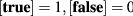and $(\cdot , \cdot )$ is the standard inner product in ${\mathbb {R}}^{r_i}$;

• a family of proximity relations

  $$\begin{aligned} {\mathscr {C}}_i \subset {\mathfrak {U}}_i \times X^{i+1} \end{aligned}$$

  (31)

  meaning that $(\xi , x) \in {\mathscr {C}}_i$ if an individual $\xi \in {\mathfrak {U}}_i$ is close enough to a deme with population vector $x \in X^{i+1}$.

In the sequel we shall use the following functions:

$$\begin{aligned} {{\,\mathrm{b}\,}}_i : X^i \ni x&\mapsto \min \left\{ \eta \in {\mathfrak {U}}_i : x^\eta> 0, {\mathfrak {f}}^i (\eta ) \le {\mathfrak {f}}^i (\zeta ) \right. \nonumber \\&\left. \qquad \text { for } \zeta \in {\mathfrak {U}}_i \text { such that } x^\zeta > 0 \right\} \in {\mathfrak {U}}_i \end{aligned}$$

(32)

that selects the best individual from the population x that has the minimal genotype according to any fixed ordering in ${\mathfrak {U}}_i$. We shall also use a kind of neighborhoods (proximity sets) related to the proximity relation:

$$\begin{aligned} C_i(\xi ) = \left\{ x \in X^{i+1} : (\xi , x) \in {\mathscr {C}}_i \right\} . \end{aligned}$$

(33)

A particular example of proximity relation (31) that is useful in practice can be found in [51].

4.3 HMS tree

The HMS populations form a hierarchy represented here by m-level undirected graph

$$\begin{aligned} HMSTREE = \langle V, E, F \rangle . \end{aligned}$$

The vertices V correspond to HMS populations (demes), the edges E follow the parent-child relation between populations. In our formal model we assume that this graph shows all the possible populations and does not change over time. Operations that in practice create new demes (i.e., the sprouting) here simply activate an available one. Similarly, the deme destruction (in the pruning) is here replaced with the deactivation. The number of children of each node can be different for different levels but at each level it is a constant $k_i$ ($i = 2, \ldots , m$). For the uniformity we set $k_1 = 1$. The labeling

$$\begin{aligned} F: V \rightarrow {\mathbb {N}}^m \end{aligned}$$

encodes the path from the root to a given node. Namely, let us take the set of admissible deme numbers at the tree level i

$$\begin{aligned} K_i = \{1, \dots , k_i\} \end{aligned}$$

and define

$$\begin{aligned} \begin{aligned} K^1&= \{ j^0 \} = \{ (1, \underbrace{0, \dots , 0}_{m - 1 \text { times}}) \}, \\ K^i&= \{ (1, j_2, \dots , j_i, \underbrace{0, \dots , 0}_{m - i \text { times}} ) : j_\kappa \in K_\kappa , \kappa = 2,\dots ,i\} \quad \text {for } i \ge 2, \\ K^m&= \{ (1, j_2, \dots , j_m) : j_\kappa \in K_\kappa , \kappa = 2,\dots ,m\}, \\ K&= \bigcup _{i = 1}^m K^i \subset {\mathbb {N}}^m, \\ K^{par}&= K \setminus K^m = \bigcup _{i=1}^{m-1} K^i. \end{aligned} \end{aligned}$$

(34)

Here, K is the domain of all labels (i.e., the image of F), $K^{i}$ is the set of labels of i-level demes, $K^{par}$ is the set of parental deme labels and $K^m$ is the set of leaf deme labels. In the sequel we shall use two auxiliary functions ${{\,\mathrm{len}\,}}: K \rightarrow \{1, \ldots , m\}$ returning the length of a path $j \in K$, i.e., the level of the deme with label j, and ${{\,\mathrm{prefix}\,}}_i : K \rightarrow K$ returning the length-i “prefix” of j. Namely

$$\begin{aligned}&\begin{aligned} {{\,\mathrm{len}\,}}(j)= \max \left\{ l \in \{ 1, \dots , m \} : j_l > 0 \right\} \\ &{{\,\mathrm{prefix}\,}}_i(j)= \left( j_1, \dots , j_i, 0, \dots , 0 \right) \in K^{\min \{ i, {{\,\mathrm{len}\,}}(j) \}}. \end{aligned} \end{aligned}$$

(35)

The root is obviously the unique node for which ${{\,\mathrm{len}\,}}(j) = 1$. Furthermore, for each parental node $j \in K^{par}$ (i.e., such that ${{\,\mathrm{len}\,}}(j) < m$) we can introduce the set of child node indices ${\mathscr {I}}_j$

$$\begin{aligned} {\mathscr {I}}_j = \left\{ \kappa \in K^{{{\,\mathrm{len}\,}}(j) + 1} : {{\,\mathrm{prefix}\,}}_{{{\,\mathrm{len}\,}}(j)} (\kappa ) = j \right\} . \end{aligned}$$

(36)

In the sequel we shall also make use of the set of all descendants of j together with j, i.e.,

$$\begin{aligned} {\mathscr {I}}^*_j = \left\{ \kappa \in K : {{\,\mathrm{prefix}\,}}_{{{\,\mathrm{len}\,}}(j)}(\kappa ) = j \right\} \end{aligned}\text{ .}$$

(37)

4.4 The HMS state space

First, note that the HGS model differs from the one presented in [51] in some points. To make the structure more flexible we have added a pruning operation. The latter consists in deactivating a stochastically selected sub-tree that was previously stopped, i.e., it exhausted its search capabilities. The pruning operation is already used in the computational practice and provides a probabilistic way to stop ineffective computations. In this manner it also enables us to prove the ergodicity of the whole strategy.

The overall state of the algorithm is determined by the states of all active and potentially active demes. All such demes are one-to-one related to nodes of the HMSTREE structure described in Sect. 4.3, hence they are also one-to-one related to the node indices, i.e., the elements of K. The state of a particular deme with label $j \in K$ is determined by its frequency vector $x \in X^{{{\,\mathrm{len}\,}}(j)}$. Moreover, each non-root deme has a status indicator that can have one of values ${\mathfrak {s}}_j \in \{inactive, new, active, stopped\}$. The root deme can only have status active or stopped.

At the beginning the only active deme is the root, all the other are set as inactive. An initial population of the root deme is generated by sampling with return from ${\mathfrak {U}}_1$ according to a given probability distribution.

Below we summarize the meaning of the status values.

• A deme is inactive if it has not been activated yet by the sprouting operation or was pruned previously. To make it entirely formal, we assume that the deme vector of each inactive deme at the level i has a fixed arbitrary value from $X^i$. This assumption affects neither the formal analysis nor the computational results in any way.

• A deme j is new if it has just been sprouted by its parental deme. A new deme cannot sprout another deme. The population of the new deme is sampled according to a given distribution, hence the population vector is set appropriately to a specific value (the initial setting is removed). The status changes from new to active or stopped after having executed the deme’s first metaepoch. In order to perform the sprouting the parental deme has to be active in at least one of the previous steps.

• A deme is active if it was new or active in the previous metaepoch and the stopping condition is not satisfied.

• A deme is stopped if the efficiency stopping condition is satisfied currently or was satisfied in the past, and the deme has not been pruned yet. In the case of a parental deme the status is also set to stopped when all its child demes have been activated (i.e., they have status active or stopped). Such a situation appears very rarely in the computational practice. The deme marked stopped once either stays stopped up to the end of computation and does not change its deme vector, or can be pruned with some positive probability.

Note that there are some relations among node status values and not all sequences of status values are possible. First, the HMS tree develops from the root towards leaves, hence if a deme is inactive, then all its descendants must bear the same status, i.e.,

$$\begin{aligned} {\mathfrak {s}}_j = inactive \Rightarrow {\mathfrak {s}}_\kappa = inactive \text { for } \kappa \in {\mathscr {I}}^*_j. \end{aligned}$$

This condition is naturally preserved by the pruning operation (cf. Algorithms 2–4). Second, the root is stopped if and only if all its children are not inactive.

Summing up, the HMS state space can be described in the following way:

$$\begin{aligned} \begin{aligned} X&= \biggl \{ \Bigl ( ({\mathfrak {s}}_j, x_j) \Bigr )_{j \in K} : x_j \in X^{{{\,\mathrm{len}\,}}(j)}, {\mathfrak {s}}_{j^0} \in \{ active, stopped\}, \biggr . \\&\qquad {\mathfrak {s}}_j \in \{ inactive, new, active, stopped \} \text { for } j \ne j^0, \\&\qquad {\mathfrak {s}}_j = inactive \Rightarrow {\mathfrak {s}}_\kappa = inactive \text { for } \kappa \in {\mathscr {I}}^*_j, \\&\qquad \biggl . {\mathfrak {s}}_{j^0} = stopped \Leftrightarrow {\mathfrak {s}}_\kappa \ne inactive \text { for } \kappa \in {\mathscr {I}}_{j^0} \biggr \}. \end{aligned} \end{aligned}$$

(38)

Note that an HMS state is a vector indexed by the elements of HMSTREE. Each component of this vector has in turn two sub-components: a deme population vector $x_j$ and a deme status ${\mathfrak {s}}_j$. Note also that X is finite provided all genetic universa ${\mathfrak {U}}_i$ are finite.

In the sequel we shall also need the following subsets of child node labels for $j \in K$ computed in a strategy state $\mathbf {x}\in X$.

$$\begin{aligned} \begin{aligned} {\mathscr {I}}_j^{in}(\mathbf {x})&= \left\{ \kappa \in {\mathscr {I}}_j : {\mathfrak {s}}_\kappa = inactive \right\} , \\ {\mathscr {I}}_j^{asn}(\mathbf {x})&= {\mathscr {I}}_j \setminus {\mathscr {I}}_j^{in}(\mathbf {x}), \\ {\mathscr {I}}_j^{s}(\mathbf {x})&= \left\{ \kappa \in {\mathscr {I}}_j : {\mathfrak {s}}_\kappa = stopped \right\} . \end{aligned} \end{aligned}$$

(39)

${\mathscr {I}}_j^{in}(\mathbf {x})$ is the set of labels of nodes that are active in state $\mathbf {x}\in X$, ${\mathscr {I}}_j^s(\mathbf {x})$ is the set of stopped node labels and ${\mathscr {I}}_j^{asn}(\mathbf {x})$ is the set of labels of nodes that are active, stopped or new. We shall also use the function returning the label of the inactive child of j that has the minimal number

$$\begin{aligned} {{\,\mathrm{mind}\,}}: X \times K^{par} \ni (\mathbf {x}, j) \longmapsto \mathop {{\mathrm{arg\,min}}}\limits _{\kappa \in {\mathscr {I}}_j^{in}(\mathbf {x})} \kappa _{{{\,\mathrm{len}\,}}(j) + 1} \in K. \end{aligned}$$

(40)

4.5 Algorithmic details

In this subsection we shall provide a detailed description of particular algorithms used in the HMS. It is based on the one presented in [51] but here we provide some clarifications and noteworthy modifications.

First of all, let us note that the strategy can be highly parallelized: the demes (sub-populations) can be evolved in parallel with some well-defined synchronization points. Moreover, the HMS structural operations (sprouting and pruning) can also be parallelized to some degree. Therefore, we shall formulate the overall strategy as three types of algorithms that are run concurrently: the root deme algorithm, the mid-level deme algorithm and the leaf deme algorithm. The latter two differ only in that the leaves do not perform actions related to children management.

We assume that in the initial state of the strategy, all demes except the root are inactive and the root itself is set to be active, i.e.,

$${\mathbf{x}}_{0} = {\text{ }}\left( {\left( {{\bar{\mathfrak{s}}}_{j} ,\bar{x}_{j} } \right)} \right)_{{j \in K}}$$

$\text {with } {\overline{{\mathfrak {s}}}}_{j^0} = active \text { and } {\overline{{\mathfrak {s}}}}_{j} = inactive \text { for } j \ne j^0.$The following auxiliary functions will be used as primitive building blocks of the algorithms presented in the sequel. They are explained here without details.

• —samples with return k times according to a probability distribution $\sigma$.

• —selects an element from list with the even probability.

• —returns indices of the children of deme, i.e. the elements of ${\mathscr {I}}_{deme}$, that have either of provided statuses (see (36)).

• —runs a metaepoch for the current deme, i.e., evolves population according to the transition matrix $Q_{level}^{kstep_{level}}$.

• —checks the global stopping condition.

• —checks the local stopping condition for deme.

Moreover, the algorithms use the functions ${{\,\mathrm{b}\,}}_i$ and ${{\,\mathrm{mind}\,}}$ introduced above, see (32) and (40), respectively.

The deme synchronization is based here on message-passing primitives. Namely we use two following operations:

• —a non-blocking operation of sending message to another deme;

• —a blocking operation of receiving message from another deme.

When there is a need to receive or send an object along with a message we use the overloaded functions and . The realization of and is a classical problem: their implementation can make use of, e.g., message queues.

Algorithm 2 shows the activity of the root deme. First, an initial population is sampled according to the distribution $\sigma _0$. Then, the main event loop is started. Its first stage is the execution of metaepochs in admissible subtrees followed by the execution of a metaepoch in the root itself. Note that during the first run of the loop there are no admissible subtrees, i.e., all children of the root are inactive. After the receipt of messages signaling metaepoch finishing the root checks the proximity of the best current individual to feasible children’s populations, initiates the sprouting in admissible subtrees and, if possible, sprouts a new branch from the current best individual. The completion of the sprouting in the subtrees is followed by the stochastic pruning of a stopped subtree. The decision of pruning is taken with probability $p_{prune}$: note that Binom(n, p) denotes the binomial distribution with parameters n and p. If the decision is positive, we select one of stopped children of the root and prune it, i.e., deactivate the children and all its successors. After the finish of the pruning the root checks if there are some inactive children. If not, the root status is set to stopped, otherwise it is set to active. The final stage of the loop is the evaluation of a global stopping condition of the whole strategy. If the latter is satisfied, the computations are finished and all the demes are halted in the appropriate order. Otherwise, the loop proceeds to the next run.

Next, let us consider a mid-level deme activity shown in Algorithm 3. After the initialization of the deme status and a loop control variable, the mid-level deme starts an event loop that consists of handling orders sent by the parent deme. The following order types are handled.

• ACTIVATE—the deme is initialized, i.e., its population is sampled according to the distribution $\sigma ^{seed}_{{{\,\mathrm{len}\,}}(j) - 1}$ and the deme status is set to new.

• PRUNE—the deme gets deactivated along with all its children.

• FINISH—the deme halts its computations and passes the message to all its children.

• RUNMETA—the deme passes the message to all its children and then runs its own metaepoch if its status is new or active; afterwards, the deme waits for the READY responses from all their children that signal the end of the children-deme metaepochs; subsequently, the local stopping condition is checked, which can change appropriately the deme status; finally, the READY message is sent to the parent.

• ISCLOSE—the deme checks if an individual sent from the parent is close to the current population, cf. (31).

• RUNSPROUT —if the deme’s children are not leaves they are requested to perform the sprouting; then, if the deme is active it performs the sprouting itself; next, it waits for the finish of the sprouting in the children; if there are no inactive children, the deme status changes to stopped; finally, the deme acknowledges the parent about the completion of the sprouting.

Finally, the activity of leaf demes is presented in Algorithm 4. Note that it is a simplified version of Algorithm 3 that omits all operations related to child management. To state it clearly, the event handling in leaves looks as follows.

• ACTIVATE —the population is sampled according to the distribution $\sigma ^{seed}_{m-1}$ and the deme status is set to new.

• PRUNE —the deme simply gets inactive.

• FINISH—the deme halts the evolution.

• RUNMETA—the deme runs its metaepoch if its status is new or active; afterwards, the local stopping condition is checked, which can change appropriately the deme status; finally, the READY acknowledgment is sent to the parent.

• ISCLOSE —the deme checks if an individual sent from the parent is close to the current population, cf. (31).

4.6 Transition operators related to HMS steps

The vast part of this subsection is a simplified version of the description provided in [51]. For the full details we refer the reader there. Note that the model presented in [51] uses the agent-based framework, hence such notions as “action” arise therein naturally. To highlight the correspondence between the current model and the older one we preserve the basic terminology, at the same time not retaining agents themselves. Therefore, in the sequel “action” has exactly the same meaning as “operation”.

4.6.1 General structure of operators

An HMS action $\alpha$ is here represented as a pair of functions $\left( \delta _\alpha , \vartheta _\alpha \right)$. The first of them

$$\begin{aligned} \delta _\alpha : X \rightarrow ~[0, 1] \end{aligned}$$

(41)

is the decision function. It computes the probability of choosing the action $\alpha$ in state $\mathbf {x}\in X$, i.e., $\alpha$ is run with probability $\delta _\alpha (\mathbf {x})$ and rejected with probability $1 - \delta _\alpha (\mathbf {x})$. The state transition function

$$\begin{aligned} \vartheta _\alpha : X \rightarrow {\mathfrak {M}}(X) \end{aligned}$$

(42)

defines a non-deterministic state transition resulting from the execution of $\alpha$: $\vartheta _\alpha (\mathbf {x})(\mathbf {y})$ gives the probability of changing state from x to y as the result of $\alpha$. A trivial yet important example of such an action is the no-op (do-nothing action) denoted here null. Its state transition function is the Kronecker delta, i.e.,

$$\begin{aligned} \vartheta _{null}(\mathbf {x})(\mathbf {y})= {\left\{ \begin{array}{ll} 1 &{} \text {if } \mathbf {x}= \mathbf {y}\\ 0 &{} \text {otherwise}. \end{array}\right. } \end{aligned}$$

(43)

The overall Markov kernels related to any action $\alpha$ can be computed using the chain rule. It has the following form.

$$\begin{aligned} \varrho _\alpha (\mathbf {x})(\mathbf {y}) = \delta _\alpha (\mathbf {x}) \cdot \vartheta _\alpha (\mathbf {x})(\mathbf {y}) + \left( 1 - \delta _\alpha (\mathbf {x}) \right) \cdot \vartheta _{null}(\mathbf {x})(\mathbf {y}). \end{aligned}$$

(44)

The first term on the right-hand side is connected to the state transition when the decision of executing $\alpha$ is positive. The second term represents the case of the rejection of $\alpha$ when in fact we do not perform any state transition.

In the sequel we show decision functions and state-transition functions for the following non-trivial action types:

• metaepoch actions $\left\{ meta_j : j \in K \right\}$ available for all demes;

• sprouting actions $\left\{ sprout_j : j \in K^{par} \right\}$ defined only for the parental demes;

• pruning action prune available for the root deme.

4.6.2 Metaepoch operators

Now let us recall the stochastic operators for the $meta_j$ action. To this end let us consider two consecutive states $\mathbf {x}, \mathbf {y}\in X$ appearing during the HMS computation. We will denote by $({\mathfrak {s}}_j, x_j)$ the components of $\mathbf {x}$ and by $({\mathfrak {t}}_j, y_j)$ the components of $\mathbf {y}$.

The decision function for the root deme $j^0$ is given by the following formula

$$\begin{aligned} \delta _{meta_j}(\mathbf {x}) = {\left\{ \begin{array}{ll} 1 &{} \text {if } {\mathfrak {s}}_{j^0} = active,\\ 0 &{} \text {otherwise}. \end{array}\right. } \end{aligned}$$

(45)

For lower-level demes $j \in K \setminus K^1$ the decision function has the form

$$\begin{aligned} \delta _{meta_j}(\mathbf {x}) = {\left\{ \begin{array}{ll} 1 &{} \text {if } {\mathfrak {s}}_j = active \text { or } {\mathfrak {s}}_j = new,\\ 0 &{} \text {otherwise}. \end{array}\right. } \end{aligned}$$

(46)

Now let us proceed to the state transition function for $meta_j$. To this end denote $i = {{\,\mathrm{len}\,}}(j)$. Then we have

$$\begin{aligned}&\vartheta _{meta_j}(\mathbf {x})(\mathbf {y}) \nonumber \\&\quad = \left( Q_i^{kstep_i} \right) _{x_j, y_j} \nonumber \\&\qquad \cdot {\left\{ \begin{array}{ll} S_i(x_j) \left[ \left( {\mathfrak {f}}^i, x_j - y_j \right) < {{\,\mathrm{lsc}\,}}_i \right] & \text {if } {\mathfrak {t}}_j = stopped \text { and } \\ &{\mathfrak {s}}_\kappa = {\mathfrak {t}}_\kappa , x_\kappa = y_\kappa \text { for } \kappa \ne j,\\ (1 - S_i(x_j)) \left[ \left( {\mathfrak {f}}^i, x_j - y_j \right) \ge {{\,\mathrm{lsc}\,}}_i \right] &\text {if } {\mathfrak {t}}_j = active \text { and } \\ & {\mathfrak {s}}_\kappa = {\mathfrak {t}}_\kappa , x_\kappa = y_\kappa \text { for } \kappa \ne j,\\ 0 & \text {otherwise.} \end{array}\right. } \end{aligned}$$

(47)

4.6.3 Sprouting operators

First let us introduce the following family of stochastic functions:

$$\begin{aligned} {\mathscr {T}}_i : X_i \longrightarrow {\mathfrak {M}}( X_{i+1} ), \quad i = 1, \ldots , m-1, \end{aligned}$$

(48)

where ${\mathscr {T}}_i(x)$ is the distribution of $\mu _{i+1}$-times sampling with return from ${\mathfrak {U}}_{i+1}$ according to the distribution $\sigma _i^{{{\,\mathrm{b}\,}}_i(x)}$. To simplify the formulae defining operators let us introduce another auxiliary function

$$\begin{aligned} a : X \times K^{par} \ni (\mathbf {x}, j) \longmapsto {{\,\mathrm{card}\,}}{\mathscr {I}}_j^{in}(\mathbf {x}) \in {\mathbb {N}}, \end{aligned}$$

Using the above-defined notions we can formulate the decision function for the sprouting in demes $j \in K^{par}$

$$\begin{aligned} \delta _{sprout_j}(\mathbf {x}) = {\left\{ \begin{array}{ll} 1 &\quad \text {if } s^j = active \text { and } \left( {{\,\mathrm{b}\,}}_i(x_j), x_\kappa \right) \not \in {\mathscr {C}}_i \text { for } \kappa \in {\mathscr {I}}_j^{asn}(\mathbf {x}), \\ 0 &\quad \text {otherwise}\\ \end{array}\right. } \end{aligned}$$

(49)

Similarly we obtain the following form of the state-transition function for the sprouting.

$$\begin{aligned} \vartheta _{sprout_j}(\mathbf {x})(\mathbf {y}) = {\left\{ \begin{array}{ll} {\mathscr {T}}_{{{\,\mathrm{len}\,}}(j)} (x_j)(y_{{{\,\mathrm{mind}\,}}(\mathbf {x}, j)}) &\quad \text {if } \biggl ( \bigl ( z^j = active \text { and } a(\mathbf {x}, j) > 1 \bigr ) \text { or } \biggr . \\ &\quad \biggl . \bigl ( z^j = stopped \text { and } a(\mathbf {x}, j) = 1 \bigr ) \biggr ) \text { and } \\ &\quad {\mathfrak {t}}_{{{\,\mathrm{mind}\,}}(\mathbf {x}, j)} = new \text { and } \\ &\quad {\mathfrak {s}}_\kappa = {\mathfrak {t}}_\kappa , y_\kappa = x_\kappa \text { for } \kappa \ne {{\,\mathrm{mind}\,}}(\mathbf {x},j),\\ 0 &\quad \text {otherwise.} \end{array}\right. } \end{aligned}$$

(50)

4.6.4 Pruning operator

Now, let us proceed to the pruning operator. Note that this definition cannot be found in [51] because the model presented in that paper does not include the pruning. The decision function in our case has the following form.

$$\begin{aligned} \delta _{prune}(\mathbf {x}) = {\left\{ \begin{array}{ll} p_{prune} &\quad \text {if } {\mathscr {I}}^s_{j^0}(\mathbf {x}) \ne \emptyset , \\ 0 &\quad \text {otherwise}. \end{array}\right. } \end{aligned}$$

(51)

The state transition function can be expressed as follows

$$\begin{aligned} \vartheta _{prune}(\mathbf {x})(\mathbf {y}) = {\left\{ \begin{array}{ll} \frac{1}{{{\,\mathrm{card}\,}}\left( {\mathscr {I}}^s_{j^0}(\mathbf {x}) \right) } &\quad \text {if } \mathbf {y}\in PB_j(\mathbf {x}) \text { for some } j \in {\mathscr {I}}^s_{j^0}(\mathbf {x}), \\ 0 &\quad \text {otherwise} \\ \end{array}\right. } \end{aligned}$$

(52)

where

$$\begin{aligned} PB_j(\mathbf {x})= & \quad \left\{ \mathbf {y}\in X : {\mathfrak {t}}_\kappa = inactive, y_\kappa = {\overline{x}}_{\kappa } \right. \\&\left. \text { for } \kappa \in {\mathscr {I}}^*_j, {\mathfrak {t}}_\lambda = {\mathfrak {s}}_\lambda , y_\lambda = x_\lambda \text { for } \lambda \not \in {\mathscr {I}}^*_j \right\} \end{aligned}$$

4.7 The transition probability function for the whole HMS

First, let us recall that the superposition of two Markov kernels

$$\begin{aligned} \varrho ^1, \, \varrho ^2: X \rightarrow {\mathfrak {M}}(X), \end{aligned}$$

(53)

can be computed using the total probability law:

$$\begin{aligned} \varrho ^2 \circ \varrho ^1 (\mathbf {x})(\mathbf {y}) = \sum _{\mathbf {u} \in X} \varrho ^1(\mathbf {x})(\mathbf {u}) \ \varrho ^2(\mathbf {u})(\mathbf {y}). \end{aligned}$$

(54)

In [51] we showed that if two actions $\alpha _1$, $\alpha _2$ are either both metaepoch actions or both sprouting actions their kernels commute, i.e,

$$\begin{aligned} \varrho _{\alpha _1} \circ \varrho _{\alpha _2} = \varrho _{\alpha _2} \circ \varrho _{\alpha _1}, \end{aligned}$$

which means that the outcome of the actions’ execution is independent upon their order. Therefore, as in Algorithms 2–4 they can be safely run in parallel.

The Markov kernel for the whole metaepoch step $\tau _{meta}: X \rightarrow {\mathfrak {M}}(X)$ is the superposition of single-deme metaepoch Markov kernels $\varrho _{meta_j}$ for all demes $j \in K$:

(55)

Note that according to what has been written above the superposition in (55) does not depend on an order of labels in K. Similarly, the Markov kernel for the sprouting step $\tau _{sprout}: X \rightarrow {\mathfrak {M}}(X)$ is the superposition of single-deme Markov kernels $\varrho _{sprout_j}$ for all parental demes $j \in K^{par}$. Therefore

(56)

Here, again, the superposition is not sensitive to deme ordering.

The synchronization scheme used in Algorithms 2–4 divides each global step of the HMS into three subsequent stages: the metaepoch stage, the sprouting stage and the pruning stage. Therefore, the transition function for the whole strategy $\tau : X \rightarrow {\mathfrak {M}}(X)$ is the superposition of the respective Markov kernels, i.e.,

$$\begin{aligned} \tau = \varrho _{prune} \circ \tau _{sprout} \circ \tau _{meta}. \end{aligned}$$

(57)

4.8 HMS asymptotic analysis

In this subsection we consider an important asymptotic property of the whole strategy, i.e., its ergodicity, which can be understood as the guarantee of success, in the sense that if a complex dynamical system as HMS can reach any of its states in a finite number of steps, it can end up in any desired state in finite time.

Theorem 1

Assume that for every $i = 1, \dots , m$

$(H^1_{stop})$:

the stopping conditions (30) are not trivial, i.e., the genetic universa ${\mathfrak {U}}_i$, the fitness functions ${\mathfrak {f}}^i$ and the thresholds ${{\,\mathrm{lsc}\,}}_i$ are such that for each $x \in X^i$ we have

$$\begin{aligned} 0< \Pr \left\{ y \in X^i : \left( {\mathfrak {f}}^i, x - y \right)< {{\,\mathrm{lsc}\,}}_i \right\} < 1; \end{aligned}$$

$(H^2_{stop})$:

the global stopping condition is trivial, i.e., it cannot be satisfied;

$(H_{evo})$:

the evolution in each deme is an ergodic Markov chain such that the metaepoch transition matrix $Q_i^{kstep_i}$ is positive;

$(H_{prune})$:

the pruning is probable but not certain, i.e., $0< p_{prune} < 1$;

$(H^1_{prox})$:

the proximity relations ${\mathscr {C}}_i$ are not trivial, i.e., for every $\xi \in {\mathfrak {U}}_i$

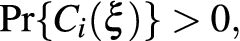
$(H^2_{prox})$:

the proximity relations ${\mathscr {C}}_i$ are such that the sprouting is always possible provided not all child indices are used, i.e., for every $k < k_i$, $j \in K^i$ and every $\xi _1, \dots , \xi _k \in {\mathfrak {U}}_{i}$

Then the Markov chain with transition function (57) is ergodic.

Proof

To prove the ergodicity of the considered chain we need to show its irreducibility and aperiodicity.

Recall that the irreducibility means that any two states $\mathbf {x}, \mathbf {y}\in X$ communicate, i.e., we can pass from $\mathbf {x}$ to $\mathbf {y}$ in a finite number of steps with positive probability. The proof shall proceed by showing that all elements of X are reachable from ${\mathbf {x}}_0$ and that ${\mathbf {x}}_0$ is reachable from any other state.

Let us start with the second claim. Let ${\mathbf {x}}$ be an arbitrary state. First observe that if the root has some children that are not inactive (i.e., they are new, active or stopped) any of them can be deactivated by means of the pruning operation in the following sequence of steps:

• 1. If it is new or active We execute a metaepoch (and possibly the sprouting) such that the local stopping condition gets satisfied and the status changes to stopped;

• 2. We prune the stopped child.

Step 1 has positive probability because it is a chain of positive-probability events. Namely, thanks to assumption $(H_{evo})$ we can pass between arbitrary elements of $X^i$ in one metaepoch with positive probability and thanks to assumption $(H^1_{stop})$, the probability that the reached population satisfies the local stopping condition is also positive. After the completion of step 1 the probability of running the pruning action is positive, see (51), and the probability of selecting the considered child is also positive, see (52). Therefore, the chain rule implies that the deactivation of the child deme in a finite number of steps has a positive probability.

Next, observe that, as long as there are the root’s children that are not inactive, with positive probability we can repeatedly prune stopped demes without sprouting any new children between two subsequent deactivations. This means that the event of not sprouting a new deme after pruning a stopped one has the positive probability provided there are not-inactive children of the root. But thanks to assumptions $(H_{evo})$ and $(H^1_{prox})$ this is a positive-probability event: a metaepoch in the root ending up with the best individual that falls close to any of not-inactive children.

This way, with positive probability we can prune all-but-one children of the root. The next step is that we evolve the root finishing in ${\overline{x}}_{j^0}$ at the same time pruning the last child. Such an event has a positive probability as well due to assumptions $(H_{evo})$, $(H_{prune})$ and $(H^2_{stop})$. Therefore, we have shown the way to pass from an arbitrary state $\mathbf {x}\in X$ to $\mathbf {x}_0$ in a finite number of steps with positive probability.

To proceed the opposite way, take an arbitrary $\mathbf {x}\in X$ and consider the following chain of possible events:

• 1. We start in $\mathbf {x}_0$ evolving the root in such a way that we sprout the number of children that equals the maximal child number at level 2 in $\mathbf {x}$,

• 2. We proceed the same way at lower levels at the same time pruning the branches that are inactive in $\mathbf {x}$,

• 3. We evolve the not-inactive branches to reach the same status and population as in $\mathbf {x}$.

The above events have positive probability thanks to our assumptions, which shows that we can pass from $\mathbf {x}_0$ to $\mathbf {x}$ with positive probability.

To conclude the proof, we need to prove the aperiodicity of the chain, which, thanks to the irreducibility, is equivalent to the aperiodicity of any of its states. To this end, take $\mathbf {x}\in X$ such that ${\mathfrak {s}}_j = stopped$ for all $j \in K$. Then no sprouting is possible because all demes are busy and no deme evolution occurs because all demes are stopped. Hence, as long as the pruning does not happen, which has positive probability thanks to $(H_{prune})$, the state does not change, which means that $\mathbf {x}$ is aperiodic. $\square$

Remark 9

Assumption $(H_{evo})$ is satisfied for both SGA with positive mutation and MWEA (see Sects. 2 and 3).

Remark 10

For some natural proximity relations assumptions $(H^1_{prox})$ and $(H^2_{prox})$ reduce to geometric constraints on the neighborhoods $C_i$ with respect to the computational domain. This is, e.g., the case of proximity relation defined in [51] where the neighborhoods are discretizations of balls in ${\mathbb {R}}^n$ that must have sufficiently small diameters in order to satisfy $(H^2_{prox})$.

5 Illustrative examples

The essential, qualitative results of this paper are presented in the preceding sections. Here, we mean to present in action the strategies which are supported by these formal postulates. We have carefully chosen these simulations from our previous publications [47, 48], refining their results.

In particular, we will show two benchmark cases, followed by an engineering example. The first benchmark will use a fitness function with 4 non-convex regions of insensitivity. We will show how particular stages of the algorithm up to the local approximation work on this example. The second will use a fitness function with similar features, but with more regions of insensitivity—we present a comparison based on metrics for this case. In both benchmarks insensitivity regions and their approximations are constructed as level sets with cutoff 0.1, i.e. subsets of the domain where the objective function (or its approximation) assumes values less than 0.1. We will finish with the engineering example from the domain of underground hydrocarbon prospecting.

5.1 Benchmark with 4 regions of insensitivity

The first example consists in finding the shapes of the four insensitivity regions, which objective function is shown in Fig. 4 on the left, and it is meant to present the mechanics of the strategy. The strategy is composed of the global phase and the local phase with MWEA. In the global phase we use HMS-CMA-ES [46], and compare it with NEA2 [38]. The former is supported by the Markov analysis we presented earlier in the paper, and the latter is a state-of-the-art algorithm dedicated to multimodal problems. For more details about the objective function and the configuration, see [48, Sect. 3.1].

Fig. 4

The plots of the first and the second benchmark functions in their domains [48, Fig. 1]

We show the results of running both variants of the strategy in Fig. 5. In the first row, there are clusters returned by the global phases. HMS-CMA-ES produces more focused samples, which better identify the lowlands. The clusters laying in the same basins of attraction, based on the hill-valley rule, are in the second row. For NEA2, this operation results in clusters that do not separate lowlands. In the final row, we show MWEA demes populations. For HMS-CMA-ES clusters, MWEA explores the neighborhoods of the lowlands, possibly allowing shape approximation, maintains separation and reducing overall number of evaluations. However, MWEA does not handle NEA2 clusters well: although lowland neighborhoods are explored, the lowlands are not separated, and it results in expendable objective evaluations.

Fig. 5

The strategy steps visualised for NEA2 and HMS-CMA-ES global phase [48, Fig. 2]. Steps are presented in consecutive rows: clusters after the global phase, clusters after reduction and points obtained by MWEA. The clusters from the first row are not exhaustive to keep the plots readable. Each cluster is shown with a different mark type and the solid lines are 0.1 isolines of the fitness function

5.2 Benchmark with 25 regions of insensitivity

Here, we present how the two variants of the strategy (NEA2 and HMS-CMA-ES based) perform on a benchmark with more lowlands, compared to the previous case. We show its objective function in Fig. 4 on the right. In this example, we perform calculations with evaluation budget varying from 2000 to 10000. After its exhaustion, the global phase is stopped and only the local phase continues, see [48, Sect. 3.2].

Fig. 6

Metric values for NEA2 and HMS-CMA-ES variants in the second case. The data points are shown for budgets ranging from 2000 to 10000 evaluations. Each point is an average of the metric value for 10 runs of each configuration. The error bars depict the maximum and the minimum value among these 10 runs

Figure 6 displays the results of the global and local phases. On the graphs, three metrics are shown in function of the budget: number of clusters after the global phase, after reduction and the ratio of covered regions. For a well-tuned strategy, we expect the number of clusters to reflect the number of lowlands, especially after the reduction. The higher the region coverage ratio, the better. Unfortunately, the NEA2 features indicated in the previous example make it ineffective at identifying a larger number of lowlands —the non-separated clusters are merged into a single one. HMS-CMA-ES fares much better in that regard, yielding also a higher region coverage ratio.

Table 1 Average Hausdorff distances between the exact sets of insensitivity and their approximations [48, Tab. 1]

We also compare the quality of the lowland shape approximation with different methods: kriging, $L^2$-projection and $H^1$-projection. In Table 1 we collect Hausdorff distances of the approximations from the exact lowlands. Kriging achieves the best accuracy, with $L^2$-projection closely behind. The samples obtained from using NEA2 prevent obtaining good approximations for any approximation algorithm.

Fig. 7

Each graph presents contours of the insensitivity region generated by approximation methods compared to the exact contour [48, Fig. 4]. We show $L^2$-projection, $H^1$-projection and kriging methods

For illustration, we present an example of the shape approximations for different approximation and global phase algorithms in Fig. 7. The approximations resulting from HMS-CMA-ES are better than NEA2 in general, and deficiency of the $H^1$-projection is evident.

5.3 Engineering example

The magneto-telluric (MT) method [10, 63] is a geophysical prospecting method which is used to determine the resistivity distribution in the Earth crust. It exploits the telluric currents induced by the solar wind, modeling the electromagnetic field. The underground formation influences these currents, which in turn are measured indirectly by antennae placed at the surface of Earth or its seafloor. This feature makes it possible to invert such measurements to obtain the unknown resistivity distribution. Being clean and inexpensive, it has been applied for different purposes, such as mapping of active faults [29], the study of volcanoes [21], and exploration of offshore hydrocarbons [66].

Figure 8 describes the selected Earth model for the MT problem. The computational domain consists of air and a 1D layered media where a 2D heterogeneity (grey rectangle) is embedded in one of the layers. The blue rectangle corresponds to the natural source in the ionosphere, while the red triangles correspond to the receivers at the Earth’s surface. The physical domain is truncated with a Perfectly Matched Layer (PML) complemented with a Dirichlet homogeneous border condition imposed on its outer part, and $hp-$FEM solves the problem, see [2] and [57, Sect. 3] for more details.

The task is to identify the resistivities of the subsurface regions presented in Fig. 8. We take the computation domain of the problem ${\mathscr {D}}=[0,6]^4$, to be able to apply HMS. The points from the computation domain are mapped to the resistivities by a function .

The resistivities depend on the type of subsurface region. Example approximate values of resistivities are: water ${1}\,\Omega \text {m}$, rock ${1000}\,\Omega \text {m}$, oil ${20}\,\Omega \text {m}$, shale ${5}\,\Omega \text {m}$.

We calculate the misfit for a single wave frequency $\nu _1=10^{-1.2}\,\text {Hz}$. Such a choice ensures sufficient penetration of the waves into the subsurface (in terms of depth) while maintaining resolution, see, e.g. [63].

Fig. 8

The domain of the MT computation [47, Fig. 4]

In this case, in the global phase we only used HMS. For configuration and other details, see [47, Sect. 3.4].

Fig. 9

MT local phase test, a combined sample from all the LBA runs [47, Fig. 5]. Selected dimensions are plotted, including misfit and a projection of points with misfit below $10^{-10}$ in gray

The best misfit values in most of the demes fluctuate around $10^{-11}$ and the median is around $10^{-9}$, which misfit level is comparable to results obtained when solving similar problem in [57]. In Fig. 9, all points from the local phases are shown. An insensitive region in $x_4$ dimension is clearly visible.

Some of the demes returned from the global phase contained individuals, which were within the range 0.3 in the 4D space from the real resistivity parameter vector, which was around the best achieved distance. In particular, the solution with best approximation of the $\rho _3$ value, that also had the misfit of a degree $10^{-10}$, was within $10^{-3}$ of the real $\rho _3$ value. So, the extracted clusters, which we created based on demes, inherited information about the subregion which may contain oil. However, such evaluation is an a posteriori claim. Because of the ill-conditioning, we cannot distinguish which points with good misfit values correspond to the real resistivity parameters, however, the real parameters can be extracted with further informed analysis of the lowland regions.

As a reference solution for the assessment of the local phase, we use an approximation based on evaluations gathered from multiple MT experiments (over 80,000 evaluations with different precision levels, 2000 chosen to cover the domain with the highest available precision solutions). For this test, we have identified 30 individual lowland regions by computing a level set of such an approximation of misfit, one of which contained the real resistivity parameters vector.

The statistics of the approximation errors for all the LBAs are presented in Table 2. Moreover, for each LBA, we calculate two dedicated coverage metrics, shown in Table 3. For each LBA, we determine the points which lie within the obtained lowland approximation (with either $L^2$ projection, $H^1$ semi-projection, or kriging), let us call them approximation points.

Firstly, we verified if each LBA covered the real resistivity parameters vector by checking if any of its approximation points lies within the distance 0.3 from the vector. Then, we calculated the percentage of the runs, that had such an LBA, and we show its values under name coverage of real parameters (column 2, Table 3).

For calculating the second metric we use the reference points, which are inside a particular reference lowland. Then, for each reference lowland we calculate how well the approximation points cover it, which is done by checking if a point from the reference lowland lies within the distance 0.1 from an approximation point. The lowland coverage equals to the percent of the reference points covered. The best lowland coverage is then the best coverage from the 30 reference lowlands (column 3, Table 3).

Kriging achieves the best lowland coverage in these results, but the results are too uncertain to make stronger claims.

Table 2 MT local phase test, approximation errors [47, Tab. 6]

Table 3 MT local phase test, coverage results

6 General conclusions

• 1. The stochastic population-based search with a dynamic sampling measure adaptation, that can be modeled as a stationary Markov chain, might be treated as a machine learning process that gathers more and more information about the problem with each iteration. If the family of such searches has a focusing heuristic (see Definition 6), then we may conjecture, that the maximum information about the problem is contained in the set ${\mathscr {K}}$ of fixed points of heuristic, that are the frequency vectors of the limit populations representing most exhaustive searches (infinite sample after infinite number of steps) (see Remarks 4.1 and 4.2). Notice, that typically ${\mathscr {K}}$ is a singleton.

• 2. The above reasoning shows us, that in order to solve $\varPi _1, \varPi _2$ (see Definition 5) we really expect to obtain a random sample with a probability distribution sufficiently close to at least one fixed point of heuristic, i.e. falling into $\varepsilon$—convex envelope ${\mathscr {K}}_\varepsilon$ of the fixed points, for a sufficiently small $\varepsilon$. The analysis of dynamic and asymptotic features of sampling measures, seems to be more adequate in such case, than behavior analysis of single, selected individuals (e.g. best fitted ones) in the consecutive populations, as it is performed in the classical approaches (see Remark 6.2).

• 3. If the Markov chain modeling the search is ergodic, than it ensures the asymptotic guarantee of success i.e. the well approximation of fixed point of heuristic ${\mathscr {K}}_\varepsilon$ can be reached in a finite number of steps, starting from an arbitrary $x_0 \in X_\mu$, if $\mu$ is sufficiently large, so that ${\mathscr {K}}_\varepsilon \cap X_\mu \ne \emptyset$ (see Remark 6.3).

• 4. If we apply the family of “well tuned” searches to solve the ill-conditioned problems $\varPi _1, \varPi _2$, then we can draw the information about lowlands and minimum manifolds by the proper post-processing of the limit population $x_K$ or the cumulative population $\frac{1}{K}\sum _{t=1}^K x_t$, where K is a sufficiently large number of steps and $x_K \in X_\mu$ for sufficiently large $\mu$. Such post-processing may consist in clustering, cluster separation analysis, local fitness approximation, etc. (see Remarks 4.3, 6.1 and 6.2).

• 5. The possible concept of stopping a stochastic strategy solving such problems is to recognize, whether at least one population vector $x_t \in X_\mu$ falls into the set of states ${\mathscr {K}}_\varepsilon$. More formally, we may evaluate the proper statistic of the FHT of the set ${\mathscr {K}}_\varepsilon \cap X_\mu$. In particular, FHT expectation might be computed from the linear system (8) (see Remarks 6.4, 6.5). The other, more practical possibility of verifying a stopping condition is to check, whether the consecutive samples form clusters of a sufficiently high quality, i.e. sufficiently dense and well separated from each other (see Remark 6.6).

• 6. Assessing whether the particular family of searches is “well tuned” is difficult in the computational practice (see Remark 6.8). Typically, the algorithms with a stronger selection pressure are more likely “well tuned”. Unfortunately, such algorithms are ineffective in a global search. The possible solution is to use a cascade of stochastic searches, in which the upper ones are designated to global search, while the lowest ones deliver the sample concentrated in the basins of attraction of lowlands or minimum manifolds. Such proposition called HMS/MWEA was presented later in Sect. 4.

• 7. We have proven that the HMS/MWEA strategy has the asymptotic guarantee of success in the sense that it can reach any of its states in a finite number of steps with positive probability (see Sect. 4). Therefore, we can expect that when run sufficiently long, the strategy will produce populations in leaf demes that will occupy significant parts of interesting regions. However mostly theoretical, this result forms a solid foundation for the confidence in the HMS/MWEA search capabilities.

• 8. In Sect. 5, the computational examples display how the HMS/MWEA strategy performs on benchmarks and in an engineering case. The strategy behaves as expected from the previous Markov chain analysis. The search is focused in the vicinity of the lowland regions. Thanks to this, decent lowland shapes approximations are then obtained. We also determine lowland regions of the engineering example’s misfit function. This case proves more challenging, nevertheless, correctness of the obtained solution is retained.

• 9. Currently, it is impossible to provide a comprehensive comparison of the presented strategy with respect to state-of-the-arts strategies. The reason is that the aim of our strategy is the insensitivity region approximation, which is illustrated in Sect. 5, and possible competitors, like those described in [15, 32, 38], concentrate on finding the global minimizers or even a single global minimizer. Despite that, in Sect. 5 we compare the performance of our strategy with algorithms that provide partial coverage of its functionality. In particular, we compare its global phase with NEA2 [38] and its local-approximation phase with kriging method [24] (see Figs. 6, 7 and Tables 6–3).

References

Alden W, Greg C (2004) Bistability of the needle function in the presence of truncation selection. In: Deb K (ed) GECCO 2004, Lecture Notes in Computer Science, vol 3103. Springer, Berlin, pp 330–342
Álvarez-Aramberri J, Pardo D (2017) Dimensionally adaptive hp-finite element simulation and inversion of 2d magnetotelluric measurements. J Comput Sci 18:95–105
Arabas J (2012) Approximating the genetic diversity of populations in the quasi-equilibrium state. IEEE Trans Evol Comput 16:632–644. https://doi.org/10.1109/TEVC.2011.2166157
Barabasz B, Migórski S, Schaefer R, Paszyński M (2011) Multi-deme, twin adaptive strategy hp-hgs. Inverse Probl Sci Eng 19(1):3–16
Beume N, Laumanns M, Rudolph G (2010) Convergence rates of (1+1) evolutionary multiobjective optimization algorithms. In: Schaefer R, Cotta C, Kołodziej J, Rudolph G (eds) Parallel problem solving from nature— PPSN XI, vol 6238. Lecture notes in computer science. Springer, Berlin, pp 597–606
Byrski A, Schaefer R, Smołka M, Cotta C (2013) Asymptotic guarantee of success for multi-agent memetic systems. Bulletin of the polish academy of sciences: technical sciences 61(1):257–278
Cabib E, Davini C, Chong-Quing R (1990) A problem in the optimal design of networks under transverse loading. Quarterly of Appl. Math. 48(2):251–263
Cabib E, Schaefer R, Telega H (1998) A parallel genetic clustering for inverse problems. Lect Notes Comput Sci 1541(2):551–556
Caicedo JM, Yun G (2011) A novel evolutionary algorithm for identifying multiple alternative solutions in model updating. Struct Health Monit 10:491–501
Chave A, Jones A (2012) The magnetotelluric method: theory and practice. Cambridge University Press, Cambridge
Dixon LCW, Szegö GP (eds) (1975) Toward global optimization. North Holland, Amsterdam
Duan Q, Sorooshian S, Gupta V (1992) Effective and efficient global optimization for conceptual rainfall-runoff models. Water Resour Res 28(4):1015–1031
Faliszewski P, Sawicki J, Schaefer R, Smołka M (2017) Multiwinner voting in genetic algorithms. IEEE Intell Syst 32(1):40–48. https://doi.org/10.1109/MIS.2017.5
Faliszewski P, Smołka M, Schaefer R, Paszyński M (2016) On the computational cost and complexity of stochastic inverse solvers. Comput Sci 17(2):225–264. https://doi.org/10.7494/csci.2016.17.2.225
Fan Q, Meng X, Xu C, Yu J (2020) Solution method for ill-conditioned problems based on a new improved fruit fly optimization algorithm. J Appl Geodesy 14(1):55–64. https://doi.org/10.1515/jag-2019-0025
Gajda E, Schaefer R, Smołka M (2010) Evolutionary multiobjective optimization algorithm as a Markov system. In: Schaefer R, Cotta C, Kołodziej J, Rudolph G (eds) Parallel problem solving from nature—PPSN XI, vol 6238. Lecture notes in computer science. Springer, Berlin, pp 617–626
Gajda-Zagórska E, Schaefer R, Smołka M, Paszyński M, Pardo D (2014) A hybrid method for inversion of 3D DC logging measurements. Nat Comput 14(3):355–374. https://doi.org/10.1007/s11047-014-9440-y
Garipov T, Izmailov P, Podoprikhin D, Vetrov DP, Wilson AG (2018) Loss surfaces, mode connectivity, and fast ensembling of DNNs. In: Bengio S, Wallach H, Larochelle H, Grauman K, Cesa-Bianchi N, Garnett R (eds) Advances in neural information processing systems, vol 31. Curran Associates Inc, Red Hook, pp 8789–8798
Ghosh S, Das S, Vasilakos AV, Suresh K (2012) On convergence of differential evolution over a class of continuous functions with unique global optimum. IEEE Trans Syst Man Cybern Part B (Cybernetics) 42(1):107–124. https://doi.org/10.1109/TSMCB.2011.2160625
He J, Yao X (2003) Towards an analytical framework for analysing the computation time of evolutionary algorithms. Artif Intell 145:59–97. https://doi.org/10.1016/S0004-3702(02)00381-8
Hill G, Wannamaker P, Stodt J, Unsworth M, Maris V, Bedrosian P, Wallin E, Kordy M, Ogawa Y, Kyle P, et al. (2017) Imaging the magmatic system of erebus volcano, antarctica using the magnetotelluric method. In: AGU fall meeting abstracts
Isakov V (2006) Inverse problems for partial differential equations. Springer, Berlin
Isshiki M, Sinclair D, Kaneko S (2006) Lens design: global optimization of both performance and tolerance sensitivity. In: International optical design, p. TuA5. Optical Society of America. https://doi.org/10.1364/IODC.2006.TuA5. http://www.osapublishing.org/abstract.cfm?URI=IODC-2006-TuA5
Jin Y (2005) A comprehensive survey of fitness approximation in evolutionary computation. Soft Comput 9(1):53–59
Karcz-Dulęba I (2001) Dynamics of infinite populations evolving in a landscape of uni- and biomodal fitness functions. IEEE Trans Evol Comput 5:398–409. https://doi.org/10.1109/4235.942533
Karcz-Dulęba I (2006) Dynamics of two-element populations in the space of population states. IEEE Trans Evol Comput 10:199–209. https://doi.org/10.1109/TEVC.2005.856070
Kazimierz G (1996) On asymptotic properties of a selection-with-mutation operator. In: Proc. of the 1th Conf. on evolutionary algorithms and global optimization. Warsaw University of Technology Press, pp 50–56
Koper K, Wysession M, Wiens D (1999) Multimodal function optimization with a niching genetic algorithm: a seismological example. Bull Seismol Soc Am 89(4):978–988
Lestari W, Widodo A, Warnana D, Syaifuddin F, Utama W, Rochman J (2018) Mapping of kendeng thrust active fault in east java using magnetotelluric method. In: EAGE-HAGI 1st asia pacific meeting on near surface geoscience and engineering
Łoś M, Smołka M, Schaefer R, Sawicki J (2018) Misfit landforms imposed by ill-conditioned inverse parametric problems. Comput Sci. https://doi.org/10.7494/csci.2018.19.2.2781
Meruane V, Heylen W (2009) Damage detection with parallel genetic algorithms and operational modes. Struct Health Monit 9:481–496
Nino-Ruiz ED, Ardila C, Capacho R (2018) Local search methods for the solution of implicit inverse problems. Soft Comput 22(14):4819–4832
Nix E, Vose D (1992) Modeling genetic algorithms with Markov chains. Annal Math Artif Intell 5(1):79–88
Nocedal J, Wright SJ (2006) Numerical optimization, 2nd edn. Springer, Berlin. https://doi.org/10.1007/978-0-387-40065-5
Norris JR (1997) Markov chains. Cambridge University Press, Cambridge
Pardalos P, Romeijn H (eds) (2002) Handbook of global optimization (Nonconvex optimization and its applications), vol 2. Kluwer, Amsterdam. https://doi.org/10.1007/978-1-4757-5362-2
Paruch M, Majchrzak E (2007) Identification of tumor region parameters using evolutionary algorithm and multiple reciprocity boundary element method. Eng Appl Artif Intell 20(5):647–655
Preuss M (2010) Niching the cma-es via nearest-better clustering. In: Proceedings of the 12th annual conference companion on Genetic and evolutionary computation, GECCO’10. ACM , pp 1711–1718
Preuss M (2015) Multimodal optimization by means of evolutionary algorithms. Natural computing. Springer, Berlin
Qi X, Palmieri F (1994) Theoretical analysis of evolutionary algorithms with an infinite population size in continuous space. Part I: Basic properties of selection and mutation. IEEE Trans Neural Netw 5:102–119. https://doi.org/10.1109/72.265965
Qi X, Palmieri F (1994) Theoretical analysis of evolutionary algorithms with an infinite population size in continuous space. Part II: Analysis of the diversification role of crossover. IEEE Trans Neural Netw 5:120–129. https://doi.org/10.1109/72.265966
Rinnooy-Kan AHG, Timmer GT (1987) Stochastic global optimization methods. part 1: clustering methods. Math Program 39:27–56
Rudolph G (1997) Local performance measures. In: Bäck T, Fogel D, Michalewicz Z (eds) Handbook of evolutionary computations, chap. B.2.4. Oxford University Press, Oxford
Rudolph G (1997) Models of stochastic convergence. In: Bäck T, Fogel D, Michalewicz Z (eds) Handbook of evolutionary computations, chap. B.2.3. Oxford University Press, Oxford
Rudolph G (2006) Takeover time in parallel populations with migration. In: Proceedings of the second international conference on bioinspired optimization methods and their applications (BIOMA 2006). Josef Stefan Institute, Ljubljana, pp 63–72
Sawicki J, Łoś M, Smołka M, Alvarez-Aramberri J (2019) Using covariance matrix adaptation evolutionary strategy to boost the search accuracy in hierarchic memetic computations. J Comput Sci 34:48–54. https://doi.org/10.1016/j.jocs.2019.04.005
Sawicki J, Łoś M, Smołka M, Schaefer R, Álvarez-Aramberri J (2018) Approximating landscape insensitivity regions in solving ill-conditioned inverse problems. Memet Comput 10:279–289. https://doi.org/10.1007/s12293-018-0258-5
Sawicki J, Smołka M, Łoś M, Schaefer R (2019) Approximation of the objective insensitivity regions using hierarchic memetic strategy coupled with covariance matrix adaptation evolutionary strategy. arXiv preprint arXiv:1905.07288
Schaefer R (2007) Foundation of genetic global optimization, with chapter 6 by Telega H. Studies in computational intelligence series, vol 74. Springer, Berlin
Schaefer R, Adamska K, Telega H (2004) Genetic clustering in continuous landscape exploration. Eng Appl Artif Intell (EAAI) 17:407–416
Schaefer R, Byrski A, Kołodziej J, Smołka M (2012) An agent-based model of hierarchic genetic search. Comput Math Appl (CAMWA) 64(12):3763–3776
Schaefer R, Byrski A, Smołka M (2012) Island model as Markov dynamic system. Int J Appl Math Comput Sci 22(4):971–984
Schaefer R, Kołodziej J (2003) Genetic search reinforced by the population hierarchy. In: DeJong K, Poli R, Rowe J (eds) Foundations of genetic algorithms, vol 7. Morgan Kaufman, Burlington, pp 383–399
Schauder J (1930) Der Fixpunktsatz in Funktionalräumen. Studia Mathematica 2:171–180
Smołka M (2015) Memetic strategies and autonomous systems for solving inverse problems, Dissertations and Monographs, vol 311. AGH University of Science and Technology Press, Kraków
Smołka M, Gajda-Zagórska E, Schaefer R, Paszyński M, Pardo D (2015) A hybrid method for inversion of 3D AC logging measurements. Appl Soft Comput 36:422–456
Smołka M, Schaefer R, Paszyński M, Pardo D, Álvarez-Aramberri J (2015) An agent-oriented hierarchic strategy for solving inverse problems. Int J Appl Math Comput Sci 25(3):483–498. https://doi.org/10.1515/amcs-2015-0036
Sudholt D (2010) General lower bounds for the running time of evolutionary algorithms. In: Schaefer R, Cotta C, Kołodziej J, Rudolph G (eds) Parallel problem solving from nature – PPSN XI, vol 6238. Lecture notes in computer science. Springer, Berlin, pp 124–133
Tarantola A (2005) Inverse problem theory and methods for model parameter estimation. SIAM, Philadelphia
Telega H (1999) Parallel algorithms for solving selected inverse problems. Ph.D. thesis, AGH University of Science and Technology, Kraków, Poland
Ursem RK (1999) Multinational evolutionary algorithms. In: Proceedings of the 1999 congress on evolutionary computation CEC’99, vol 3. IEEE
Vose MD (1999) The simple genetic algorithm: foundations and theory, vol 12. MIT Press, Cambridge
Vozoff K (1972) The magnetotelluric method in the exploration of sedimentary basins. Geophysics 37(1):98–141
Wolny A, Schaefer R (2011) Improving population-based algorithms with fitness deterioration. J Telecommun Inf Technol 4:31–44
Zeidler E (2000) Nonlinear functional analysis and its application. II/A: linear monotone operators. Springer, Berlin
Zhdanov M, Wan L, Gribenko A, Čuma M, Key K, Constable S (2011) Large-scale 3d inversion of marine magnetotelluric data: case study from the Gemini prospect, Gulf of Mexico. Geophysics 76(1):F77–F87
Author information
Authors and Affiliations
Corresponding author
Ethics declarations
Conflict of interest
The authors declare that they have no conflict of interest.
Additional information
Publisher's Note
Springer Nature remains neutral with regard to jurisdictional claims in published maps and institutional affiliations.
The work presented in this paper has been partially supported by the AGH statutory research Grant No. 11.11.230.124.
Rights and permissions
Open Access This article is licensed under a Creative Commons Attribution 4.0 International License, which permits use, sharing, adaptation, distribution and reproduction in any medium or format, as long as you give appropriate credit to the original author(s) and the source, provide a link to the Creative Commons licence, and indicate if changes were made. The images or other third party material in this article are included in the article's Creative Commons licence, unless indicated otherwise in a credit line to the material. If material is not included in the article's Creative Commons licence and your intended use is not permitted by statutory regulation or exceeds the permitted use, you will need to obtain permission directly from the copyright holder. To view a copy of this licence, visit http://creativecommons.org/licenses/by/4.0/.
About this article
Cite this article
Sawicki, J., Łoś, M., Smołka, M. et al. Understanding measure-driven algorithms solving irreversibly ill-conditioned problems. Nat Comput 21, 289–315 (2022). https://doi.org/10.1007/s11047-020-09836-w
Accepted:
Published:
Issue Date:
DOI: https://doi.org/10.1007/s11047-020-09836-w