
INTRODUCTION
In the 1960s and 1970s, scholars found that the decline in fertility in the nineteenth-century Western world could not be fully understood without considering population dynamics in rural areas. The findings inspired a revision of the mechanisms of demographic transition, as previous research had largely focused on the channels of urbanization and industrialization.Footnote 1 Looking then to the fertility decline in nineteenth-century rural US, scholars found that fertility systematically varied with population densities. Fertility levels were, on average, higher in less densely populated frontier regions compared to the already established and more populous settler regions.Footnote 2 This pattern has also been found in other parts of the world – past and present.Footnote 3
While the positive correlation between land availability and fertility has received much empirical support, the transmission channels that explain this relationship have not yet been well established. The most common explanation is the so-called land-labour hypothesis. There are two different versions of the hypothesis. One argues that the positive relationship between land availability and fertility is due to the lower relative costs of having children in frontier regions, and a second claims that the differences in fertility levels are caused by a higher demand for child labour in newly established and less densely populated frontier regions.Footnote 4 In this paper, we contribute to the debate by analysing the relationship between land availability and the presence of children in settler farming households in the Cape Colony.
From its origins as a refreshment station controlled by the Dutch East Indian Company, the Cape gradually evolved into a settler colony over the seventeenth century. Initial European settlement was concentrated in the southwestern region of the colony where the terrain and Mediterranean climate were well suited to the production of wheat and wine. But strict trade regulations made farming for the Company unprofitable and many stock farmers advanced further into the interior in search of better pasture, water, and freedom from Company rule, resulting in an ever-expanding frontier.Footnote 5 Since we are interested in frontier dynamics, this paper will consider the settler population of the Graaff-Reinet district at the eastern frontier in South Africa’s Cape Colony from 1798–1828. The district was formally established in 1786 and by 1840 had become the centre of the Cape wool industry. The intervening period saw a steady inflow of European settlers to the region engaging predominantly in pastoral pursuits. Differently from the southwestern Cape the use of slaves was not widespread in Graaff-Reinet. The holding of slaves, originally imported from eastern Africa, was concentrated in the hands of the wealthiest and their employment on frontier farms was surpassed by both indigenous Khosian and family labour. During our period of investigation, the Graaff-Reinet frontier was gradually closing as a result of population growth, increased scarcity in natural resources, and recurrent political tensions. The question we ask is how the process of frontier closure affected both the number of children present in the household and the relative presence of non-family labour. To answer this question, we combine two rich data sources: the Cape of Good Hope Panel (CGHP) and the South African Families database (SAF), which are both unique in their size and scope across time and space. The CGHP is an annual account of household production in colonial South Africa, covering the period 1673–1828, and SAF is a genealogical register of all settler families in South Africa, covering the period 1652–1910. The combination of these two sources provides the opportunity to model changing household composition over time.
Our data allow us to conduct fine-tuned analysis of the relationship between land availability and household composition. It enables us to consider the number of children present in a settler household in a given census year. This is a more accurate representation of the size of the annual family labour force than children ever-born or completed fertility. Further, we relate the changing household composition to the real value of contemporary household wealth, rather than wealth at death, as is often the case with studies that rely on wills or probate inventories. This distinction is important because both fertility and wealth have clear lifecycle trends.
In contrast to the traditional frontier literature, we find a negative correlation between land availability and family size when the frontier was closing. Data constraints prevent us from empirically identifying causation and we instead rely on theories of agrarian change to interpret our findings, making two additional distinctions: First, we differentiate between the relative use of family and non-family labour. The demand of the former is dependent on the marginal productivity of labour, while the latter is not.Footnote 6 The type of labour used, therefore, has a significant impact on how farmers react to shrinking land availability, and the demand for child labour requires a revision of the standard cost-benefit analysis employed by the proponents of the land-labour hypothesis.
Secondly, we are able to distinguish between different wealth groups. The rationale behind this is that farming households’ strategies to cope with diminishing land availability depends on the means available to them to adjust farming systems. We find that different wealth groups responded differently: over time, the poor majority reported higher numbers of settler children present, while the wealthiest households did not. Based on our findings, we argue that the wealthiest farmers responded to the changing circumstances by investing instead in increased market access, while those who lacked the means to make major capital investments reacted by increasing their relative use of family labour.
THE LAND-LABOUR HYPOTHESIS
While traditional frontier literature finds a positive correlation between land size and demand for children, the rich literature on population and agrarian change in pre-industrial societies gives reasons to believe that it is equally plausible that the relationship was negative. A cornerstone of this body of literature is Boserup’s seminal work on population pressure and changes in agricultural systems. Where frontier literature explains how land availability affects fertility, Boserup develops a model to explain the effect of increased population pressure (caused by increased fertility or migration) on farming practices. Boserup’s work is often cited as a response to Malthus’s pessimistic account of the effect of population growth on output and rural welfare.
Malthus argued that increased population pressure would lead to a decline in production per capita and consequently – in the long run – a reduction in population size.Footnote 7 The reason is that without so-called positive or preventive checks, the population would increase geometrically while food production would increase arithmetically. An increase in per capita income above an equilibrium level of consumption leads to population growth. Since land is assumed to be a fixed factor of production, continued increase in population implies that marginal lands will have to be opened for cultivation. This leads to a slowdown in agricultural growth and hence diminishing output per capita. Mortality levels would increase until the per capita consumption falls back to its original equilibrium. This is often referred to as the Malthusian trap or low-level equilibrium.Footnote 8
Boserup challenged the Malthusian relationship between population and agricultural output. In short, Boserup claims that the rural population would respond to increased population pressure by adopting more intensive farming practices and increasing the frequency of cropping. In this way, output per capita could be kept intact or even increase with population growth. Land-use intensification, by way of shorter periods of fallow, for example, leads to increased yields per unit of land, but also requires more labour and/or capital. In the pre-mechanization period, land-intensification thus came at the cost of declining labour productivity. In contrast with the land-labour hypothesis, under these conditions, farmers can react to shrinking land availability by having more children, who can be put to work in order to maintain output per capita. We expect to find such a relationship only in cases where farmers mainly rely on the use of family labour, as farmers will employ this form of labour even when the marginal productivity is decreasing.Footnote 9
But why would farmers increase labour input instead of moving towards more capital intensive farming systems? One of the most influential theories of technical change (change in farming practices and/or technologies) is Hayami and Ruttan’s model of induced innovation.Footnote 10 They treat technical change as endogenous. In brief, they argue that as agriculture develops over time, particular resources become scarce, which affects the relative factor prices of inputs. In cases of land abundance and labour scarcity, farmers would seek innovations that increase land productivity, i.e. yield-increasing technologies. In this regard, their model is similar to a Boserupian interpretation of agrarian change. But while Boserup focuses on the land–population relationship, induced-innovation focuses more broadly on all factors of production, including both embodied and disembodied technologies.
Critics have pointed out that Hayami and Ruttan’s model depends on the existence of private or public organizations that respond to the changing factor prices by developing new innovations and making them available for farmers.Footnote 11 In our case, such organizations were clearly missing. The best way to access new technologies was either to produce them on the farm, or travel to the market – a journey that could take several weeks. Equally important, and as pointed out in the extensive research on agricultural development in currently developing regions, farmers must have the means to purchase the innovations.Footnote 12 In a case of fragmented markets and limited purchasing power, farmers may not respond to changing relative factor prices in the way that the model presupposes. More precisely, farmers may respond differently to changing factor prices according to their wealth and access to markets.
Let us consider an agrarian settler society consisting of two groups: one wealthy group and with the means to develop more capital intensive farms and/or employ additional family or non-family labour, and a poor group that faces capital scarcity and relies solely on family labour. The latter group would respond to shrinking land availability by having more children, who could be put to work. For this group, we expect a negative correlation between land availability and family size. This relationship may be temporary as Boserup suggests, or long-term as was the case in pre-industrial Asia and other parts of Africa.Footnote 13 The wealthier group would respond by either employing additional labour and/or developing more capital intensive farming methods. For this group, we expect to find no correlation or a positive correlation between land availability and family size.
This means that the wealth of farmers has both a direct and indirect impact on the relationship between land availability and family size – direct, as the level of wealth affects the means available to respond to shrinking land availability, and indirect as the wealth affects the type of labour employed as farm workers. In a context where the majority of farmers were poor, we expect the closing of an agrarian frontier to be associated with an increase in the number of settler children present in farming households.
Although the literature on farming systems and labour is mainly concerned with crop farming, it also has a bearing on pastoral farming. Intensification is a relative measure and while it is true that crop farming in general is more labour intensive, some pastoral farming systems require more labour input than others. In times of shrinking grazing land availability, pastoral farmers can react in different ways to maintain output and/or income. Wealthier farmers could capital intensify, for example, by investing in more productive, but also more expensive, livestock or invest in transportation to increase market access. Farmers that lack the means to take such measures could invest in less productive and less land-demanding but more labour intensive livestock. Even in pastoral communities we therefore expect that the wealth of farmers would determine whether the correlation between land availability and fertility is negative or positive. We explore this relationship further in the context of the closing Graaff-Reinet frontier.
THE GRAAFF-REINET FRONTIER
The Cape was initially settled by the Dutch East India Company (VOC) as a refreshment station for passing ships. Gradually, the number of European inhabitants increased, and by the early eighteenth century, the Cape had established itself as a settler colony, supplying Cape Town and passing ships primarily with wheat, wine, fresh produce, and meat. Most European farmers settled in the southwestern part of the Cape, but by the mid- eighteenth-century, expansion into the eastern and northern interior was well underway (see Figure 1).Footnote 14 During this time, the European population at the Cape was doubling approximately every generation.Footnote 15 The district of Graaff-Reinet, on the eastern frontier of the Cape Colony, was established in 1786, accounting for around a third of the total extent of the colony and covering an area of approximately 50,000 square miles.Footnote 16 There, agro-climatic conditions favoured pastoralism, and stock farming quickly became the dominant economic activity. As early as 1770, two thirds of inland farmers were estimated to have been engaged in livestock pursuits rather than as cultivators.Footnote 17 Unlike the frontier expansion in North America, the expansion eastward in the Cape saw movements of people followed gradually by commercial development.Footnote 18
Sons of the poorer arable farmers of the southwestern Cape likely viewed stock farming on the interior as an attractive means of survival, since entry requirements were low and the product could walk to market. During its formative years, it was possible for a settler with little to no capital to move into the Graaff-Reinet district and set up a farm. In the late 1770s, a local farmer’s wife remarked to the Swedish traveller Sparrman,
You have already a wagon, oxen, and saddle horses; these are the chief things requisite in order to set up as a farmer; there are yet uncultivated places in the neighbourhood, proper either for pasturage or tillage, so that you may choose out of an extensive tract of land the spot that pleases you the best.Footnote 19
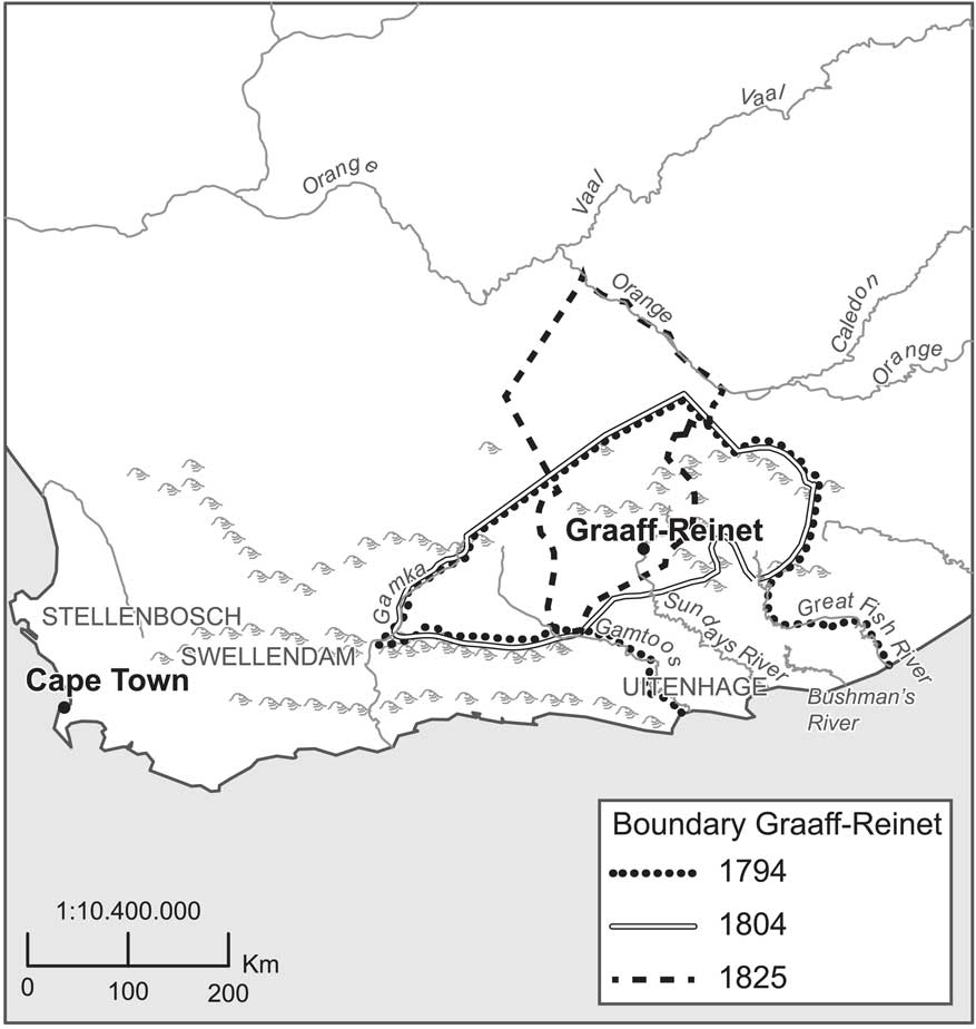
Figure 1 The Graaff-Reinet district expansion from 1795 to 1825.
Some doubt has been cast on whether it truly was this easy for poor frontiersmen to set up as productive stock farmers;Footnote 20 nevertheless, the steady inflow of new settlers to the district continued into the nineteenth century and the best grazing lands were quickly snatched up. A farm of some 6,000 acres could be acquired under the land grant system with relative ease.
The extent to which frontier households were isolated and independent from trade with the domestic market has been the subject of some debate in the South African historiography. While some paint an image of a wayward, solitary, semi-nomadic, and self-sufficient brand of frontiersman,Footnote 21 others maintain that households on the frontier remained relatively orthodox and geared towards production for the market in order to provide for their daily needs.Footnote 22 While scattered evidence of the former can be found, the consensus is that although these households were able to meet some of their basic needs themselves, they were “never entirely cut off from the exchange economy of the south-western Cape”.Footnote 23 On the inhabitants of the Graaff-Reinet district, it has been remarked that “highlights in the lives of the stock farmers were occasional treks to Cape Town, to pay their recognition fees, to marry, to baptize children, to obtain provisions, to redeem their bills. On such occasions the BoersFootnote 24 took cattle with them to sell in Cape Town, and commodities such as butter and soap”.Footnote 25 Indeed, Guelke acknowledges that the expansion of this group of frontier famers could not have taken place without “guns, gunpowder, wagons and other manufactured items obtainable only in exchange for the produce of the interior”.Footnote 26
While the long distance to major markets in the southwestern Cape limited the degree of commercialization, the sale of cattle and sheep still constituted the main source of cash income.Footnote 27 One contemporary traveller, a German doctor of medicine and philosophy, formerly in the Dutch service at the Cape of Good Hope, Henry Lichtenstein, wrote optimistically on large profits to be had from stock farming in this region. He remarked that sheep in this district were favoured above all others in the colony for their weightiness and flavoursome meat. He estimated that “some farmers [had] flocks to the amount of six or seven thousand”. Cows here reportedly “gave richer milk than elsewhere, and in greater abundance” with butter “carried in great quantities to Cape Town, where it [was] always eagerly bought up”.Footnote 28
Allowing for vegetative and seasonal differences, it has been estimated that one sheep or goat required roughly four acres of grazing land, whereas one horse or head of cattle required some eighty acres – a fact that likely contributed to the prevalence of small stock over cattle holding in the frontier districts.Footnote 29 While sheep farming is relatively non-labour intensive compared to crop farming, this was less true in the nineteenth century. Shepherds played an invaluable role at a time before fencing was a mainstay and amidst the ever-present threat of predation or theft by Khoisan raiders. Daily kraaling Footnote 30 meant that each flock of a few hundred heads required a dedicated shepherd.Footnote 31
Where land was to be had on the frontier, ownership was almost exclusively conferred in accordance with the loan farm system, which offered temporary land-use permits in exchange for annual rents.Footnote 32 There is little evidence to suggest that this system created inherent insecurity, since it conferred tenants with exclusive rights to their fixed plot of land. In addition to permits being indefinitely renewable, settlers were free to farm their land without any restrictions or fear of interference from governing authorities. Moreover, applications for licences and permits were seldom refused. Smith notes that “while the Company did not legally surrender its right to take back a loan farm, this was so seldom done that the Boers came to accept that the farms were their own, until they decided to leave; even the failure to pay recognition fees did not result in the revocation of a permit”.Footnote 33
While the land could not technically be sold, settlers could transfer the improvements, resulting in a system of de facto permanent property rights.Footnote 34 In contrast with the visible “affluence and prosperity” of many farmers in the southwestern Cape,Footnote 35 a salient feature of life on the frontier was the high proportion of virtually impoverished farmers.Footnote 36 That is not to say that a small “landed gentry” did not exist, but the majority of pastoral farmers of the frontier it seems, struggled to make ends meet.Footnote 37
Labour demands on the frontier were always high and in times of acute labour shortage, “all who could be exploited as labourers, were exploited”.Footnote 38 This was true for many colonial economies in Africa,Footnote 39 where the incorporation of native and child labour, both free and unfree, kin and non-kin, was viewed as a necessary and acceptable means of meeting domestic production needs, as well as to supply the ever-expanding European market.Footnote 40
There were three main sources of labour available to the frontier farmer: family, slave, and indigenous Khoisan. The importation of slaves to the colony began in 1658, but only flourished at the beginning of the eighteenth century. By 1793, there were 14,747 slaves in the colony compared to 13,830 Europeans.Footnote 41 Unlike the wine and wheat farmers of the regions closest to Cape Town, frontier stock farmers kept comparatively few slaves and while many carried with them the attitudes of a slave holding community, most could only afford to keep one or two.Footnote 42 The average number of slaves per household calculated from the Graaff-Reinet Opgaafrollen for the period 1798–1828 is 1.2 (see Figure 2). This closely matches the traveller John Barrow’s contemporary reckoning that in the district of Graaff-Reinet, in the last decade of the eighteenth century, there were no more than six or seven hundred slaves; approximately one to each family. Moreover, a detailed return for the field cornets office of Op Sneeuwberg (a sub-district of Graaff-Reinet) for 1808, suggests, too, that the distribution of slaves was highly uneven, and that most of the 197 slaves present in that year were concentrated in the hands of the wealthiest inhabitants.Footnote 43 Before 1806, when the British banned the importation of slaves, farmers could have bought newly arrived slaves at the slave auctions in Cape Town. Others may have purchased slaves from other farmers the commercial centre of the southwestern Cape and occasionally non slave-owners may have hired slaves from the large slaveholders, as happened in the southwestern Cape.Footnote 44 But Lichtenstein recalls a passage from the journal of a friend, who, during his visit to the Graaff-Reinet home of “one of the most substantial men the country”, described that the situation of the slaves was “truly lamentable, for he [the farmer] only brought such from Cape Town as were to be purchased at a very cheap rate”.Footnote 45 Barrow noted, too, that Boers preferred the Khoe as labourers because slaves were too expensive.Footnote 46 Indeed, according to the Opgaafrollen, indigenous Khoisan made up the majority of the agricultural labour force on the eastern frontier (see Figure 2).Footnote 47 Note that the Khoisan we are able to capture in our data are limited to those working on European farms. The true population was likely far greater, as some Khoisan were employed by the colonial government, while others managed to survive as independent pastoralists.
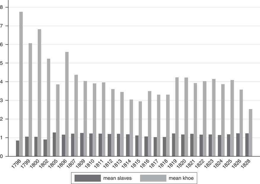
Figure 2 Mean number of slaves and Khoe employed on settler farms annually, 1798–1828.
Lack of reliable information on the latter prevent us from making even an educated guess regarding the size of the total Khoisan population in the district. Some Khosian will have been residing in the district prior to the arrival of the Europeans, while some may have had originated from the northern and southwestern Cape and accompanied the Europeans as they moved into the interior, working for them as interpreters, carriers, and domestic servants. The Khoisan residing on the European farms consisted of captured runaways (who had joined the Xhosa fighting against further European expansion), apprentices, and “free” men, who, having lost their kraals were left with no other choice than to work for Europeans.Footnote 48 The latter group was the most important source of non-family labour in the district, reportedly often living in dismal conditions on their employers’s farms. Traveller John Campell recalled in 1822 that the conditions for some Khoe labourers were often worse than that of the slaves.Footnote 49 However, the daily lives and circumstances of these two groups cannot be thought of as distinct from one another. As Mason argues:
Slaves lived and worked beside these servants, performing the same tasks – shepherd, cattleherd, field labourer, household servant, and sometimes overseer – and experiencing the same forms of labour control, which was a blend of coercion and incentive [with farmers adopting] a style of labour relations which had indeed blurred the lines between slavery and other forms of labour subjugation.Footnote 50
We are therefore careful not to treat slaves and Khoisan labour as two separate groups of free and non-free labour, but rather as a combined group, distinct from so-called family-labour.Footnote 51
THE CLOSING OF THE GRAAFF-REINET FRONTIER
The period under investigation in this paper was characterized by major political and institutional change. Initial European expansion into the eastern frontier was followed by decades of instability and hostility between the Europeans, the indigenous Khoisan, and the Xhosa tribes. The expansion of the European settlement on the eastern frontier made it increasingly difficult for the Khoisan to survive as independent pastoral farmers. As early as 1773, Governor Van Plettenberg wrote that in Graaff-Reinet “[…] there are no Hottentots except those who since several years had hired themselves to the colonists”.Footnote 52 This was likely an exaggeration; nonetheless, in 1775, in an attempt to further tighten European control over Khoisan labour, the VOC formally instituted the Inboekstelsel – a pass system that severely inhibited the movement of Khoe who did not carry papers showing that they were employed.
Some Khoisan groups resisted European expansion with success. In 1785, Khoisan had successfully regained control over the land in Sneeuburgen in the north and Camdeboo in the west of Graaf-Reinet, but their success was short-lived.Footnote 53 Instability deepened due to political uncertainty following the decline of the Company and the first British occupation (1795–1802). Countless episodes of violence and conflict littering the final decade of the eighteenth century (indicative of the continued dissatisfaction amongst the Khoe with their former dispossession at the hands of the Boers)Footnote 54 together with mounting dissatisfaction with their working conditions, culminated in the so-called Bushman Wars (1799–1802), which saw an alliance between Xhosa chiefs and Khoe rebels temporarily cripple the frontier economy and dispel many Boers from their farms.Footnote 55
In the early nineteenth century, the English made further attempts to formalize indigenous subjugation through indenturing Khoe labour to European settler farmers by implementing the Caledon Code of 1809. It allowed European farmers to keep children of slave fathers and Khoe mothers on their farms until they reached the age of twenty-five.Footnote 56 While the tension between the Europeans and the indigenous populations never completely eroded, the situation gradually stabilized after the second British occupation.Footnote 57 By the end of our period of investigation, European settlers had regained control over most of the desirable land in the district, though some Khoisan were permitted grazing rights European controlled land.Footnote 58
The British takeover of the Cape Colony also resulted in a major exogenous shock to the settler population, not least due to the arrival of some 4,000 British settlers to the eastern parts of the Colony, but perhaps more importantly with the ban of slave importation in 1808.Footnote 59 While the use of slaves was not as widespread in the Graaff-Reinet district as it was in the southwestern Cape, there is evidence suggesting that frontier farmers were nevertheless affected by the increased prices of slaves and the resulting increase in wages for Khoisan labourers.Footnote 60
These changes took place in parallel to the closing of the frontier, in both an economic and administrative sense. Administratively, the establishment of the Uitenhage district in 1804 effectively closed the southern border of Graaff-ReinetFootnote 61 leaving only the northern border open. More importantly, the availability of land was substantially reduced during the period of investigation. We lack systematically recorded data to quantify the closing, but all qualitative evidence suggests that, although land was initially cheap and plentiful, settlers, particularly those with expanding flocks, soon found sufficient grazing lands more difficult obtain. By 1812, only thirty-nine per cent of married men owned their own farm, and there were no independent Khoisan settlements left in the district.Footnote 62 This does not mean that there was a large group of landless Boers, as many occupied land illegally or rented land from relatives or friends.Footnote 63 Still, the possibility of accessing land cheaply was becoming more limited and, in 1813, the loan farm system was replaced by the quitrent system. Coupled with ineffectual administration, the processing of new land claims became increasingly protracted.
In 1824, the district boundaries were officially extended beyond the Orange River to meet the “insatiable need of an ever-increasing population for more land”.Footnote 64 Increased population pressure further limited access to grazing lands with sufficient water supply. In 1826, the Landrost of Graaff-Reinet, Stockenstrom concluded that, “[...] when we speak of occupation, there is not even a stagnant pool that keeps rain water for any length of time which is not regularly occupied, so that of course no spring remains vacant”.Footnote 65
The frontier was never entirely closed. Instead, the increased population pressure and shrinking land availability led to the well documented Great Trek of 1834–1838, as trekboers crossed the Orange River and moved further into the northeast of present day South Africa.Footnote 66
DATA AND METHODS
Until recently, most research on historical household formation in South Africa has been anecdotal, either coming from traveller accounts, or based on records that are subject to selection problems.Footnote 67 New research offers a more comprehensive account of the settler fertility transition beginning in the second half of the nineteenth century.Footnote 68 But very little is known about pre-transitional household composition in this society and geographically disaggregated micro-level data are needed to better understand the demand for children on frontier farms and how it differed across socio-economic strata.
We combine two newly transcribed datasets. The first is the Opgaafrollen: annual tax censuses collected between 1663 and 1834 by the Dutch East India administration, and after 1795, by the British colonial administration, of all free households of the Colony. Household-level information includes name and surname of the head of the household and spouse, the number of children present in the household, the number of slaves and indigenous Khoisan employed, and several agricultural inputs and outputs, including cattle, sheep, horses, wheat sown, wheat reaped, vines, and wine produced. All males over the age of sixteen were assessed for tax purposes. Unless they headed a household, females were not included. The full series of Opgaafrollen are in the process of being transcribed and the household contained therein, identified and linked across years using a probabilistic record linkage strategy to create an annual panel of household production across more than a century.Footnote 69
We use a sub-sample of these censuses for the Graaff-Reinet district covering the period 1798–1828. The panel contains 35,199 observations over twenty-eight years,Footnote 70 comprised of 10,162 unique households. But, since these data do not contain information on birth dates (crucial in controlling for, and distinguish between, age, period, and cohort effects) or death dates (crucial for controlling for lifecycle wealth effects), we supplement these data with individual-level demographic data for the household head from the South African Families Database (SAF). Obtained from the Genealogical Institute of South Africa (GISA), these data contain information on all settler families from 1652 to approximately 1830 as well as those of new progenitors of settler families up to 1867. The probabilistic record linkage strategy that was used to identify and match households over time to create the CGHP is applied to identify and match heads of households across these two sources with a match rate of between 40 and 60 percent annually.Footnote 71
Information on household assets and production in the Opgaafrollen was used to estimate household wealth.Footnote 72 We choose to estimate separately what we will henceforth refer to as “asset wealth” and “capital wealth”. We take the asset component of wealth as the total real value of livestock, by multiplying the number of small livestock (sheep, cattle and goats) owned in a given census year by the estimated value thereof using a series of livestock prices from probate inventories (MOOC 8 Series, TANAP 2012).Footnote 73 In order to determine the capital component of wealth, we sum all productive assets owned by an individual in a given census year.Footnote 74 Through the selection of variables, we have tried to identify those elements necessary to capture improved capacity to produce a surplus for the market. These include number of horse wagons, horses, oxen, ox wagons and carts.Footnote 75
RESULTS
It is useful to begin with an examination of the typical household structure and economic circumstances of the population in question. Table 1 shows the characteristics of an average farming household in our population. On average, frontier farms housed two adult settlers (typically a husband and a wife), and two settler children in a given census year. We can see that rearing stock was clearly the dominant economic activity on frontier farms, with the average farm accommodating over 500 heads of sheep and around fifty heads of cattle.
Table 1 Characteristics of frontier farms.
Notes: Grains sown in a given year are reported in muids, a South African measure of dry capacity equivalent to about 109 litres.
It has been suggested, however, that a man with just fifty sheep or thirty cattle would not have been in a position to support himself, let alone his family.Footnote 76 If we consider the proportion of households owning less than fifty sheep or thirty cattle in a given year, shown in Figures 3 and 4, we can indeed see that many stock famers were barely making ends meet. It is also important to the degree of variation in both sheep and cattle ownership; one particularly wealthy farmer owned some 12,000 heads of sheep, while another had 2,813 heads of cattle in a given year. But these extremely wealthy individuals appear to be a minority. On average, households owned around six horses and nine oxen, sufficient to pull their carts and wagons to market and to drive their ploughs. Graaff-Reinet was not known for being a grain-producing district, which is evidenced by the low volume of wheat, barley, oats, and rye sown in any given year. That is not to say that farmers did not engage in these activities, if only for subsistence.
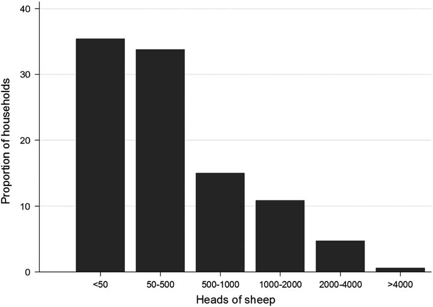
Figure 3 Proportion of settler households owning sheep, Graaff-Reinet district, 1798–1828.
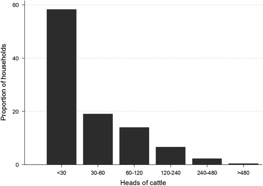
Figure 4 Proportion of households owning cattle, Graaff-Reinet district, 1798–1828.
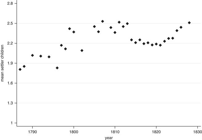
From Figure 5, we can see that the average number of settler children in frontier households steadily increased over the period of frontier closure in Graaff-Reinet. From Figure 6, we can see that the presence of children in frontier households has a clearly positive association with wealth if we consider this population across wealth quintiles, before taking into account any variation over time.
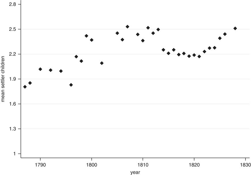
Figure 5 Average number of settler children present in settler households, Graaff-Reinet district, 1798–1828.
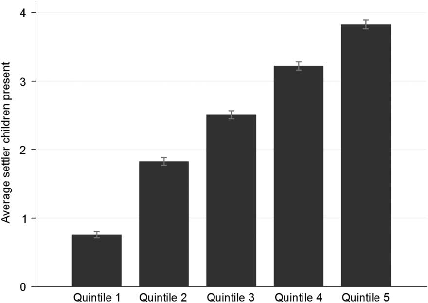
Figure 6 Average number of settler children present in settler households by real wealth quintile, Graaff-Reinet district, 1798–1828. Notes: The number of observations in quintiles 1–5 are 7693, 6546, 6900, 7042, and 7018 respectively.
Given the large variation in livestock and capital holdings described it is critical that we account for the high degree of inequality in this society. We begin by estimating a Gini coefficient for every year in our panel, the results of which are shown in Figure 7. In line with findings for the Cape Colony in general,Footnote 77 these results confirm that the farming population of Graaff-Reinet was indeed highly unequal, with the Gini coefficient consistently above 0.6.
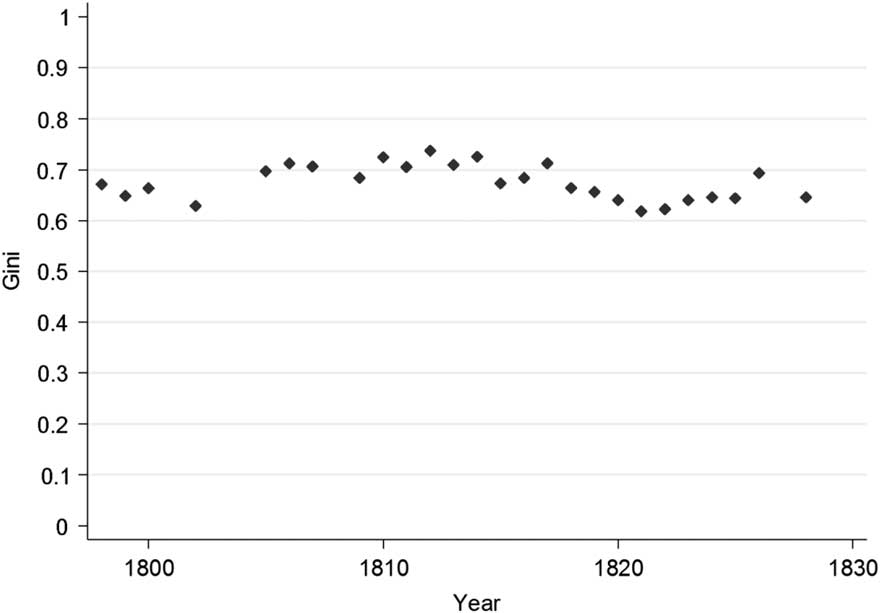
Figure 7 Annual Gini coefficient, Graaff-Reinet district, 1798–1828.
Further evidence of a small but very wealthy elite is presented in Figure 8, which shows that the average total value of assets owned by the wealthiest five per cent was ten times more than the rest of the population. Returning, then, to the relationship between wealth and family size, we find that the wealthiest five per cent had a family size sixty per cent larger than the remaining ninety-five per cent of the population, as shown in Figure 9.
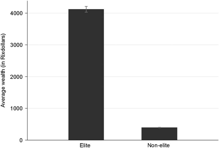
Figure 8 Average real wealth (in Rixdollars) for the elite (wealthiest top 5 per cent of the sample) versus non-elite (bottom 95 per cent of the sample), with 95 per cent confidence bars.
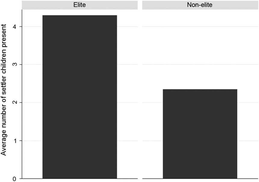
Figure 9 Average number of settler children present in the households of the elite (wealthiest top 5 per cent of the sample) versus the non-elite (bottom 95 per cent of the sample).
It is critical, therefore, to take into account these stark societal inequalities when characterizing economic and social behaviour over time. We are able to control for this variation in wealth using a simple regression framework in which we estimate the association between capital and livestock wealth, non-family labour, and settler children present for all households over time.Footnote 78 Figure 10 summarizes the coefficients from our first model, which has as the dependent variable, the number of settler children present in a household. We find a positive association between livestock wealth, capital wealth, and the presence of non-family labourers in the household, respectively, with the presence of settler children in frontier households.Footnote 79
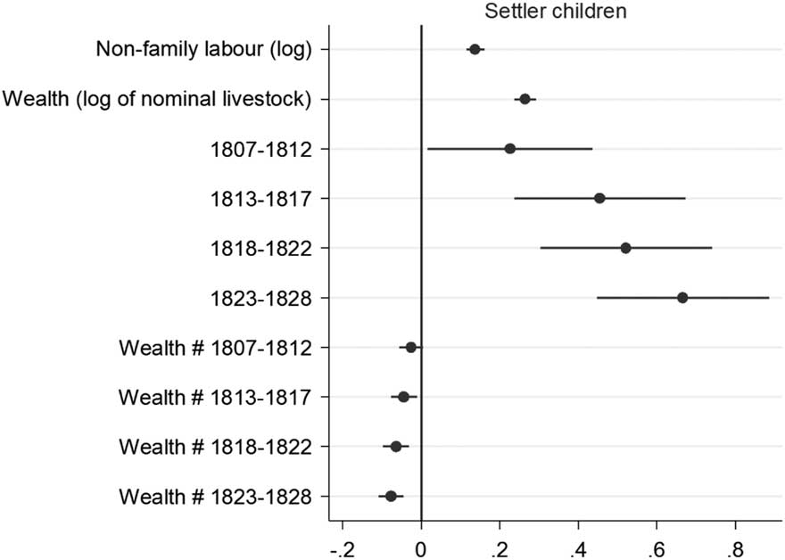
Figure 10 Summary of coefficients from a negative binomial regression with dependent variable: settler children. Notes: All coefficients were significant at the 95 per cent level. Figure corresponds to model 2 in Table A1.
We also want to establish how this relationship changed over time in order to determine the effect of a closing frontier. We find that, over time, the presence of settler children in frontier households is negatively associated with wealth, i.e. while in absolute terms the wealthiest households report more settler children present, they begin to reduce this over time. This reduction could be the result of conscious fertility limitation within this group, or a feature of higher social mobility for the children of wealthy farmers, i.e. children of the wealthy may have been more likely to pursue opportunities outside the family farm.
However, the strong positive association of wealth (in its various forms) and children present might be explained if there is a high correlation between asset wealth and the age of the household head, if we believe that individuals typically accumulate assets and children over the course of their lives. Using a sub-sample of households matched to the SAF database, for which we can determine the age of the head of the household, we can deduce whether such effects are present as well as control for them in our models. From figures 11, 12, and 13, we can clearly see that there are strong lifecycle effects with respect to wealth and children.
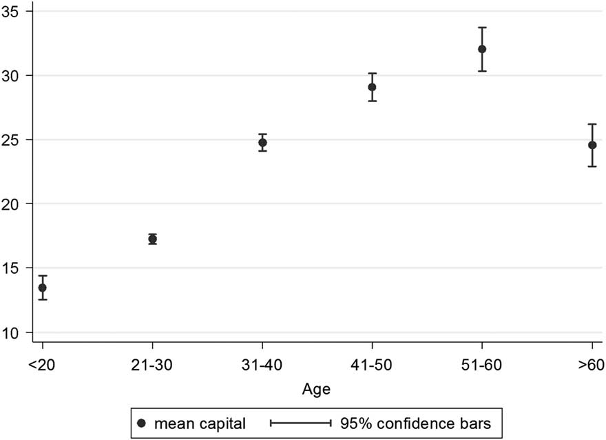
Figure 11 Mean capital by household head age, with 95 per cent confidence bars.
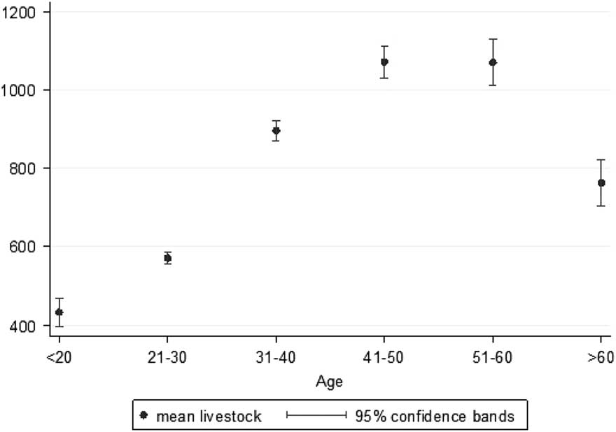
Figure 12 Mean wealth (livestock) by household head age, with 95 per cent confidence bars.
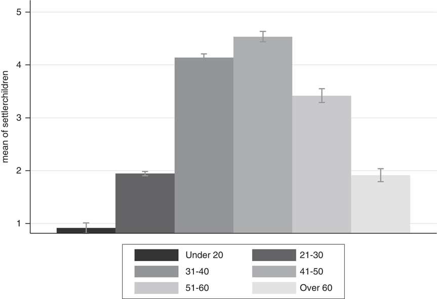
Figure 13 Mean settler children by household head age, with 95 per cent confidence bars.
Note that, since the size of the linked sample is much smaller than the full sample, resulting from the fact that not all household heads were able to be identified and matched to the genealogical registers, we limit the use of the linked sample to checks on model robustness. However, even with reduced sample size, the magnitude and significance of the coefficients of interest remain, i.e. controlling for the positive effects of the age of the household head on the number of children present and overall household wealth, an independent positive correlation between livestock wealth, capital wealth, and the presence of slave and Khoe labour remain significant.
Next, we want to see how different wealth groups substitute between family and non-family labour. For this, we consider the ratio of children to non-family labour (slaves plus Khoe) present on the farm in a given census year. A higher ratio is indicative of more non-family labour being employed relative to family labour. Figure 14 summarizes the results of our model, which shows a positive association of both capital wealth and livestock wealth with the use of non-family labour, suggesting that wealthier households could indeed afford to own more slaves and employ more Khoe than poorer households. We can also see that the use of non-family labour was declining over time. The reduction in the ratio of family to non-family labour over time for the wealthy is also larger than for the poor, due to the fact that while the use of both family and non-family labour was decreasing for this group, the relative decline of non-family labour was larger.
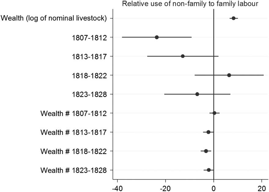
Figure 14 Summary of coefficients from an ordinary least squares regression with dependent variable: family to non-family labour ratio. Notes: Figure corresponds to model 4 in Table A1.
But if we believe that frontier households desired to maintain output amidst frontier closure, we ought to question why the wealthy chose to reduce both family and non-family labour. We therefore consider the ratio of capital to labour over time – a larger ratio being indicative of relative capital intensification. From Figure 15, we can see that for the population in general, we find evidence that the wealthy remained more labour intensive than the poor in absolute terms, but that, over time, chose to invest in more carts, wagons, oxen, horses, and breeding animals so as to allow themselves greater productive capacity and better market access relative to labour, to a greater extent than the poor.
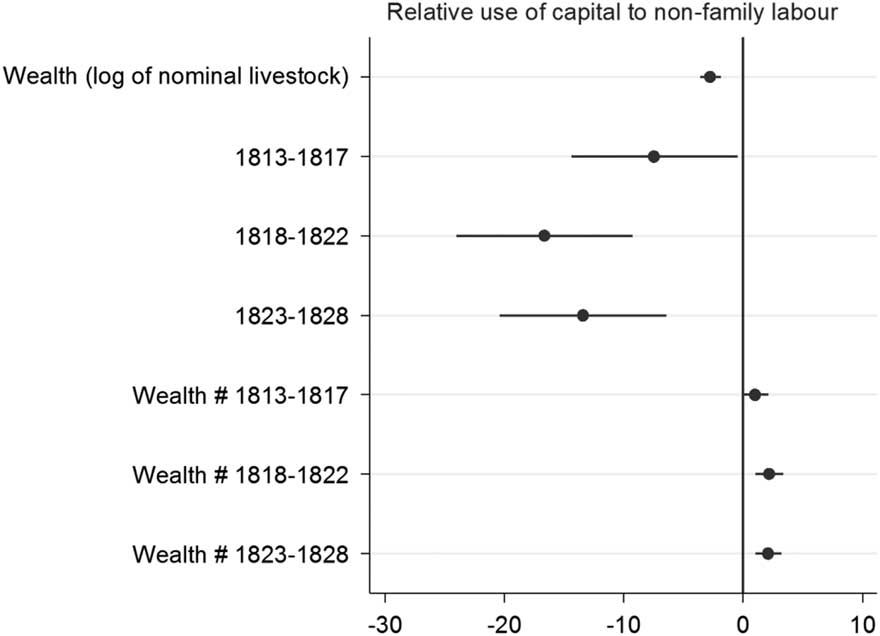
Figure 15 Summary of coefficients from an ordinary least squares regression with dependent variable: capital to labour ratio. Notes: Figure corresponds to model 6 in Table A1.
CONCLUDING DISCUSSION
Since the 1960s, studies have found that fertility declines in the nineteenth-century Western world cannot be fully understood without considering the population dynamics in the rural areas. Focusing on the rural US and Canada, scholars found that fertility levels systematically differed between newly established frontier regions and older ones. Fertility levels were significantly lower in the established and more densely populated areas compared to the less densely populated frontier regions. Although a lack of data prevents more precise empirical testing, these systematic differences in fertility levels have commonly been explained by the land–labour hypothesis. Fertility levels were higher in frontier regions either because the demand for child labour was larger and/or the cost of having children was lower.
In this paper, we contribute to the debate by analysing the relationship between land availability and children present in settler farming households in the Graaff-Reinet district at the eastern frontier of Cape Colony. Different from the frontier literature, we find for the Graaff-Reient district that the closing of the frontier was associated with an increased presence of children.
We identify two weaknesses in the frontier literature: the failure to account for wealth inequalities and the failure to distinguish between family and non-family labour. Rural populations will respond differently to shrinking land availability depending on their wealth because the latter determines the available adaption strategies. A rich farm household may respond to diminishing land availability by substituting labour for capital, while this option is simply not available to a poor household. Wealth inequality in Graaff-Reinet was considerable and the vast majority of frontier farmers struggled to subsist. So, while a small minority did indeed respond to shrinking land availability by developing more capital-intensive methods of production, the poor did not. We find that the poorer farmers responded by increasing their relative use of family labour. This strategy makes economic sense if we – different from the frontier literature – make a clear distinction between family and non-family labour. The employment of non-family labour is dependent on the marginal productivity of labour. This is not the case for family labour as shown by development economists, agrarian historians, and economic historians. On the contrary, in pre-industrial societies, farmers will respond to shrinking land availability by adding more labour to land despite decreasing marginal productivity of labour. This Boserupian path was what the majority of the Graaff-Reinet population followed. Lacking alternative means to using family labour, they intensified labour use in light of shrinking land availability, which created a demand for having more children.
This leads us to conclude that, for the poor, we see a negative correlation between land availability and labour demand. The reason why the Graaff-Reinet households experienced, on average, an increased presence of settler children in the midst of a closing frontier, is that a large majority of the population consisted of the poor. In that regard, our study does not necessarily contradict previous findings. It may very well be that farmers in nineteenth-century US and Canada were, on average, wealthy enough to respond to shrinking land availability by employing more capital intensive farming methods. The implications of our findings are, however, that the positive relationship between fertility and land availability may not be universal, as previously thought, but largely dependent on levels and distribution of wealth among the rural inhabitants.
EMPIRICAL APPENDIX
To model the effects of wealth and the use of non-family labour on the presence of settler children in frontier households, negative binomial distribution models were selected over ordinary least-squares as they are designed to analyse count data and account for the fact that the number of children in a family is non-negative. They also account for over-dispersion (where the mean is greater than the variance) common in fertility data, by treating dispersion as a parameter to be estimated from the data.Footnote 80 Over-dispersion in our sample results from excess zeros, due to many households being observed before childbearing begins. We run the following specification:
 $$y_{{it}} \,{\equals}\,\alpha {\plus}\beta _{1} \,{\rm ln}(Labour_{{it}} ){\plus}\beta _{2} \,{\rm ln}(Wealth_{{it}} ){\rm }{\plus}\beta _{3} (Period){\plus}{\epsilon}_{{it}} $$
where y it is the number of settler children present in household i in year t. β 1, and β 2represent the effects of the log of non-family labour, and nominal livestock wealth, respectively, and are our outcome variables of interest. β 3 represents the effects of the categorical variables representing five time periods from 1789-1828. ε it represents unobservable determinants that vary across time and individuals. We cluster at the household level to obtain robust standard errors.
In specification 2, wealth and period are interacted to model the effect over time:
 $$\eqalignno{ y_{{it}} \,{\equals}\,&\alpha {\plus}\beta _{1} \,{\rm ln}\left( {Labour_{{it}} } \right){\plus}\beta _{2} \,{\rm ln}\left( {Wealth_{{it}} } \right) {\plus}\beta _{3} \left( {Period} \right)\cr & {\plus}\beta _{4} (\ln \left( {Wealth} \right)_{{it}} {\rm {\asterisk}}Period){\plus}{\rm }{\epsilon}_{{it}} $$
To model the relative use of non-family labour in frontier households, we use OLS with the following specification:
 $${{y_{{it}} } \over {L_{{it}} }}\, {\equals}\, \alpha {\plus}\beta _{1} \,{\rm ln}(Wealth_{{it}} ){\plus}\beta _{2} (Period){\plus}{\epsilon}_{{it}} $$
Where
 ${{y_{{it}} } \over {L_{{it}} }}$
represents the ratio of family to non-family labour in household i in year t. To account for the fact that such a ratio may be unstable if the denominators are small, or indeterminate if the denominators are ever 0, we use instead, the following expression to summarize the relative change of non-family labour with respect to family labour:Footnote
81
${{y_{{it}} } \over {L_{{it}} }}$
represents the ratio of family to non-family labour in household i in year t. To account for the fact that such a ratio may be unstable if the denominators are small, or indeterminate if the denominators are ever 0, we use instead, the following expression to summarize the relative change of non-family labour with respect to family labour:Footnote
81
 $$100{\asterisk}((y_{{it}} \,/\,(y_{{it}} {\plus}L_{{it}} )){\minus}(L_{{it}} \,/\,(y_{{it}} {\plus}L_{{it}} )))$$
β 1 represents the effects of the log of livestock wealth and is again our main variable of interest. In specification 4, wealth and period are again interacted to model the effect over time:
 $${{y_{{it}} } \over {L_{{it}} }}\, {\equals}\, \alpha {\plus}\beta _{1} \,{\rm ln}(Wealth_{{it}} ){\plus}\beta _{2} \left( {Period} \right){\plus}\beta _{3} ({\rm ln}(Wealth)_{{it}} {\rm {\asterisk} }Period){\plus}{\epsilon}_{{it}} $$
Lastly, to model relative labour and capital intensification as it relates to household wealth we use OLS with the following specification:
 $${{L_{{it}} } \over {C_{{it}} }}\, {\equals}\, \beta _{1} \,{\rm ln}(Wealth_{{it}} ){\rm }{\plus}\beta _{2} \left( {Period} \right){\plus}{\epsilon}_{{it}} $$
Where
 ${{L_{{it}} } \over {C_{{it}} }}$
represents the ratio of labour to capital in household i in year t, again estimated as:
${{L_{{it}} } \over {C_{{it}} }}$
represents the ratio of labour to capital in household i in year t, again estimated as:
 $$100{\asterisk}((L_{{it}} \,/\,(L_{{it}} {\plus}C_{{it}} )){\minus}(C_{{it}} \,/\,(L_{{it}} {\plus}C_{{it}} )))$$
In specification 6, wealth and period are again interacted to model the effect over time:
 $${{L_{{it}} } \over {C_{{it}} }}\, {\equals}\, \beta _{1} \,{\rm ln}(Wealth_{{it}} ){\plus}\beta _{2} \left( {Period} \right){\plus}\beta _{3} ({\rm ln}(Wealth)_{{it}} {\rm {\asterisk} }Period){\plus}{\epsilon}_{{it}} $$
For the SAF linked sample we following the same specification as equation (1), with the inclusion of θ and Φ which represents the potentially non-linear effects of age (a it ) and age squared (a it )2
 $$\eqalignno{ y_{{it}} {\equals}& \alpha {\plus}\beta _{1} \,{\rm ln}\left( {Labour_{{it}} } \right){\plus}\beta _{2} \,{\rm ln}\left( {Wealth_{{it}} } \right) {\plus}\beta _{3} \left( {Period} \right) \cr & {\plus}\beta _{4} ({\rm ln}(Wealth)_{{it}} {\rm {\asterisk} }Period){\plus}\theta \left( {a_{{it}} } \right){\plus}{\rm \Phi }\left( {a_{{it}} ^{2} } \right){\plus}{\epsilon}_{{it}} $$
Table A1 Estimates from negative binomial and OLS models.
Table A2 Estimates from linked sub-sample negative binomial regressions.