On the Analytical and Numerical Solutions of the Linear Damped NLSE for Modeling Dissipative Freak Waves and Breathers in Nonlinear and Dispersive Mediums: An Application to a Pair-Ion Plasma

1 Introduction

In the past few years, interest has increased in the treatment required to solve differential equations analytically and numerically which led to the interpretation of ambiguous nonlinear phenomena that exist and propagate in various fields of science such as the field of optical fiber, Bose-Einstein condensate, biophysics, Ocean, physics of plasmas, etc. [1–19]. For instance, the Schrödinger-type equation and its family are devoted to interpreting and investigating the behavior of waves accompanied by the movement of particles in multimedia [4–20]. Additionally, the family of the nonlinear Schrödinger-type equation is used to investigate modulated envelope structures such as dark solitons, bright solitons, gray solitons, rogue waves, breathers structures etc. which can propagate with group wave velocity [11–20]. This family has been solved analytically and numerically using several analytical and numerical methods [1]. The following standard/cubic NLSE

is considered one of the most universal models used to describe and interpret various physical nonlinear phenomena that can exist and propagate in nonlinear and dispersive media. Numerous monographs and published papers are devoted to studying the NLSE which possesses a special solution in the form of pulses, which retain their shapes and velocities after interacting among themselves. Such a solution is called modulated envelope dark soliton. Other nonlinear modulated structures such as bright and gray solitons, cnoidal waves, etc. could be modeled using Eq. 1 and its family. Furthermore, the importance of Eq. 1 extends to the explanation of some mysterious modulated unstable phenomena such as rogue waves (RWs)/freak waves (FWs)/killer waves/huge waves/rogons, all names are synonymous. These waves were observed for the first time in ocean and marine engineering [21] and then extended to appear in many branches of science such as in water tanks [18, 22], finance [23], optical fibers [24–26], in atmosphere and astrophysics [27, 28], and in electronegative plasmas [29–32], etc. In recent decades, explaining the mechanisms of rogue wave (RW) propagation in different systems have been one of the main topics that occupy the minds of many researchers.

RWs have been described by many researchers as temporary/instantaneous waves “that appear suddenly and abruptly disappear without a trace” [33]. RWs possess some characteristics that distinguish them from other modulated waves such as, 1) it is a space-time localized wave i.e., not periodic in both space and time 2) it is a single wave which propagates with the largest amplitude compared to the surrounding waves (almost three times [29] (for first-order RWs) or five times [31] (for second-order RWs), and 3) the statistical distribution of the RW amplitude has a tail that does not follow the Gaussian distribution [34]. Furthermore, there is another type of unstable modulated structure that can be described and investigated by Eq. 1 and its family, which are called the solitons on finite backgrounds (SFB) or are known as breathers waves including the Akhmediev breathers (ABs) and the Kuznetsov–Ma breathers (KMBs) [35]. Both the ABs and the KMBs are exact periodic solutions to Eq. 1. With respect to the ABs and according to Eq. 1, it is a space-periodic solution but is localized in the time domain. On the contrary, with respect to the KMBs, it is a time-periodic solution but is localized in the space domain. Both the ABs and KMBs have a plane wave solution when $\left|t\right|\to \infty$ and $\left|x\right|\to \infty$, respectively. Furthermore, for a limiting case of the periodic breathers, both the ABs and KMBs become localized (i.e., the ABs and KMBs become RWs) in the temporary and spatial domain, [36, 37].

To understand and interpret the puzzle of generating and propagating these types of huge waves in various fields of sciences, many researchers focused their efforts to solve the integrable NLSE and its higher-orders, which describe the analytical RWs and breathers solutions. Most published papers about these waves have been confined to investigating the undamped RWs and breathers in the absence of the damping forces (the friction force or collisions between the media particles) [19, 38–40]. In fact, we can only neglect the force of friction in very few cases of superfluids (no viscosity). So consequently, this force must be taken into consideration when studying the propagation of these waves in optical fiber, laser, physics of plasmas, etc. to ensure the phenomenon under consideration is described accurately and comprehensively. Recently, different experimental approaches have been used to generate the dissipative RWs (DRWs) in Mode-Locked Laser [41], multiple-pulsing mode-locked fiber laser [42], fiber laser [43], and in an ultrafast fiber laser [44]. Theoretically, few attempts have been made to understand the physical mechanism of generating and propagating DRWs and DBs (dissipative Akhmediev breathers (DABs) and dissipative Kuznetsov-Ma breathers (DKMBs) in the fluid mechanics and in plasma physics when considering the friction forces [45–50]. In these papers, authors tried to find an approximate analytical solution to the following non-integrable linear damped NLSE.

These studies relied on the use of an appropriate transformation [45] to convert Eq. 2 into the integrable NLSE (1) which has a hierarchy of exact analytical solutions such as envelope solitons, RWs, breathers, cnoidal waves, etc. Motivated by the observations of RWs in the laboratory in the case of electronegative plasmas and a fiber laser, we have made some subtle and distinguishable attempts to obtain some approximate analytical and numerical solutions for Eq. 2 without converting this equation to the standard cubic NLSE (1). In the first attempt (our first objective), the DRWs and DBs solutions will be obtained in the form of semi-analytical solutions based on the exact analytical solution to Eq. 1. To our knowledge, this is the first attempt to derive an approximate analytical solution with high accuracy for the DRWs and DBs of Eq. 2 without transforming it to Eq. 1. The second objective of our study, is to use some hybrid numerical methods, such as the moving boundary method (MBM) with the finite difference method (FDM), to solve the non-integrable Eq. 2 numerically and to make a comparison between the numerical approximate solution and the semi-analytical solution to check the accuracy and the effectiveness of both of them. Moreover, the maximum local (at a certain value of time, say, at final time) and global (taken over all space-time domain) errors of the semi-analytical solution are estimated. Furthermore, the error functions related to the whole space-time domain and final time for the semi-analytical solution is evaluated using the polynomial based on the Chebyshev approximation technique. The most important characteristic of our techniques is their ability to give an excellent, accurate, and comprehensive description for the phenomena under study.

The remainder of this paper is structured as follows: in Section 2, we briefly review the results obtained by Sikdar et al. [49] studying both collisionless and collisional envelope solitons in collisional pair-ion unmagnetized plasmas with completely depleted electrons. The profile of modulational instability (MI) of the (un)damped electrostatic potential is also analyzed and investigated in Section 2. Moreover, the (un)stable regions of ion-acoustic (IA) modulated structures are determined precisely, depending on the criteria of the MI of non-dissipative and dissipative modulated structures. In Section 3, the exact analytical RW and breathers solutions to Eq. 1 are discussed briefly. Thereafter, we devote great effort to solve and analyze Eq. 2 analytically to obtain a semi-analytical solution to the DRWs and DBs. In Section 4, the hybrid MBM-FDM is introduced to analyze Eq. 2 to investigate the characteristics behavior of both the DRWs and DBs. The results are summarized in Section 5.

2 The Physical Model and a Linear Damped NLSE

Sikdar et al. [49] reduced the fluid governing equations of the collisional pair-ion unmagnetized plasmas to the linear damped NLSE using a reductive perturbation technique (the derivative expansion method) to study both collisionless and collisional envelope solitons (bright and dark solitons). In this model, the plasma system consists of warm positive and negative fullerene ions ($C_{60}^{+}$ and $C_{60}^{-}$) in addition to considering the ion-neutral collision [49, 51]. The linear damped NLSE obtained by Sikdar et al. [49] is similar to Eq. 2. In Sikdar et al. [49] model, the linear damping term ($iR\text{Ψ}$) appeared as a result of considering the ion-neutral collision. The coefficients P, Q, and R represent the coefficients of the dispersion, nonlinear, and linear damping terms, respectively. These coefficients are functions of various plasma parameters such as, the temperature $T_{\pm }$ and the ion-neutral collision frequency ${\nu }_{\pm }$ of both the positive and negative ions. The derivation details of the linear damped NLSE for the present model and the values of P, Q, and ${\text{Γ}}_c$ can be found in Ref. 49. Sikdar et al. [49] observed that in the dimensional form, the system supports two modes, namely, high frequency ion plasma wave (IPW) and low frequency ion-acoustic wave (IAW). They also observed that for the IPW both P and Q are always positive against the modulated wavenumber (k) and for different values of $\left(T_{+},T_{-}\right)=\left(0.9,0.6\right)$ and $\left(T_{+},T_{-}\right)=\left(\mathrm{0.0.54},0.9\right)$. On the other hand, for the IAW, the coefficient P is always negative while the coefficient Q may be positive or negative depending on the value of the modulated wavenumber. Moreover, it was found that the coefficient of the dissipative term ${\text{Γ}}_c$ is always positive for all cases. It is known that in the absence of the dissipative/damping term (${\text{Γ}}_c=0$), the standard NLSE supports a series of exact analytical solutions like the dark solitons, bight solitons, gray solitons, RWs, breathers (Akhmediev breathers (ABs), and Kuznetsov–Ma breathers (KMBs)), etc. On the contrary, in the presence of the dissipative term (${\text{Γ}}_c\ne 0$), the linear damped NLSE becomes completely non-integrable, i.e., it does not have an exact analytical solution in its present form. As a result, this equation could be solved numerically or semi-analytically by one of the known methods describing many nonlinear modulated structures that can exist and propagate in different branches of science [49].

Without loss of generality, we can rewrite the linear damped NLSE in the following form Refs. 49 and 52.

where $P\equiv P/2$ and ${\text{Γ}}_c\equiv R$.

According to the linear stability analysis and for undamped modulated structures $\left(R=0\right)$, the nonlinear modulated envelope excitations (IWA and IPW) become stable (unstable) if $Q>0(Q<0)$ is fulfilled [53]. In this case, the sign of the product $PQ$ is a necessary and sufficient condition to determine the regions of different types of modulated excitations in the present model. However, for damped modulated structures $\left(R\ne 0\right)$, the criteria for MI of envelope excitations become a function of time in addition to the physical parameters related to the model under consideration and in this case, there are other restrictions on the propagation of the dissipative IAW and IPW envelope structures [46–50, 54, 55]. In this case and according to the linear stability analysis, the value of nonlinear dispersion relation is obtained as: ${\text{Ω}}^2={\left(P{K}^2\right)}^2\left(1-K_c^2\left(\tau \right)/K^2\right)$, with the critical modulated wavenumber $K_c^2\left(\tau \right)=\left(2Q/P\right)|{\psi }_0{|}^2\text{exp}\left(-2R\tau \right)$ where $\text{Ω}\left(\ll \omega \right)$ and $K\left(\ll k\right)$ refer to the perturbation frequency and wavenumber in the slowly coordinates $\left(x,t\right)$, ${\psi }_0$ donates the amplitude of the pumping carrier wave (which is a constant value and larger than the perturbation value). At first glance, we can see that the modulated structures become unstable if $PQ>0$ & ${\text{Ω}}^2<0$ & $t<t_{\text{max}}$ are fulfilled. Here, t donates the time (or period) of the wave propagation and $t_{\text{max}}=\left[1/\left(2R\right)]\text{ln}\left[2Q\right|{\psi }_0{|}^2/\left(P{K}^2\right)\right]$ gives the MI period [46–50]. On the contrary, for $t\mathrm{>}{t}_{\text{max}}$ even if $PQ>0$, the modulated envelope structures become stable and in this case both dissipative RWs and dissipative breathers cannot exist in this model. It can be seen that for $R=0$, the critical wavenumber of modulated structures $K_c^2=\left(2Q/P\right)|{\psi }_0{|}^2$ does not depend on t.

In the present study, we take the IAW mode as an example for applying our numerical and semi-analytical solutions for investigating the behavior of the dissipative RWs and dissipative breathers. Knowing that the analytical and numerical solutions that we obtain can be applied to any system and mode, we only take the IAW mode as an example. The (in)stability regions electrostatic modulated structures must be determined precisely before embarking on solving this equation. Figure 1 demonstrates the (un)stable regions of the (un)damped modulated structures according to the above mentioned criteria. In Figures 1A–C the product of $PQ$, the square perturbation frequency of modulated structures ${\text{Ω}}^2$, and $t_{\text{max}}$ are, respectively, plotted against the wavenumber k for $\left(T_{+},T_{-}\right)=\left(0.9,0.6\right)$ and $\left(T_{+},T_{-}\right)=\left(\mathrm{0.0.54},0.9\right)$. As mentioned above, the necessary and sufficient condition to define the (in)stability regions of modulated structures is the sign of the product of $PQ$ which for $PQ<0$$\left(PQ>0\right)$, the wave becomes stable (unstable) as shown in Figure 1A. With respect to the damped modulated structures ($R\ne 0$) when propagating the unstable wave, the conditions $PQ>0$ & ${\text{Ω}}^2<0$ & $t<t_{\text{max}}$ must be fulfilled, otherwise the stable wave can be existed and propagated. Form Figure 1C, we can determine the time of propagation for the unstable wave by taking any time value which satisfies the unstable conditions: $PQ>0$ & ${\text{Ω}}^2<0$ & $t<t_{\text{max}}$. It should be mentioned here that the RWs and breathers could propagate only in the unstable regions.

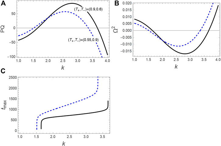
FIGURE 1. The regions of (un)stable electrostatic ion-acoustic modulated structures according to (A) the sign of the product $PQ$ and (B) the sign of both ${\text{Ω}}^2$ are plotted against the wavenumber k for different values of $\left(T_{+},T_{-}\right)$. Also, (C) the maximum value of modulational instability period $t_{\text{max}}$ is plotted against the wavenumber k for different values of $\left(T_{+},T_{-}\right)$. Note that the DRWs and DBs only exist in the regions that meet the instability conditions $\left(PQ>0\&{\text{ Ω}}^2<0\&t<t_{\text{max}}\right)$.

In the following sections, we devote our effort to solving Eq. 3 using two approximate methods to investigate the characteristic behavior of some modulated structures that propagate within such a model of DRWs and DBs (DABs and DKMBs), etc.

3 Rogue Waves and Breathers Solutions of Linear Damped NLSE

The two approximate methods used to find some approximate solutions for Eq. 3 are:

The first method is the semi-analytical method where the exact solution to the standard NLSE ($R=0$) is used to construct an approximate analytical solution to Eq. 3 without any iterations or use of computer code. In addition, the speed obtaining the result does not depend on the efficiency of the device.

The second method is a hybrid method between two numerical methods; the moving boundary method (MBM) and the finite difference method (FDM). Furthermore, in these methods, the exact solution to the standard NLSE ($R=0$) is used as the initial solution to finding the approximate numerical solutions to Eq. 3. In this case, the numerical solutions depend on a computer code and the accuracy depends on the number of iterations. The speed of running a code also depends on the efficiency of the device.

3.1 Analytical RWs and Breathers Solutions to the NLSE

It is obvious that the dissipation effect can be neglected ($R=0$) as compared to the dispersion effect, if the dispersion effect becomes more dominant than the dissipation effect. In this case, the linear damped NLSE (3) can be reduced to the following standard NLSE

where $\mho \in [L_i,L_f]\times [T_i,T_f]$ represents the physical domain of x and $t,$$L_i+L_f$ gives the length of the plasma system, and $T_f<t_{\text{max}}$, and for simplicity ${\text{Φ}}_{\delta }\equiv {\text{Φ}}_{\delta }\left(x,t\right)\equiv \text{Ψ}{|}_{R=0}$ is used.

The exact breathers and RWs solutions of Eq. 4 is Refs. 20 and 38.

where the growth factor $l_1=\sqrt{8\delta \left(1-2\delta \right)}$ and the instability wavenumber of the breathers is $l_2=\sqrt{4\left(1-2\delta \right)},$ and δ is a real and positive parameter ($\delta >0$) responsible for determining the type of breathers structures as follows: for $\delta >1/2,$ the time-periodic KMBs solution is covered as shown in Figure 2, for $0<\delta <1/2,$ the space-periodic ABs solution is obtained (see Figure 3), and the RW solution is covered for $\delta \to 1/2$ as illustrated in Figure 4. At $(x,t=0)$ and $\left(x=0,t=0\right)$, both the peaks ${\text{Φ}}_{\delta }\left(x,0\right)$ and the maximum amplitudes (the amplification) ${\text{Φ}}_{\delta -\text{Max}}$ of RWs and breathers (ABs and KMBs) are

and

It is also known that parameter δ is responsible for the periodicity of both KMBs and ABs, as depicted in Figure 3. An increase in δ leads to an increase in the number of periodicity for both KMBs (see Figure 5A) and ABs (see Figure 5B). Moreover, as seen from Figures 2–4 and Eq. 7 the maximum amplitude of RWs ${\text{Φ}}_{\delta \to \frac{1}{2}-\text{Max}}$ is larger than the ABs ${\text{Φ}}_{0<\delta <\frac{1}{2}-\text{Max}}$ but smaller than the KMBs ${\text{Φ}}_{\delta >\frac{1}{2}-\text{Max}}$ i.e., ${\text{Φ}}_{\delta >\frac{1}{2}-\text{Max}}>{\text{Φ}}_{\delta \to \frac{1}{2}-\text{Max}}>{\text{Φ}}_{0<\delta <\frac{1}{2}-\text{Max}}$.

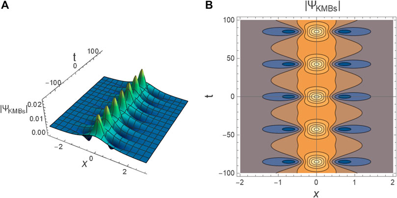
FIGURE 2. The profile of non-dissipative ($R=0$) KMBs $\left|{\text{Ψ}}_{DKMBs}\right|$ is plotted in the plane $\left(x,t\right)$ for $\left(T_{+},T_{-}\right)=\left(0.9,0.6\right)$ i.e., $\left(P,Q,k,\delta \right)$$=\left(-0.0522716,-1404.1,\mathrm{2,1}\right)$.

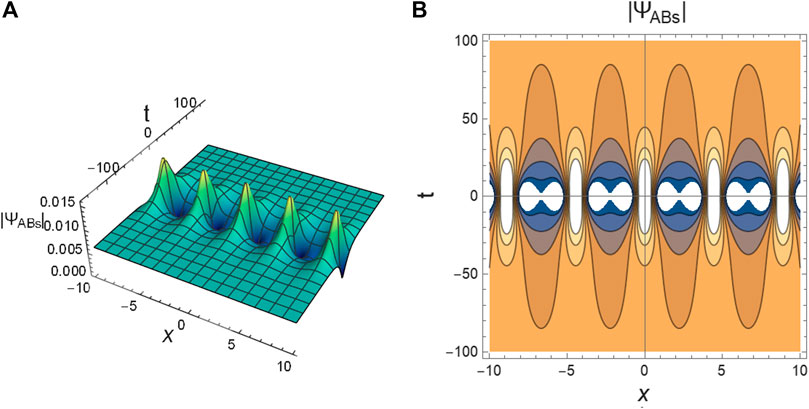
FIGURE 3. The profile of non-dissipative ($R=0$) ABs $\left|{\text{Ψ}}_{DABs}\right|$ is plotted in the plane $\left(x,t\right)$ for $\left(T_{+},T_{-}\right)=\left(0.9,0.6\right)$ i.e., $\left(P,Q,k,\delta \right)$$=\left(-0.0522716,-1404.1,\mathrm{2,0.25}\right)$.

FIGURE 4. The profile of non-dissipative ($R=0$) RWs $\left|{\text{Ψ}}_{DRWs}\right|$ is plotted in the plane $\left(x,t\right)$ for $\left(T_{+},T_{-}\right)=\left(0.9,0.6\right)$ i.e., $\left(P,Q,k,\delta \right)$$=(-0.0522716,-1404.1,2,\to 0.5)$.

FIGURE 5. The non-dissipative ($R=0$) KMBs and ABs solutions are plotted against $\left(x,t,\delta \right)$ for $\left(T_{+},T_{-}\right)=\left(0.9,0.6\right)$ i.e., $\left(P,Q,k\right)$$=\left(-0.0522716,-1404.1,2\right)$.

3.2 Semi-Analytical Solution of Dissipative RWs and Breathers

It is known that Eq. 3 is a non-integrable equation i.e., it has no analytical solution in its current form without using any transformation. So, in this section, we devote our efforts to obtain an approximate analytical solution for this equation. To do that let us suppose that $Q=0$, then Eq. 3 becomes

Also, suppose that $\varphi \equiv \varphi \left(x,t\right)$ is an exact analytical solution to

According to Eqs. 8, 9, the definition of $\text{Ψ}$ reads

where $f\equiv f\left(t\right)$ is a time-dependent function which will be determined later.

Inserting Eq. 10 into Eq. 8, we get

here, the prime “′” represents the derivative with respect to $t.$

It is clear that for $f^{\prime }+Rf=0$, we have

Then $\text{Ψ}=f\left(t\right)\varphi \left(x,t\right)$ becomes a solution to Eq. 8. This motivates us to seek an approximate analytical solution to Eq. 3 in the ansatz form

where $\text{Φ}\equiv \text{Φ}\left(x,t\right)$ represents any exact analytical solution to Eq. 4.

Inserting ansatz Eq. 13 into Eq. 3 and taking the following definition into account

we obtain

by integrating Eq. 16 once over t, yields

Finally, the semi-analytical solution to Eq. 3 for DRWs $\left(\delta \to 1/2\right),$ DKMBs $\left(\delta >1/2\right),$ and DABs $\left(0<\delta <1/2\right)$ can be expressed by

where ${\text{Φ}}_{\delta }$ is given by Eq. 5.

The residual associated to Eq. 3 reads

In view of Eq. 15, we get

From Eq. 20, we obtain

For example, the expression of the square residual error for the DRWs $\left(\delta =1/2\right)$ can be estimated from Eqs. 5, 21 as follows

By simplifying the square root of Eq. 22, we get

Similarly, the expression of the residual error for $\delta \ne 1/2$ can be estimated after some algebraic manipulations using Eqs. 5, 21 but the details are not inserted here because they are too large.

Let us introduce some numerical examples (or sometimes it is called experimental examples) to investigate the characteristic behavior of DRWs and DBs (DABs and DKMBs) to be able to evaluate the residual errors of solution Eq. 18. In the unstable region for the damped wave ($PQ>0$ & ${\text{Ω}}^2<0$ & $t<t_{\text{max}}$), the values of the physical plasma parameters $\left(T_{+},T_{-},k\right)=\left(0.9,0.6,2\right)$ give $\left(P,Q\right)\approx \left(-0.0522716,-1404.1\right)$. Also, for the same values of the last plasma parameters $\left(T_{+},T_{-}\right)=\left(0.9,0.6\right)$ and different values of wavenumber k, the values of both $R$ and $t_{\text{max}}$ could be obtained as given in the table below.$\left|{\text{Ψ}}_{DKMBs}\right|$, DABs $\left|{\text{Ψ}}_{DABs}\right|$, and DRWs $\left|{\text{Ψ}}_{DRWs}\right|$ are, respectively, illustrated in Figures 6–8 corresponding to the semi-analytical solution Eq. 18. Also, the impact of normalized ion-neutral collision frequencies ${\nu }_{\pm }$ on the profile of DKMBs $\left|{\text{Ψ}}_{DKMBs}\right|$ (similarly DABs $\left|{\text{Ψ}}_{DABs}\right|$ and DRWs $\left|{\text{Ψ}}_{DRWs}\right|$ but we have not included their illustrations here) is investigated as elucidated in Figure 9, for different values of ${\nu }_{\pm }$. It is observed that the KMBs create low intensity pulses with increasing R which has been confirmed in some laboratory experiments [41–44]. Moreover, for $\left(T_{+},T_{-},k\right)=\left(0.9,0.6,1.8\right)$ which means $\left(P,Q\right)\approx \left(-0.0608182,-525.935\right)$ and for different values of R, both the maximum local (at final time $T_f$) and maximum global (on the whole domain space-time domain $x_i\left(-10\right)\le x\le x_f$$\left(10\right)$ & $0\le \left|t\right|\le T_f\left(10\right)$) residual errors $\left(L_R\right)$ of the approximate analytical solution Eq. 18 are evaluated as shown in Figures 10, 11, respectively. These errors are estimated according to formula Eq. 21 for the solution Eq. 18. Furthermore, the functions of the maximum local and maximum global errors of solution Eq. 18 could be evaluated using the polynomials based on the Chebyshev approximation technique [18, 19]. The comparison between the maximum residual (local and global) errors $\left(L_R\right)$ using relation Eq. 22 and the errors functions evaluated by the Chebyshev approximation technique is illustrated in Figure 10 for the maximum local error and in Figure 11 for the maximum global error. It is observed that the results produced by relation Eq. 22 are in good agreement with the results obtained by Chebyshev polynomials. This enhances the high accuracy of the obtained semi-analytical solution Eq. 18. It should be noted here that the solution Eq. 18 could be used to explain and interpret the dissipative RWs and breathers that can occur and propagate in many branches of science such as optical fibers. Thus, any values for the coefficients P, Q, and R could be used for any application and not only in plasma physics which in our solution is considered to be stable with any values for P, Q, and R.

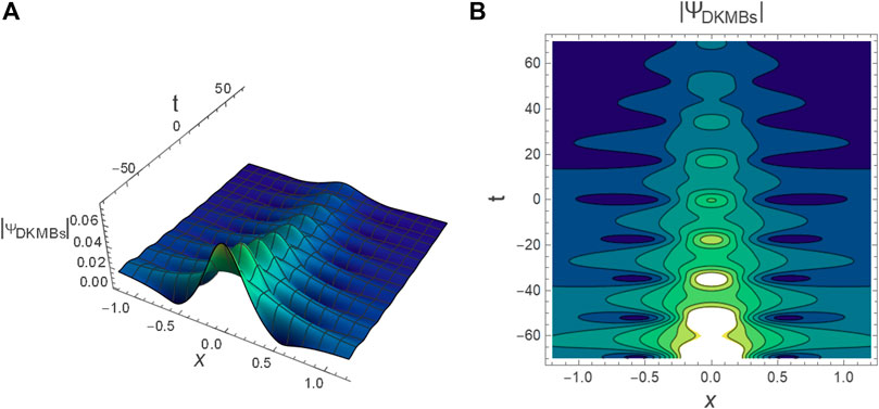
FIGURE 6. The profile of DKMBs $\left|{\text{Ψ}}_{DKMBs}\right|$ is plotted in the plane $\left(x,t\right)$ for $\left(P,Q,k,\delta ,R\right)$$=\left(-0.0522716,-1404.1,\mathrm{2,2,0.0136}\right)$. (A) Plot3D for DKMBs $\left|{\text{Ψ}}_{DKMBs}\right|$ and (B) Contourplot for DKMBs $\left|{\text{Ψ}}_{DKMBs}\right|$.

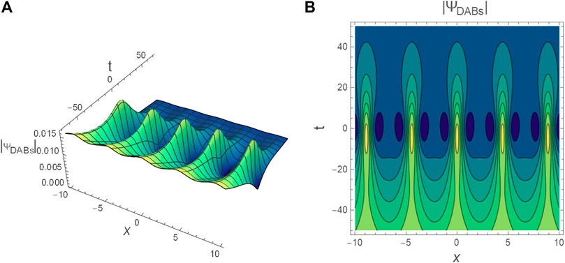
FIGURE 7. The profile of DABs $\left|{\text{Ψ}}_{DABs}\right|$ is plotted in the plane $\left(x,t\right)$ for $\left(P,Q,k,\delta ,R\right)$$=\left(-0.0522716,-1404.1,\mathrm{2,0.25},0.0136\right)$. (A) Plot3D for DABs $\left|{\text{Ψ}}_{DABs}\right|$ and (B) Contourplot for DABs $\left|{\text{Ψ}}_{DABs}\right|$.

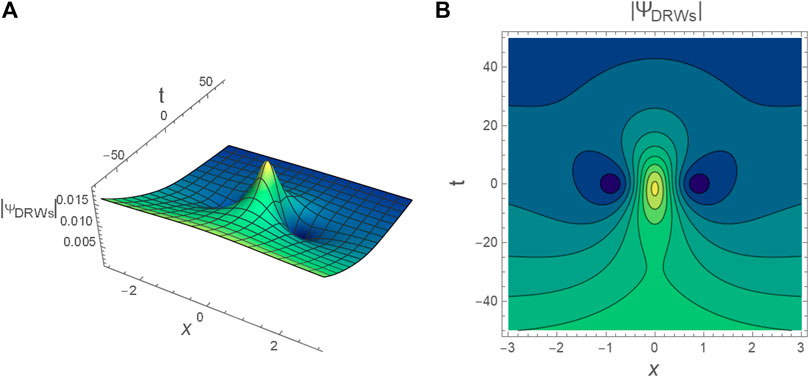
FIGURE 8. The profile of DRWs $\left|{\text{Ψ}}_{DRWs}\right|$ is plotted in the plane $\left(x,t\right)$ for $\left(P,Q,k,\delta ,R\right)$$=(-0.0522716,-1404.1,2,\to 0.5,0.0136)$. (A) Plot3D for DRWs $\left|{\text{Ψ}}_{DRWs}\right|$ and (B) Contourplot for DRWs $\left|{\text{Ψ}}_{DRWs}\right|$.

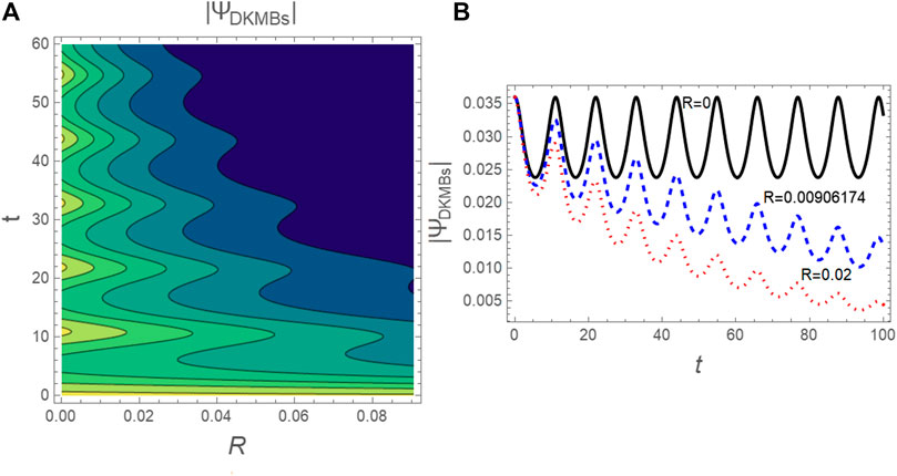
FIGURE 9. (A) The contourplot of DKMBs profile $\left|{\text{Ψ}}_{DKMBs}\right|$ according to the semi-analytical solution Eq. 18 is plotted in the plane $\left(t,R\right)$ and (B) The DKMBs profile $\left|{\text{Ψ}}_{DKMBs}\right|$ according to the semi-analytical solution Eq. 18 is plotted against t for different values of R. Here, $\left(P,Q,k,\delta \right)$$=\left(-0.0522716,-1404.1,\mathrm{2,3}\right)$.

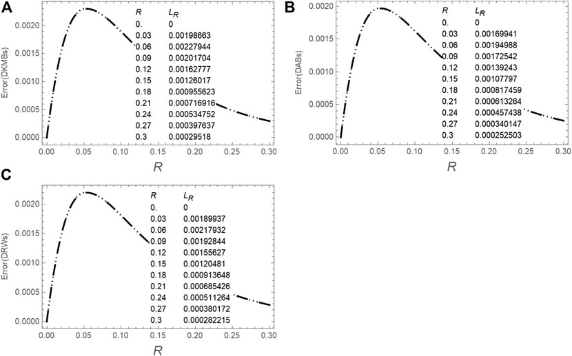
FIGURE 10. A comparison between the maximum local error (at final time $T_f=10$) of the semi-analytical solution Eq. 18 according to the relation Eq. 22 and the function of the local error related to the final time $T_f=10$ based on Chebyshev approximation technique is plotted against R for (A) DKMBs $\delta =0.75$, (B) DABs $\delta =0.25$, and (C) DRWs $\delta \to 0.5$. Here, $\left(T_{+},T_{-}\right)=\left(0.9,0.6\right)$ i.e., $\left(P,Q,k\right)$$=\left(-0.0608182,-525.935,1.8\right)$.

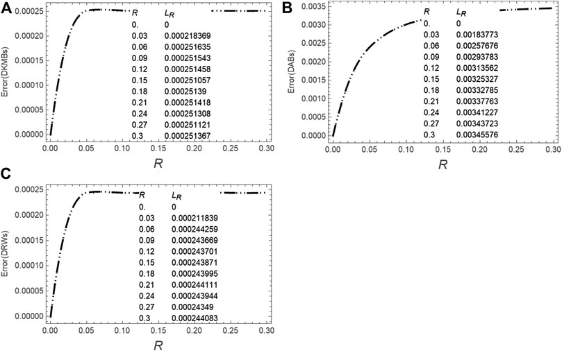
FIGURE 11. A comparison between the maximum global error (on the whole domain space-time domain $-10\le x\le 10$ & $0\le \left|t\right|\le 10$) of the semi-analytical solution Eq. 18 according to the relation Eq. 22 and the function of the global error related to the whole domain space-time domain based on Chebyshev approximation technique is plotted against R for (A) DKMBs $\delta =0.75$, (B) DABs $\delta =0.25$, and (C) DRWs $\delta \to 0.5$. Here, $\left(T_{+},T_{-}\right)=\left(0.9,0.6\right)$ i.e., $\left(P,Q,k\right)$$=\left(-0.0608182,-525.935,1.8\right)$.

4 Numerical Approximate Solutions

Let us define the following initial value problem (i.v.p.)

which is subjected to the initial condition

and the Dirichlet boundary conditions

where $0<\left|t\right|<t_{\text{max}}$, $\mho =[L_i,L_f]\times [T_i,T_f]$ represents the space-time domain, $L_i+L_f$ denotes the plasma system length, and $\text{Φ}\left(x\right)$ indicates any exact analytical solution to the undamped NLSE i.e., Eq. 24 for $R=0$. As a special case, the RW and breathers solutions given in Eq. 5 could be used as the initial solution for Eq. 24 at a certain time (say $t=T_i$).

4.1 Finite Differences Method

To solve the i. v.p. Eqs. 24–26 numerically using the FDM. [40, 56], we first divide the complex function $\text{Ψ}\equiv \text{Ψ}\left(x,t\right)$ into real and imaginary parts

where $U\equiv U\left(x,t\right)=\text{Re}\left(\text{Φ}\right)$ and $V\equiv V\left(x,t\right)=\text{Im}\left(\text{Φ}\right)$. As a special case, the values of U and V could be obtained from solution Eq. 5 as

and

By substituting Eq. 27 into Eq. 24 and separating the obtained equation into real and imaginary parts, we get

To apply the FDM, the following discretization for the space-time domain $\text{Ω}$ are introduced

where m and n indicate the number of iterations. According to the FDM, the values of the space and time derivatives can be found in detail in Ref. 57.

It should be mentioned here that the FDM gives good results for small time intervals, and this is consistent with the values of observed time for the existing acoustic-waves in the plasma model. In general, the large time intervals give ill conditioned systems of nonlinear equations and they are associated to stiffness, causing numerical instability. On the other hand, for large time intervals, the hybrid MBM-FDM works significantly better than FDM.

4.2 The Mechanism of the Moving Boundary Method to Analyze the Linear Damped NLSE

To improve the approximate numerical solution that has been obtained by the FDM, the MBM is introduced to achieve this purpose. In this method we divide the whole-time interval $T_i\le t\le T_f$ into subintervals of length $d\tau =\left(T_f-T_i\right)/n$; say $T_i=t_0<t_1<t_2<\cdots <t_j<\cdots <t_n=T_f$, where $t_j=T_i+jd\tau$ ($j=\mathrm{0,1},\dots ,n$). Thereafter, we try to find the solution through the subintervals say: ${\text{Ψ}}_0\left(x,T_i\right)={\text{Φ}}_0\left(x,T_i\right)$ in the subinterval $\left[T_i,t_1\right]\times \left[L_i,L_f\right]$, ${\text{Ψ}}_1\left(x,t_1\right)={\text{Φ}}_1\left(x\right)$ in the next subinterval $\left[t_1,t_2\right]\times \left[L_i,L_f\right]$, $\cdots$ until arrive to the final solution ${\text{Ψ}}_j\left(x,t_j\right)={\text{Φ}}_j\left(x\right)$ in the final subinterval $\left[t_j,t_{j+1}\right]\times \left[L_i,L_f\right]$ with $T_f=T_i+nd\tau \equiv t_n$ where $j=\mathrm{0,1,2,3},n-1$. Thus, the solution on the whole domain $\text{Π}=\left[X_i,X_f\right]\times \left[T_i,T_f\right]$ could be written in the form of a linear combination of characteristic functions such as

with

To illustrate the high accuracy and effectiveness of the hybrid MBM-FDM, we present some numerical examples. For instance, let us analyze the i. v.p. Eqs. 24–26 using the hybrid MBM-FDM and make a comparison between the semi-analytical solution Eq. 18 and the numerical approximate solution Eq. 32 for modeling the DRWs and DBs. The profiles of the DRWs, DABs, and DKMBs are plotted in Figures 12–14, respectively, according to the semi-analytical solution Eq. 18 and approximate numerical solution Eq. 32 for any random values to the coefficients $\left(P,Q,R\right)$ that meet the MI criteria $\left(PQ>0\&{\text{ Ω}}^2<0\&t<t_{\text{max}}\right)$. It is observed that both the amplitude and the width of DRWs, DABs, and DKMBs decrease gradually with the increase of the collisional frequency. Generally, the waves decay with an increasing damping coefficient R. Physically, increasing R leads to dissipating wave energy, and consequently it leads to a decrease in the nonlinearity, which leads to the decay of these waves. The local errors (at a certain value of time (say $T_f$)) of both semi-analytical and numerical solutions are also estimated according to Eq. 19 as shown in Table 1.

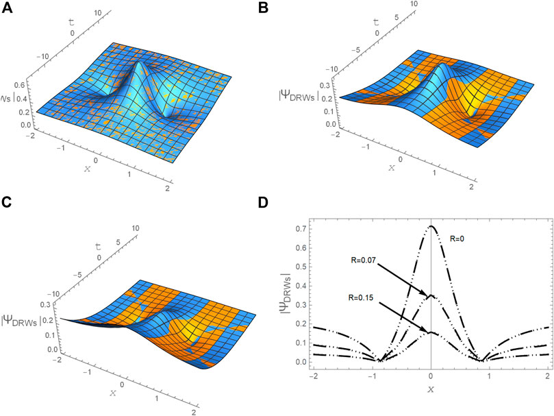
FIGURE 12. A comparison between the semi-analytical solution Eq. 18 and the approximate numerical solution Eq. 32 for DRWs is plotted in the plane $\left(x,t\right)$ for (A)$R=0$, (B)$R=0.07$, and (C)$R=0.15$. In Figure 12D the comparison between the two approximate solutions (dashed curve for solution Eq. 18 and dotted curve for solution Eq. 32) is plotted against x for different values of R. Here, $\left(P,Q\right)\approx \left(-0.148,-2.6\right)$.

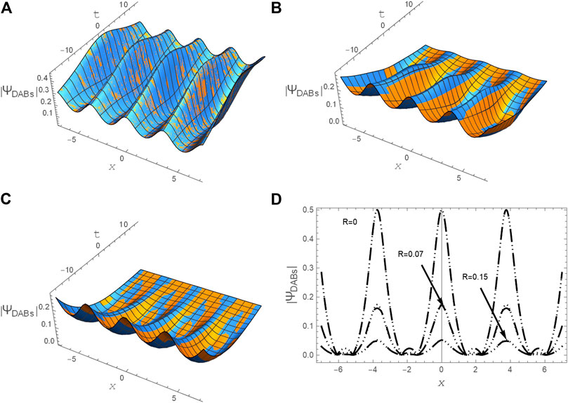
FIGURE 13. A comparison between the semi-analytical solution Eq. 18 and the numerical approximate solution Eq. 32 for DABs ($\delta =0.15$) is plotted in the plane $\left(x,t\right)$ for (A)$R=0$, (B)$R=0.07$, and (C)$R=0.15$. In Figure 13D the comparison between the two approximate solutions (dashed curve for solution Eq. 18 and dotted curve for solution Eq. 32) is plotted against x for different values of R. Here, $\left(P,Q\right)\approx \left(-0.148,-2.6\right)$.

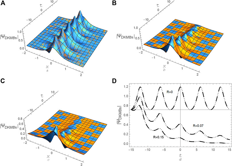
FIGURE 14. A comparison between the semi-analytical solution Eq. 18 and the numerical approximate solution Eq. 32 (Dotted curve) for DKMBs ($\delta =2$) is plotted in the plane $\left(x,t\right)$ for (A)$R=0$, (B)$R=0.07$, and (C)$R=0.15$. In Figure 14D the comparison between the two approximate solutions (dashed curve for solution Eq. 18 and dotted curve for solution Eq. 32) is plotted against x for different values of R. Here, $\left(P,Q\right)\approx \left(-0.148,-2.6\right)$.

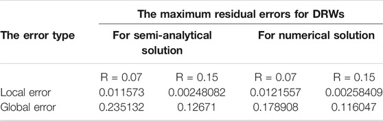
TABLE 1. The maximum local and global residual errors of both approximate analytical and numerical solutions for DRWs have been estimated for $\left(P,Q\right)\approx \left(-0.148,-2.6\right)$ and with different values to R.

The numerical values of the maximum local and global errors of both approximate analytical and numerical solutions for DRWs ($\delta \to 1/2$) are presented in Table 1. It is noted that both approximate analytical and numerical solutions give excellent results as illustrated in Table 1. In general, our numerical method does not require a highly efficient device whereas the calculations of this method could be performed by simply using a personal computer. Moreover, the semi-analytical solution provides excellent results, and it is more stable.

5 Summary

The propagation of electrostatic nonlinear dissipative envelope structures including dissipative rogue waves (DRWs) and dissipative breathers (DBs) in nonlinear and dispersive mediums, such as unmagnetized collisional pair-ion plasmas composed of warm positive and negative ions, has been investigated analytically and numerally. Sikdar et al. [49] reduced the fluid governing equations of this model to the linear damped nonlinear Schrödinger equation (NLSE) using a reductive perturbation technique (the derivative expansion method) to study both collisionless and collisional envelope solitons (bright and dark solitons). In our study, we used the linear damped NLSE to study both DRWs and DBs in any nonlinear and dispersive medium. The exact analytical solution of the linear damped NLSE has not been possible until now, due to the presence of the damping term. Consequently, two effective methods were devoted to model and solve this problem. The first one is called the semi-analytical method which was built depending on the exact analytical solution of the standard NLSE (without linear damping term). The semi-analytical solution of the linear damped NLSE is considered to be the first attempt at modeling the DRWs and DBs in plasmas or in any other physical medium like optical fiber and so on. In the second method, the numerical simulation solution to the linear damped NLSE using the hybrid new method namely, the moving boundary method (MBM) with the finite difference method (FDM), has been carried out. In this method, the exact solution of the standard NLSE is used as the initial condition to solve the linear damped NLSE using the hybrid MBM-FDM. Moreover, both the local (at final time) and global (on the whole domain space-time domain) maximum residual errors of the approximate solutions have been estimated precisely depending on the physical parameters of the model under consideration. Furthermore, the functions of both the local and global residual errors for solution Eq. 18 have been evaluated using the polynomials based on the Chebyshev approximation technique. The comparison between the error of both the semi-analytical and numerical solutions have also been examined and it was found that the error is very small, which enhances the high accuracy of the two solutions. This investigation helped us to understand the dynamic mechanism of modulated envelope structures in a strongly coupled complex plasma and many other branches of science such as optical fiber or mechanical fluid, etc.

Data Availability Statement

The original contributions presented in the study are included in the article/Supplementary Material, further inquiries can be directed to the corresponding author.

Author Contributions

All authors listed have made a substantial, direct, and intellectual contribution to the work and approved it for publication.

Funding

Taif University Researchers Supporting Project number (TURSP-2020/275), Taif University, Taif, Saudi Arabia.

Conflict of Interest

The authors declare that the research was conducted in the absence of any commercial or financial relationships that could be construed as a potential conflict of interest.

References

1. Wazwaz AM. Partial differential equations and solitary waves theory. Beijing, USA: Higher Education Press (2009).
2. Wazwaz A-M. A variety of optical solitons for nonlinear Schrödinger equation with detuning term by the variational iteration method. Optik (2019) 196:163–9. doi:10.1016/j.ijleo.2019.163169
3. Dai C-Q, Fan Y, Zhang N. Re-observation on localized waves constructed by variable separation solutions of (1+1)-dimensional coupled integrable dispersionless equations via the projective Riccati equation method. Appl Math Lett (2019) 96:20–6. doi:10.1016/j.aml.2019.04.009
4. Chen Y-X, Xu F-Q, Hu Y-L. Excitation control for three-dimensional Peregrine solution and combined breather of a partially nonlocal variable-coefficient nonlinear Schrödinger equation. Nonlinear Dynam (2019) 95:1957. doi:10.1007/s11071-018-4670-7
5. Dai C-Q, Fan Y, Wang Y-Y. Three-dimensional optical solitons formed by the balance between different-order nonlinearities and high-order dispersion/diffraction in parity-time symmetric potentials. Nonlinear Dynam (2019) 98:489–99. doi:10.1007/s11071-019-05206-z
6. Dai C-Q, Liu J, Fan Y, Yu D-G. Two-dimensional localized Peregrine solution and breather excited in a variable-coefficient nonlinear Schrödinger equation with partial nonlocality. Nonlinear Dynam (2017) 88:1373–83. doi:10.1007/s11071-016-3316-x
7. Dai C-Q, Wang Y-Y, Fan Y, Yu D-G. Reconstruction of stability for Gaussian spatial solitons in quintic-septimal nonlinear materials under $${{\varvec{\mathcal {P}}}}{\varvec{\mathcal {T}}}$$ P T -symmetric potentials. Nonlinear Dynam (2018) 92:1351–8. doi:10.1007/s11071-018-4130-4
8. Dai C-Q, Zhang J-F. Controlling effect of vector and scalar crossed double-Ma breathers in a partially nonlocal nonlinear medium with a linear potential. Nonlinear Dynam (2020) 100:1621–8. doi:10.1007/s11071-020-05603-9
9. Yu L-J, Wu G-Z, Wang Y-Y, Chen Y-X. Traveling wave solutions constructed by Mittag-Leffler function of a (2 + 1)-dimensional space-time fractional NLS equation. Results Phys (2020) 17:103156. doi:10.1016/j.rinp.2020.103156
10. Wu G-Z, Dai C-Q. Nonautonomous soliton solutions of variable-coefficient fractional nonlinear Schrödinger equation. Appl Math Lett (2020) 106:106365. doi:10.1016/j.aml.2020.106365
11. Ruderman MS, Talipova T, Pelinovsky E. Dynamics of modulationally unstable ion-acoustic wavepackets in plasmas with negative ions. J Plasma Phys (2008) 74:639–56. doi:10.1017/s0022377808007150
12. Ruderman MS. Freak waves in laboratory and space plasmas. Eur Phys J Spec Top (2010) 185:57–66. doi:10.1140/epjst/e2010-01238-7
13. Lü X, Tian B, Xu T, Cai K-J, Liu W-J. Analytical study of the nonlinear Schrödinger equation with an arbitrary linear time-dependent potential in quasi-one-dimensional Bose-Einstein condensates. Ann Phys (2008) 323:2554–65. doi:10.1016/j.aop.2008.04.008
14. Onorato M, Residori S, Bortolozzo U, Montina A, Arecchi FT. Rogue waves and their generating mechanisms in different physical contexts. Phys Rep (2013) 528:47–89. doi:10.1016/j.physrep.2013.03.001
15. Chabchoub A, Hoffmann N, Onorato M, Slunyaev A, Sergeeva A, Pelinovsky E, et al. Observation of a hierarchy of up to fifth-order rogue waves in a water tank. Phys Rev E – Stat Nonlinear Soft Matter Phys (2012) 86, 056601. doi:10.1103/PhysRevE.86.056601
16. Xu G, Chabchoub A, Pelinovsky DE, Kibler B. Observation of modulation instability and rogue breathers on stationary periodic waves. Phys Rev Res (2020) 2:033528. doi:10.1103/physrevresearch.2.033528
17. Biswas A. Chirp-free bright optical soliton perturbation with Chen-Lee-Liu equation by traveling wave hypothesis and semi-inverse variational principle. Optik (2018) 172:772–6. doi:10.1016/j.ijleo.2018.07.110
18. Fox L, Parker IB (1968). Chebyshev polynomials in numerical analysis. London: Oxford University Press.
19. Clement PR. The Chebyshev approximation method. Q Appl Math (1953) 11:167. doi:10.1090/qam/58024
20. Kibler B, Fatome J, Finot C, Millot G, Genty G, Wetzel B, et al. Observation of Kuznetsov-Ma soliton dynamics in optical fibre. Sci Rep (2012) 2:463. doi:10.1038/srep00463
22. Chabchoub A, Hoffmann NP, Akhmediev N. Rogue wave observation in a water wave tank. Phys Rev Lett (2011) 106(20):204502. doi:10.1103/PhysRevLett.106.204502
23. Yan Z. Vector financial rogue waves. Phys Lett (2011) 375:4274–9. doi:10.1016/j.physleta.2011.09.026
24. Kibler B, Fatome J, Finot C, Millot G, Dias F, Genty G, et al. The Peregrine soliton in nonlinear fibre optics. Nat Phys (2010) 6:790–5. doi:10.1038/nphys1740
25. Lecaplain C, Grelu P, Soto-Crespo JM, Akhmediev N. Dissipative rogue waves generated by chaotic pulse bunching in a mode-locked laser. Phys Rev Lett (2012) 108:233901. doi:10.1103/PhysRevLett.108.233901
26. Solli DR, Ropers C, Koonath P, Jalali B. Optical rogue waves. Nature (2018) 450:1054–7. doi:10.1038/nature06402
28. Stenflo L, Marklund M. Rogue waves in the atmosphere. J Plasma Phys (2010) 76:293–5. doi:10.1017/s0022377809990481
29. Bailung H, Sharma SK, Nakamura Y. Observation of peregrine solitons in a multicomponent plasma with negative ions. Phys Rev Lett (2011) 107:255005. doi:10.1103/PhysRevLett.107.255005
30. Sharma SK, Bailung H. Observation of hole Peregrine soliton in a multicomponent plasma with critical density of negative ions. J Geophys Res Space Phys (2013) 118(2):919–24. doi:10.1002/jgra.50111
31. Pathak P, Sharma SK, Nakamura Y, Bailung H. Observation of second order ion acoustic Peregrine breather in multicomponent plasma with negative ions. Phys Plasmas (2016) 23:022107. doi:10.1063/1.4941968
32. Pathak P, Sharma SK, Nakamura Y, Bailung H. Observation of ion acoustic multi-Peregrine solitons in multicomponent plasma with negative ions. Phys Lett (2017) 381:4011–18. doi:10.1016/j.physleta.2017.10.046
33. Akhmediev N, Soto-Crespo JM, Ankiewicz A. Extreme waves that appear from nowhere: on the nature of rogue waves. Phys Lett (2009) 373.(25):2137–45. doi:10.1016/j.physleta.2009.04.023
34. Demircan A, Amiranashvili S, Brée C, Mahnke C, Mitschke F, Steinmeyer G. Rogue events in the group velocity horizon. Sci Rep (2012) 2:850. doi:10.1038/srep00850
35. Dysthe KB, Trulsen K. Note on breather type solutions of the NLS as models for freak-waves. Phys Scripta (1999) T82:48. doi:10.1238/physica.topical.082a00048
36. Li M, Shui J-J, Xu T. Generation mechanism of rogue waves for the discrete nonlinear Schrödinger equation. Appl Math Lett (2018) 83:110–5. doi:10.1016/j.aml.2018.03.018
37. Li M, Shui J-J, Huang Y-H, Wang L, Li H-J. Localized-wave interactions for the discrete nonlinear Schrödinger equation under the nonvanishing background. Phys Scripta (2018) 93(11):115203. doi:10.1088/1402-4896/aae213
38. Akhmediev N, Ankiewicz A, Soto-Crespo JM. Rogue waves and rational solutions of the nonlinear Schrödinger equation. Phys Rev E – Stat Nonlinear Soft Matter Phys (2009) 80, 026601. doi:10.1103/PhysRevE.80.026601
39. Guob S, Mei L. Three-dimensional dust-ion-acoustic rogue waves in a magnetized dusty pair-ion plasma with nonthermal nonextensive electrons and opposite polarity dust grains. Phys Plasmas (2014) 21:082303. doi:10.1063/1.4891879
40. Delfour M, Fortin M, Payr G. Finite-difference solutions of a non-linear Schrödinger equation. J Comput Phys (1981) 44:277–88. doi:10.1016/0021-9991(81)90052-8
41. Lecaplain C, Grelu P, Soto-Crespo JM, Akhmediev N. Dissipative rogue waves generated by chaotic pulse bunching in a mode-locked laser. Phys Rev Lett (2012) 108:233901. doi:10.1103/PhysRevLett.108.233901
42. Lecaplain C, Grelu Ph, Soto-Crespo JM, Akhmediev N. Dissipative rogue wave generation in multiple-pulsing mode-locked fiber laser. J Optic (2013) 15:064005. doi:10.1088/2040-8978/15/6/064005
43. Liu M, Cai ZR, Hu S, Luo AP, Zhao CJ, Zhang H, et al. Dissipative rogue waves induced by long-range chaotic multi-pulse interactions in a fiber laser with a topological insulator-deposited microfiber photonic device. Opt Lett (2015) 40:4767–70. doi:10.1364/OL.40.004767
44. Liu M, Luo AP, Xu WC, Luo ZC. Dissipative rogue waves induced by soliton explosions in an ultrafast fiber laser. Opt Lett (2016) 41:3912–15. doi:10.1364/OL.41.003912
45. Onorato M, Proment D. Approximate rogue wave solutions of the forced and damped nonlinear Schrödinger equation for water waves. Phys Lett (2012) 376:3057. doi:10.1016/j.physleta.2012.05.063
46. Guo S, Mei L. Modulation instability and dissipative rogue waves in ion-beam plasma: roles of ionization, recombination, and electron attachment. Phys Plasmas (2014) 21:112303. doi:10.1063/1.4901037
47. Amin MR. Modulation of a compressional electromagnetic wave in a magnetized electron-positron quantum plasma. Phys Rev E – Stat Nonlinear Soft Matter Phys (2015) 92, 033106. doi:10.1103/PhysRevE.92.033106
48. El-Tantawy SA. Ion-acoustic waves in ultracold neutral plasmas: modulational instability and dissipative rogue waves. Phys Lett (2017) 381:787. doi:10.1016/j.physleta.2016.12.052
49. Sikdar A, Adak A, Ghosh S, Khan M. Electrostatic wave modulation in collisional pair-ion plasmas. Phys Plasmas (2018) 25:052303. doi:10.1063/1.4997224
50. El-Tantawy SA, Salas AH, Hammad Mm. A, Ismaeel SME, Moustafa DM, El-Awady EI. Impact of dust kinematic viscosity on the breathers and rogue waves in a complex plasma having kappa distributed particles. Waves Random Complex Media (2019) 1–21. doi:10.1080/17455030.2019.1698790
51. Adak A, Ghosh S, Chakrabarti N. Ion acoustic shock wave in collisional equal mass plasma. Phys Plasmas (2015) 22:102307. doi:10.1063/1.4933356
52. Sarkar S, Adak A, Ghosh S, Khan M. Ion acoustic wave modulation in a dusty plasma in presence of ion loss, collision and ionization. J Plasma Phys (2016) 82:905820504. doi:10.1017/s0022377816000799
53. Saini NS, Kourakis I. Dust-acoustic wave modulation in the presence of superthermal ions. Phys Plasmas (2008) 15:123701. doi:10.1063/1.3033748
54. Xue J-K. Modulation of dust acoustic waves with non-adiabatic dust charge fluctuations. Phys Lett (2003) 320:226–33. doi:10.1016/j.physleta.2003.11.018
55. Kui XJ. Modulational instability of dust ion acoustic waves in a collisional dusty plasma. Commun Theor Phys (2003) 40:717–20. doi:10.1088/0253-6102/40/6/717
56. Griffiths DF, Mitchell AR, Morris JL. A numerical study of the nonlinear Schrödinger equation. Comput Methods Appl Mech Eng (1984) 45:177–215. doi:10.1016/0045-7825(84)90156-7
Keywords: semi-analytical solution, finite difference method, dissipative rogue waves and breathers, moving boundary method, collisional pair-ion plasmas
Citation: El-Tantawy SA, Salas AH and Alharthi MR (2021) On the Analytical and Numerical Solutions of the Linear Damped NLSE for Modeling Dissipative Freak Waves and Breathers in Nonlinear and Dispersive Mediums: An Application to a Pair-Ion Plasma. Front. Phys. 9:580224. doi: 10.3389/fphy.2021.580224
Received: 05 July 2020; Accepted: 07 January 2021;
Published: 18 February 2021.
Edited by:
Bertrand Kibler, UMR6303 Laboratoire Interdisciplinaire Carnot de Bourgogne (ICB), FranceReviewed by:
Chao-QIng Dai, Zhejiang Agriculture and Forestry University, ChinaSamiran Ghosh, University of Calcutta, India
Copyright © 2021 El-Tantawy, Salas and Alharthi. This is an open-access article distributed under the terms of the Creative Commons Attribution License (CC BY). The use, distribution or reproduction in other forums is permitted, provided the original author(s) and the copyright owner(s) are credited and that the original publication in this journal is cited, in accordance with accepted academic practice. No use, distribution or reproduction is permitted which does not comply with these terms.
*Correspondence: S. A. El-Tantawy, samireltantawy@yahoo.com