the Creative Commons Attribution 4.0 License.
the Creative Commons Attribution 4.0 License.
 | 18 Feb 2021
Towards accurate and practical drone-based wind measurements with an ultrasonic anemometer
William Thielicke
Waldemar Hübert
Ulrich Müller
Michael Eggert
Paul Wilhelm
Wind data collection in the atmospheric boundary layer benefits from short-term wind speed measurements using unmanned aerial vehicles. Fixed-wing and rotary-wing devices with diverse anemometer technology have been used in the past to provide such data, but the accuracy still has the potential to be increased. A lightweight drone for carrying an industry-standard precision sonic anemometer was developed. Accuracy tests have been performed with the isolated anemometer at high tilt angles in a calibration wind tunnel, with the drone flying in a large wind tunnel and with the full system flying at different heights next to a bistatic lidar reference.
The propeller-induced flow deflects the air to some extent, but this effect is compensated effectively. The data fusion shows a substantial reduction of crosstalk (factor of 13) between ground speed and wind speed. When compared with the bistatic lidar in very turbulent conditions, with a 10 s averaging interval and with the unmanned aerial vehicle (UAV) constantly circling around the measurement volume of the lidar reference, wind speed measurements have a bias between −2.0 % and 4.2 % (root-mean-square error (RMSE) of 4.3 % to 15.5 %), vertical wind speed bias is between −0.05 and 0.07 m s−1 (RMSE of 0.15 to 0.4 m s−1), elevation bias is between −1 and 0.7∘ (RMSE of 1.2 to 6.3∘), and azimuth bias is between −2.6 and 7.2∘ (RMSE of 2.6 to 8.0∘). Key requirements for good accuracy under challenging and dynamic conditions are the use of a full-size sonic anemometer, a large distance between anemometer and propellers, and a suitable algorithm for reducing the effect of propeller-induced flow.
The system was finally flown in the wake of a wind turbine, successfully measuring the spatial velocity deficit and downwash distribution during forward flight, yielding results that are in very close agreement to lidar measurements and the theoretical distribution. We believe that the results presented in this paper can provide important information for designing flying systems for precise air speed measurements either for short duration at multiple locations (battery powered) or for long duration at a single location (power supplied via cable). UAVs that are able to accurately measure three-dimensional wind might be used as a cost-effective and flexible addition to measurement masts and lidar scans.


1.1 Wind speed measurements
Measurements of wind characteristics are important in the environmental science of the atmospheric boundary layer (ABL). They are crucial for predictions of meteorological processes (e.g. Lauer and Fengler, 2017), optimization of wind turbine performance (e.g. Wagner et al., 2009), understanding wake interactions with the ABL in large wind farms (Kumer et al., 2015; Lungo, 2016; Li et al., 2016) and as boundary conditions for simulations of gas dispersion in the ABL (e.g. Labovský and Jelemenský, 2011). Popular systems for getting the required wind velocity data in different regions of the ABL are traditional mast-mounted anemometers (mostly cup and sonic anemometers, e.g. Izumi and Barad, 1970), balloons (e.g. Scoggins, 1965), sonic detecting and ranging (SODAR; Reitebuch and Emeis, 1998) and light detection and ranging (lidar, e.g. Bilbro et al., 1984). The methods are suitable for measurements of different ranges of temporal and spatial scales, they result in complementary data and are often subject to comparisons (e.g. Barthelmie et al., 2014).
1.2 Unmanned aerial vehicles as sensor platforms
Despite the large variation of existing measurement techniques, there is still a gap in the wind data collection in the ABL, driving the development of small unmanned aerial vehicles (UAVs) that are equipped with sensors measuring wind velocities (Ivey et al., 2014; Elston et al., 2014; Lauer and Fengler, 2017; Prudden et al., 2018; Rautenberg et al., 2018; Barbieri et al., 2019). These UAVs are less suitable for long-term measurements as the endurance is typically limited. However, they have three-dimensional (3-D) mobility, are easy to deploy, inexpensive and flexible to operate, and provide time- and space-resolved measurements of wind speeds (e.g. Nichols et al., 2017). They are versatile and can easily be equipped with additional sensors to map further air properties in 3-D space. UAVs are therefore believed to contribute valuable data to research in the ABL (e.g. Van den Kroonenberg et al., 2008; Wildmann et al., 2014; Prudden et al., 2018; Rautenberg et al., 2018; Barbieri et al., 2019).
There are two fundamental types that are suitable for atmospheric wind measurements: fixed-wing and rotary-wing UAVs. In fixed-wing UAVs, the wings provide the force (L) to counter weight (W). Propellers supply thrust (T) that is needed to overcome the drag (D) of the aircraft; hence, thrust is proportional to . In contrast, rotary-wing UAVs provide all the force that is needed to offset weight by the thrust of propellers; hence, T is proportional to W. As the lift-to-drag ratio () of fixed-wing UAVs can easily exceed unity and often reaches values of about 10 (Thielicke, 2014), the thrust requirement of similar-sized fixed-wing UAVs is significantly smaller. Power is thrust multiplied by speed; hence, the power requirement of fixed-wing UAVs can be much lower than in rotary-wing UAVs at similar flight speeds (see Fig. 1). This makes fixed-wing UAVs very suitable for measuring tasks that require long flight times and large areas to be covered (Thielicke, 2014), especially in areas with high wind speeds that require elevated air speeds of the vehicle.
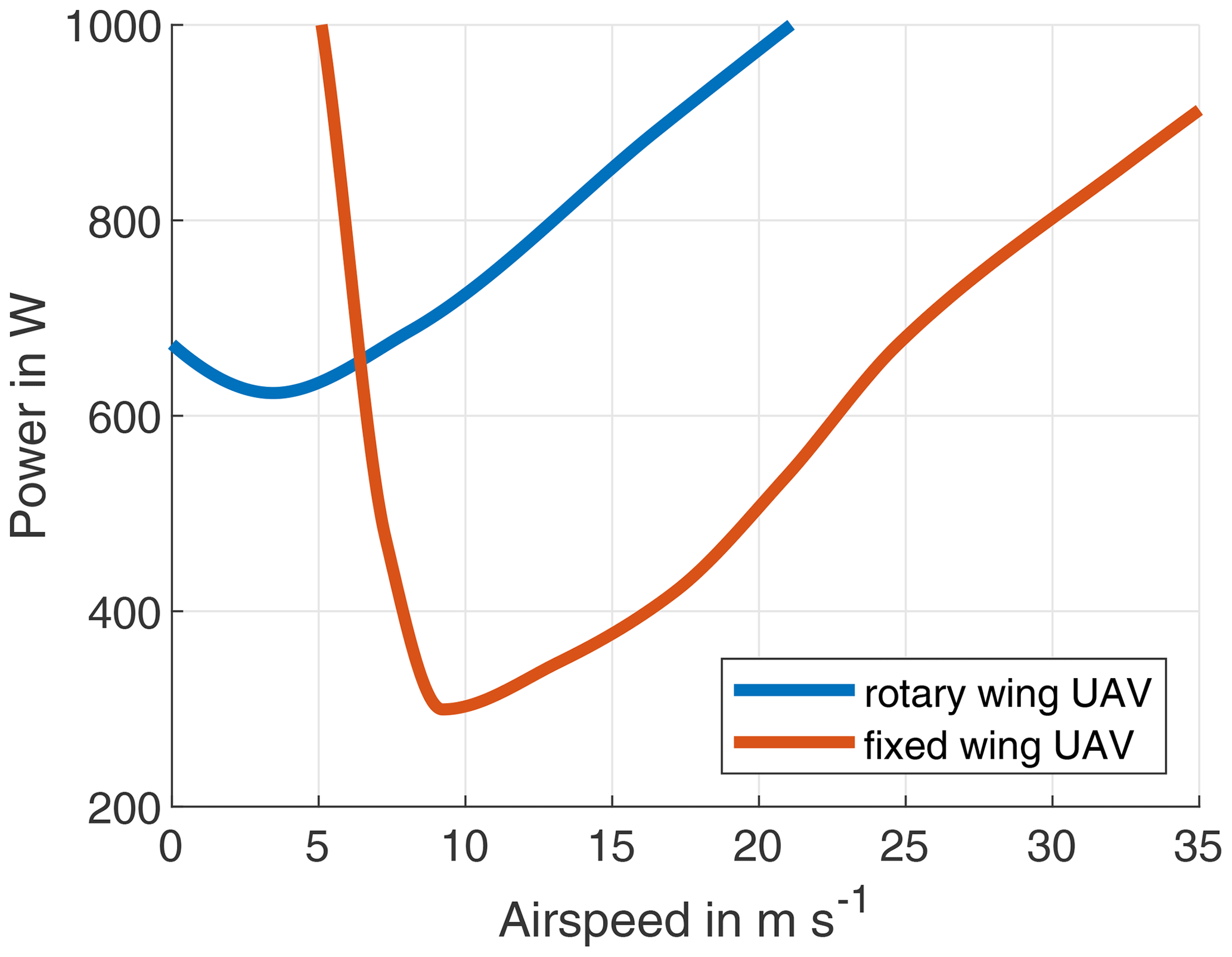
Figure 1Power requirement of fixed-wing vs. rotary-wing UAVs with the same weight (redrawn from Poh and Poh, 2014).
Rotary-wing UAVs have a lower endurance, typically by a factor of < 0.5. They are however easier to deploy and operate, have the capability to hover on the spot and are much more manoeuvrable (Thielicke, 2014). Therefore, they can measure wind speeds close to structures and perform measurements at a single spot for prolonged periods. These are desirable properties, e.g. when validating wind measurements of the UAV in proximity to traditional anemometers in the field.
1.3 UAV-based wind speed measurements
Wind can be determined using two different approaches in UAVs: indirect methods measure the response of the UAV to the wind and can determine wind speed, azimuth and elevation directly from the sensors that are also used to control the UAV (e.g. Neumann et al., 2010; Johansen et al., 2015; Xiang et al., 2016; Lauer and Fengler, 2017; Donnell et al., 2018). Such methods require knowledge about the inertia and drag coefficients of the UAV in a larger set of situations. These are not trivial to determine but have a large impact on the accuracy of wind measurements. Using this approach can increase the flight time and the maximum sustainable wind speed, as no additional sensor must be carried.
Direct methods use dedicated wind sensors that are mounted to the UAV. Suitable sensors should be lightweight, robust and measure a 3-D wind vector. Together with the 3-D ground speed vector of the UAV, wind speed and direction can be derived by simple vector addition. If the sensor is mounted on a gimbal, ensuring zero pitch and roll angle during flight, then a two-dimensional sensor can be sufficient to measure 2-D wind speed. In practice, the fusion of vehicle speed and wind speed can yield erroneous results due to errors in wind sensing and vehicle state estimation. These errors become visible as periodic signals in the wind data having a similar frequency as the vehicle speed, attitude or position (Nichols et al., 2017).
Several types of sensors have already been used to measure wind speeds with fixed-wing and rotary-wing UAVs. Using differential pressure sensors like pitot tubes and multi-hole pressure probes is most suitable when the wind measurement covers larger areas and the UAV is constantly moving forward at elevated speeds. They require the wind to come mainly from one direction within the cone of acceptance of the probe. Furthermore, these sensors perform best at speeds > 3 m s−1 (Prudden et al., 2018) and can provide accurate wind speed measurements with high frequency (typically > 1 kHz). Differential pressure sensors have been successfully mounted to fixed-wing UAVs (for an overview, see Rautenberg et al., 2018) and to rotary-wing UAVs (e.g. Prudden et al., 2016).
Mechanical anemometers (e.g. cup anemometers) are rarely seen on UAVs. Most mechanical anemometers cannot be used for accurate measurements of a 3-D wind vector. Arrays of several sensors in different orientations would have to be analysed. This leads to a bulky setup and a large measurement volume. The response time is generally low (Camp et al., 1970), making them less suitable for measurements in rapidly changing environments such as a flying UAV. The most promising mechanical anemometer with 3-D wind sensing capabilities appears to be the K-Gill propeller vane anemometer (e.g. Bottma et al., 1995); however, it has not been implemented in UAVs to date.
Very recently, a lidar sensor has been mounted to a rotary-wing UAV (Vasiljević et al., 2020). This enables the UAV to precisely measure wind at remote locations and extremely close to structures without the risk of collision. Wind measurements are reported to be in excellent agreement with reference sensors. Currently, the lidar is split into an airborne part (telescopes) and a ground-based part (optoelectronics), interconnected by optical fibres which currently limit the cost effectiveness, deployment radius and maximum altitude.
Hot-wire anemometers can be used for high-frequency wind speed measurements and have a flat frequency response up to 7 kHz (Hutchins et al., 2015). They have a small measurement volume and can measure 3-D wind speeds, making them a good choice for accurate flow measurements. However, the fragility of these sensors increases handling difficulty of a rapid-to-deploy UAV in harsh environments.
Sonic anemometers that are attached to rotary-wing UAVs have been shown to provide accurate wind measurements (Barbieri et al., 2019). In the past, full-sized sonic anemometers were rarely applied to UAVs due to size and weight constraints (Elston et al., 2014). An exception is presented by Donnell et al. (2018) and Natalie and Jacob (2019), where a full-sized 1.7 kg sonic sensor (R. M. Young 81000 3-D ultrasonic anemometer) has been attached to a large 12 kg commercial multirotor (DJI M600). However, the data from Natalie and Jacob (2019) show that wind speed measurement under challenging conditions is off by up to 50 % and azimuth is off by 15∘ with respect to a lidar reference.
In the study of Donnell et al. (2018), measurements were averaged in bins of 10 s, the resulting wind speed has a bias of 16 % and a root-mean-square error (RMSE) of 46 %. The wind azimuth has a bias of −59∘ with an RMSE of 114∘. Another ground-based Young model 81000 sonic anemometer was used as a reference instrument. Although the data sheet of the sonic anemometer that was used on the UAV states vertical acceptance angles of ±60∘, the accuracy at highly non-horizontal inflow has not been examined in a wind tunnel in this study. The performance at non-zero angles of attack must be validated with great care for sonic anemometers, as error in wind speed measurements can easily reach 20 % (Christen et al., 2001; Nakai et al., 2006; Kochendorfer et al., 2012; Nakai and Shimoyama, 2012). Furthermore, sensors that are mounted at a significant distance from the propeller disc avoid interference from induced flows: wind tunnel studies from Prudden et al. (2016) imply a distance of about 3 rotor diameters to significantly reduce the effect of induced flows. A distance of 0.97 rotor diameters was used in the two studies mentioned above. These circumstances might explain the relatively large measurement uncertainty in Donnell et al. (2018) and Natalie and Jacob (2019), despite the use of an industry-standard sonic anemometer.
Lately, several small-sized sonic anemometer have become commercially available (e.g. Decagon Devices DS-2, Anemoment TriSonica, FT Technologies FT205), which have subsequently been successfully applied to UAVs (Palomaki et al., 2017; Donnell et al., 2018; Nolan et al., 2018; Hollenbeck et al., 2018; Natalie and Jacob, 2019; Adkins et al., 2020).
Palomaki et al. (2017) used a small 2-D sensor (Decagon Devices DS-2) on a DJI Flame Wheel F550 hexrotor. The sensor is mounted 0.8 rotor diameters away from the rotor discs. The bias error resulting from the propeller-induced flow was determined for a zero-wind condition and subtracted from the anemometer output. According to the manual (Decagon Devices, Inc, 2017), this anemometer needs to be levelled precisely to provide accurate wind speed measurements. This will not be the case on a multirotor when wind speed is ≠ 0. However, the study reports very low uncertainties in wind speed (2.6 % bias, 16 % RMSE) and wind azimuth (8.8∘ bias, 39∘ RMSE).
In an additional experiment, the study of Donnell et al. (2018) used a TriSonica mini sonic anemometer mounted 0.8 rotor diameters above the propeller discs of a 3DR Solo quadrotor. The study performed wind tunnel measurements with the sonic anemometer, showing an average error of only 3 %. However, the sensor was tested at horizontal inflow only and the sensitivity to changes in wind azimuth angle was not assessed. When mounted to the quadrotor, wind speed measurements differed between 20 % and 50 % from the reference measurement.
Nolan et al. (2018) use a DJI Inspire 2 quadrotor with a two-dimensional Atmos 22 sonic anemometer which – according to the data sheet – should remain levelled during measurements (METER Group, 2020). The sensor is mounted at 0.8 rotor diameters, reported wind speeds differ on average about 15 % from the reference.
Hollenbeck et al. (2018) used the TriSonica mini on a Foxtech Hover1 quadrotor at 1 rotor diameter from the propeller disc. Wind tunnel measurements were conducted at a single yaw angle and zero pitch angle, showing an error in wind speed of 10 %–20 % of the sensor alone. The effect of rotor-induced flows was assessed to be negligible (based on smoke trail visualization with running motors in a wind tunnel). However, these induced flow tests were conducted with zero pitch angle of the quadrotor, which is only representative for zero airspeed. No data on the accuracy of wind speed measurements during free flight are available.
Adkins et al. (2020) attached two FT205 (FT Technologies Ltd, 2020) miniature sensors at right angle to a large drone (DJI S1000). They were mounted at about 2 rotor diameters from the propellers. There are no data on the accuracy of wind speed measurements available yet; however, the setup seems promising, as true 3-D wind speed information can be derived from these two 2-D anemometers.
The number of applications of miniature sonic sensors on UAVs is growing (e.g. Barbieri et al., 2019). Accurate 3-D wind measurements seem challenging with miniature sensors, as shadowing effects, that are already problematic in full-sized sonic anemometers (Grare et al., 2016), will play an important role as soon as the UAV is not flying perfectly levelled anymore. We believe that great care must be taken during the calibration and validation of miniature sonic anemometers.
2.1 General approach
Due to the simplicity of deployment, the ability to measure close to structures and the potential to uninterruptedly fly the UAV via power-tethering, a rotary-wing UAV was chosen as platform. Commercial off-the-shelf (COTS) wind-measuring drones are not yet available. Several studies, including the ones mentioned above, use COTS drones (e.g. by companies such as DJI, 3DR, Yuneec) to carry the sensor payload. However, the flight time of a drone can only be optimized for a specific payload weight. Most COTS drones with sufficient endurance (> 30 min) are designed for larger payloads (> 1 kg) and have take-off weights easily exceeding 10 kg. Therefore, a custom quadrotor drone was designed around a well-proven, highly customizable, open-source flight controller (https://ardupilot.org/, last access: 9 February 2021), enabling the combination of a custom frame with appropriate COTS electronic components and a suitable wind sensor. Keeping the total weight below 5 kg, which reduces the amount of required administrative decisions for take-off, and a long flight time (> 45 min) were on top of the list of requirements.
Sonic anemometers were identified to be most suitable for the application in rotary-wing UAVs. These anemometers can sense wind from any azimuth angle from zero speed to about 50 m s−1. The vertical acceptance angle is up to 30∘ for some models. Rotary-wing UAVs are manoeuvrable because they can move and rotate almost without restrictions in 3-D space. Therefore, omnidirectional wind measurements are important to keep this benefit in manoeuvrability. Several sensors are available as COTS components, some come precalibrated to compensate for inbuilt shadowing effects.
Based on the literature review presented above, special attention must be paid for the following parameters, when designing an accurate drone-based wind-measuring system:
-
accuracy in 3-D flow of the sonic anemometer (mini and full size),
-
maximization of endurance via weight minimization,
-
accuracy of the data fusion with the UAVs attitude and speed,
-
sensor placement: influence of propeller-induced air flow,
-
accuracy of the full measurement system and
-
practicability of the measurement system in the field.
The following sections describe how these parameters were analysed for the flying anemometer. The 3-D sensing performance of a miniature sonic anemometer and a precalibrated full-size sensor (with removed post to reduce weight and moment of inertia) was studied in a calibration wind tunnel. Additionally, the influence of the propeller-induced flow was analysed by flying the UAV with attached anemometer inside a large wind tunnel. Subsequently, the crosstalk between ground speed and wind speed during flight was determined. The accuracy of the drone-based measurements was analysed at several altitudes with a bistatic lidar. Finally, the UAV was tested in a typical measurement campaign: wind turbine wakes are usually mapped using lidar (e.g. Smalikho et al., 2013; Wu et al., 2016; Herges et al., 2017), which is relatively cost intensive and laborious. The feasibility of UAV-based measurements in the field was tested by flying in the wake of a wind turbine in complex terrain.
2.2 Drone design
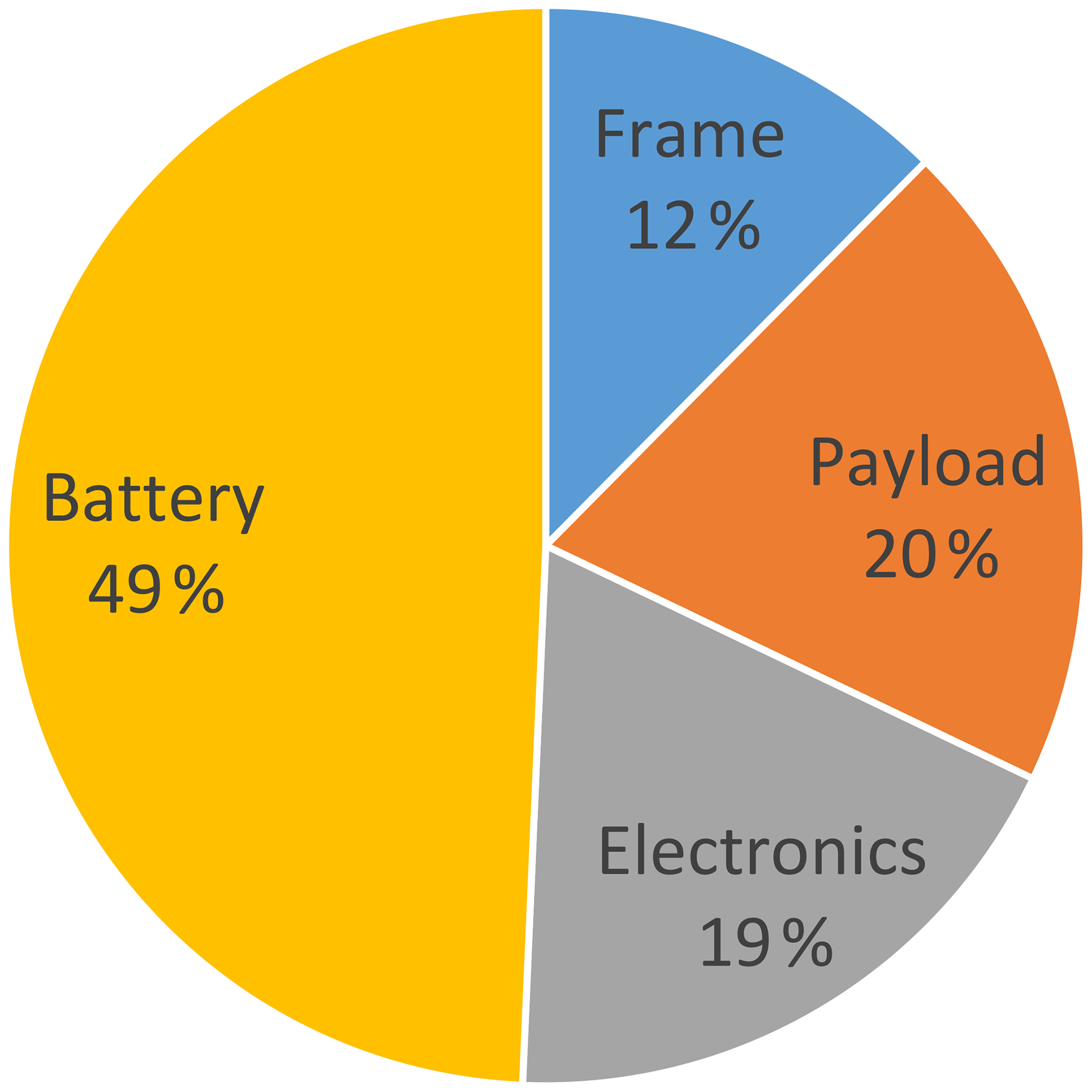
The drone was composed from COTS electronic components and a custom frame. The aim was to achieve the maximum flight time for the specified sensor payloads while keeping a total weight below 5 kg (see Fig. 2). The design was based on calculations using available motor and propeller performance data from different manufacturers. After several iterations, suitable propellers and motors were found, frame weight and payload weight could be determined and refined using preliminary computer-aided design (CAD) drawings. A suitable battery that maximizes flight time but keeps the weight below 5 kg was finally selected. The frame consists of wound carbon fibre tubes and sandwich carbon sheets with balsa end grain core and some 3-D printed covers. See the data sheet (see the data availability section) for detailed information on all the components that were used.
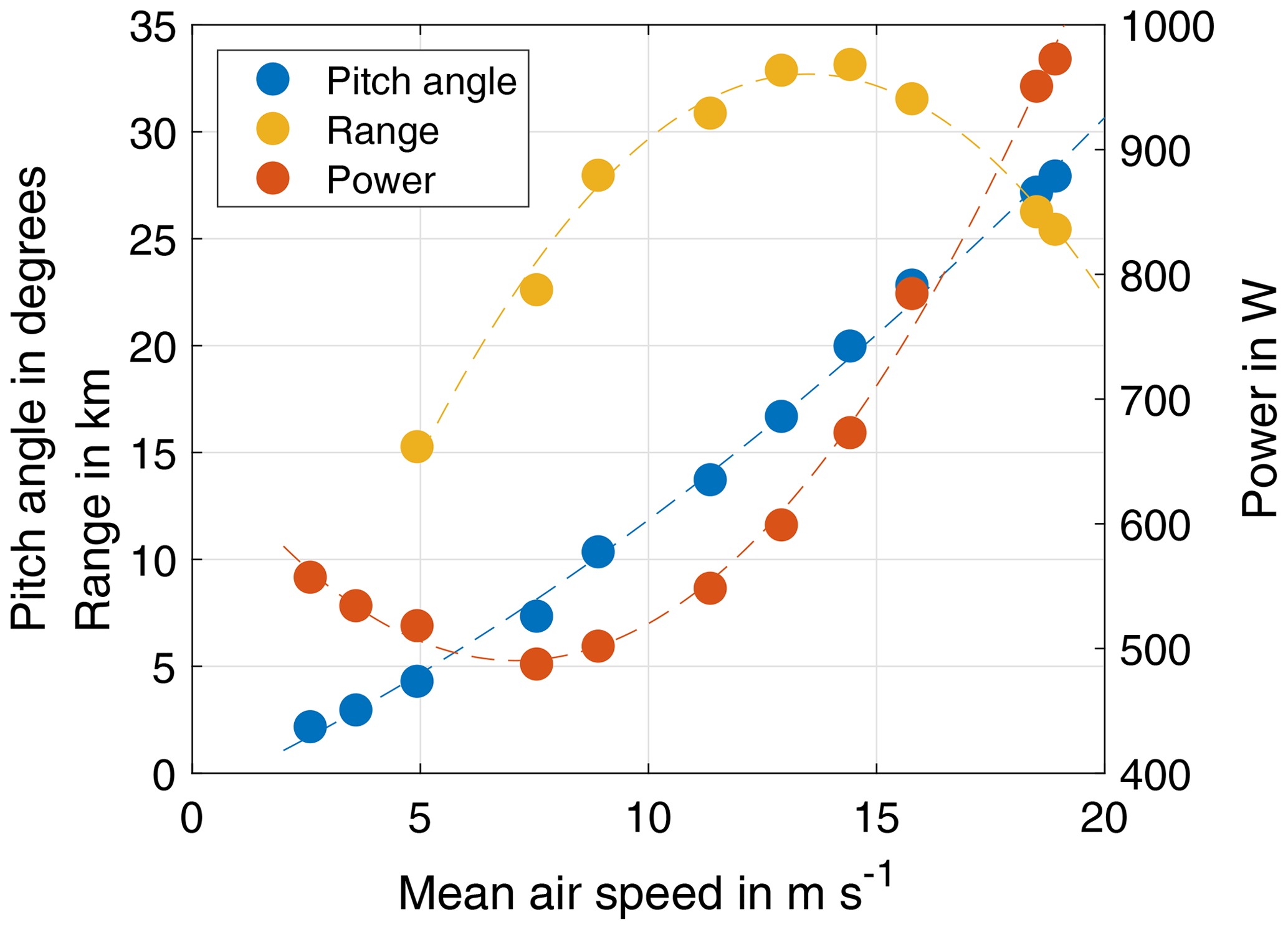
Air speeds of up to 20 m s−1 have been successfully tested in flight. The relation between air speed, pitch angle and power consumption has been determined for the drone (including Gill WindMaster as shown in Fig. 3) by automatically flying circles (D=300 m) at ground speeds between 2 and 18 m s−1, while logging inertial measurement unit (IMU) data with 10 Hz. The relation between air speed and pitch angle is shown in Fig. 4. A pitch angle of 30∘ is not exceeded in normal forward flight. The power consumption has a minimum at 7 m s−1. With a 444 Wh battery, a theoretical maximum flight time of 54 min can be achieved. In practice, only 85 % of the stored energy should be used for safety and battery lifetime reasons, which results in 46 min flight time. When measuring at remote locations and/or at high altitude, a significant portion of the flight time is spent on reaching the measurement location. Therefore, a long flight time is beneficial, as a larger fraction of the total endurance can be spent for acquiring wind speed at the desired location. This allows for longer averaging intervals and/or more measurement locations in a single flight. Significantly less time for swapping batteries is spent during long measurement campaigns. Additionally, the drone is equipped with a dual power supply. Batteries can be swapped without cutting power of the drone, so no reboot or Global Navigation Satellite System (GNSS) reacquisition is required.
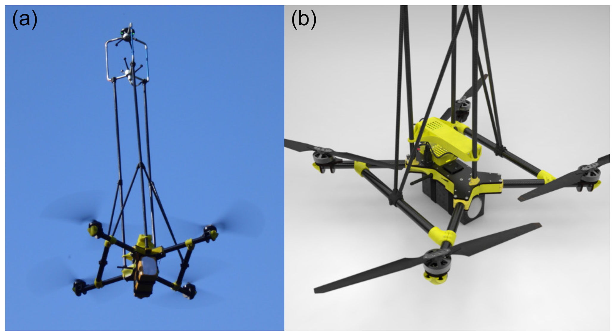
Figure 3(a) The OPTOkopter drone with a Gill WindMaster on a 1 m long mount during a measurement flight. (b) Rendering of the CAD model.
2.3 Anemometer data fusion with UAV speed, attitude and (angular) velocity
Wind speed can be derived from the sum of the relative wind vector (as measured by the sonic anemometer) and the ground speed vector (as measured by the UAV). The UAV uses ArduPilot's extended Kalman filter estimation system (EKF2; Pittelkau, 2003, ardupilot.org) which estimates vehicle position, velocity and angular orientation based on gyroscopes, accelerometer, magnetometer, GNSS, barometer and ground distance measurements.
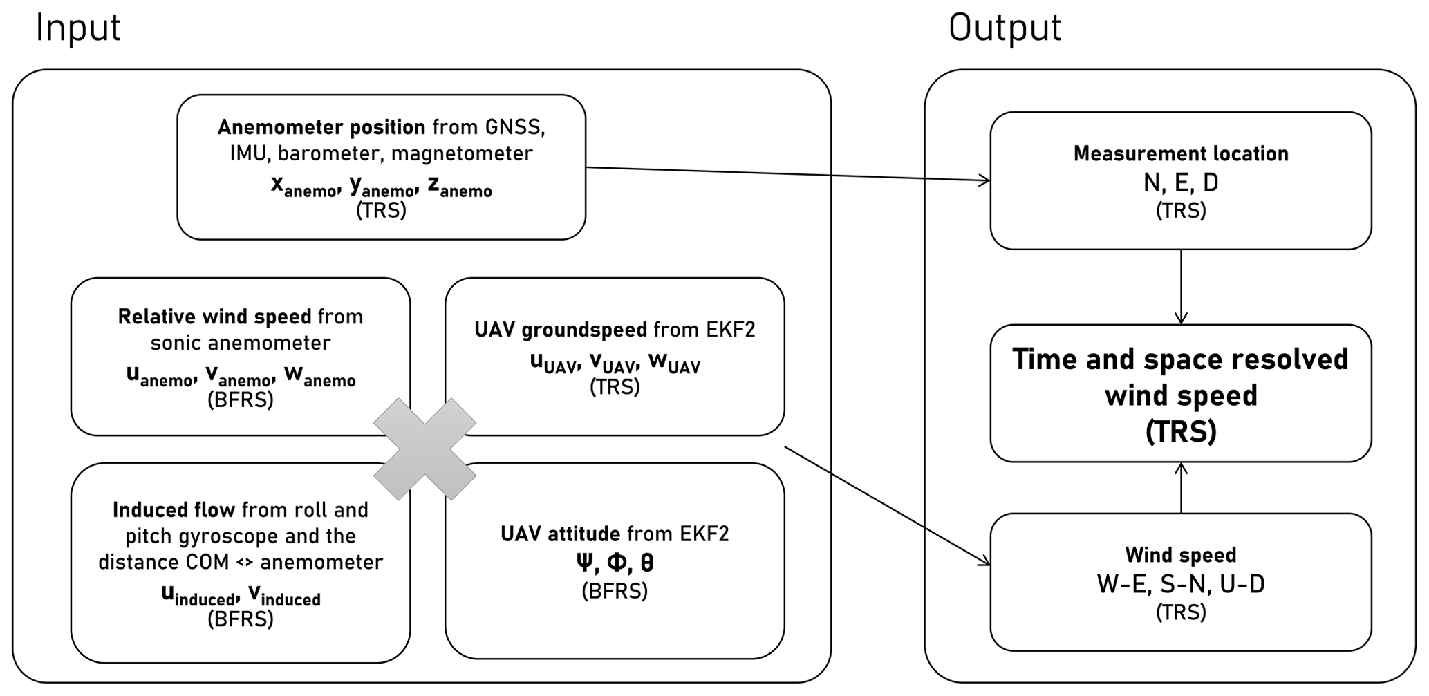
Figure 5Data fusion of sonic anemometry and UAV attitude, position and ground speed. xanemo, yanemo and zanemo are the positions of the anemometer in terrestrial reference system (TRS). uanemo, vanemo and wanemo are the relative wind speeds as measured by the anemometer in body-fixed reference system (BFRS). uUAV, vUAV and wUAV are the ground speeds of the UAV as reported by the EKF2 in TRS. uinduced and vinduced are the induced flow velocities at the measurement volume of the anemometer (lever arm multiplied by angular velocity) for pitch and roll. ψ,ϕ and θ are the attitudes of the UAV as reported by the EKF2 in BFRS. The fusion of the data yields the measurement location in north, east and down (N, E, D; TRS) and the wind speed in west–east, south–north, up–down (W–E, S–N, U–D; TRS) directions.
Wind speed is transformed from a body-fixed reference system (BFRS) to the terrestrial reference system (TRS) using standard rotation matrices. The airflow induced by angular velocities in roll and pitch of the UAV is also compensated for. The input and output data for this transformation are given in Fig. 5. All these calculations are performed on an onboard computer (Raspberry Pi 3B+) that receives wind speed data from the sonic anemometer at 16 Hz and attitude, position and ground speed information from the flight controller of the UAV at 10 Hz. The onboard computer stores the measurement location in the north, east and down terrestrial reference system. The wind speed vector is stored in an west–east, south–north, up–down terrestrial reference system.
3.1 3-D wind sensing performance of sonic anemometers
A miniature sonic anemometer (TriSonica Mini Wind and Weather Sensor; Anemoment, 2020) and a full-size sonic anemometer (factory-precalibrated WindMaster; Gill Instruments Limited, 2020) were tested at 0–360∘ yaw with 0, 10, 20 and 30∘ pitch angles (see Figs. 6 and 7) in a traceable wind tunnel (400 × 260 mm cross section, 400 mm length; accredited according to ISO/IEC 17025, Eidgenössisches Institut für Metrologie (METAS), Switzerland) at wind speeds between . The measurements were compared with a calibrated propeller anemometer (measurement uncertainty 2 %) at 20∘C, 950 hPa and 47 % humidity. Both anemometers were mounted in the wind tunnel using the same attachments as in the drone, including GNSS and/or magnetometer and cable connections to assure that measurement conditions reflect the real situation on the flying drone.
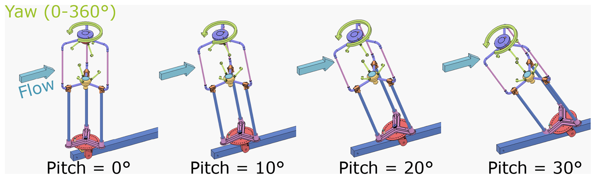
Figure 6Wind tunnel tests of the 3-D wind sensing capabilities. Rotation around the yaw axis (green arrow) for four different pitch angles (from left to right: 0, 10, 20 and 30∘). Wind is coming from the left (blue arrow). A GNSS receiver is mounted on top of the anemometer.
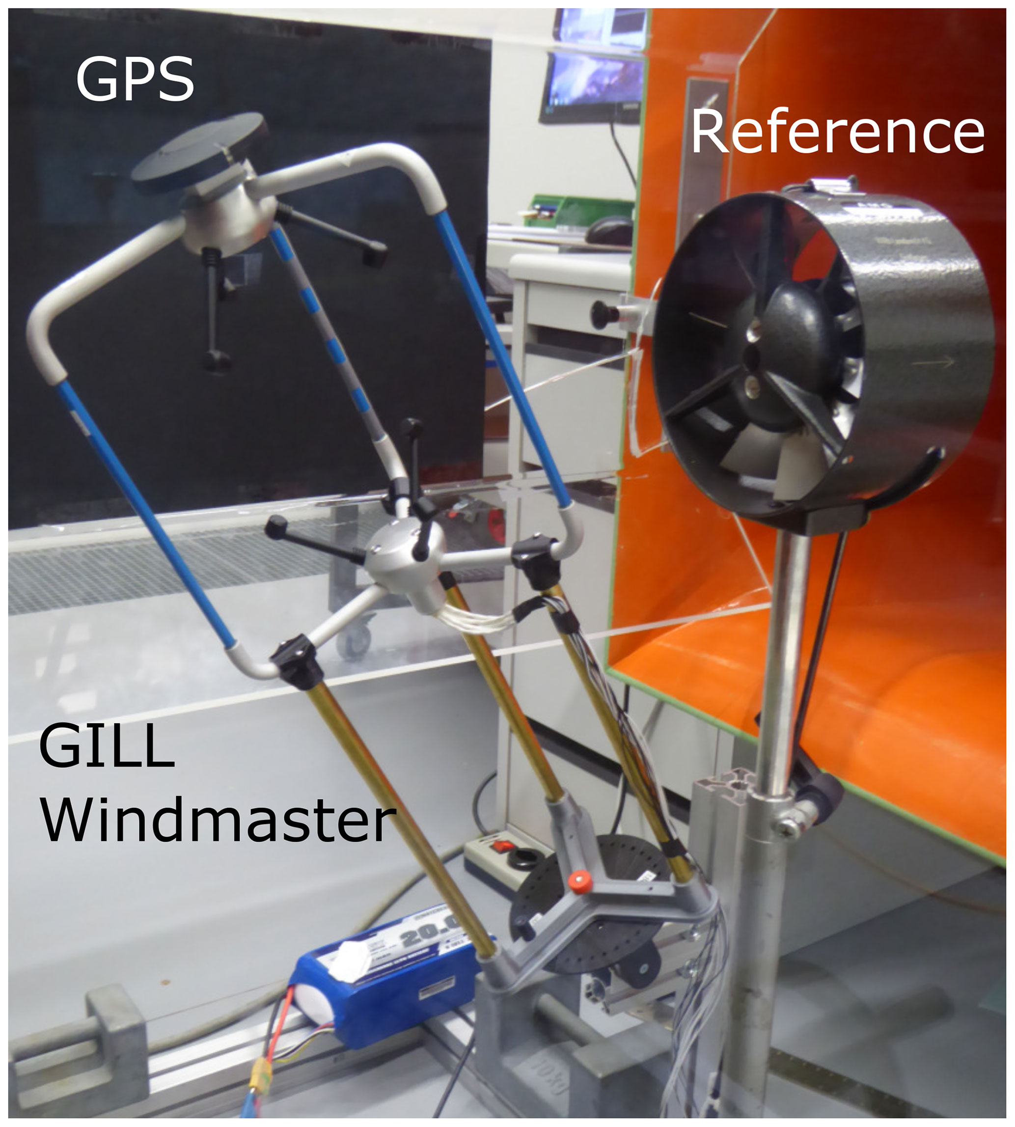
Figure 7Setup of the experiment in the calibration wind tunnel of METAS. The flow is from left to right.
A suitable anemometer for application on UAVs should be able to accurately sense wind speed, azimuth and elevation. This should be possible for all pitch, roll and yaw angles that occur during a typical measurement flight of the UAV. In the proposed design, the maximum pitch angle of the UAV at the maximum air speed (20 m s−1) is 30∘.
Wind speed measurements with the TriSonica are lower than the reference (see Table 1). Note that the results in Table 1 show bias and RMSE for measurements at 15 m s−1 and 0–360∘ yaw angle at four different pitch angles. At large pitch angles there is a strong bias (−17.3 % with a RMSE of 16.2 %). At zero pitch, there still is a bias of −6.3 % and a RMSE of 5.4 %. For the TriSonica, no relation between pitch angle and elevation could be determined. The TriSonica was tested in the wind tunnel in November 2018. After these results were reported to the manufacturer, a firmware update (v 1.7.0, February 2019) addressed the issue of wind shadowing, potentially enhancing the accuracy at zero pitch angle. We had no opportunity to test this firmware in a wind tunnel yet. The issue at higher pitch angles will most likely remain, as we think it is impossible to accurately measure a vertical wind component with a small device with an inherently high blockage ratio. The latest firmware still needs to be tested in a wind tunnel for 0–360∘ and several pitch angles to check for improvements in accuracy. Based on these measurements, we think that the accuracy of 3-D wind measurements with hard-mounted miniature sonic anemometers on UAVs is limited and might explain the limited accuracy that several studies report for in-flight measurements with these kinds of sensors (see the introduction). Miniature sensors should be mounted on a stabilizing gimbal and with the UAV flying at constant altitude to ensure that the vertical wind component is kept low.
Table 1Wind tunnel test. Accuracy of a miniature sonic anemometer (TriSonica) and a full-size sonic anemometer (WindMaster). Each pitch angle was tested with 0–360∘ yaw rotation at 15 m s−1 wind speed. Bias and RMSE are based on the measurements of a full yaw rotation.
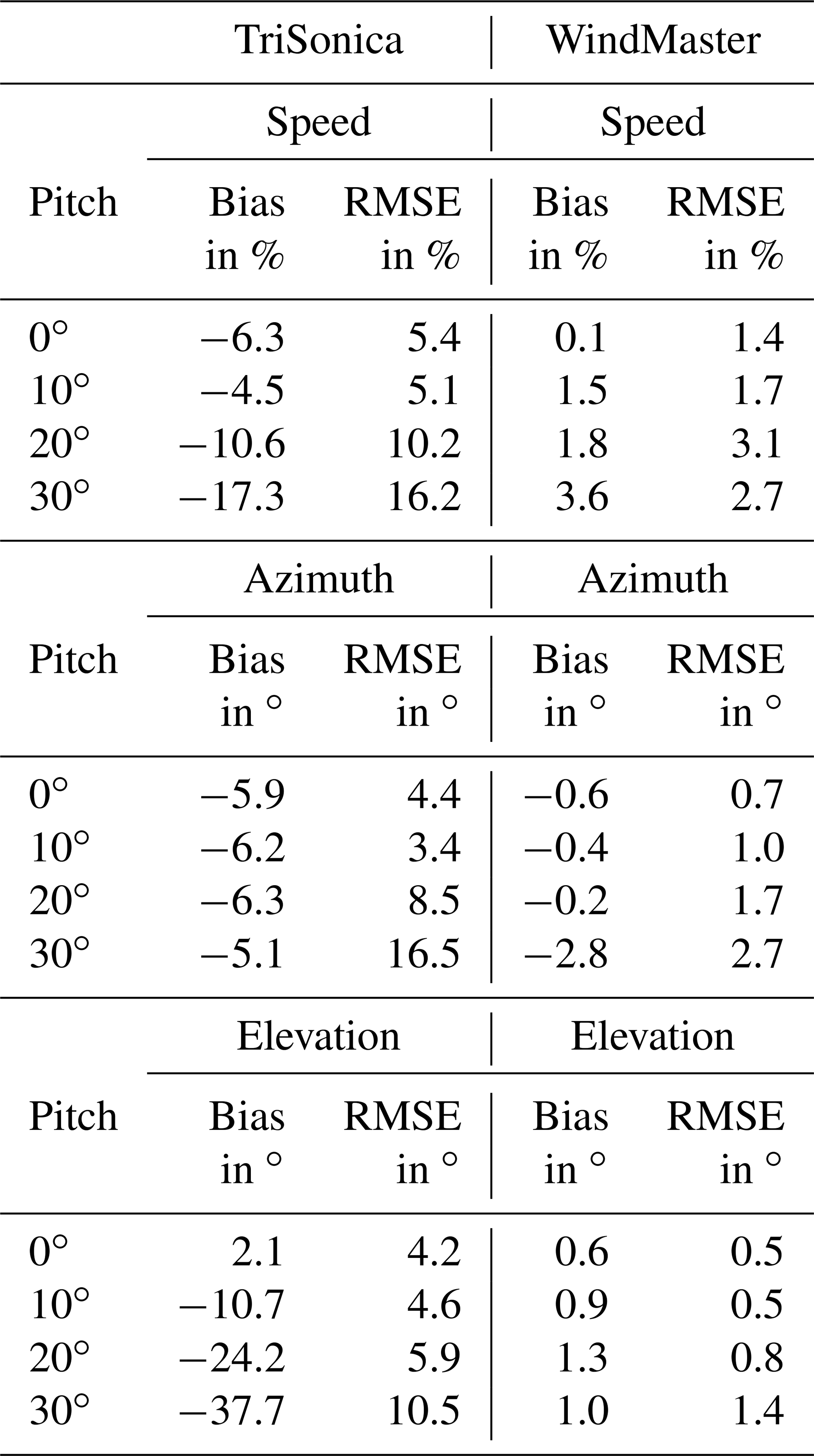
The wind tunnel measurements of the Gill WindMaster anemometer show that bias and RMSE are small, but wind speed is overestimated by up to 3.6 % at 30∘ pitch (see Table 1). Wind azimuth sensing of the WindMaster is almost by a factor of 10 more accurate than in the TriSonica for both bias and RMSE. The WindMaster has a particularly good performance in sensing the wind elevation with a maximum bias of 1.3 and 1.4∘ RMSE. The accuracy of this full-size sonic anemometer is well within the specs given by the manufacturer. Although it weighs by a factor of 20 more than the miniature sensor, we believe that the full-size anemometer is a more suitable instrument for the highly 3-D flow on a flying and manoeuvring non-stationary UAV. This study therefore focuses on in-flight measurements with the Gill WindMaster full-size sonic anemometer.
3.2 Influence of the propeller-induced flow
An anemometer that is mounted on a rotary-wing UAV is potentially measuring a velocity component that is induced by the propellers. It therefore potentially measures a biased wind speed and a biased elevation. The induced component most likely depends on the forward flight speed (air speed in this case). In normal free flight, every flight speed requires a certain pitch angle and propeller speed. Therefore, suitable pitch angles and throttle values (voltage sag compensated) for front and rear motors were determined by flying circles (D=300 m) at different speeds while sampling pitch angle and motor throttle at 10 Hz (see Fig. 8). These data were used for measurements in the wind tunnel of the Technische Universität Dresden (open test section, diameter of 3 m). The drone was fixed to a rigid mount during most of the measurements, but using the data from normal outside free flight allowed us to set realistic motor throttles and pitch angles for each wind tunnel speed. Wind speeds between 1 and 19 m s−1 were tested with the OPTOkopter being tethered to a variable pitch mount. The Gill WindMaster was used as a wind-measuring device on the drone (see Fig. 9). The drone was also flown freely inside the wind tunnel to validate that the mount did not influence the measurements. This test confirmed that motor throttles and pitch angle during free wind tunnel flight and during free outside flight were in close agreement.
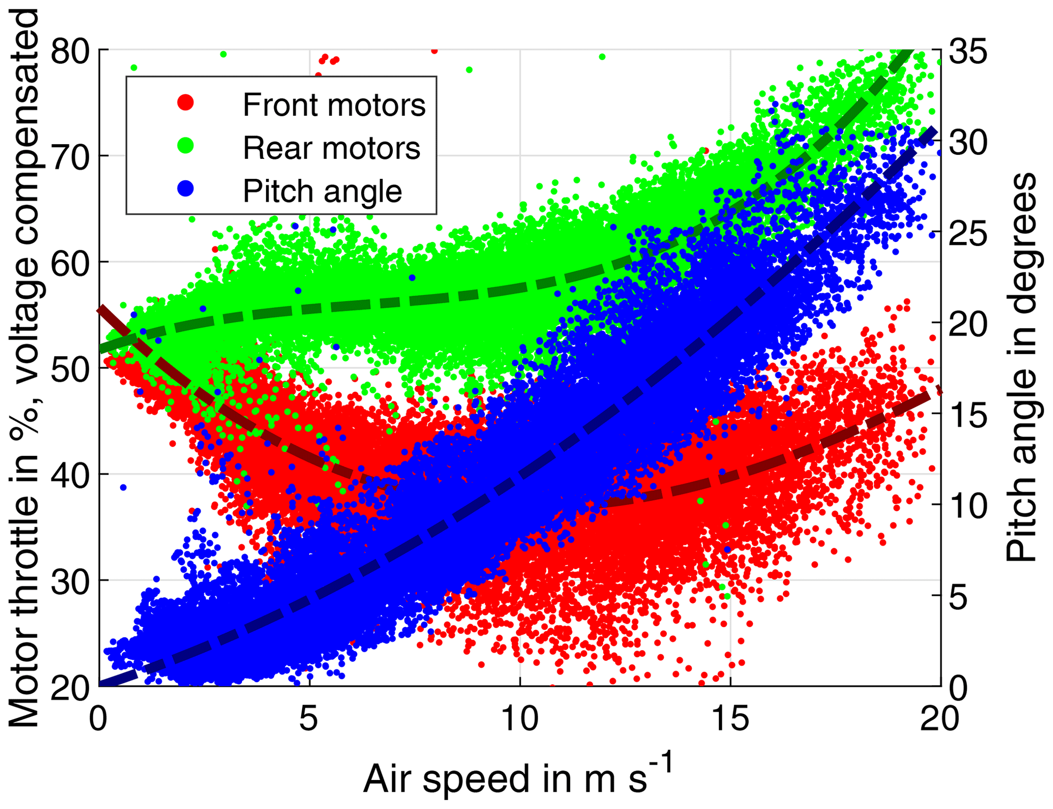
Figure 8Motor throttle (front and rear motor pairs) and pitch angle vs. flight speed. The spread can be explained by the control loops working against external disturbances during free flight in windy conditions. Rear motors generally need to provide more thrust than the front motors to compensate for a pitch-up moment. This effect results from a combination of uneven lift distribution of the rotors in forward flight and gyroscopic precession (US Department of Transportation, 2019). The additional drag of the sonic anemometer amplifies the pitch-up moment which is compensated by higher throttle on the rear motors.
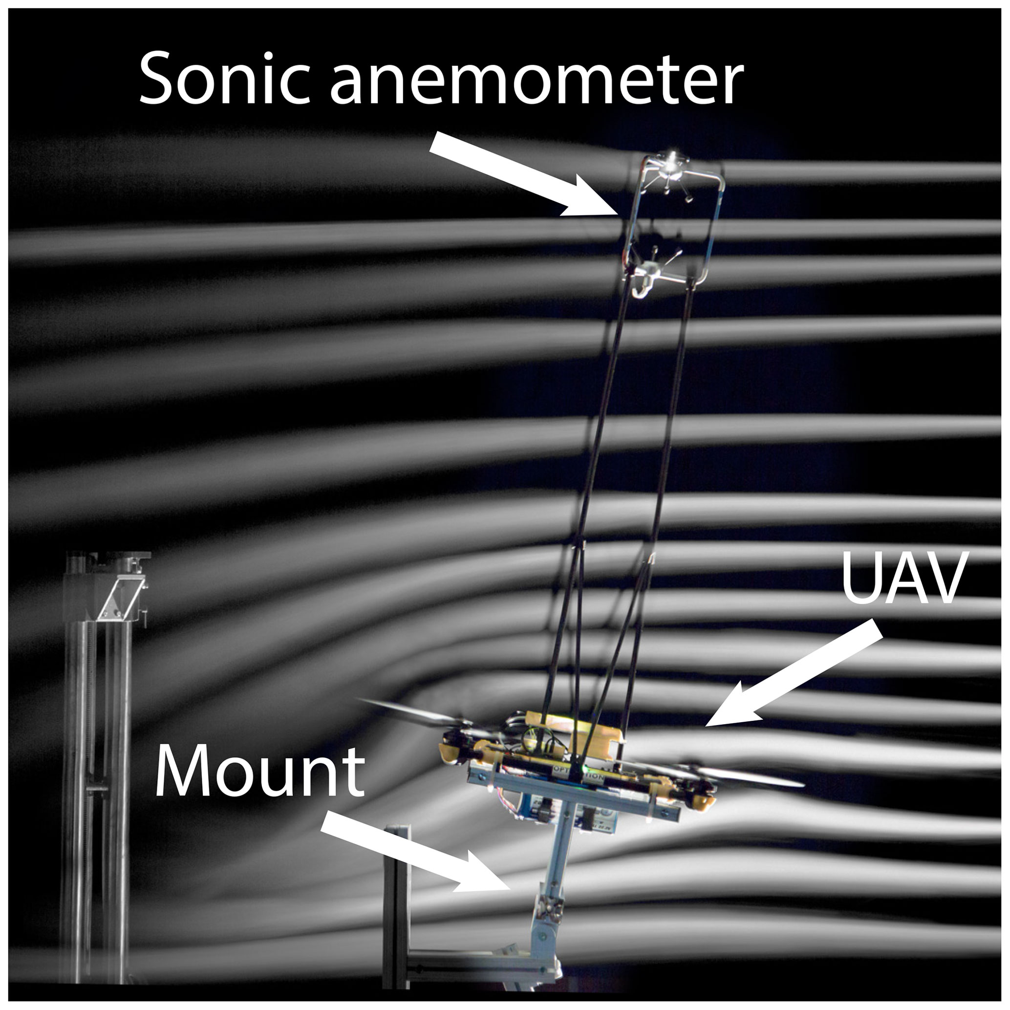
Figure 9Setup of the wind tunnel measurement. The UAV is attached to a mount at multiple suitable pitch angles (here 10∘) representing forward flight. Wind speed measurements (here 9 m s−1) with running motors were compared to measurements with stopped motors. This “tethered” setup was also compared to free flights in the wind tunnel. Smoke trails were used for illustration purposes. A video of the wind tunnel testing is available at https://youtu.be/wWPY3eVxUkU (last access: 9 February 2021).
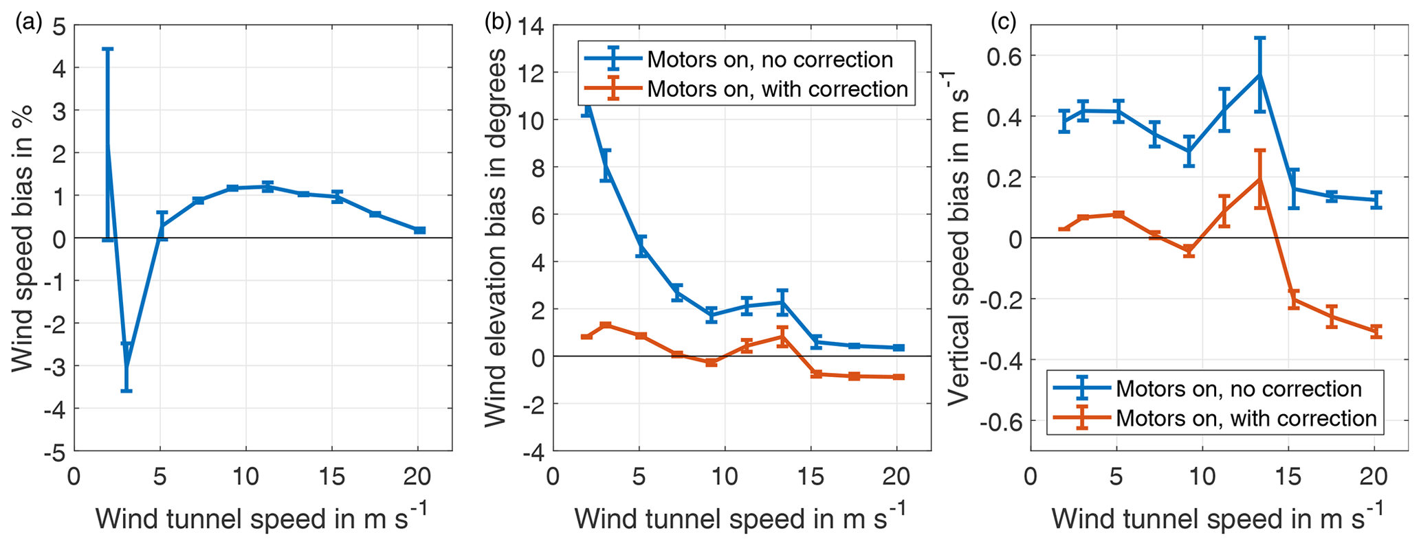
Figure 10Bias of wind speed (a), elevation (b) and vertical speed (c) measurements with running motors, tested in a large wind tunnel. Wind speed measurements with stopped motors are used as a reference. Wind speed bias is ≤ 1 % for wind speeds above 5 m s−1. A simple correction algorithm limits the elevation bias to ≤ 1∘, and the vertical speed bias to ≤ 0.3 m s−1, even at very high wind tunnel speed.
Only little effect of the propeller flow on the measured wind speed was found (see Fig. 10a). The wind speed bias is smaller than 1.5 % for wind speeds above 5 m s−1. The story is different for the wind elevation and the vertical speed. Here, the propeller-induced flow has a large effect for wind speeds ≤ 10 m s−1 (see Fig. 10b and c). The wind elevation bias at very low wind speeds reaches 11∘, and the vertical speed bias is around 0.4 m s−1. This is remarkable, because in comparison to previous studies (see the introduction), the OPTOkopter has a large distance between the anemometer and the propeller discs (1.15 m is the equivalent of 2.5 rotor diameters). The effect diminishes with increasing air speed, however. This propeller-induced flow is compensated for using , where vvertical is the vertical velocity component (in TRS); t is the average motor throttle in percent. The method keeps the bias of wind elevation below 1∘ and the bias of the vertical wind below 0.3 m s−1. The effect of the compensation method is also shown in Fig. 10. To conclude, the propellers impact the direction of the flow (air is deviated downwards, which can be effectively compensated), but there is only a small influence (about 1 %) on the horizontal speed of the air, even at high pitch angles.
3.3 Crosstalk between ground speed, air speed and wind speed
After testing the performance of individual components in the measurement system, the accuracy of the full flying setup (OPTOkopter with Gill WindMaster and all compensations running) was assessed. As mentioned in the introduction, Nichols et al. (2017) report that periodic signals in the wind estimation can often be seen when a UAV is flying periodic manoeuvres and data fusion is imperfect. We checked for such problems by rapidly flying the UAV between two points that were 10 m apart in the east–west direction with a sinusoidal ground speed peaking at about 4 m s−1. Ground speed (as reported by the flight controller), air speed (as reported by the anemometer) and wind speed (as reported by the data fusion) was recorded and converted to the frequency domain using fast Fourier transform. Comparing the amplitude spectrum allows for evaluating the crosstalk between ground speed measurements and wind speed measurements.
In a situation with zero wind, air speed and ground speed as measured by the UAV must be identical. When there is wind, these velocities will not be identical anymore. But any change in ground speed will also result in a change in air speed; hence, a spectral analysis should show peaks at the same frequencies. This is the case in the test flight (see Fig. 11): both air and ground speed have a peak at 0.104 Hz. This is the frequency that the OPTOkopter was oscillating between two waypoints. A linear regression for ground speed and air speed yields a Pearson correlation coefficient of 0.944, indicating that ground speed closely relates to air speed during flight.

Figure 11Amplitude spectrum of ground speed (as reported by the EKF2 in the flight controller), air speed (as reported by the sonic anemometer) and wind speed (as calculated by the data fusion) during a flight where the UAV was repeatedly oscillating in the east–west direction between two waypoints. There is a clear peak at 0.104 Hz in ground speed and air speed (which corresponds to the oscillation between waypoints) but a less distinctive peak in wind speed. This indicates that the effects on wind speed measurements caused by translation and rotation of the UAV are suppressed by a factor of 13.4 by the data fusion.
The FFT analysis (see Fig. 11) reveals that the amplitude spectrum of wind speed at the relevant frequency (0.104 Hz) is about an order of magnitude smaller than air speed or wind speed. Additionally, the correlation coefficient for ground speed and wind speed is 0.164, indicating that there is no relevant linear relationship between these variables. These analyses indicate that the fusion algorithm results in a wind speed measurement that is mostly independent of ground speed and UAV motion/rotation in general. This is very important for airborne measurement systems that do not only perform point measurements in hovering flight but are also capable of measuring while flying a mission. Such a measurement is presented in Sect. 4.
3.4 Comparison with a bistatic lidar
We compared the drone wind measurements with the bistatic Doppler lidar, developed at the Physikalisch-Technische Bundesanstalt (PTB) in Braunschweig, Germany (Oertel et al., 2019; Mauder et al., 2020). A data output rate of 10 Hz was used in the PTB lidar, and different heights between 20 and 100 m were tested.
The bistatic lidar has a small, stationary measurement volume. The distance between the measurement volumes of the OPTOkopter and the lidar was difficult to assess as there was no optical reference that could help with relative positioning as the exact measurement position of the lidar is not visible. However, attempting to fly close to this volume is relatively safe if optical instruments on the UAV such as distance finders and cameras are isolated from the high laser power.
After performing several flights, we selected a measurement at 40 m height for a detailed analysis, as the correlation between wind speed measurements of the two methods was maximal for this dataset, indicating that we were flying very close to the measurement volume of the PTB lidar. We compared the data of the lidar reference to the drone measurement using an orthogonal Deming regression. RMSE and bias (based on paired observations) were determined for all measurement flights.
The OPTOkopter was always hovering at the lee side of the measurement volume. Wind speed, azimuth and elevation were sampled during multiple short flights of 10 min. Additionally, we were measuring wind speeds while circling (4 m radius, 2.5 m s−1 flight speed) around the lidar measurement volume to check for non-zero ground-speed-related errors (see Fig. 12).

Figure 12Measurement site of the PTB lidar reference. This 3-D model of the location was calculated using photogrammetry with image data that were captured during the wind measurement flights.

Figure 13Wind speed (a), azimuth (b) and elevation (c) measurements at 10 Hz, with comparison of measurement from the PTB lidar with the OPTOkopter at 40 m height. Wind speed varies between 1.5 and 9.5 m s−1. Wind azimuth varies between 200 and 300∘. Wind elevation varies between −42 and +25∘.
The measurement volume of the lidar at 40 m height is surrounded by tall buildings and trees, generating highly unsteady flow: the wind speed varies by 8 m s−1, the azimuth by about 100∘ and the elevation by about 67∘ during this selected measurement flight (see Fig. 13). These numbers emphasize the importance of being capable to measure three-dimensional wind with a suitable anemometer. Despite the dynamic situation, the comparison with the PTB lidar reference shows an excellent agreement of the three-dimensional wind speed (see Fig. 13). Note that these figures show measurements that were taken with 10 Hz sampling rate.
A linear Deming regression of the data in 1 s averaging intervals has a slope of 1.03 and an offset of −0.03. The correlation coefficient is 0.95, indicating a good linear relation between both methods (see Fig. 14). We also analysed the effect of increasing averaging intervals (between 0.1 and 100 s) on bias and RMSE. As expected, bias does hardly change when the averaging interval is increased. For the wind speed measurement, bias is between 2.9 % and 3.7 %, which is very similar to what was determined for the isolated WindMaster in the calibration wind tunnel (see Table 1). The wind speed RMSE is strongly dependent on averaging interval: it drops from 12 % at 0.1 s to 1 % at 100 s (see Fig. 15a).
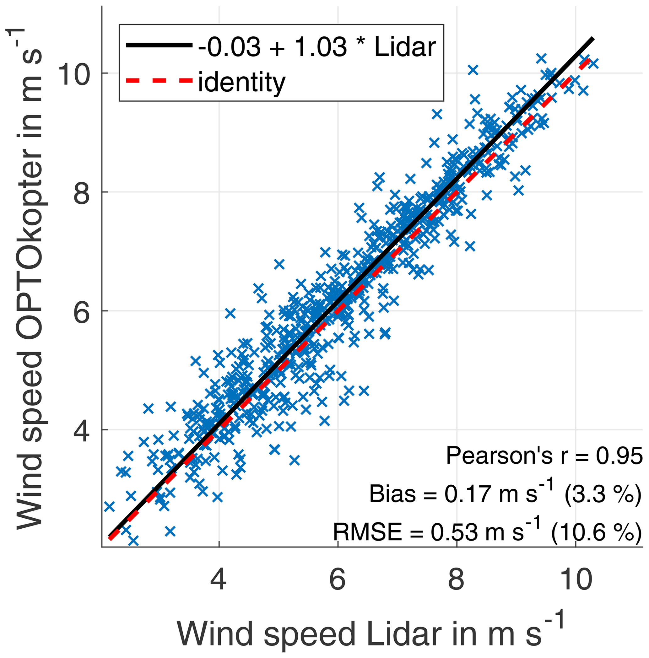
Figure 14Linear Deming regression of the UAV wind speed measurement at 40 m height for 1 s averaging interval. The PTB lidar is used as a reference instrument.
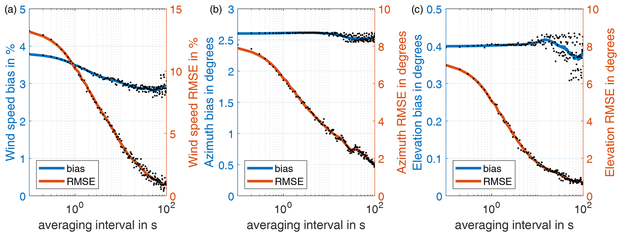
Figure 15Bias and RMSE of the UAV wind speed (a), azimuth (b) and elevation (c) measurements at 40 m height for averaging intervals between 0.1 s (10 Hz) and 100 s (0.01 Hz). The PTB lidar is used as a reference instrument.
The azimuth has a constant bias of about 2.6∘ and a RMSE decreasing from 7 to 1.9∘ (see Fig. 15b). The offset can result from a misalignment of the lidar, or interference of the compass on the UAV. We believe that this uncertainty is acceptable. It could be improved by fusing the heading measurements of the UAV with additional sensors like dual real-time kinematic (RTK) GPS rovers. The elevation bias is constantly at about 0.4∘. RMSE decreases from 7∘ at 0.1 s averaging interval to 1∘ at 100 s (see Fig. 15c).
Bistatic lidar and OPTOkopter hence give closely matched results, even at 10 Hz sampling interval. Naturally, this consistency increases with longer averaging intervals. When measuring at slightly different locations, the influence of spatial and temporal wind speed differences decreases with longer averaging intervals, lowering RMSE. Long averaging intervals also reduce measurement noise of both methods, again decreasing RMSE.
Turbulence intensity (TI; averaging interval of 10 s) decreases with altitude (e.g. Svensson et al., 2019). Despite a short sampling time per height (10 min) we also find this relation in our measurements (Pearson's r of −0.79, we take the average of TILidar and TIUAV to approximate the true TI). A significant linear correlation was found also for turbulence intensity and wind speed RMSE (r of 0.76), azimuth RMSE (r of 0.90) and elevation RMSE (r of 0.87). As a matter of course, the measured TI also decreases when the averaging interval is increased, yielding lower RMSE (see Fig. 15). A large distance between the measurement volumes, together with a high TI, will therefore result in high RMSE.
Despite sometimes flying very close to the lidar, we believe that the presence of the UAV did not significantly change the flow in the measurement volume of the lidar: the measurements of the OPTOkopter have been successfully compensated for propeller-induced flow (see Fig. 10). If the OPTOkopter would have changed the vertical flow component in the measurement volume of the lidar, then there would be a large discrepancy between (compensated) OPTOkopter measurement and (uncompensated) lidar measurement. The relative position of the OPTOkopter to the measurement volume of the lidar changed significantly while we were flying circles around the lidar. If there would be a significant influence from the OPTOkopter, then this should be visible as periodic bias error, but this has not been observed in the data.
The wind turbine (Enercon E 70–E 4) is located in the Black Forest in southern Germany (47∘45′53.43′′ N; 007∘51′11.68′′ E) at about 1012 m above sea level. The nacelle height is 85 m and the rotor diameter (D) is 71 m (see Fig. 16). Wind velocity was determined at 2D behind the rotor disc. Flight duration was 22 min, and measurements were taken at 16 Hz. The OPTOkopter was oscillating at constant altitude at nacelle height with a velocity of 5 m s−1 on a path parallel to the rotor disc (see Figs. 16 and 18). Because the wind speed quite substantially varied with time (see Fig. 17), all wind measurements were normalized with the reference anemometer velocity on top of the nacelle (uref). Measurements were discretized in intervals of 1 m along the flight path. Data from each of these bins were averaged.

Figure 16Measurement site of the wind turbine study. (a) The red arrow indicates wind direction. The pink line indicates rotor disc in top view. The dashed cyan line indicates constant altitude flight path of the OPTOkopter. The dashed yellow line indicates the path for the elevation profile shown in the middle (image taken from © Google Earth). (b) Elevation profile of the measurement site. (c) Photograph of the wind turbine in the Black Forest.
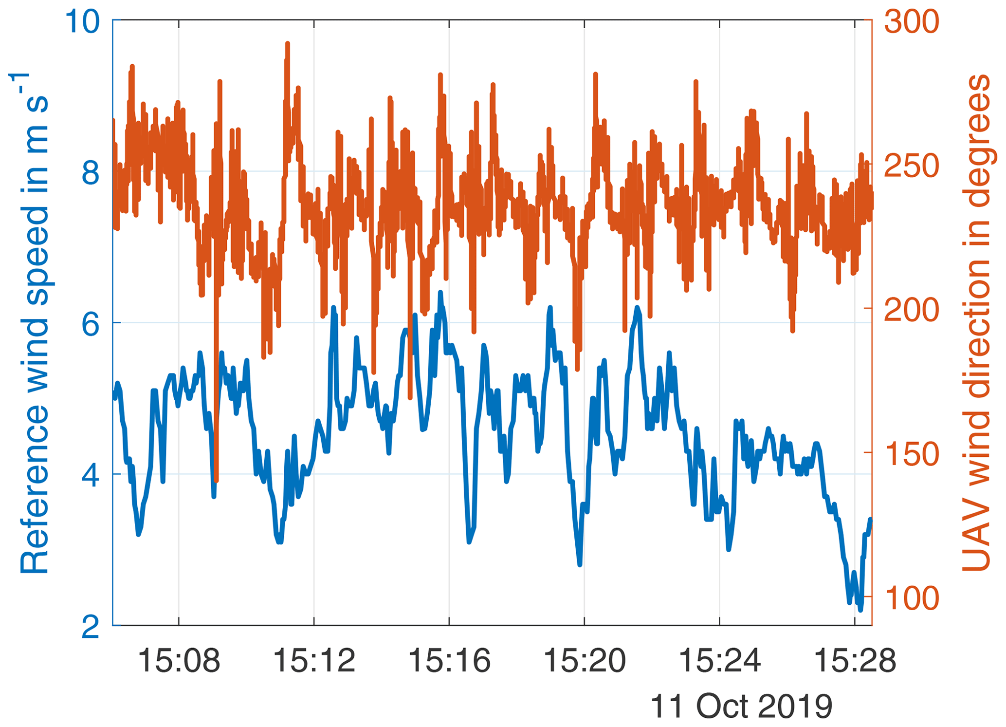
Figure 17Wind speed and wind direction during the measurement flight. Wind speed was measured by the reference cup anemometer on top of the nacelle uref. Wind speed varied between 2.1 and 6.5 m s−1. No reference sensor was available for wind direction; hence, the figure shows wind direction as measured by the UAV (including all variations introduced by the wind turbine rotor). Wind direction varied between 140 and 290∘.

Figure 18Flight path of the OPTOkopter behind the wind turbine (view from the front). The drone oscillates with 5 m s−1 between waypoints W1 and W2.
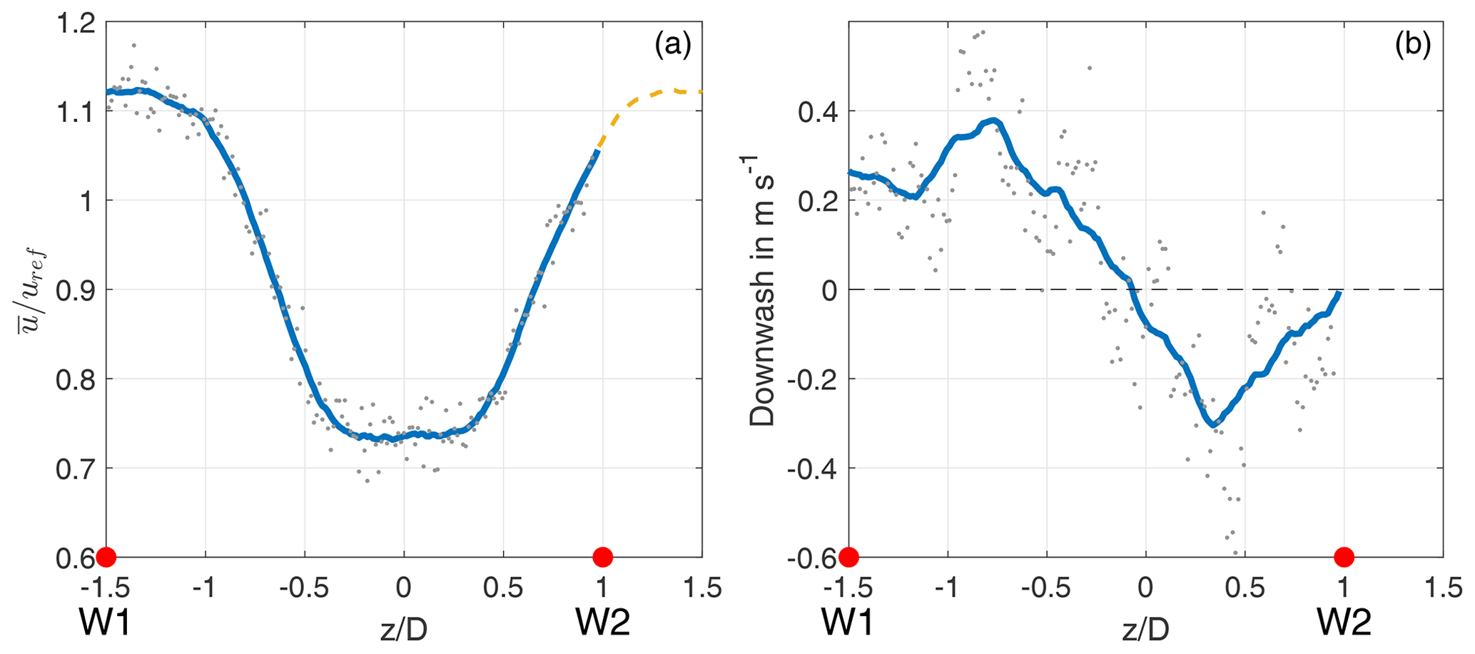
Figure 19Horizontal cross section at nacelle height through the wake of a wind turbine. (a) Points indicate discretized wind velocity measurements. The line indicates smoothed data (Savitzky–Golay filter). The dashed yellow line indicates missing data. A velocity deficit behind the rotor is clearly visible. (b) Points indicate discretized downwash velocity measurements. The line indicates smoothed data (moving mean). Swirl results in downwash on the left side and upwash on the right side in the wake of the wind turbine.
A relatively constant velocity deficit () of 25 % is found behind the full diameter of the rotor disc. Further away from the rotor tips, the velocity becomes even larger than uref (see Fig. 19). Most likely, the reference anemometer is measuring velocities lower than the true free-stream velocity, due to the proximity to the nacelle, and possible shadowing effects by the rotor blades. When a wind turbine rotates clockwise (as viewed from the front), it will generate a swirl with anti-clockwise rotation. In a horizontal cross section at nacelle height, this will result in air travelling down on the left side (again viewed from the front) and air travelling up on the right side. The swirl was captured (see Fig. 19, right), the magnitude is about 0.35 m s−1, which is about 7.7 % of the average free-stream velocity. The downwash is not perfectly symmetric around the centre of the wind turbine and may be influenced by the slope behind the wind turbine (see Fig. 16, middle).
Data at were not captured, as the wind direction slightly changed after the waypoints were positioned and uploaded to the UAV. The results of the measurements are strikingly similar to theoretical velocity distributions (e.g. Wu and Porté-Agel, 2012; Keane et al., 2016) and lidar measurements in the wake of wind turbines (e.g. Vollmer et al., 2017; Menke et al., 2018). The noise in the measurements most likely results from the inconsistent free-stream velocity (see Fig. 17) and can presumably be decreased significantly by measuring for a longer duration (e.g. using more than one battery pack).
The environmental science of the atmospheric boundary layer benefits from wind speed measurements collected by UAVs. A suitable lightweight rotary-wing UAV was designed for carrying an anemometer. Drones can measure close to structures and they can be validated comfortably by hovering close to a reference instrument. Flight time is often an issue with UAV-based measurements. In the proposed design, the battery is responsible for 49 % of the total weight. It can be replaced by COTS power-tethering devices that allow for much longer, uninterrupted measurement flights at a single location at different altitudes up to 100 m.
The OPTOkopter uses a full-size industry-standard anemometer instead of a miniature version, as the accuracy in three-dimensional flow is better by 1 order of magnitude. Measurements at the test site of the PTB lidar have shown that three-dimensional flow is highly likely to happen in situ, even when the OPTOkopter hovers on spot at a constant altitude. Due to the high contribution of vertical flow, using a single miniature sonic anemometer does not seem to be feasible on a drone, even when the sensor is mounted on a stabilizing gimbal. The performance of an anemometer that is to be installed on a drone should be verified at suitable tilt angles in a precision wind tunnel. The maximum tilt angle needs to be determined with drone test flights at the maximum desired wind speed.
Propeller-induced flow mainly adds a vertical component to the flow without adding a horizontal component – even at large pitch angles. The vertical component can effectively be compensated by subtracting a value that is proportional to the mean motor throttle. Placing the wind sensor far away from the rotors is a key requirement for this simple correction to work. As has been shown in Fig. 9, flow distortion at the sonic anemometer is very small. This ensures that changing the pitch angle of the drone will not change the amount of flow distortion that is present at the anemometer location. In this case, a simple correction for the vertical flow component, which depends only on the average motor throttle, can be used. The gain of this correction should ideally be determined and verified in a large wind tunnel.
Mounting an anemometer on such a long lever arm significantly increases the moment of inertia of the drone. It is therefore necessary to adjust the control loop parameters (e.g. proportional gain (P) of the roll and pitch angular velocity controller was increased by a factor of 4 and derivative gain (D) by a factor of 3). Care has to be taken to mount the anemometer exactly on top of the centre of gravity; otherwise, the roll and pitch motion of the drone results in an additional yaw moment. Yaw control is typically the weakest axis in quadrotors, so this could lead to serious control problems during flight. Furthermore, the anemometer mount needs to be very stiff in roll, pitch and yaw axes; otherwise, oscillations (due to the increased P and D) are very likely to happen.
Table 2Bias and RMSE of the OPTOkopter wind measurements at 10 s averaging interval, with the PTB lidar reference. The table includes data from all flights that were done. The distance to the measurement volume of the lidar was difficult to assess, but it was smaller than 10 m in all cases. The comparison was done with the OPTOkopter hovering on spot or circling around the lidar measurement volume. Wind speed bias is generally low. RMSEs seem to increase with turbulence intensity.
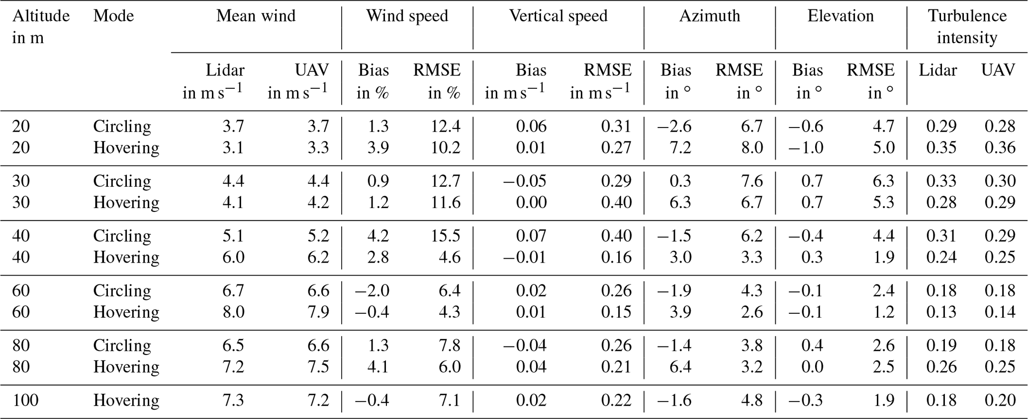
The crosstalk between ground speed and wind speed is suppressed by a factor of 13, although relatively aggressive manoeuvres were flown (oscillating between two waypoints that were only 10 m apart). These results are supported by low bias and RMSE during the comparison with the bistatic lidar in hovering and circling flight mode (see Table 2).
The analysis of the wind velocity in the wake of a wind turbine has proven the practicability of accurate UAV-based measurements. The application is not limited to point measurements. The mean wind speed on a 200 m long path behind the wind turbine rotor has been sampled with 1 m resolution. Such an analysis can be executed in significantly less than an hour including all preparations. The only requirements are a free space of 2 × 2 m for take-off and landing (e.g. the roof of a car), peak wind speeds that do not exceed 20 m s−1, free line of sight between pilot and UAV and preferably no rain.
Based on the tests of the individual components and the full system, we think that mounting the anemometer on the drone does not significantly increase the measurement uncertainty of the anemometer in hovering flight. Wind speed and elevation are sensed accurately, when data fusion is performed as described, and separation between wind sensor and propellers is large enough (here 2.5 rotor diameters). Additionally, the maximum tilt of the drone must not exceed the maximum acceptance angle of the anemometer (30∘ in our case).
There certainly is room for improvement in sensing the azimuth (see Table 2), which is currently limited by the magnetometer. The strongest source of interference usually are the motors of the UAV. This internal interference is effectively limited by mounting the magnetometer at a distance of 1.3 m to the motors. However, external disturbances can occur when flying close to metallic structures, which may still bias the azimuth. More accurate magnetometers recently became available for use in the ArduPilot firmware (e.g. PNI RM3100). Dual RTK GPSs or landmarks on the ground that are captured from the drone are additional possibilities to reduce azimuth bias.
We think that the devices that are designed following the propositions presented in this study are very suitable for accurate wind measurements up to 20 m s−1 and up to 46 min duration. Additional sensors can be attached, e.g. allowing us to trace the sources of pollution automatically, by always flying against the wind vector. Drones like the OPTOkopter, which are specifically designed for the application, might be used as cost-effective, flexible and quickly deployable addition to measurement masts and lidar scans.
Data of all measurements presented in this paper (except for the PTB lidar data) and additional information on the OPTOkopter are available at https://doi.org/10.6084/m9.figshare.12581678.v4 (Thielicke et al., 2020).
WT wrote the manuscript with input from all authors, and developed and operated the OPTOkopter together with WH. UM initiated and supported the development, and assisted with all measurements that are presented. ME constructed the PTB lidar system and its signal processing. PW and ME operated the Doppler lidar and preprocessed its 10 and 1 Hz raw data. All authors contributed to the discussion of the results.
William Thielicke, Waldemar Hübert and Ulrich Müller developed the OPTOkopter while being employed at OPTOLUTION Messtechnik GmbH, a company that is aiming to commercialize measurement services with this drone.
We thank the Technische Universität Dresden, Fakultät Maschinenwesen, Institut für Luft- und Raumfahrttechnik, Experimentelle Aerodynamik and especially Veit Hildebrand for the opportunity to fly inside the wind tunnel. We thank Klaus-Peter Neitzke (Hochschule Nordhausen) and Thomas Eipper (Technische Universität Dresden) for the assistance with measurements and photographs during the wind tunnel flights. We thank the Eidgenössische Institut für Metrologie (METAS) for the opportunity to test the sonic anemometers in their wind tunnel. We thank Erwin Schlauderer at Ökostrom Erzeugung Freiburg GmbH for allowing us to measure the wind turbine wake. We thank the ArduPilot community for developing a safe, great and open flight controller firmware.
This paper was edited by Szymon Malinowski and reviewed by two anonymous referees.
Adkins, K. A., Swinford, C. J., Wambolt, P. D., and Bease, G.: Development of a sensor suite for atmospheric boundary layer measurement with a small multirotor unmanned aerial system, International Journal of Aviation, Aeronautics, and Aerospace, 7, 1–4, https://doi.org/10.15394/ijaaa.2020.1433, 2020. a, b
Anemoment: TriSonica mini wind and weather sensor, Anemoment, available at: https://anemoment.com/features/#trisonica-mini (last access: 9 February 2021), 2020. a
Barbieri, L., Kral, S. T., Bailey, S. C. C., Frazier, A. E., Jacob, J. D., Reuder, J., Brus, D., Chilson, P. B., Crick, C., Detweiler, C., Doddi, A., Elston, J., Foroutan, H., González-Rocha, J., Greene, B. R., Guzman, M. I., Houston, A. L., Islam, A., Kemppinen, O., Lawrence, D., Pillar-Little, E. A., Ross, S. D., Sama, M. P., Schmale, D. G., Schuyler, T. J., Shankar, A., Smith, S. W., Waugh, S., Dixon, C., Borenstein, S., and de Boer, G.: Intercomparison of Small Unmanned Aircraft System (sUAS) Measurements for Atmospheric Science during the LAPSE-RATE Campaign, Sensors, 19, 2179, https://doi.org/10.3390/s19092179, 2019. a, b, c, d
Barthelmie, R. J., Crippa, P., Wang, H., Smith, C. M., Krishnamurthy, R., Choukulkar, A., Calhoun, R., Valyou, D., Marzocca, P., Matthiesen, D., Brown, G., and Pryor, S. C.: 3D wind and turbulence characteristics of the atmospheric boundary layer, B. Am. Meteorol. Soc., 95, 743–756, https://doi.org/10.1175/bams-d-12-00111.1, 2014. a
Bilbro, J., Fichtl, G., Fitzjarrald, D., Krause, M., and Lee, R.: Airborne Doppler Lidar Wind Field Measurements, B. Am. Meteorol. Soc., 65, 348–359, https://doi.org/10.1175/1520-0477(1984)065<0348:adlwfm>2.0.co;2, 1984. a
Bottma, M., Verkaik, J. W., Zwerver, S., van Rompaey, R. S. A. R., Kok, M. T. J., and Berk, M. M.: K-Gill propeller vane observations for the Cabauw parametrization experiment, in: Studies in Environmental Science, 65, 269–274, Elsevier, https://doi.org/10.1016/s0166-1116(06)80210-4, 1995. a
Camp, D. W., Turner, R. E., and Gilchrist, L. P.: Response tests of cup, vane, and propeller wind sensors, J. Geophys. Res., 75, 5265–5270, https://doi.org/10.1029/jc075i027p05265, 1970. a
Christen, A., Van Gorsel, E., Vogt, R., Andretta, M., and Rotach, M.: Ultrasonic anemometer instrumentation at steep slopes-wind tunnel study-field intercomparison-measurements, MAP Newsletter, 15, 164–167, available at: https://ibis.geog.ubc.ca/~achristn/publications/2001/2001-MAP-Christen-et-al.pdf (last access: 9 February 2021), 2001. a
Decagon Devices, Inc: DS-2Sonic Anemometer, Operators Manual, Decagon Devices, Inc, available at: http://manuals.decagon.com/Manuals/14586_DS2_Web.pdf (last access: 9 February 2021), 2017. a
Donnell, G. W., Feight, J. A., Lannan, N., and Jacob, J. D.: Wind characterization using onboard IMU of sUAS, in: 2018 Atmospheric Flight Mechanics Conference, Georgia, 25–29 June 2018, Atlanta, USA, 2986, https://doi.org/10.2514/6.2018-2986, 2018. a, b, c, d, e, f
Elston, J., Argrow, B., Stachura, M., Weibel, D., Lawrence, D., and Pope, D.: Overview of Small Fixed-Wing Unmanned Aircraft for Meteorological Sampling, J. Atmos. Ocean. Tech., 32, 97–115, https://doi.org/10.1175/jtech-d-13-00236.1, 2014. a, b
FT Technologies Ltd.: FT205 lightweight acoustic resonance wind sensor, FT Technologies Ltd., available at: https://fttechnologies.com/wind-sensors/lightweight/ft205/ (last access: 9 February 2021), 2020. a
Gill Instruments Limited: WindMaster 3-Axis Ultrasonic Anemometer, available at: http://gillinstruments.com/data/datasheets/WindMasteriss6.pdf (last access: 9 February 2021), 2020. a
Grare, L., Lenain, L., and Melville, W. K.: The Influence of Wind Direction on Campbell Scientific CSAT3 and Gill R3-50 Sonic Anemometer Measurements, J. Atmos. Ocean. Tech., 33, 2477–2497, https://doi.org/10.1175/jtech-d-16-0055.1, 2016. a
Herges, T. G., Maniaci, D. C., Naughton, B. T., Mikkelsen, T. K., and Sjöholm, M.: High resolution wind turbine wake measurements with a scanning lidar, J. Phys. Conf. Ser., 854, 12021, https://doi.org/10.1088/1742-6596/854/1/012021, 2017. a
Hollenbeck, D., Nunez, G., Christensen, L. E., and Chen, Y.: Wind Measurement and Estimation with Small Unmanned Aerial Systems (sUAS) Using On-Board Mini Ultrasonic Anemometers, International Conference on Unmanned Aircraft Systems (ICUAS), 12–15 June 2018, Dallas, TX, USA, 285–292, https://doi.org/10.1109/icuas.2018.8453418, 2018. a, b
Hutchins, N., Monty, J., Hultmark, M., and Smits, A.: A direct measure of the frequency response of hot-wire anemometers: temporal resolution issues in wall-bounded turbulence, Exp. Fluids, 56, 18, https://doi.org/10.1007/s00348-014-1856-8, 2015. a
Ivey, M., Petty, R., Desilets, D., Verlinde, J., and Ellingson, R.: Polar Research with Unmanned Aircraft and Tethered Balloons, US Department of Energy Office of Science, https://doi.org/10.2172/1226560, 2014. a
Izumi, Y. and Barad, M. L.: Wind Speeds as Measured by Cup and Sonic Anemometers and Influenced by Tower Structure, J. Appl. Meteorol., 9, 851–856, https://doi.org/10.1175/1520-0450(1970)009<0851:wsambc>2.0.co;2, 1970. a
Johansen, T. A., Cristofaro, A., Sørensen, K., Hansen, J. M., and Fossen, T. I.: On estimation of wind velocity, angle-of-attack and sideslip angle of small UAVs using standard sensors, in: 2015 International Conference on Unmanned Aircraft Systems (ICUAS), 9–12 June 2015, Denver, Colorado, USA, 510–519, https://doi.org/10.1109/icuas.2015.7152330, 2015. a
Keane, A., Aguirre, P. E. O., Ferchland, H., Clive, P., and Gallacher, D.: An analytical model for a full wind turbine wake, J. Phys. Conf. Ser., 753, 032039, https://doi.org/10.1088/1742-6596/753/3/032039, 2016. a
Kochendorfer, J., Meyers, T. P., Frank, J., Massman, W. J., and Heuer, M. W.: How well can we measure the vertical wind speed? Implications for fluxes of energy and mass, Bound.-Lay. Meteorol., 145, 383–398, https://doi.org/10.1007/s10546-012-9738-1, 2012. a
Kumer, V.-M., Reuder, J., Svardal, B., Sætre, C., and Eecen, P.: Characterisation of single wind turbine wakes with static and scanning WINTWEX-W LiDAR data, Energy Proced., 80, 245–254, https://doi.org/10.1016/j.egypro.2015.11.428, 2015. a
Labovský, J. and Jelemenský, L.: Verification of CFD pollution dispersion modelling based on experimental data, J. Loss Prevent. Proc., 24, 166–177, https://doi.org/10.1016/j.jlp.2010.12.005, 2011. a
Lauer, J. and Fengler, M.: Meteodrones-Meteorological Planetary Boundary Layer Measurements by Vertical Drone Soundings, in: Proceedings of the 19th EGU General Assembly Conference, EGU2017, 23–28 April 2017, Vienna, Austria, 2983, available at: https://ui.adsabs.harvard.edu/abs/2017EGUGA..19.2983L/abstract (last access: 9 February 2021), 2017. a, b, c
Li, L., Gao, L., Liu, Y., Cui, Y., and Wang, B.: Field measurements of atmospheric boundary layer and the impact of its daily variation on wind turbine wakes, in: 5th IET International Conference on Renewable Power Generation (RPG), London, UK, 21–23 September 2016, 1–6, available at: https://ieeexplore.ieee.org/document/8123826/ (last access: 9 February 2021), 2016. a
Lungo, G. V.: Experimental characterization of wind turbine wakes: Wind tunnel tests and wind LiDAR measurements, J. Wind Eng. Ind. Aerod., 149, 35–39, https://doi.org/10.1016/j.jweia.2015.11.009, 2016. a
Mauder, M., Eggert, M., Gutsmuths, C., Oertel, S., Wilhelm, P., Voelksch, I., Wanner, L., Tambke, J., and Bogoev, I.: Comparison of turbulence measurements by a CSAT3B sonic anemometer and a high-resolution bistatic Doppler lidar, Atmos. Meas. Tech., 13, 969–983, https://doi.org/10.5194/amt-13-969-2020, 2020. a
Menke, R., Vasiljević, N., Hansen, K. S., Hahmann, A. N., and Mann, J.: Does the wind turbine wake follow the topography? A multi-lidar study in complex terrain, Wind Energ. Sci., 3, 681–691, https://doi.org/10.5194/wes-3-681-2018, 2018. a
METER Group: ATMOS 22, METER Group, available at: https://www.metergroup.com/de/environment/produkte/atmos-22/ (last access: 9 February 2021), 2020. a
Nakai, T. and Shimoyama, K.: Ultrasonic anemometer angle of attack errors under turbulent conditions, Agr. Forest Meteorol., 162, 14–26, https://doi.org/10.1016/j.agrformet.2012.04.004, 2012. a
Nakai, T., Van Der Molen, M., Gash, J., and Kodama, Y.: Correction of sonic anemometer angle of attack errors, Agr. Forest Meteorol., 136, 19–30, https://doi.org/10.1016/j.agrformet.2006.01.006, 2006. a
Natalie, V. A. and Jacob, J. D.: Experimental Observations of the Boundary Layer in Varying Topography with Unmanned Aircraft, AIAA Aviation 2019 Forum, 17–21 June 2019, Dallas, Texas, USA, American Institute of Aeronautics and Astronautics, https://doi.org/10.2514/6.2019-3404, 2019. a, b, c, d
Neumann, P., Bartholmai, M., Schiller, J. H., Wiggerich, B., and Manolov, M.: Micro-drone for the characterization and self-optimizing search of hazardous gaseous substance sources: A new approach to determine wind speed and direction, in: 2010 IEEE International Workshop on Robotic and Sensors Environments, 15–16 October 2010, Phoenix, Arizona, USA, 1–6, https://doi.org/10.1109/rose.2010.5675265, 2010. a
Nichols, T. W., Argrow, B., and Kingston, D. B.: Error Sensitivity Analysis of Small UAS Wind-Sensing Systems, in: Session: Novel Aerospace Sensor Systems, AIAA SciTech Forum, American Institute of Aeronautics and Astronautics, 9–13 January 2017, Grapevine, Texas, USA, https://doi.org/10.2514/6.2017-0647, 2017. a, b, c
Nolan, P. J., Pinto, J., González-Rocha, J., Jensen, A., Vezzi, C. N., Bailey, S. C. C., De Boer, G., Diehl, C., Laurence, R., Powers, C. W., Foroutan, H., Ross, S. D., and Schmale, D. G.: Coordinated Unmanned Aircraft System (UAS) and Ground-Based Weather Measurements to Predict Lagrangian Coherent Structures (LCSs), Sensors, 18, 4448, https://doi.org/10.3390/s18124448, 2018. a, b
Oertel, S., Eggert, M., Gutsmuths, C., Wilhelm, P., Müller, H., and Többen, H.: Validation of three-component wind lidar sensor for traceable highly resolved wind vector measurements, J. Sens. Sens. Syst., 8, 9–17, https://doi.org/10.5194/jsss-8-9-2019, 2019. a
Palomaki, R. T., Rose, N. T., van den Bossche, M., Sherman, T. J., and De Wekker, S. F.: Wind estimation in the lower atmosphere using multirotor aircraft, J. Atmos. Ocean. Tech., 34, 1183–1191, https://doi.org/10.1175/jtech-d-16-0177.1, 2017. a, b
Pittelkau, M. E.: Rotation vector in attitude estimation, J. Guid. Control Dynam., 26, 855–860, https://doi.org/10.2514/2.6929, 2003. a
Poh, C.-H. and Poh, C.-K.: Radio Controlled 3D Aerobatic Airplanes as Basis for Fixed-Wing UAVs with VTOL Capability, Open Journal of Applied Sciences, 4, 515–521, https://doi.org/10.4236/ojapps.2014.412050, 2014. a
Prudden, S., Watkins, S., Fisher, A., and Mohamed, A.: A flying anemometer quadrotor, in: The International Micro Air Vehicle Conference 2016, 17–21 October 2016, Beijing, China, 15–21, available at: http://www.imavs.org/papers/2016/15_IMAV2016_Proceedings.pdf (last access: 9 February 2021), 2016. a, b
Prudden, S., Fisher, A., Marino, M., Mohamed, A., Watkins, S., and Wild, G.: Measuring wind with small unmanned aircraft systems, J. Wind Eng. Ind. Aerod., 176, 197–210, https://doi.org/10.1016/j.jweia.2018.03.029, 2018. a, b, c
Rautenberg, A., Graf, M. S., Wildmann, N., Platis, A., and Bange, J.: Reviewing Wind Measurement Approaches for Fixed-Wing Unmanned Aircraft, Atmosphere, 9, 422, https://doi.org/10.3390/atmos9110422, 2018. a, b, c
Reitebuch, O. and Emeis, S.: SODAR measurements for atmospheric research and environmental monitoring, Meteorol. Z., 7, 11–14, https://doi.org/10.1127/metz/7/1998/11, 1998. a
Scoggins, J. R.: Spherical Balloon Wind Sensor Behavior, J. Appl. Meteorol., 4, 139–145, https://doi.org/10.1175/1520-0450(1965)004<0139:sbwsb>2.0.co;2, 1965. a
Smalikho, I. N., Banakh, V. A., Pichugina, Y. L., Brewer, W. A., Banta, R. M., Lundquist, J. K., and Kelley, N. D.: Lidar Investigation of Atmosphere Effect on a Wind Turbine Wake, J. Atmos. Ocean. Tech., 30, 2554–2570, https://doi.org/10.1175/jtech-d-12-00108.1, 2013. a
Svensson, N., Arnqvist, J., Bergström, H., Rutgersson, A., and Sahlée, E.: Measurements and Modelling of Offshore Wind Profiles in a Semi-Enclosed Sea, Atmosphere, 10, 194, https://doi.org/10.3390/atmos10040194, 2019. a
Thielicke, W.: The flapping flight of birds: Analysis and application, PhD thesis, University of Groningen, Groningen, the Netherlands, 255, http://irs.ub.rug.nl/ppn/382783069 (last access: 9 February 2021), 2014. a, b, c
Thielicke, W., Hübert, W., and Müller, U.: Dataset for the paper “Towards accurate and practical drone-based wind measurements with an ultrasonic anemometer”, figshare, https://doi.org/10.6084/m9.figshare.12581678.v4, 2020. a
US Department of Transportation: Helicopter Flying Handbook FAA-H-8083-21B, US Department of Transportation, Federal Aviation Administration, Flight Standards Service, available at: https://www.faa.gov/regulations_policies/handbooks_manuals/aviation/helicopter_flying_handbook/media/helicopter_flying_handbook.pdf (last access: 9 February 2021), 2019. a
Van den Kroonenberg, A., Martin, T., Buschmann, M., Bange, J., and Vörsmann, P.: Measuring the wind vector using the autonomous mini aerial vehicle M2AV, J. Atmos. Ocean. Tech., 25, 1969–1982, https://doi.org/10.1175/2008jtecha1114.1, 2008. a
Vasiljević, N., Harris, M., Tegtmeier Pedersen, A., Rolighed Thorsen, G., Pitter, M., Harris, J., Bajpai, K., and Courtney, M.: Wind sensing with drone-mounted wind lidars: proof of concept, Atmos. Meas. Tech., 13, 521–536, https://doi.org/10.5194/amt-13-521-2020, 2020. a
Vollmer, L., Steinfeld, G., and Kühn, M.: Transient LES of an offshore wind turbine, Wind Energ. Sci., 2, 603–614, https://doi.org/10.5194/wes-2-603-2017, 2017. a
Wagner, R., Antoniou, I., Pedersen, S. M., Courtney, M., and Jørgensen, H. E.: The influence of the wind speed profile on wind turbine performance measurements, Wind Energy, 12, 348–362, https://doi.org/10.1002/we.297, 2009. a
Wildmann, N., Hofsäß, M., Weimer, F., Joos, A., and Bange, J.: MASC – a small Remotely Piloted Aircraft (RPA) for wind energy research, Adv. Sci. Res., 11, 55–61, https://doi.org/10.5194/asr-11-55-2014, 2014. a
Wu, S., Liu, B., Liu, J., Zhai, X., Feng, C., Wang, G., Zhang, H., Yin, J., Wang, X., Li, R., and Gallacher, D.: Wind turbine wake visualization and characteristics analysis by Doppler lidar, Opt. Express, 24, A762—A780, https://doi.org/10.1364/oe.24.00a762, 2016. a
Wu, Y. T. and Porté-Agel, F.: Atmospheric Turbulence Effects on Wind-Turbine Wakes: An LES Study, Energies, 5, 5340–5362, https://doi.org/10.3390/en5125340, 2012. a
Xiang, X., Wang, Z., Mo, Z., Chen, G., Pham, K., and Blasch, E.: Wind field estimation through autonomous quadcopter avionics, in: 2016 IEEE/AIAA 35th Digital Avionics Systems Conference (DASC), 25–29 September 2016, Sacramento, California, USA, 1–6, https://doi.org/10.1109/dasc.2016.7778071, 2016. a