Estimating the Relative Concentration of Superparamagnetic and Stable Single Domain Particles in Geological, Biological, and Synthetic Materials

Introduction

Hysteresis properties are often the most common parameters that are used for assessing composition, domain state, or particles size of ferromagnetic minerals in geological materials (Day et al., 1977; Dekkers, 1988; Heider, 1988; Geiss et al., 1996; Heider et al., 1996; Dunlop, 2002; Roberts et al., 2018), biological samples (Moskowitz et al., 1993; Brem et al., 2006), and synthesized magnetic particles (Sotiriou et al., 2011; Widdrat et al., 2014; Starsich et al., 2016; Crippa et al., 2017). Geological materials, in particular, can contain varying proportions of different ferromagnetic minerals, or in the case of only a single magnetic phase, a spectrum of particle sizes. Further aggregation of synthetic nanoparticles can also produce a spectrum of effective or apparent particle sizes (Hirt et al., 2017).

In this study we are interested specifically in mixtures of stable single domain (SSD) and superparamagnetic (SP) magnetite. Mixtures of SSD and SP magnetite are of particular interest in environmental, biological and material studies. The ability to estimate the size distribution of magnetite can be important in environmental studies, because it is indicative of geochemical processes that can lead to authigenic growth of new magnetite from a precursor phase or chemical reduction of an existing magnetite. Biological magnetite in bacteria often consists of a range of particle sizes in the SP to SSD range (Faivre and Schuler, 2008; Katzmann et al., 2013; Jacob and Suthindhiran, 2016), and understanding variations in size distribution can provide insight into the provenance or fate after the bacteria die and magnetosomes are deposited in a sediment. A further biological application is associated with magnetite nanoparticles that are either introduced into human or animal tissue through inhalation (Maher et al., 2016; Calderon-Garciduenas et al., 2019), or through biochemical processes associated with an imbalance of iron in the body (Dobson, 2004; Beyhum et al., 2005; Hosking et al., 2018). In these cases the particle size of iron oxides may be important in assessing potential health hazards. Information on particle size spectrum is particularly important in the application of magnetic nanoparticles for medical therapeutics, because the magnetic properties need to be tailored to provide the best response for a specific application. For example, in hyperthermia treatment of cancer cells, the heating response of magnetic nanoparticles will be related to their ability to respond to an alternating field to generate heat (Crippa et al., 2017; Starsich et al., 2018).

Different magnetic methods are available to assess whether a material contains SP ferromagnetic particles. The most definitive methods involve measuring induced magnetization, particularly AC susceptibility, as a function of temperature, which indicates at what temperature the particles undergo blocking. If, however, one is limited to instruments that only measure at room temperature, then one of the most common methods, which is used to indicate the presence of SP ferromagnetic particles, is frequency dependent susceptibility. The method became popular in environmental magnetic studies with the introduction of the Bartington Instruments MS2 susceptibility meter, which offers application of two different AC fields, i.e., 470 and 4,700 Hz (Dearing et al., 1996). Later AGICO introduced a susceptibility bridge that offered measurement in three different frequencies, 976, 3,904, and 15,606 Hz. Hrouda (2011) has provided a detailed discussion of the many factors that will influence whether a significant frequency dependence in susceptibility can be measured. This includes the strength of the contribution from diamagnetic, paramagnetic and even multi-domain (MD) ferrimagnetic fractions to the bulk susceptibility, and the particle size distribution of the SP fraction. Anisotropy factors and saturation magnetization, however, can also play a role in modeling the degree of frequency dependence as a function of particle size. Hrouda (2011) demonstrates that in the case of magnetite or maghaemite only a relatively narrow range of particle sizes contribute to the frequency dependent susceptibility, i.e., only magnetite particles with a diameter between 16.05–16.73 nm when using F1 (976 Hz) and F3 (15,616 Hz) on an Agico susceptibility bridge, or 16.64–17.68 nm when using the Bartington susceptibility meter with frequencies of 470–4,700 Hz. This means that frequency dependent susceptibility may not detect a significant portion of SP particles, if the particle diameters lie outside these ranges.

Other methods to detect the presence of SP particles include measurement of hysteresis loops or first-order reversal curves. Tauxe et al. (1996) simulated hysteresis loops for mixtures of SSD and SP magnetite, using a Langevin function. They showed that models predict wasp-waisted hysteresis curves and pot-bellied loops in such mixtures depending on their relative contributions to magnetization. Dunlop (2002) illustrated how hysteresis parameters will be influenced by mixtures of SP magnetite of different sizes and SSD magnetite. Later studies demonstrated that the thermal relaxation of the SP particles was not considered in this study and that SSD-SP mixtures would lead to mixing curves that have lower than predicted coercivity ratios (Lanci and Kent, 2003; Heslop, 2005). Two studies on artificial mixtures of SSD and SP magnetite illustrated that the ratio between saturation remanent magnetization and saturation magnetization (M_RS/M_S) decreases significantly with the addition of SP material and coercivity ratios lower than predicted by Dunlop (2002), which would be expected because SP particles do not carry a remanent magnetization (Dunlop and Carter-Stiglitz, 2006; Kumari et al., 2015). In the past several years, Lascu et al. (2015) and later Harrison et al. (2018) introduced a method to perform principal component analysis (PCA) on first order reversal curves (FORC) data (FORCem) to unravel mixtures of phases with contrasting magnetic properties, including domain state, and/or composition. The method was applied to different combinations of synthetic binary mixtures of multi-domain (MD), vortex state (V), SSD and SP magnetite, or SSD and SP greigite. Liu et al. (2019) demonstrated how PCA of FORC data could be used to unravel mixtures of SSD magnetite and hematite.

We evaluate methods that can be used to obtain a qualitative estimate for the concentration of SP and SSD particles of magnetite in a mixed system at room temperature. For this purpose, we focus on the Day-Dunlop plot, FORC-PCA, and the relative contributions of the reversible and irreversible magnetizations (Kumari et al., 2014). Two SSD-SP mixing series are compared, in which the SP component of one series has 20 nm average particle size and the second series has ca. 11 nm. Results from three further data sets are compared to these mixtures series. They include geological samples, brain tissue samples, and synthetic SP magnetite. This evaluation should provide insight into which methods are most suitable for discerning relative concentration of SP in mixtures with SSD ferrimagnetic phases. We further highlight the limitations of the methods, particularly when analyzing natural samples that may not meet the assumptions of non-interacting, pure magnetite.

Materials and Methods

SSD-SP Sample Mixtures

The SSD end member of the first mixing series uses the magnetosomes from M. gryphiswaldense, which have been described by Lohsse et al. (2016). The magnetosomes are covered with a lipid shell, which prevents oxidation, and have an average particle size of 37.8 ± 11.0 nm. The SP end member is a synthetically produced magnetite with an average particle size of 20.2 ± 1.6 nm that was coated with PVA-catechol (Crippa et al., 2019). When preparing the SP end member, the colloid sample was first placed into an ultrasound cleaner for 1 min to distribute the particles evenly in the water base before pipetting. For the pure SP end member sample, 20 µl was pipetted onto a small piece of sterile cotton wool within a quartz glass cylinder with 5 mm diameter (3 mm inner diameter) and ca. 10 mm length; one end was sealed with non-magnetic epoxy. The sample was left to dry 24 h in a refrigerator before it was measured. The SSD end member was pipetted from the magnetosome colloid into a quartz glass cylinder with a 5 mm diameter (3 mm inner diameter) and 11 mm length. The sample holder was placed on a magnet and excess water was pipetted from the sample. This process was repeated several times before the samples were left for 24 h in a refrigerator. The starting mass of the SSD end member was 0.46 mg. This SSD sample was then used for the mixing series. Initially one drop of SP colloid, which contains a 0.047 mg of the pure SP particles, was pipetted into the holder. N.B., the mass includes the PVA coating, but its contribution to the total mass will be very small. A small piece of sterile cotton wool was added to adsorb the liquid and fix the particles before measurement. Subsequently nine further increments of SP magnetite were added to the holder, following the same procedure. This gave a total of 10 mixtures with the SP contribution varying between 9 and 91 wt%, in addition to the 0 and 100% end members.

The second mixing series consists of samples that were used in a study of SSD-SP mixtures with respect to the Day-Dunlop plot (Kumari et al., 2015). This study reported on the change in M_RS/M_S against the ratio of remanent coercivity to coercivity (B_CR/B_C) with an increase in the concentration of the SP end member. The SSD end member is the same as in the first series, M. gryphiswaldense, except that the magnetosomes are still in chain configuration within the bacteria. The average size of the magnetosomes is 35 ± 10 nm. The SP end member is a ferrofluid, FluidMAG-D (Chemicell GmbH, Art. No. 4101-1 and 4101-5). The sample is made up of small crystallites on the order of 6 nm that form clusters on the order of 10–12 nm. The end members were pipetted into quartz glass holder with a small amount of sterile cotton wool, as described above. Note that the total mass was not recorded. A small amount of the SP samples was added incrementally to the SSD end member, and the sample was left to dry in a refrigerator after each addition for at least 5 h.

Other Samples

A selection of samples was chosen, in which magnetite/maghaemite are the only magnetic phases, to compare with the results from the synthetic mixing series, in order to have a qualitative evaluation of the content of SP magnetite. The samples can be divided into three groups. The first set consists of geological samples and include a sample from the Tiva Canyon Tuff (55 m above base), which is predominantly SP (Till et al., 2011), and three samples from lakes. The lake samples include a sample from the Schwarzsee ob Solden (SOS-P1-059) (Ilyashuk et al., 2011), one sample from Lake Merlingsdals from Southern Norway (OP18) (Storen et al., 2016), and a sediment sample from Lake Baldegg, Switzerland (BA10-05), which is above the redox boundary (Egli, 2003; Egli, 2004a; Egli, 2004b). The second set of samples are biological tissues. Samples GS, HH, HM, SC, and LH are human brain tissue, which were resected from humans who suffer from epilepsy. GS and HH are from the hippocampus, HA and HM are from meningioma (Brem, 2006; Brem et al., 2006), SC is from an oligodendroglioma, and LH from a glioblastoma (Blaser, 2008). The third set of samples are magnetic nanoparticles. AF23 was fabricated by A. Finke and FCA35 was synthesized by F. Crippa at the Adolphe Merkel Institute, Fribourg, Switzerland (Crippa et al., 2019). Sample XL is from FeraSpinXL, which is the large particle fraction of FeraSpin R (NanoPet, Berlin, Germany) (Hirt et al., 2017). VR4 and VR 8 are mesocrystals of magnetite (Reichel et al., 2017). We note that the condition of non-interaction is not met in all of these samples, and the effect that this has will be discussed.

Magnetic Methods

Magnetic susceptibility was measured with an AGICO MFK-1A susceptibility bridge in two frequencies, 976 and 15,616 Hz to determine the frequency dependent susceptibility. The percentage of frequency dependent susceptibility is defined as:

A Princeton Measurements Corporation (PMC) vibrating sample magnetometer (VSM), with a sensitivity level of 4 × 10⁻⁹ Am² (standard deviation) was used for measurement of magnetization as a function of field (hysteresis loops) and FORC analysis. For the SSD-SP mixing series the magnetization was measured using 100 ms averaging time to obtain M_S, M_RS, and B_C. A multi-segment measurement scheme was used for field application with 0.5 mT steps in fields ≤ ±98, 2 mT between ±100 to ±200 and 5 mT in fields between ±205 to ±1,000 mT. The magnetization curve was measured for all holders with any fixing material, such as sterile cotton, before adding the sample, in order to remove its contribution to the total magnetization. All holder signals were diamagnetic. Back-field demagnetization was used to obtain B_CR. Samples were first magnetized in 1,000 mT in one direction so that the samples acquire an isothermal remanent magnetization (IRM) and then incrementally remagnetized in the opposite direction, using 6 mT field increment in the first series and a 10 mT increment in the second series; 100 ms averaging time was employed in both series. FORC measurements of both mixing series used a saturation field of 1,000 mT. For the first series a measurement increment of 1.54 mT, B_Cmax of 100 mT, B_U of 80 mT was applied and 190 individual FORCs were measured. In the second series, a measurement increment of 1.54 mT, B_Cmax of 100 mT, B_U of 60 mT was applied and 180 individual FORCs were measured. The magnetic properties from the hysteresis and FORC measurements are summarized in Supplementary Tables S1, S2 for the two SSD-SP mixing series. The parameters for the FORC measurements are variable for the geological, biological tissue, and material samples, because these samples were measured over the past 15 years; the parameters are summarized in Supplementary Tables S3–S5 together with their magnetic properties. All measurements were made at the Laboratory of Natural Magnetism, ETH Zurich, Switzerland. FORC data were processed using FORCinel (v. 3.03) (Harrison and Feinberg, 2008; Egli, 2013; Lascu et al., 2015; Harrison et al., 2018) and principal component analysis (PCA) of the FORC data were made with FORCinel (v3.05) (Harrison et al., 2018). A smoothing factor (SF) of four and six are used for the first SSD-SP mixing series to examine the effect of the smoothing factor on the PCA scores. Note that this SF is for the smoothing of the central ridge and vertical ridge; a higher smoothing factor of seven was employed for the horizontal and vertical smoothing. In the second series, SF = 4 is used to compare with the first series. A SF = 6 is used for the other sample sets to accommodate the SP end member, and in the case of the biological samples, the very weak magnetization. These are then compared to the first mixing series that was processed with SF = 6. The projection of the PCA scores of these other data sets onto Series 1 was performed with MatLab, using the matrices that were calculated for each set of samples with the FORCem package in FORCinel, with a PCA grid of 1.54 mT (Supplementary Data Sheet S1.1). A MatLab code for processing the FORC data, UNIFORC (Winklhofer et al., 2008), was used to obtain the reversible and irreversible contribution to the magnetic hysteresis. This can be expressed as a ratio in the peak in ∂M_rev/∂B to ∂M_irrev/∂B, which we refer to as M_rev/M_irrev in the following.

Results

SSD-SP End Members

The SSD and SP end members for both series had χ_FD < 0.3%. This would be expected for the SSD end members, but it indicates that the two SP end members are in a size range which would not be detected.

Other magnetic properties of the end members of Series 1 are summarized in Figure 1. The hysteresis loop for the SSD end member is open with B_C = 16.3 mT and the magnetization reaching saturation by 220 mT (Figure 1A). M_RS/M_S is 0.40. The isothermal remanent magnetization (IRM) is saturated by 150 mT and B_CR = 21 mT, which gives B_CR/B_C = 1.30. The values of M_RS/M_S and B_CR/B_C are close to expected SSD behaviour, which are M_RS/M_S = 0.5 and B_CR/B_C = 1.5 (Dunlop, 2002), and the slight deviation may be due to the presence of some magnetosomes that are in the SP size range or magnetostatic interaction between magnetosomes, which would lower the magnetization ratio (Muxworthy et al., 2003). The FORC diagram shows a narrow, slightly elongated coercivity distribution with a peak around 20.3 mT and a half-width of the interaction field, B_U1/2 = 4.7 mT (Figure 1A). The narrow distribution in interaction field indicates that magnetic interaction between the magnetosomes is minimal. This is further supported by the pronounced negative region in the negative interaction fields at low coercivity (Newell, 2005).

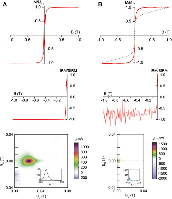
FIGURE 1. Hysteresis loop (top), back-field demagnetization (middle), and FORC distribution with an inset illustrating the coercivity spectrum (bottom) for (A) SD magnetosomes from M. gryphiswaldense (N.B., no correction for high-field slope is required); and (B) the SP synthetic magnetite (20 nm). Note dotted line shows hysteresis loop before correcting for high-field slope.

The hysteresis loop of the SP end member is closed and not saturated at 1 T (Figure 1B). The lack of saturation is due to poorly crystalline Fe phases that are in the colloid solution We correct this component for the high-field slope which will lead to an overcorrection for M_S. The overcorrection should not be large, because of the 20 nm particle size and a measurement averaging time of 100 ms. A weak IRM is detectable, but it is relaxing on the scale of the measurement as seen by the positive slope of the acquired remanence in high fields. The FORC distribution is centered at the origin of the diagram with a slight positive shift along the interaction axis (Figure 1B), as predicted by Pike et al. (2001).

SSD-SP Mixing Series

Because the SP end member does not carry a remanent magnetization, M_RS is used to monitor that the magnetic properties of the SSD end member is not changing with each addition of the SP end member. M_RS remains relatively constant until the SP contribution reaches 83% in the first mixing series, and its contribution dominates the overall magnetic properties, i.e., wasp-waisting of the loop becomes prominent. In the second series M_RS remains relatively constant for all increments, although there is no direct control over the amount of the SP material in the sample (Supplementary Figure S1).

The hysteresis loops for the samples in Series 1 illustrate that the magnetization is saturated by 300 mT (Supplementary Figure S2A). A gradual increase in wasp-waisting is seen, starting with 19% SP component that remains up to 91% (Supplementary Figure S3). For Series 2 only the magnetization of the SSD end member (sample one) and sample two are saturated by 300 mT (Supplementary Figure S2B); the other samples of the series show an approach to saturation. This will lead to an overcorrection for M_S, but the effect is on the order of a few percent (Kumari et al., 2015). Obvious wasp-waisting is not seen in Series 2, but there is a narrowing of the loop with each addition of the SP end-member (Supplementary Figure S4). The change in magnetic properties of both series can be compared by the change in M_RS/M_S and B_CR/B_C (Figure 2). There is a steady decrease in the magnetization ratio and increase in the coercivity ratio in both series. Series 1 plots left of Series 2 because of the larger size of the SP end member. The SP end member of Series 1, has a lower coercivity ratio than the second series, because the 20 nm core size allows for the measurement of B_CR from the magnetization that has not completely relaxed when the field is removed during the FORC measurement. Note that both series show lower coercivity ratios, i.e., lie to the left, of the theoretical curves from Dunlop (2002).

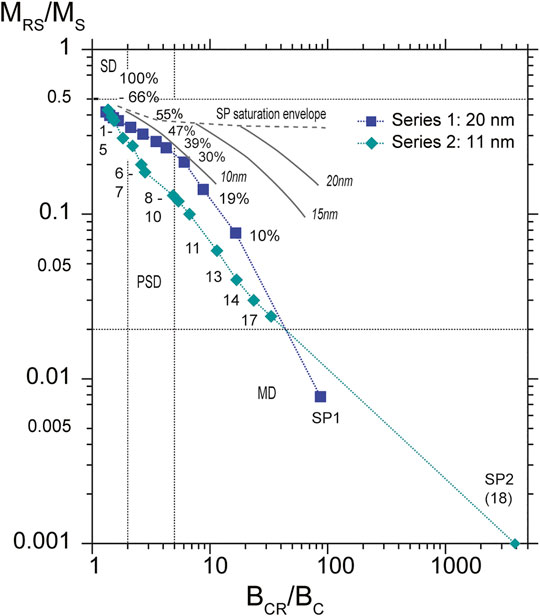
FIGURE 2. Day-Dunlop plot for both mixing series, in which the percentage refers to the total the SD end member in terms of total weight for the mixture Series 1. Note: we take the hysteresis parameters from the FORC measurements so that we compare Series 1 with Series 2 (cf. Supplementary Tables S1, S2). Gray lines show the SSD-SP mixing lines for 10, 15, and 20 nm particles taken from Dunlop (2002).

FORC diagrams show the gradual shift of the FORC distribution toward the origin with an increasing contribution of the SP component in Series 1 (Supplementary Figure S3). This is best seen in the coercivity profile with the growth of the peak at the origin. It is also reflected by an increase in the contribution of reversible component of the total magnetization at the expense of the irreversible contribution. Analysing the FORC data with PCA analysis using SF = 4, PC1 explains 85% of the variability, i.e., the relative concentration of the SSD and SP end members. The end members (EM) are clearly related to SSD (EM1) and SP (EM2) magnetite, and the PC1 score changes systematically with the relative change in the two end members (Figure 3A). The PCA approach reproduces the FORC diagram of SSD magnetite, but indicates a notable SP contribution, which is not as strongly expressed in the FORC diagrams (Supplementary Figure S3A). The FORC diagram for the SP end member also captures the main coercivity feature at the origin of the diagram, and shows the upward shift along the interaction field axis. The PCA analysis, however, also shows a very small SSD contribution (Supplementary Table S6). Using a higher smoothing factor leads to a narrower range in the PC1 score, which explains 92% of the variance. The PC1 score for the SP end member shifts closer to the sample with 91% SP-content (9% SSD concentration). The calculated FORC diagrams are similar to those described for SF = 4, but the SP contribution for EM1 and the SSD contribution to EM2 are more pronounced (Figure 3B; Supplementary Table S6).

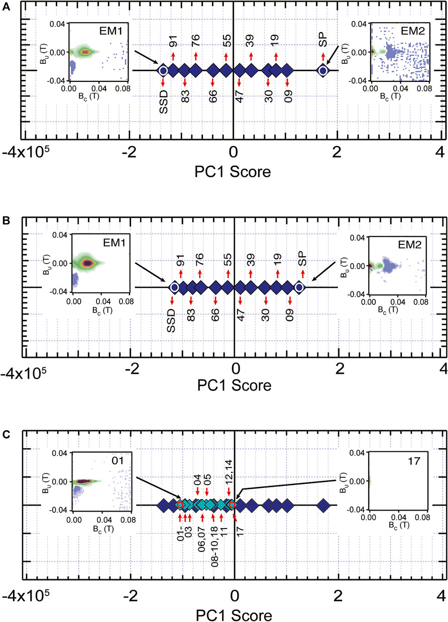
FIGURE 3. Binary PCA analysis from FORC data for (A) Series 1 with SF = 4; and (B) Series 1 with SF = 6 with FORC diagrams for end members (white circles) (C) Series 2 projected onto Series 1 with SF = 4; note that the FORC diagrams illustrate the predicted FORCs from the FORCem program for the extreme samples in the MK series (red circles). PCA grid is 1.54 mT in all PCA plots. Numbers refer to percentage of SP particles in (A) and (B), and sample number in (C).

Figure 3C shows the PC1 scores of the second series that are projected on the PC1 scores of the first series. There is a gradual shift in the PC1 score from the SSD end member to the SP end member of Series 2 (Figure 3C). The SSD end member has lies near an SSD contribution of ca. 86%, and the last SSD-SP sample, i.e., the sample with the highest SP component, lies close to the 50% SSD contribution of Series 1. The FORC diagram, which is calculated for the SSD end member, indicates a more prominent SP contribution than found in the measured FORC diagram (Supplementary Figure S4A). The PCA analysis, however, reproduces the FORC diagram for sample 17 (Supplementary Figure S4N). It is interesting that the SP end member of Series 2, shows a lower SP contribution than sample 17, which suggest that the PCA analysis cannot adequately resolve the contribution of these particles with faster relaxation time.

If we process the two sets of data together and use a PCA model that includes three end members, the third end member corresponds to a SSD assemblage, for the chains of magnetite. The second series shows a distinct separate progression in comparison to the first model (Supplementary Figures S5A,B). The calculated FORC diagram for the SSD end member of Series 2 (EM3) has a narrower distribution in interaction field (B_u), compared to Series 1. The calculated FORC for the SSD sample of Series 1, however, better resembles the measured FORC (cf., Supplementary Figures S3A, S5A).

The third method that we apply is to observe the change in M_rev/M_irrev as a function of B_C. If we assume that the SSD end member is made up of non-interacting, SSD magnetite and is controlled by shape anisotropy, then the irreversible contribution of magnetization should be 50% of the reversible contribution, and the ratio between the two would be 0.50 (Dunlop and Özdemir, 1997). For this reason the SP content should be reflected in the relative reversible contribution to magnetic hysteresis (Kumari et al., 2014). Figure 4 illustrates the change in ratio of the reversible to irreversible magnetization (M_rev/M_irrev). The coercivity of the SSD end member in Series 2 is lower than Series 1, which leads to a slight shift in the two curves. M_rev/M_irrev is <0.5 for the SSD end member of Series 1, which indicates that the sample does not meet the assumptions completely. This point is considered further in the discussion. As the contribution of M_rev to the total magnetization increases, B_C decreases as would be expected from what is observed in the Day-Dunlop plot.

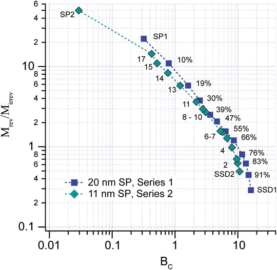
FIGURE 4. Change in M_rev/M_irrev as a function of B_C for Series 1 and 2 illustrating the progression from the SSD end members to SP end members. Percentages refer to SP% in Series 1 and numbers refer to sample number in Series 2.

Geological, Biological, and Material Samples

In order to investigate how applicable these methods may be in relation to natural or synthetic samples for which there is no information on the relative amounts of SP and SSD magnetite, we examine three sets of samples that have magnetite as the sole, or in some cases dominant, ferromagnetic phase. The first set include geological samples, the second are brain or brain tumour tissue from humans, and the third are synthesized magnetite. Samples from the three sets show narrow hysteresis loops that saturate in low fields (Supplementary Figures S6–S8). No obvious wasp-waisting was noted in any of the samples. The geological and biological samples show a range of magnetization and coercivity ratios when viewed on a Day-Dunlop plot (Figure 5). The lacustrine sediment and most of the brain tissue have open hysteresis loops, except for LH and SC, which have very narrow loops, and Tiva Canyon Tuff appears closed (Supplementary Figures S6, S7). Most of the geological and biological samples align close to Series 2. The synthetic samples show closed loops in the case of XL, AF23 and FCA35-250, but open loops for VR4, VR8, and FCA35-50 (Supplementary Figure S8). On the Day-Dunlop plot the synthetic samples show more deviation with respect to either series.

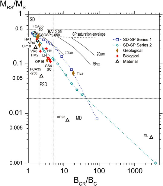
FIGURE 5. Day-Dunlop plot showing the change in the magnetization and coercivity ratios for the geological, biological and material samples in relation to the SD-SP series.

The lacustrine sediments for SOSP1-059, OP18, and BA10-05 have FORC diagrams that have elongated, narrow FORC distributions (Supplementary Figure S6), similar to the FORC diagrams of magnetotactic bacteria (cf., Supplementary Figures S3, S4). OP18, however also shows a secondary feature between ca. 20 and 30 mT with a broad distribution in B_U. This feature is common for magnetotactic bacteria in which magnetosomes cluster, due to disintegration of chains once the bacteria die (Kind et al., 2011). The FORC diagrams of the biological samples are characterized by distributions that lie close to the origin, with a SSD-like distribution for HA1 to more SP-like FORC distributions for SC, and LH (Supplementary Figure S7). Sample HA and GS have broader distributions in B_U compared to other samples. The Wohlfarth ratio for these samples is approximately 0.30 ± 0.05 (Brem et al., 2006), which indicates that there is interaction between the particles. In the material samples, the FORC diagrams for samples XL, AF23, and FCA35-250 show a confined distribution at the origin with an upward shift, indicative of the SP behaviour (Supplementary Figure S8). Samples VR4 and VR8 also have FORC distributions that are also close to the origin, but show a broader coercivity distribution. FCA35-50 has a FORC distribution that is away from the origin, indicating that the particles are magnetically blocked (Supplementary Figure S8).

PCA analysis was carried out on each set of samples and the PCA scores of each set projected onto the PCA scores of Series 1, which was processed with SF = 6. For the geological sample, the lacustrine samples, in which magnetite is bacterial, have a PC1 score are close to the sample with a 76–83% SSD concentration when projected on Series 1 (Figure 6A). Only the sample from the Tiva Canyon Tuff shows a higher contribution (ca. 50%) from the SP end member. The biological samples show PC1 scores that are similar to each other, lying between ca. 74 and 80% concentration of the SSD EM (Figure 6B). HA1 shows the strongest SSD contribution and LH the lowest, although differences between the samples is small (Figure 6B). The material set of samples shows more of a spread in PC1 scores, compared to the other two sample sets. XL lies beyond the SP end member of Series 1, and FCA35-50 lies nearest to the SSD end member (Figure 6C). The other samples are clustered between the Series 1 samples with 45–66% SSD content. A comparison of FCA35-250 and FCA35-50 illustrates a significant shift that occurs at lower temperature as the magnetic particles have undergone blocking.

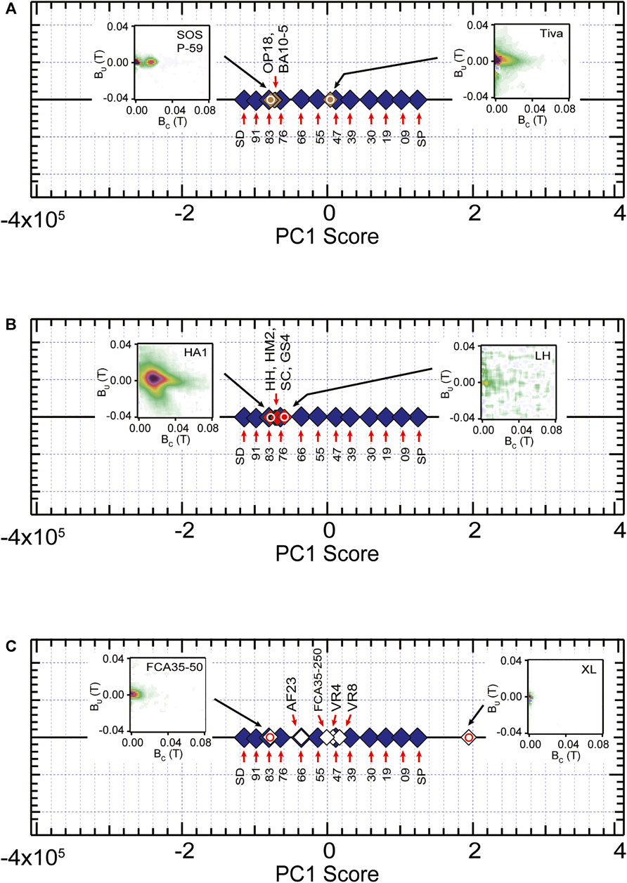
FIGURE 6. Binary PCA of FORC data for: (A) the geological samples (B) biological samples, and (C) material samples projected onto Series 1; FORC diagrams illustrate the predicted FORCs from the FORCem program for the extreme samples of each sample group (circles). The PCA grid is 1.54 mT and SF = 6 for all samples.

Plotting M_rev/M_irrev as a function B_C, shows that the geological set of samples follows the progression of Series 1 but is shifted toward higher B_C (Figure 7). The lacustrine samples cluster around the sample with 76% SSD concentration. The Tiva Canyon Tuff sample has a higher ratio that agrees with a higher concentration of SP magnetite. The biological samples lie close to Series 1 for the lowest values of M_rev/M_irrev, but then plot along the progression for the geological samples (Figure 7). M_rev/M_irrev falls below 0.5 for the two human brain samples that had Wohlfarth ratios around 0.3. Most of the material samples are also close to the progression found for Series 2, although with a shift to lower B_C. Only FCA35-50 is shifted to a higher coercivity.

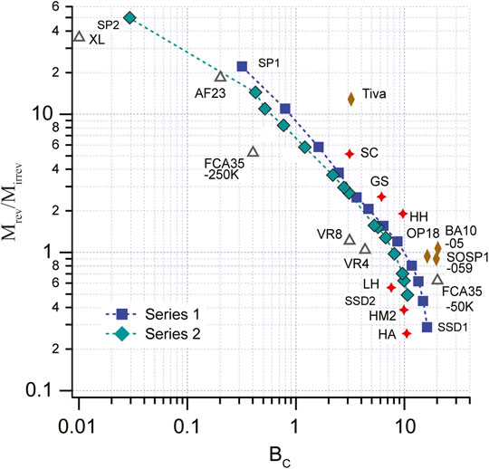
FIGURE 7. Change in M_rev/M_irrev as a function of B_C for the geological, biological and material samples in relation to Series 1 and 2.

Discussion

The two sets of SSD-SP mixtures show similarities in their change in magnetic properties that would be expected with an addition of a second phase that is ferromagnetic, but which carries “no” remanent magnetization. The difference between the two series arises largely from the difference in the core size of the SP end member, with 20 nm in Series 1 and ca. 11 nm in Series 2. Considering that the hysteresis and FORC measurements were made using an averaging time of 100 ms, this would mean that the boundary between SP and SSD behaviour for non-interacting magnetite is around 23 nm. Note the longest averaging time that was used in the FORC measurements was 300 ms, which would shift the boundary slightly higher to around 24 nm.

The two SP end members do not show any frequency dependency with respect to the applied frequencies; therefore, χ_FD cannot be used to provide information on the concentration of SP particles. Our results highlight the limitations of using the methods due to the frequencies that are available in commercial instruments.

The hysteresis loops for Series 1 show wasp-waisting with the addition of the SP end member starting between 9 and 19% SP-content. Series 2, however, only shows a weak wasp-waisting by sample 10; what is notable, however, is a narrowing of the hysteresis loop. This difference reflects probably the more rapid relaxation of particles in Series 2. The Day-Dunlop plot is one of the most commonly employed methods to assess particle size or domain state of magnetite, based on hysteresis parameters. There is a major concern, which is associated with using hysteresis properties, to estimate particles size. Day et al. (1977) noted that if magnetite particles are interacting, this will lower M_RS/M_S, B_C and B_CR. Muxworthy et al. (2003) examined the effect of magnetostatic interactions of hysteresis parameters using micromagnetic models, and demonstrated that the degree to which the parameters will be affected, will be dependent on particle anisotropies, degree of alignment, and particle configuration. For magnetite in the SSD range, magnetostatic interactions can lead to significantly lower values of M_RS/M_S, B_C and B_CR.

Dunlop (2002) presented a theoretical study in which he demonstrated how hysteresis parameters will change for SSD-SP mixtures, for SP particles between 10 and 30 nm. Dunlop and Carter-Stiglitz (2006) carried out an experimental study on the hysteresis properties of a mixture of SSD magnetite and a ferrofluid of SP magnetite, and found that B_CR/B_C was lower than predicted, which they attributed to interactions. Roberts et al. (2018), provides a thorough discussion of the weakness of using this method, where they note, among other points, that Dunlop (2002) does not consider thermal relaxation in his mixtures of SSD-SP magnetite, which will have an effect on the magnetization ratio. When thermal relaxation of the viscous particle is considered, there is a more rapid drop in M_RS/M_S (Lanci and Kent, 2003; Kumari et al., 2015; Roberts et al., 2018). This is supported by experimental results (Dunlop-Cater-Stiglitz, 2006; Kumari et al., 2015).

Figure 2 shows the progression of M_RS/M_S and B_CR/B_C for the two SSD-SP series. Series 1 has higher coercivity ratios relative to Series 2, which would be expected due to the larger volume of the SP particles. How this is reflected in the natural samples or synthetic magnetic nanoparticles is seen in Figure 5. The samples from the three sets, which show coercivity ratios that would require the presence of very fine particles (<10 nm), according to Dunlop’s (2002) theoretical results. The coercivity ratios, however, are consistent for a broad particle size spectra in the SP range when accounting for thermal relaxation (Lanci and Kent, 2003). It should also be noted that none of these three sets of samples show wasp-waisting (Supplementary Figures S6–S8). Samples AF23 and XL are synthetic nanoparticles with better constrained particle sizes that are close to the SP-SSD boundary. These two samples show the lowest magnetization ratios, similar to what was found in the SP end member of the mixing series. In summary there is a progression to lower values of M_RS/M_S and higher values of B_CR/B_C with increasing SP concentration, but all sample sets lie below the theoretical progression that is expected by only assuming Langevin behaviour.

The FORC diagrams for Series 1 shows a gradual progression of a FORC distribution from a diagram typical for SSD magnetite, which lies away from the origin. The first indication of an SP contribution at the origin of the FORC diagram is for the sample with 19% SP content, and this contribution becomes larger successively with each addition (Supplementary Figure S3). The SP end-member is confined to the origin with a slight upward shift. The second series only has a FORC distribution that is typical for magnetotactic bacteria with a broader coercivity spectrum that extends to the origin of the plot. There is no noticeable change in the FORC diagram, other than a gradual decrease in the intensity of the distribution, until the until 10th addition, when the hysteresis loop shows a weak wasp-waisting. The SP end member has only a weak expression at the origin, which suggests that the FORCs will be less influenced due to the faster relaxation of the smaller particle diameter in comparison to the SP end member of Series 1.

PCA analysis of the FORC data provides a more quantitative way to observe changes. Series 1 shows a regular change in the PC1 score with each increment (Figure 3; Supplementary Table S6), and the calculated FORC diagrams of the end members are in agreement with the FORC diagrams in their major features. If we compare Series 2 with Series 1, the starting SSD end member has a notable SP-contribution (86% SSD-concentration). The sample with the highest SP concentration (sample 17) compares with the sample with ca. 50% SSD--concentration, but the SP end-member of Series 2 falls around the 68% concentration of Series 1. The fact that a higher SSD concentration is predicted for the SP end member of Series 2 indicates that the PCA cannot properly assess the SP end member with its fast relaxation. This point is discussed below.

A comparison of the samples from geological samples projected onto Series 1 shows that the lacustrine sediments fall toward an SSD concentration of around 76–83% of Series 1 in PCA analysis (Figure 6). Bacterial magnetite is thought to be the main source of magnetite in the samples and this comparable to the SD end member of Series 2, which is bacterial magnetite. The Tiva Canyon Tuff sample lies by ca. 50% contribution of SP particles from Series 1 similar to the higher SP concentration in Series 2. Note that a largely SP content that was found by Till et al. (2011) from low temperature blocking in field-cooled and zero-field-cooled experiments. The biological samples also lie around an SSD concentration of around 74–80%. Note that all of the biological samples show an increase in isothermal remanent magnetization when measured at 77 K (Brem, 2006; Blaser, 2008). This confirms that all samples contain a certain amount of SP magnetite, but it is not possible to determine the concentration. The synthetic samples show a larger spread in particle size, which is in agreement to physical measurements. Samples VR4 and VR8 are mesocrystals of magnetite made up of ca. 9–11 nm crystallites that agglomerate into a single crystal with 45 nm diameter. The SP content reflects the remainder of crystallites or smaller aggregates in the colloidal solution (Reichel et al., 2017). Sample FCA35 is a synthetic magnetite with ca. 16 ± 1 nm core (pers. comm. F. Crippa). It is SP at room temperature but undergoes partial blocking at 250 K, where the PCA analysis suggest that ca. 50% of the magnetization is blocked. At 50 K, ca. 83% of the magnetization is blocked in comparison to Series 1. AF23 has a 23 ± 1 nm magnetite core (pers. comm. A. Fink), which is close to the SP-SSD boundary, and the same is found for XL, whose core diameter is close to being magnetically ordered at room temperature (Hirt et al., 2017). The two samples, however, have markedly different PC1 scores. Although it is difficult to reconcile this difference, it should be noted that AF23 consists of a single magnetite crystal, whereas XL is a mesocrystal, i.e., an assemblage of smaller subunits, in which all have the same crystallographic orientation.

The last method to qualitatively assess the SP contribution to the magnetization is a comparison of the reversible to irreversible magnetization. This method assumes that magnetite is non-interacting as in the case of the Day-Dunlop plot. Both mixing series show an increase in M_rev/M_irrev with increasing SP concentration. This parameter can be plotted as a function of B_C, which will decrease as the SP-content increases. We use a log plot, because the increase in the ratio is small for low concentrations for the SP end member. There is a progressive increase in M_rev/M_irrev accompanied by the decrease in B_C, which would be expected. The track that the progression follows will be sensitive to the coercivity of the SSD end member, i.e., where the progression starts on the plot. This effect is seen for the lake sediments that have a higher coercivity than the SSD end member of Series 1, and therefore lie to the higher coercivity end of Series 1. The size of the SP end member affects how rapidly M_rev/M_irrev will increase; therefore, higher M_rev/M_irrev will be reached for lower SP content. Although one would expect M_rev/M_irrev < 0.5 for magnetite that is controlled by magnetocrystalline anisotropy, it is also found in the samples for which there is independent evidence for interaction between particles (Wohlfarth ratios).

Plots of ∂M_rev/∂B and ∂M_irrev/∂B are also of value (cf., Supplementary Figures S3, S4, S6–S8). For Series 1 M_irrev is characterized by a Gaussian curve. With the first addition of an SP component, little change is seen in the general shape of the hysteresis curve, or the FORC diagram, but the Gaussian curve shows a weak deviation on its flank around ∂B = 0. This feature becomes stronger with each addition of the SP material until two separate peaks are seen. It is these two distinct coercivity contributions that lead to wasp-waisting in the hysteresis curve. Note, in the case of Series 2, however, this secondary peak is not seen in M_irrev.

In summary, three methods were evaluated for detecting SP magnetite in mixtures with SSD magnetite. Both the Day-Dunlop plot and M_rev/M_irrev will see a progression that is related to the amount of SP particles in a material. Critical for the progression in the Day-Dunlop plot is the SP particles size, whereas it is the coercivity of the SSD end member that will be important for M_rev/M_irrev plotted as a function of B_C. Both methods, however, assume that the magnetite is non-interacting. If interactions occur between the magnetite particles, then there will be a reduction in M_RS/M_S, B_C, and B_CR, which would predict falsely a higher SP concentration. This may not be serious for weak interactions, as seen in the example of OP 18 compared to SOSP1-059, but would not be suitable for an assembly of interacting particles. A critical point is that both approaches are also not applicable if there are particles that are larger than SSD, which would also contribute to the reversible magnetization.

FORC analysis and PCA of the FORC measurements is suitable in detecting SP content, particularly when the SP particles are near to the SP-SSD boundary. The method loses its sensitivity when the SP particles are very fine and have short relaxation times. Fine SP particles will still contribute to the induced magnetization, which is why they affect hysteresis and M_rev/M_irrev, but will have less of a contribution to the FORC distribution. The SP concentration, which the PCA analysis calculates, will be dependent on knowing what the correct end members are so that they can be fitted. This can often be a limiting factor, particularly in natural samples that can show variability within a given locality, and the number of end members may not be clear. The smoothing factor, which is used to process the FORCs, will also play a role in any comparison of FORC results, therefore all data sets should be processed using the same smoothing factor.

In addition to problems that will arise if there are particles that are larger than SSD, or are interacting magnetically, we extend further caveats with respect to all three approaches. Firstly, the presence of other mineral phases, e.g., hematite, will greatly affect hysteresis properties. Mixtures of different ferromagnetic minerals with different particle sizes will lead to competing factors, which will not be possible to separate. Secondly, performing a slope correction could remove part of the contribution from the superparamagnetic contribution. Thirdly, averaging time of measurements is another factor that needs consideration and plays an important role in any comparison. Samples should only be evaluated if their measurement has been made using the same averaging time. Longer averaging time will lead to more relaxation during a measurement, thus influencing the reversible magnetization.

We can ask how often one deals with ideal mixtures of SSD-SP particles that are only made up of non-interacting magnetite. They are most likely to be found in synthetic particles, and the above approaches can be very useful in the characterization of these systems. Depending on the source of the ferromagnetic particles in biological systems, these are also often limited to finer particles. The problem in tissue samples, however can be clustering, and therefore meeting the criterion of non-interaction. For example, Brem et al. (2006) found clustering between magnetite/maghaemite particles in the brain tissues that were studied, but measurements had to be made on freeze-dried tissue that was compressed. They could not conclude if the particles were clustered naturally or due to sample preparation. In any case these presented methods can provide useful information in a comparison of different tissues, although some overestimation of the SP concentration may occur. The same can be said for natural materials. These can have more variety in the composition of ferromagnetic (s.l.) phases, and in particle size, which may not include only SP and SSD particle size. The degree of magnetic interaction may also be more common. Critical is that magnetite is the main ferromagnetic phase, and there is independent evidence that the effect due to interactions is not large.

Conclusion

We have evaluated three methods to estimate the relative contribution of SP magnetite to mixtures with SSD magnetite, using two mixing series of SSD magnetite with SP magnetite, which have two different particle sizes. Both the Day-Dunlop plot or M_rev/M_irrev plotted as a function of B_C will detect changes in the SP contribution to the magnetization. PCA analysis of FORC measurements will also detect changes in the relative amount of SP particles, but is less sensitive in distinguishing small differences. The particle size or size distribution will affect the relatively change in magnetization with increasing SP concentration in all three methods. For this reason, the methods provide a qualitative method for assessing the concentration of SP magnetite, although comparisons within a selected group of samples may provide semi-quantitative information.

Data Availability Statement

The raw data supporting the conclusions of this article will be made available by the authors, without undue reservation.

Ethics Statement

The studies involving human participants were reviewed and approved by University Hospital- Zurich Medical Ethics Committee. Written informed consent for participation was not required for this study in accordance with the national legislation and the institutional requirements.

Author Contributions

PL and AH contributed equally to the experimental design, data acquisition, data evaluation and writing the manuscript.

Funding

PL acknowledges support from the financial support from the following agencies: China Scholarship Council (No. 201706410009), the Science and Technology Development Fund, Macau SAR (Project No. 0002/2019/APD).

Conflict of Interest

The authors declare that the research was conducted in the absence of any commercial or financial relationships that could be construed as a potential conflict of interest.

Acknowledgments

We thank M. Kumari for her helpful discussion. A. Petro-Fink and F. Crippa are acknowledged for use of their magnetic nanoparticle samples, and O. Paasche for sample OP18. We gratefully acknowledged the comments of two reviewers and L. Sagnotti for improving this manuscript.

Supplementary Material

The Supplementary Material for this article can be found online at: https://www.frontiersin.org/articles/10.3389/feart.2020.586913/full#supplementary-material.

References

Beyhum, W., Hautot, D., Dobson, J., and Pankhurst, Q. A. (2005). Magnetic biomineralisation in huntington’s disease transgenic mice. J. Phys. Conf. Ser. 17, 50–53. doi:10.1088/1742-6596/17/1/008
Blaser, C. (2008). Magnetic iron mineralogy in human tissue from brain tumors. Zürich, Switzerland: University of Zürich.
Brem, F., Hirt, A. M., Winklhofer, M., Frei, K., Yonekawa, Y., Wieser, H. G., et al. (2006). Magnetic iron compounds in the human brain: a comparison of tumour and hippocampal tissue. J. R. Soc. Interface. 3, 833–841. doi:10.1098/rsif.2006.0133
Brem, F. K. (2006). Magnetic characterization of iron phases in human brain tissue: application to epileptic and tumour tissue. Zürich, Switzerland: ETH Zürich.
Calderon-Garciduenas, L., Gonzalez-Maciel, A., Mukherjee, P. S., Reynoso-Robles, R., Perez-Guille, B., Gayosso-Chavez, C., et al. (2019). Combustion and friction-derived magnetic air pollution nanoparticles in human hearts. Environ. Res. 176, 108567. doi:10.1016/j.envres.2019.108567
Crippa, F., Moore, T. L., Mortato, M., Geers, C., Haeni, L., Hirt, A. M., et al. (2017). Dynamic and biocompatible thermo-responsive magnetic hydrogels that respond to an alternating magnetic field. J. Magn. Magn Mater. 427, 212–219. doi:10.1016/j.jmmm.2016.11.023
Crippa, F., Rodriguez-Lorenzo, L., Hua, X., Goris, B., Bals, S., Garitaonandia, J. S., et al. (2019). Phase transformation of superparamagnetic iron oxide nanoparticles via thermal annealing: implications for hyperthermia applications. ACS Appl. Nano Mater. 2, 4462–4470. doi:10.1021/acsanm.9b00823
Day, R., Fuller, M., and Schmidt, V. A. (1977). Hysteresis properties of titanomagnetite: grain size and compositional dependence. Phys. Earth Planet. Inter. 13, 260–267. doi:10.1016/0031-9201(77)90108-X
Dearing, J. R., Dann, R. J. L., Hay, K., Lees, J. A., Loveland, P. J., Maher, B. A., et al. (1996). Frequency-dependent susceptibility measurements of environmental materials. Geophys. J. Int. 124, 228–240. doi:10.1111/j.1365-246X.1996.tb06366.x
Dekkers, M. J. (1988). Some rock magnetic parameters for natural goethite, pyrrhotite, and fine-grained hematite. PhD dissertation. Utrecht (Netherlands): University of Utrecht.
Dobson, J. (2004). Magnetic iron compounds in neurological disorders. Ann. N. Y. Acad. Sci. 1012, 183–192. doi:10.1196/annals.1306.016
Dunlop, D. J. (2002). Theory and application of the Day plot (Mrs/Ms versus Hcr/Hc) 1. Theoretical curves and tests using titanomagnetite data. J. Geophys. Res. Solid Earth. 107, 2056. doi:10.1029/2001jb000486
Dunlop, D. J., and Carter-Stiglitz, B. (2006). Day plots of mixtures of superparamagnetic, single-domain, pseudosingle-domain, and multidomain magnetites. J. Geophys. Res. Solid Earth. 111, B12S09. doi:10.1029/2006JB004499
Dunlop, D. J., and Özdemir, Ö. (1997). Rock magnetism: fundamentals and Frontiers. Cambridge, United Kingdom: Cambridge University Press.
Egli, R. (2004a). Characterization of individual rock magnetic components by analysis of remanence curves. 2. Fundamental properties of coercivity distributions. Phys. Chem. Earth. 29, 851–867. doi:10.1016/j.pce.2004.04.001
Egli, R. (2004b). Characterization of individual rock magnetic components by analysis of remanence curves. 3. Bacterial magnetite and natural processes in lakes. Phys. Earth Planet. Int. 29, 869–884. doi:10.1016/j.pce.2004.03.010
Egli, R. (2003). Environmental influences on the magnetic proeprties of lake sediments. Zürich, Switzerland: ETH-Zurich.
Egli, R. (2013). VARIFORC: an optimized protocol for calculating non-regular first-order reversal curve (FORC) diagrams. Global Planet. Change. 110, 302–320. doi:10.1016/j.gloplacha.2013.08.003
Faivre, D., and Schüler, D. (2008). Magnetotactic bacteria and magnetosomes. Chem. Rev. 108, 4875–4898. doi:10.1021/cr078258w
Geiss, C. E., Heider, F., and Soffel, H. C. (1996). Magnetic domain observations on magnetite and titanomaghemite grains (0.5-10mm). Geophys. J. Int. 124, 75–88. doi:10.1111/j.1365-246X.1996.tb06353.x
Harrison, R. J., and Feinberg, J. M. (2008). FORCinel: an improved algorithm for calculating first‐order reversal curve distributions using locally weighted regression smoothing. Geochem. Geophys. Geosyst. 9, Q05016. doi:10.1029/2008GC001987
Harrison, R. J., Muraszko, J., Heslop, D., Lascu, I., Muxworthy, A. R., and Roberts, A. P. (2018). An improved algorithm for unmixing first‐order reversal curve diagrams using principal component analysis. Geochem. Geophys. Geosyst. 19, 1595–1610. doi:10.1029/2018GC007511
Heider, F. (1988). Magnetic properties of hydrothermally grown Fe3O4 crystals. PhD dissertation, Toronto (ON): University of Toronto.
Heider, F., Zitzelsberger, A., and Fabian, F. (1996). Magnetic susceptibility and remanent coercive force in grown magnetite crystals from 0.1 µm to 6 mm. Phys. Earth Planet. Int. 93, 239–256. doi:10.1016/0031-9201(95)03071-9
Heslop, D. (2005). A Monte Carlo investigation of the representation of thermally activated single-domain particles within the day plot. Stud. Geophys. Geod. 49, 163–176. doi:10.1007/s11200-005-0003-7
Hirt, A. M., Kumari, M., Heinke, D., and Kraupner, A. (2017). Enhanced methods to estimate the efficiency of magnetic nanoparticles in imaging. Molecules 22, 2204. doi:10.1039/c6ra03115c
Hosking, D. E., Ayton, S., Beckett, N., Booth, A., and Peters, R. (2018). More evidence is needed. Iron, incident cognitive decline and dementia: a systematic review. Ther. Adv. Chron. Dis. 9, 241–256. doi:10.1177/2040622318788485
Hrouda, F. (2011). Models of frequency-dependent susceptibility of rocks and soils revisited and broadened. Geophys. J. Int. 187, 1259–1269. doi:10.1111/j.1365-246X.2011.05227.x
Ilyashuk, E. A., Koinig, K. A., Heiri, O., Ilyashuk, B. P., and Psenner, R. (2011). Holocene temperature variations at a high-altitude site in the Eastern Alps: a chironomid record from Schwarzsee ob Sölden, Austria. Quat. Sci. Rev. 30, 176–191. doi:10.1016/j.quascirev.2010.10.008
Jacob, J. J., and Suthindhiran, K. (2016). Magnetotactic bacteria and magnetosomes—scope and challenges. Mater. Sci. Eng. C Mater. Biol. Appl. 68, 919–928. doi:10.1016/j.msec.2016.07.049
Katzmann, E., Eibauer, M., Lin, W., Pan, Y., Plitzko, J. M., and Schüler, D. (2013). Analysis of magnetosome chains in magnetotactic bacteria by magnetic measurements and automated image analysis of electron micrographs. Appl. Environ. Microbiol. 79, 7755–7762. doi:10.1128/AEM.02143-13
Kind, J., Gehring, A. U., Winklhofer, M., and Hirt, A. M. (2011). Combined use of magnetometry and spectroscopy for identifying magnetofossils in sediments. Geochem. Geophys. Geosyst. 12, Q08008. doi:10.1029/2011GC003633
Kumari, M., Hirt, A. M., Uebe, R., Schuler, D., Tompa, É., Posfai, M., et al. (2015). Experimental mixtures of superparamagnetic and single-domain magnetite with respect to Day-Dunlop plots. Geochem. Geophys. Geosyst. 16, 1739–1752. doi:10.1002/2015GC005744
Kumari, M., Widdrat, M., Tompa, E., Uebe, R., Schuler, D., Mihaly, P., et al. (2014). Distinguishing magnetic particle size of iron oxide nanoparticles with first-order reversal curves. J. Appl. Phys. 116, 124304. doi:10.1063/1.4896481
Lanci, L., and Kent, D. V. (2003). Introduction of thermal activation in forward modeling of hysteresis loops for single-domain magnetic particles and implications for the interpretation of the Day diagram. J. Geophys. Res. Solid Earth. 108, 2124. doi:10.1029/2001jb000944
Lascu, I., Harrison, R. J., Li, Y., Muraszko, J. R., Channell, J. E. T., Piotrowski, A. M., et al. (2015). Magnetic unmixing of first‐order reversal curve diagrams using principal component analysis. Geochem. Geophys. Geosyst. 16, 2900–2915. doi:10.1002/2015GC005909
Liu, P. F., Hirt, A. M., Schuler, D., Uebe, R., Zhu, P. M., Liu, T. Y., et al. (2019). Numerical unmixing of weakly and strongly magnetic minerals: examples with synthetic mixtures of magnetite and hematite. Geophys. J. Int. 217, 280–287. doi:10.1093/gji/ggz022
Lohsse, A., Kolinko, I., Raschdorf, O., Uebe, R., Borg, S., Brachmann, A., et al. (2016). Overproduction of magnetosomes by genomic amplification of biosynthesis-related gene clusters in a magnetotactic bacterium. Appl. Environ. Microbiol. 82, 3032–3041. doi:10.1128/AEM.03860-15
Maher, B. A., Ahmed, I. A., Karloukovski, V., Maclaren, D. A., Foulds, P. G., Allsop, D., et al. (2016). Magnetite pollution nanoparticles in the human brain. Proc. Natl. Acad. Sci. U.S.A. 113, 10797–10801. doi:10.1073/pnas.1605941113
Moskowitz, B. M., Frankel, R., and Bazylinski, D. (1993). Rock magnetic criteria for the detection of biogenic magnetite. Earth Planet. Sci. Lett. 120, 283–300. doi:10.1016/0012-821X(93)90245-5
Muxworthy, A., Williams, W., and Virdee, D. (2003). Effect of magnetostatic interactions on the hysteresis parameters of single-domain and pseudo-single-domain grains. J. Geophys. Res. Solid Earth. 108, 2517. doi:10.1029/2003jb002588
Newell, A. J. (2005). A high-precsion model of first-order reversal curve (FORC) functions for single-domain ferromagnetic with uniaxial anisotropy. Geochem. Geophsy. Geosys. 6, Q05010. doi:10.1029/2004GC00877
Pike, C. R., Roberts, A. P., and Verosub, K. L. (2001). First-order reversal curve diagrams and thermal relaxation effects in magnetic particles. Geophys. J. Int. 145, 721–730. doi:10.1046/j.0956-540x.2001.01419.x
Reichel, V., Kovács, A., Kumari, M., Bereczk-Tompa, É., Schneck, E., Diehle, P., et al. (2017). Single crystalline superstructured stable single domain magnetite nanoparticles. Sci. Rep. 7, 45484. doi:10.1038/srep45484
Roberts, A. P., Tauxe, L., Heslop, D., Zhao, X., and Jiang, Z. X. (2018). A critical appraisal of the "Day" diagram. J. Geophys. Res. Solid Earth. 123, 2618–2644. doi:10.1002/2017JB015247
Sotiriou, G. A., Hirt, A. M., Lozach, P. Y., Teleki, A., Krumeich, F., and Pratsinis, S. E. (2011). Hybrid, silica-coated, janus-like plasmonic-magnetic nanoparticles. Chem. Mater. 23, 1985–1992. doi:10.1021/cm200399t
Starsich, F. H., Sotiriou, G. A., Wurnig, M. C., Eberhardt, C., Hirt, A. M., Boss, A., et al. (2016). Silica-coated nonstoichiometric nano Zn-ferrites for magnetic resonance imaging and hyperthermia treatment. Adv. Healthcare Mater. 5, 2698–2706. doi:10.1002/adhm.201600725
Starsich, F. H. L., Eberhardt, C., Boss, A., Hirt, A. M., and Pratsinis, S. E. (2018). Coercivity determines magnetic particle heating. Adv. Healthcare Mater. 7, e1800287. doi:10.1002/adhm.201800287
Storen, E. W. N., Paasche, O., Hirt, A. M., and Kumari, M. (2016). Magnetic and geochemical signatures of flood layers in a lake system. Geochem. Geophys. Geosyst. 17, 4236–4253. 10.1002/2016GC006540
Sweetkind, D. S., Reynolds, R. L., Sawyer, D. A., and Rosenbaum, J. G. (1993). Effects of hydrothermal alteration on the magnetization of the oligocene carpenter ridge tuff, bachelor caldera, san juan mountains, Colorado. J. Geophys. Res.: Solid Earth. 98, 6255–6266. doi:10.1029/93JB00014
Tauxe, L., Mullender, T. A. T., and Pick, T. (1996). Potbellies, wasp-waists, and superparamagnetism in magnetic hysteresis. J. Geophys. Res. Solid Earth. 101, 571–583. doi:10.1029/95JB03041
Till, J. L., Jackson, M. J., Rosenbaum, J. G., and Solheid, P. (2011). Magnetic properties in an ash flow tuff with continuous grain size variation: a natural reference for magnetic particle granulometry. Geochem. Geophsy. Geosyst. 12, Q07Z26. doi:10.1029/2011GC003648
Widdrat, M., Kumari, M., Tompa, É., Pósfai, M., Hirt, A. M., and Faivre, D. (2014). Keeping nanoparticles fully functional: long-term storage and alteration of magnetite. Chempluschem. 79, 1225–1233. doi:10.1002/cplu.201402032
Keywords: magnetite, superparamagnetic-single domain mixtures, Day-Dunlop plot, FORC- PCA analysis, reversible-irreversible magnetization
Citation: Hirt AM and Liu P (2021) Estimating the Relative Concentration of Superparamagnetic and Stable Single Domain Particles in Geological, Biological, and Synthetic Materials. Front. Earth Sci. 8:586913. doi: 10.3389/feart.2020.586913
Received: 24 July 2020; Accepted: 24 December 2020;
Published: 16 February 2021.
Edited by:
Leonardo Sagnotti, Istituto Nazionale di Geofisica e Vulcanologia (INGV), ItalyReviewed by:
David Heslop, Australian National University, AustraliaRamom Egli, Central Institution for Meteorology and Geodynamics (ZAMG), Austria
Copyright © 2021 Hirt and Liu. This is an open-access article distributed under the terms of the Creative Commons Attribution License (CC BY). The use, distribution or reproduction in other forums is permitted, provided the original author(s) and the copyright owner(s) are credited and that the original publication in this journal is cited, in accordance with accepted academic practice. No use, distribution or reproduction is permitted which does not comply with these terms.
*Correspondence: Ann M. Hirt, ann.hirt@erdw.ethz.ch