Hexagonal fuzzy approximation of fuzzy numbers and its applications in MCDM

Abstract

Numerous research papers and several engineering applications have proved that the fuzzy set theory is an intelligent effective tool to represent complex uncertain information. In fuzzy multi-criteria decision-making (fuzzy MCDM) methods, intelligent information system and fuzzy control-theoretic models, complex qualitative information are extracted from expert’s knowledge as linguistic variables and are modeled by linear/non-linear fuzzy numbers. In numerical computations and experiments, the information/data are fitted by nonlinear functions for better accuracy which may be little hard for further processing to apply in real-life problems. Hence, the study of non-linear fuzzy numbers through triangular and trapezoidal fuzzy numbers is very natural and various researchers have attempted to transform non-linear fuzzy numbers into piecewise linear functions of interval/triangular/trapezoidal in nature by different methods in the past years. But it is noted that the triangular/trapezoidal approximation of nonlinear fuzzy numbers has more loss of information. Therefore, there is a natural need for a better piecewise linear approximation of a given nonlinear fuzzy number without losing much information for better intelligent information modeling. On coincidence, a new notion of Generalized Hexagonal Fuzzy Number has been introduced and its applications on Multi-Criteria Decision-Making problem (MCDM) and Generalized Hexagonal Fully Fuzzy Linear System (GHXFFLS) of equations have been studied by Lakshmana et al. in 2020. Therefore, in this paper, approximation of nonlinear fuzzy numbers into the hexagonal fuzzy numbers which includes trapezoidal, triangular and interval fuzzy numbers as special cases of Hexagonal fuzzy numbers with less loss/gain of information than other existing methods is attempted. Since any fuzzy information is satisfied fully by its modal value/core of that concept, any approximation of that concept is expected to be preserved with same modal value/core. Therefore, in this paper, a stepwise procedure for approximating a non-linear fuzzy number into a new Hexagonal Fuzzy Number that preserves the core of the given fuzzy number is proposed using constrained nonlinear programming model and is illustrated numerically by considering a parabolic fuzzy number. Furthermore, the proposed method is compared for its efficiency on accuracy in terms of loss of information. Finally, some properties of the new hexagonal fuzzy approximation are studied and the applicability of the proposed method is illustrated through the Group MCDM problem using an index matrix (IM).

Introduction

Most of the real-life problems are involved with complex forms of uncertain information which are continuous transitions. Zadeh introduced a fuzzy set (FS) in 1965 to deal with such information which has a wide scope of applications in many research fields such as expert systems, pattern recognition, data mining. In this queue, defuzzification methods have been widely developed and are implemented in several research areas like MCDM, fuzzy control, data analysis, and clustering, etc. The approximation is a better kind of defuzzification with a reliable agreement balancing appropriate form of approximation to enhance better computation and preventing loss of information as much as possible. In the past years, various researchers have investigated approximation of general non-linear fuzzy numbers by linear fuzzy numbers of simpler forms such as interval, triangular and trapezoidal to avoid complex calculations in the problems involving nonlinear fuzzy numbers. All these reasons cause a natural need for a better approximation of fuzzy numbers that are easy to handle without losing much information. In this section, a detailed literature review and motivation are given as subsections.

Literature review

The interval approximation of fuzzy numbers (FNs) is initially started using Hamming distance on intervals by Stephen chanas [23] and later is developed using Euclidean metric on intervals based on the $\alpha$-cuts by Grzegorzewski [33]. Later, it is extended to another simpler form of triangular approximation with symmetricity and non-symmetricity by Ma et al. [47] and Zeng and Li [68]. In that sequel, Abbasbandy and Asady [3] have proposed a new technique to defuzzify a fuzzy quantity by trapezoidal fuzzy numbers (TPFNs). In 2005, Grzegorzewski and Mrowka [36] propounded trapezoidal approximation using the metric by preserving the expected interval, and later, it was proved that the method does not lead always a FN. Hence they [37] revisited the trapezoidal approximation operator by preserving the expected interval (EI). Abbasbandy and Amirfakhrian [1] have recommended an ideal method to enumerate the proximate approximation of a fuzzy number as a polynomial. They [2] also suggested a nearest trapezoidal form of a FN using pseudo metric on the set of all FNs by considering generalized LR type fuzzy number. In 2007, Zeng and Li [68] put forth the approximation procedure by a triangular fuzzy number (TRFN) followed by the approach of Grzegorzewski’s trapezoidal approximation technique defined in [36].

To overcome the flaws that occurred in [36, 37, 68], Ban [8, 9] redefined the approximation methods in 2008 using Karush Kuhn Tucker (KKT) Theorem by upholding the expected interval, value, ambiguity, width, and weighted expected value. Continuing with that, Grzegorzewski [34] has expressed the algorithms and properties for computing the proper trapezoidal approximation for a fuzzy number by preserving the expected interval. Moreover in 2008, Yeh [63] has investigated the Zeng and Li approximation and he improved it by extended triangular and trapezoidal approximation. He [64] improved Grzegorzewski’s approximation operator defined in [34] and proposed a procedure for calculating the improved approximation. Ban [10] has proposed the parametric approximation using the average Euclidean distance of a given FN. He [11] also suggested the triangular and parametric approximations of FNs by correcting the inadvertences of Zeng and Li’s [68] and Gregorzewski’s [36] nearest parametric approximation using the KKT theorem. In 2010, Grzegorzewski [35] has recommended a new approach for finding trapezoidal approximation preserving the expected interval. Ban [4, 19] put forward a new approximation method of trapezoidal type FN by perpetuating core, expected value, ambiguity, value, and discussed some of its properties. Ban [12] has discussed the significance of translation invariance and scale invariance in approximation techniques. He [13] also expressed the metric properties of the nearest extended parametric FN which generalizes the extended trapezoidal fuzzy number and parametric fuzzy number. Ban [14, 15] has proposed the nearest interval, triangular, trapezoidal, and weighted semi trapezoidal approximation of FN preserving ambiguity and weighted ambiguity in 2012.

Coroianu [24] has introduced some properties of convex subsets of topological spaces with Euclidean distance in the field of fuzzy numbers. It is a very useful tool to compute the Lipschitz constant of the trapezoidal operator preserving the value and ambiguity. In 2014, Ban [16] has recommended the conditions for existence, uniqueness, and continuity of the trapezoidal approximation of the FN. Coroianu [28] has considered different parameters named max product Bernstein operators for the approximation of FNs. In 2014, Gregorzewski [38] has suggested a new trapezoidal operator preserving core, support, and expected interval which guarantees the proper interpretation of the solution even for skew fuzzy numbers. Yeh in 2014, [67] introduced LR type fuzzy numbers to approximate FNs which generalize all recent approximations without constraints in Euclidean class.

Furthermore, Ban [17] has investigated the existence, uniqueness, calculus, and properties of the triangular approximation with some simple general conditions. In 2015, Coroianu and Stefanni [26] have recommended a different approach, a monotonic F-transform approximation of the fuzzy distribution function which produces an approximation of a FN. Ban and Coroianu [18] have suggested a symmetric triangular approximation of a FN that preserves the real parameter associated with a FN. Ban [20] has propounded the extended weighted LR approximation of a given FN by a method based on general results in Hilbert spaces, the weighted average euclidean distance. Coroianu and Stefanni [27] have recommended the extended inverse fuzzy transforms preserves the quasi concavity of a FN and hence it can be used to generate FNs by approximating the restriction of the membership function to its support. Khastan and Moradi [42] have proposed width invariant trapezoidal and triangular approximation of FNs which avoids the effortful computation of KKT Theorem and preserves the expected value. Huang [40] has designed the convolution method for constructing approximations comprising FN sequences with useful properties for a general FN.

Wang and Li [61] have proved that a fuzzy set of real number field R is a simple FN if and only if it is a normal step type fuzzy set whose result is dense in the FN space with respect to some metric. Yeh [65] has studied the necessary and sufficient conditions of linear operators that are preserved by interval, triangular, symmetric triangular, trapezoidal or symmetric trapezoidal approximations of FNs. The problem of triangular approximation of parabolic FNs is attempted using distance function in terms of $\alpha$- cuts in 2017 [50]. In 2018, Ban [66] has given the corrected version of symmetric triangular FN approximation of [18] by counterexample. Coroianu [29] has proposed the problem of the piecewise linear approximation of FNs giving outputs nearest to the inputs for the Euclidean metric which is a generalization of 1-knot FNs. Coroianu in 2020 [25] has proved that the nearest trapezoidal approximation of FN with respect to weighted $L_2$-type metrics with or without additional constraints via quadratic programs.

Recently, a notion of Generalized Pentagonal Fuzzy Numbers (GPNFNs), Generalized Hexagonal Fuzzy Numbers (GHXFNs), Generalized Heptagonal Fuzzy Numbers (GHPFNs), Generalized Octagonal Fuzzy Numbers (GOFNs), Generalized Nanogonal Fuzzy Numbers (GNFNs) and Generalized Decagonal Fuzzy Numbers (GDFNs) have been studied widely by many researchers [21, 22, 41, 48]. But these are not properly defined in the literature. To overcome these errors, Lakshmana et al. [43] introduced a novel GHXFN by considering heights and slopes of an FN and is applied in MCDM problems and GHXFFLS of equations.

The concept of Intuitionistic Fuzzy Number (IFN) has been introduced by Burillo et al and it is widely studied in [53,54,55,56,57,58,59,60]. In 2006, Ban [7] introduced an interval approximation to the intuitionistic fuzzy numbers using Euclidean and Tran-Duckstein distances defined on fuzzy numbers. Li and Li [44, 45] have introduced a method of approximating IFNs by trapezoidal IFNs with respect to a standard Euclidean metric on IFNs and approximated the output of aggregation of IFNS with the condition of preserving the width. Li and Yuan [46] have investigated the representation of the weighted extended trapezoidal intuitionistic fuzzy approximation of an IFN. Triangular approximation of the new type of IFN defined by Lakshmana et al using Weighted Euclidean distance on new IFNs by Karush Kuhn Tucker (KKT) Theorem has been discussed in 2020 [51]. Likewise, the notion of a neutrosophic set has been introduced by Smarandache and it is applied in graph theory, algebra, signal and image processing, machine learning, etc., Furthermore, the approximation methods are extended to neutrosophic numbers in [49].

From the literature survey, we can conclude that no form of better approximation of non-linear fuzzy numbers is available even in the trapezoidal, triangular, and interval approximations of fuzzy numbers. Therefore, it is required to define a better kind of approximation of a fuzzy number that reduces the loss of information and fuzziness as much as possible but that should be easy in computation. Furthermore, since any fuzzy information is completely characterized by its modal value/core of that concept, any approximation of that concept is expected to be preserved with modal value/core. Hence, in this paper, it is proposed to define a better approximation of non-linear fuzzy numbers by a Hexagonal fuzzy number (HXFN) which preserves the core of the given fuzzy number and reduces the loss of information as much as possible than existing methods.

The structure of the paper is as follows. In “Preludes”, the basic concepts of our task are introduced. In “Hexagonal approximation of fuzzy number preserving the core”, we present a procedure of new hexagonal approximation of fuzzy number and parabolic fuzzy number preserving the core with algorithms and illustrations. “Results and discussions on the proposed method” deals with properties satisfied by the new approximation for further implications and comparison of proposed method with other existing methods. “Application of the hexagonal approximation in MCDM using index matrix” consists of applications on group fuzzy decision-making using the proposed approximation method in the index matrix with a suitable illustration based on [54]. Finally, “Conclusion and future scope” concludes the paper.

Motivation

In real-time contexts, most of the problems are in the form of imprecise numerical quantity with qualitative and linguistic (subjective) information which could not be modeled using real numbers. To model such cases, the theory of FNs has been proposed as an alternative tool. Several researchers have been working in the area of defining new membership functions such as interval, triangular, trapezoidal, hexagonal, octagonal, decagonal, etc., to represent different concepts. Some of them like Generalized Pentagonal Fuzzy Number, Generalized Hexagonal Fuzzy Number, Generalized Heptagonal Fuzzy Number, Generalized Octagonal Fuzzy Number, Generalized Nanogonal Fuzzy Number, and Generalized Decagonal Fuzzy Number are not properly defined in the existing literature. But, many authors are working in that area with incomplete definitions and implemented in diverse application fields of engineering, multi-criteria decision-making problem, transportation problems, etc., because of its usefulness and novelty. Therefore, it is necessary to rectify those errors from the existing definitions for its wider scope and usability. Hence in 2020, Lakshmana et al. introduced a novel generalized hexagonal fuzzy number by considering heights and slopes of the left and right functions of a GHXFN to overcome the inadvertences occurred in the existing definition of GHXFN. In the literature, the approximation is available for nonlinear fuzzy numbers only by interval, triangular and trapezoidal ones. The approximation of nonlinear fuzzy numbers by hexagonal fuzzy numbers will give better approximation with minimum lack/abundance of information than trapezoidal fuzzy number approximation. Furthermore, in the hexagonal fuzzy number approximation, the novel hexagonal fuzzy number approximation produces precise approximation with minimum lack/abundance of information than older hexagonal fuzzy number approximation.

Preludes

In this paper, $\mathbb {R}$, $F(\mathbb {R})$, $TF(\mathbb {R})$, $HF(\mathbb {R})$ and $PF(\mathbb {R})$ represent the set of all real numbers, the class of all fuzzy numbers, the class of all trapezoidal fuzzy numbers, the class of all hexagonal fuzzy numbers and the class of all parabolic fuzzy numbers, respectively, and $\mathcal {H}$ represents the hexagonal approximation operator.

Definition 2.1

[67] Let $L, R: [0,1] \rightarrow [0,1]$ be two fixed functions which are both upper semicontinuous and decreasing such that $L(0)=R(0)=1$ and $L(1)=R(1)=0$. A fuzzy number A is said to be LR type fuzzy number if membership function $M_A$ is given by

$$\begin{aligned} M_A(x)= \left\{ \begin{array}{lll} L(\frac{C_L-x}{\eta }), &{}\quad \mathrm{if} \quad C_L-\eta \le x< C_L,\\ 1, &{}\quad \mathrm{if} \quad C_L \le x \le C_U,\\ R(\frac{x-C_U}{\gamma }), &{}\quad \mathrm{if} \quad C_U < x \le C_U+\gamma , \\ 0, &{}\quad \mathrm{otherwise} \end{array}\right. \end{aligned}$$

where $\eta , \gamma$ are left and right spreads (widths) of $M_A$ and $[C_L, C_U]$ is the core of $M_A$. A LR type fuzzy number is denoted as $A=(C_L, C_U; \eta , \gamma )$.

Definition 2.2

[6] A quadruple $T=((t_1, t_2, t_3, t_4); u, M_{T})$, $t_1 \le t_2 \le t_3 \le t_4, t_1, t_2, t_3, t_4 \in \mathbb {R}$, $u \in [0, 1]$ is called generalized trapezoidal fuzzy number whose membership function is given by

$$\begin{aligned} M_T(x)= \left\{ \begin{array}{llll} {M_{T_L}}(x), &{}\quad \mathrm{for} \quad t_1 \le x \le t_2\\ u, &{}\quad \mathrm{for} \quad t_2 \le x \le t_3\\ {M_{T_R}}(x), &{}\quad \mathrm{for} \quad t_3 \le x \le t_4\\ 0, &{}\quad \mathrm{otherwise} \end{array}\right. \end{aligned}$$

where ${M_{T_L}}(x)=u(\frac{x-t_1}{t_2-t_1})$ and ${M_{T_R}}(x)= u(\frac{t_4-x}{t_4-t_3})$.

If $t_2=t_3$, then generalized trapezoidal fuzzy number T becomes generalized triangular fuzzy number (GTRFN) T and is denoted by triplet $T=((t_1, t_2, t_3); u, M_{T})$.

Definition 2.3

[43] A fuzzy subset H of $\mathbb {R}$ of the form $H=((h_1, h_2, h_3, h_4, h_5, h_6); u, u_L, u_R, M_H ), h_1\le h_2 \le h_3 \le h_4 \le h_5 \le h_6, h_i, i=1, 2, \ldots 6 \in \mathbb {R}, u, u_L, u_R \in [0, 1]$ is called generalized hexagonal fuzzy number whose membership function is defined by

$$\begin{aligned} M_H(x) = \left\{ \begin{array}{c@{\quad }c@{\quad }c} M^{1}_{L}(x), &{} \mathrm{if} &{} h_1 \leqslant x \leqslant h_2 \\ M^{2}_{L}(x), &{} \mathrm{if} &{} h_2 \leqslant x \leqslant h_3 \\ u, &{} \mathrm{if} &{} h_3 \leqslant x \leqslant h_4\\ M^{2}_{R}(x), &{} \mathrm{if} &{} h_4 \leqslant x \leqslant h_5 \\ M^{1}_{R}(x), &{} \mathrm{if} &{} h_5 \leqslant x \leqslant h_6 \\ 0, &{} \mathrm{otherwise}\\ \end{array} \right. \end{aligned}$$

where $M^{1}_{L}(x)=u_L\left( \frac{x-h_1}{h_2-h_1}\right) , M^{2}_{L}(x)= u_L+(u-u_L)\left( \frac{x-h_2}{h_3-h_2}\right) , M^{2}_{R}(x)=u_R+(u-u_R)\left( \frac{h_5-x}{h_5-h_4}\right) , M^{1}_{R}(x)= u_R\left( \frac{h_6-x}{h_6-h_5}\right)$ are left lower, left upper, right upper and right lower legs of H, respectively.

A generalized hexagonal fuzzy number passes through $(h_1, 0), (h_2, u_L), (h_3, u),$ $(h_4, u)$, $(h_5, u_R)$ and $(h_6, 0)$ and hence it is denoted by $((h_1, h_2, h_3, h_4, h_5, h_6); u, u_L, u_R, M_H)$.

In the GHXFN, H, $u_L, u_R$ are heights of left lower leg and right lower leg of H, respectively, and u is the height of H.

Definition 2.4

[43] Let $H=(h_1, h_2, h_3, h_4, h_5, h_6; u, u_L, u_R)$ be a GHXFN with $\epsilon$-cut $H_\epsilon =[L_H(\epsilon ), R_H(\epsilon )].$ Then, the score functions, The midpoint score of the GHXFN H is defined as

$$\begin{aligned} M(H)= u \frac{L_H(u)+R_H(u)}{2}=u\left( \frac{h_3+h_4}{2}\right) \end{aligned}$$

The compass or span of the GHXFN H is defined as

$$\begin{aligned} S(H)=u \frac{R_H(u)-L_H(u)}{2}=u\left( \frac{h_4-h_3}{2}\right) \end{aligned}$$

The left dissimilitude of the slope score of the GHXFN H is defined as

$$\begin{aligned} {{LD}}(H)=\frac{u_L(h_3-h_1)-u(h_2-h_1)}{4} \end{aligned}$$

The left aggregation of the slope score of the GHXFN H is defined as

$$\begin{aligned} {{LA}}(H)=\frac{u_L(h_3-h_1)+u(h_2-h_1)}{4} \end{aligned}$$

The right dissimilitude of the slope score of the GHXFN H is defined as

$$\begin{aligned} {{RD}}(H)=\frac{u_R(h_6-h_4)-u(h_6-h_5)}{4} \end{aligned}$$

The right aggregation of the slope score of the GHXFN H is defined as

$$\begin{aligned} {{RA}}(H)=\frac{u_R(h_6-h_4)+u(h_6-h_5)}{4} \end{aligned}$$

Definition 2.5

[50] A quadruple $P=((p_1, p_2, p_3, p_4); u, M_{P})$, $p_1 \le p_2 \le p_3 \le p_4, p_1, p_2, p_3, p_4 \in \mathbb {R}$, $u \in [0, 1]$ is called generalized parabolic fuzzy number whose membership function is given by

$$\begin{aligned} {M_P}(x)= \left\{ \begin{array}{llll} M_{P_L}(x),&{}\quad \mathrm{if} \quad {p_1} \le x \le {p_2}\\ u, &{}\quad \mathrm{if} \quad p_2 \le x \le p_3\\ M_{P_R}(x),&{}\quad \mathrm{if} \quad {p_3} \le x \le {p_4}\\ 0, &{}\quad \mathrm{otherwise}\\ \end{array}\right. \end{aligned}$$

where ${M_{P_L}}(x)=u(\frac{x-{p_1}}{{p_2}-{p_1}})^2$ and ${M_{P_R}}(x)= u(\frac{{p_4}-x}{{p_4}-{p_3}})^2$.

If $u=1$, then GPFN becomes PFN and is denoted by $P=(p_1, p_2, p_3, p_4;1, M_{P_L}, M_{P_R})$.

Definition 2.6

[32] If $P = (p_1, p_2, p_3, p_4;1, M_{P_L}, M_{P_R})$ and $Q =(q_1, q_2, q_3, q_4;1, M_{Q_L}, M_{Q_R})$ are two PFNs, then the addition of P and Q is defined as

$$\begin{aligned} P\oplus Q= & {} (p_1+q_1, p_2+q_2, p_3+q_3, p_4\\&+q_4, M_{(P\oplus Q)_L}, M_{(P\oplus Q)_R}). \end{aligned}$$

Definition 2.7

[68] Let A and B be arbitrary FNs with $\eta$-cuts $\eta _A = [L_A(\eta ),U_A(\eta )]$ and $\eta _B = [L_B(\eta ),U_B(\eta )]$. A distance d(A, B) between FNs A and B is given by

$$\begin{aligned} \begin{aligned} d(A,B)=\left( \int ^{1}_{0}d^2(\eta _A,\eta _B){\text {d}}\eta \right) ^\frac{1}{2} \end{aligned} \end{aligned}$$

(1)

where $d^2(\eta _A,\eta _B)=(L_A(\eta )-L_B(\eta ))^2+(U_A(\eta )-U_B(\eta ))^2$ is the distance of $\eta$-cut sets of FNs A and B which reflects the nearness and overlap degree between $\eta _A$ and $\eta _B$.

Definition 2.8

[5] The concept of index matrix (IM) was introduced by K. Atanassov in 1987 [5]. Let I be a fixed set of indices and R be the set of all real numbers. Let $K=\{k_1,k_2,\ldots ,k_m\}, L=\{l_1,l_2,\ldots ,l_n\}\subset I.$ The general form of IM with real numbers $R-IM$ is given as

where for $(1\le i\le m$ and $1\le j\le n):a_{k_i,l_j}\in R.$

In the above index matrix, if $a_{k_i,l_j}\in [0, 1],$ then IM is called $(0,1)-$ IM.

Now, we give the famous Karush Kuhn Tucker (KKT) Theorem on optimization theory.

Theorem 2.1

[8] Let $F,g_1, g_2,\ldots ,g_m:\mathbb {R}^n\rightarrow \mathbb {R}$ be convex and differentiable functions. Then, $\bar{x}$ solves the convex programming problem

$$\begin{aligned}&Minimize\ F(\bar{x})\\&Subject \, to \, {g_i}(\bar{x}) \le {c_i}, i\in \{1,2,\ldots ,m\} \end{aligned}$$

if and only if there exists $\lambda _i, i\in \{1,2,\ldots ,m\}$ such that

• (i) $\nabla F(\bar{x})+{\sum }_{i=1}^{m}\lambda _i\nabla g_i(\bar{x})=0$ where $\nabla f$ denotes the gradient of function f;

• (ii) $g_i(\bar{x})-c_i \le 0;$

• (iii) $\lambda _i \ge 0;$

• (iv) $\lambda _i(c_i-g_i(\bar{x})) = 0;$

Novel definitions

The Definition 2.3 can also be represented as LR form in the forthcoming definition.

Definition 2.9

Let $L^i, R^i, : [0,1] \rightarrow [0,1], i = 1, 2$ be linear functions which are both upper semicontinuous and decreasing such that $L^{i}(0) = R^{i}(0) =1, L^{i}(1)= R^{i}(1) =0 , i = 1, 2$. A generalized hexagonal fuzzy number $H=((C_L, C_U; h_1, h_2, h_3, h_4); u, u_L, u_R, M_H) = ((C_L, C_U; h_1, h_2, h_3, h_4); u, u_L, u_R, L^1, L^2, R^2, R^1)$ is said to be LR type generalized hexagonal fuzzy number if membership function $M_H$ is given by

$$\begin{aligned} M_H(x)= {\left\{ \begin{array}{ll} u_{L} L^1(\frac{C_L-h_2-x}{h_1}), \quad x\le C_L-h_2, h_1>0\\ u_{L} +(u-u_L)L^2(\frac{C_L-x}{h_2}), x \le C_L, h_2>0\\ u, \qquad \qquad \qquad \qquad C_L \le x \le C_U\\ u_{R}+(u-u_R) R^2(\frac{x-C_U}{h_3}), C_U \le x, h_3>0\\ u_{R} R^1(\frac{x-C_U-h_3}{h_4}), \quad C_U+h_3 \le x, h_4>0\\ 0, \qquad \qquad \qquad \qquad \quad \mathrm{otherwise} \end{array}\right. } \end{aligned}$$

where $h_i \ge 0, i = 1, 2, 3, 4$ are left lower, left upper, right upper and right lower spreads (widths) of H, respectively, and the interval $[C_L, C_U]$ is core of H.

Definition 2.10

Let $H=((h_1, h_2, h_3, h_4, h_5, h_6); u, u_L, u_R)$ be a GHXFN defined on $\mathbb {R}$. Let $\eta \in [0,1]$. The $\eta$-cut set $\eta _H$ of H is given by $\eta _H=[L_H(\eta ), R_H(\eta )]$

where

$$\begin{aligned} L_H(\eta )= \left\{ \begin{array}{ccc} L_{H}^{1}(\eta ) &{} \mathrm{for} &{}\eta \in [0, u_L)\\ L_{H}^{2}(\eta ) &{} \mathrm{for} &{}\eta \in [u_L, u]\\ \end{array} \right. \\ R_H(\eta )= \left\{ \begin{array}{ccc} R_{H}^{2}(\eta ) &{} \mathrm{for} &{}\eta \in [u_R, u]\\ R_{H}^{1}(\eta ) &{} \mathrm{for} &{}\eta \in [0, u_R)\\ \end{array} \right. \end{aligned}$$

and $L_{H}^{1}(\eta )=h_1+\frac{\eta }{u_L}(h_2-h_1), L_{H}^{2}(\eta )=h_2+\left( \frac{\eta -u_L}{u-u_L}\right) (h_3-h_2), R_{H}^{2}(\eta )=h_5-\left( \frac{\eta -u_R}{u-u_R}\right) (h_5-h_4)$, $R_{H}^{1}(\eta )=h_6-\frac{\eta }{u_R}(h_6-h_5)$.

Hexagonal approximation of fuzzy number preserving the core

In this section, approximation of a fuzzy number by a hexagonal fuzzy number that preserve the core of given fuzzy number is proposed and hexagonal fuzzy approximation of parabolic fuzzy number is discussed in detail. Furthermore, stepwise procedure for Hexagonal approximation of a Parabolic fuzzy number is given and the proposed method is illustrated by numerical examples.

Hexagonal approximation of a fuzzy number

Consider a FN $A=((a_1, a_2, a_3, a_4); 1, M_{A_L}, M_{A_U})$ with $\eta -$cut set $\eta _A=[M_{A_L}(\eta ), M_{A_U}(\eta )]$. In this sub-section, it is proposed to identify LR HXFN $\mathcal {H}(A)$ of A which preserves the core of $A = [a_2, a_3]$ with minimal loss of information from the given A. Hence, the proximate LR HXFN of the FN is of the form $\mathcal {H}(A)=((a_2, a_3; h_1,h_2, h_3, h_4);1, u_1, u_2, L^{1}, L^{2}, R^{2}, R^{1})$ in which heights of left lower leg $u_1$ and right lower leg $u_2$ are the functional values at $(a_2 - h_2)$ and $(a_3+h_3)$ in the given fuzzy number. Therefore, the left lower, left upper, right upper and right lower spreads (widths) $h_i \ge 0, i=1, \cdots , 4$ of H are determined by minimizing the loss of information measured by the distance $d(A,\mathcal {H}(A))$ between A and $\mathcal {H}(A)$ by Eq. (1) with $u_1 = M_{A_L}(a_2 - h_2) = (\frac{a_2-h_2-a_1}{a_2-a_1})^2$ and $u_2 = M_{A_U}(a_3+h_3) = (\frac{a_4-a_3-h_3}{a_4-a_3})^2$.

Therefore, the aim of the subsection is reduced to finding of $h_i \ge 0$ by minimizing

$$\begin{aligned}&d(A,\mathcal {H}(A))\\&\quad =\sqrt{ \begin{aligned} \int ^{u_1}_{0}[M_{A_L}(\eta )-L_{\mathcal {H}(A)}^{1}(\eta )]^2 {\text {d}}\eta +\int ^{1}_{u_1}[M_{A_L}(\eta )-L_{\mathcal {H}(A)}^{2}(\eta )]^2 {\text {d}}\eta \\ +\int ^{u_2}_{0}[M_{A_U}(\eta )-R_{\mathcal {H}(A)}^{1}(\eta )]^2 {\text {d}}\eta +\int ^{1}_{u_2}[M_{A_U}(\eta )-R_{\mathcal {H}(A)}^{2}(\eta )]^2 {\text {d}}\eta \end{aligned}} \end{aligned}$$

subject to constraints $h_i \ge 0$, where $u_1 = M_{A_L}(a_2 - h_2) = (\frac{a_2-h_2-a_1}{a_2-a_1})^2$, $u_2 = M_{A_U}(a_3+h_3) = (\frac{a_4-a_3-h_3}{a_4-a_3})^2$.

By definitions, $L_{\mathcal {H}(A)}^{1}(\eta )=h_1\frac{\eta }{u_1}+a_2-h_1-h_2$, $L_{\mathcal {H}(A)}^{2}(\eta )\!=\!\frac{h_2(\eta -1)\!+\!a_2(1\!-\!u_1)}{1\!-\!u_1}$, $R_{\mathcal {H}(A)}^{2}(\eta )=\frac{-h_3(\eta -1)+a_3(1-u_2)}{1-u_2}$, $R_{\mathcal {H}(A)}^{1}(\eta )=-h_4\frac{\eta }{u_2}+a_3+h_3+h_4$.

Finally, we have a problem of constrained minima, Minimize $f(h_1, h_2, h_3, h_4) = [d(A,\mathcal {H}(A))]^{2}$

$$\begin{aligned}&=\int ^{u_1}_{0}\left[ M_{A_L}(\eta )-h_1\frac{\eta }{ u_1}-a_2+h_1+h_2\right] ^2 {\text {d}}\eta \nonumber \\&\quad +\int ^{1}_{u_1}\left[ M_{A_L}(\eta )-a_2-h_2\left( \frac{\eta -1}{1-u_1}\right) \right] ^2 {\text {d}}\eta \nonumber \\&\quad +\int ^{u_2}_{0}\left[ M_{A_U}(\eta )-a_3-h_3-h_4+h_4\frac{\eta }{u_2}\right] ^2 {\text {d}}\eta \nonumber \\&\quad +\int ^{1}_{u_2}\left[ M_{A_U}(\eta )-a_3+h_3\left( \frac{\eta -1}{1-u_2}\right) \right] ^2 {\text {d}}\eta \end{aligned}$$

(2)

subject to constraints $-h_i \le 0$ with the integral limits $u_1 = (\frac{a_2-h_2-a_1}{a_2-a_1})^2$ and $u_2 = (\frac{a_4-a_3-h_3}{a_4-a_3})^2$ which are functions of variables $h_2$ and $h_3$ to be found, respectively.

By KKT Theorem 2.1 and Leibnitz rule of general form of differentiation under integral sign, we have

$$\begin{aligned}&2I_1-\frac{2}{u_1}I_2+\frac{2}{3}h_1u_1+h_2u_1-C_Lu_1-\lambda _1=0 \end{aligned}$$

(3)

$$\begin{aligned}&\left( \frac{2h_1I_2}{u_1^2}+\frac{h_1^2}{3}+h_1h_2-C_Lh_1\right) E\nonumber \\&\quad +2I_1+h_1u_1+2h_2u_1-2C_Lu_1\nonumber \\&\quad +\left[ \frac{6(I_3-I_4)+h_2(2u_1^2-4u_1+2)+3C_L(-u_1^2+2u_1-1)}{3}\right] F-\lambda _2=0\nonumber \\ \end{aligned}$$

(4)

$$\begin{aligned}&\left( \frac{-2h_4I_6}{u_2^2}+\frac{h_4^2}{3}+h_3h_4+C_Uh_4\right) G\nonumber \\&\quad -2I_5+h_4u_2+2h_3u_2+2C_Uu_2 \nonumber \\&\quad +\left[ \frac{6(I_7-I_8)+h_3(-2u_2^2+4u_2-2)+3C_U(-u_2^2+2u_2-1)}{3}\right] H\nonumber \\&\quad -\lambda _3=0 \end{aligned}$$

(5)

$$\begin{aligned}&\quad -2I_5+\frac{2}{u_2}I_6+\frac{2}{3}h_4u_2+h_3u_2+C_Uu_2-\lambda _4=0 \end{aligned}$$

(6)

$$\begin{aligned}&\quad -h_1 \le 0 \end{aligned}$$

(7)

$$\begin{aligned}&\quad -h_2 \le 0 \end{aligned}$$

(8)

$$\begin{aligned}&\quad -h_3 \le 0 \end{aligned}$$

(9)

$$\begin{aligned}&\quad -h_4 \le 0 \end{aligned}$$

(10)

$$\begin{aligned}&\quad \lambda _1 \ge 0 \end{aligned}$$

(11)

$$\begin{aligned}&\quad \lambda _2 \ge 0 \end{aligned}$$

(12)

$$\begin{aligned}&\quad \lambda _3 \ge 0 \end{aligned}$$

(13)

$$\begin{aligned}&\quad \lambda _4 \ge 0 \end{aligned}$$

(14)

$$\begin{aligned}&\quad -\lambda _1h_1 = 0 \end{aligned}$$

(15)

$$\begin{aligned}&\quad -\lambda _2h_2 = 0 \end{aligned}$$

(16)

$$\begin{aligned}&\quad -\lambda _3h_3 = 0 \end{aligned}$$

(17)

$$\begin{aligned}&\quad -\lambda _4h_4 = 0 \end{aligned}$$

(18)

where $\lambda _i, i= 1 \, \text {to} \, 4$ are Lagrange’s multipliers,

$$\begin{aligned}&I_1= \int ^{u_1}_{0}M_{A_L}(\eta ){\text {d}}\eta , I_2= \int ^{u_1}_{0}\eta M_{A_L}(\eta ){\text {d}}\eta , \\&I_3= \int _{u_1}^{1}M_{A_L}(\eta ){\text {d}}\eta , \\&I_4= \int _{u_1}^{1}\eta M_{A_L}(\eta ){\text {d}}\eta , I_5= \int ^{u_2}_{0}M_{A_U}(\eta ){\text {d}}\eta ,\\&I_6= \int ^{u_2}_{0}\eta M_{A_U}(\eta ){\text {d}}\eta , I_7= \int _{u_2}^{1}M_{A_U}(\eta ){\text {d}}\eta , \\&I_8= \int _{u_2}^{1}\eta M_{A_U}(\eta ){\text {d}}\eta , \frac{{\text {d}}u_1}{{\text {d}}h_2}=E, \frac{\text {d}}{{\text {d}}h_2}\bigg (\frac{h_2}{1-u_1}\bigg )=F,\\&\frac{{\text {d}}u_2}{{\text {d}}h_3}=G, \frac{{\text {d}}}{{\text {d}}h_3}\bigg (\frac{-h_3}{1-u_2}\bigg )=H. \end{aligned}$$

By solving Eqs. (3)–(18), we obtain solutions for $h_1, h_2, u_1$ of left legs and $h_3, h_4, u_2$ of right legs by which we get the hexagonal approximation $\mathcal {H}(A) = ((a_2, a_3; h_1,h_2, h_3, h_4);$ $1,u_1, u_2, L^{1}, L^{2}, R^{2}, R^{1})$ of given fuzzy number A.

The proposed method is explained in the following section by considering the parabolic fuzzy number as fuzzy number to have a Hexagonal approximation.

Hexagonal approximation of a parabolic fuzzy number

Consider a parabolic fuzzy number $P=((p_1, p_2, p_3, p_4); 1,$ $M_{P_L}, M_{P_U})$ with $\eta$-cut set $\eta _P=[M_{P_L}(\eta ), M_{P_U}(\eta )]=[p_1+\sqrt{\eta }(p_2-p_1), p_4-\sqrt{\eta }(p_4-p_3)]$. In this sub-section, it is proposed to identify LR HXFN of P which preserves the core of P. Hence the proximate LR HXFN of the PFN is of the form $\mathcal {H}(P)=((p_2, p_3; h_1,h_2, h_3, h_4);1, u_1, u_2, L^{1}, L^{2}, R^{2}, R^{1})$ in which heights of left lower leg $u_1$ and right lower leg $u_2$ are the functional values at $(p_2 - h_2)$ and $(p_3+h_3)$ in the given parabolic fuzzy number.

From Eqs. (11)–(14), there are two possibilities $\lambda _i=0$ and $\lambda _i>0$ for every multiplier $\lambda _i, i=1 \, \text {to} \, 4$. The combination of these multipliers becomes $16 (2^4)$ possible cases. To make ease the process, the above 16 cases are partitioned into 2 divisions by considering the Eqs. (3), (4), (7), (8), (11), (12), (15), (16) and (5), (6), (9), (10), (13), (14), (17), (18) which will not affect the solutions of minimization problem. i.e., we find the solutions for $h_1, h_2$ of left legs and $h_3, h_4$ of right legs separately in the upcoming 2 lemmas.

Lemma 3.1

Let $P=((p_1, p_2, p_3, p_4); 1, M_{P_L}, M_{P_U})$ be a parabolic fuzzy number with $\eta$-cut set $\eta _P=[M_{P_L}(\eta ),$ $M_{P_U}(\eta )]=[p_1+\sqrt{\eta }(p_2-p_1), p_4-\sqrt{\eta }(p_4-p_3)]$. Let $T^{2}=(\frac{p_2-h_2-p_1}{p_2-p_1})^{2} = u_1$. The solutions for $h_1, h_2$ which satisfy Eqs. (3), (4), (7), (8), (11), (12), (15), (16) are obtained from $h_1=\frac{7T}{10}(p_2-p_1)$, $h_2=p_2-p_1-Tp_2+Tp_1$ by solving $4T^7p_{1}^{3}-8T^9p_{1}^{3}+4T^{11}p_{1}^{3}-60T^4p_{1}^{5}+320T^5p_{1}^{5}-660T^6p_{1}^{5}+600T^7p_{1}^{5}-100T^8p_{1}^{5} -240T^9p_{1}^{5}+180T^{10}p_{1}^{5}-40T^{11}p_{1}^{5} -12T^7p_{1}^{2}p_2+24T^9p_{1}^{2}p_2-12T^{11}p_{1}^{2}p_2 +300T^4p_{1}^{4}p_2-1600T^5p_{1}^{4}p_2+3300T^6p_{1}^{4}p_2 -3000T^7p_{1}^{4}p_2+500T^8p_{1}^{4}p_2+1200T^9p_{1}^{4}p_2 -900T^{10}p_{1}^{4}p_2+200T^{11}p_{1}^{4}p_2 +12T^7p_1p_{2}^{2}-24T^9p_1p_{2}^{2}+12T^{11}p_1p_{2}^{2} -600T^4p_{1}^{3}p_{2}^{2}+3200T^5p_{1}^{3}p_{2}^{2} -6600T^6p_{1}^{3}p_{2}^{2}+6000T^7p_{1}^{3}p_{2}^{2} -1000T^8p_{1}^{3}p_{2}^{2}-2400T^9p_{1}^{3}p_{2}^{2} +1800T^{10}p_{1}^{3}p_{2}^{2}-400T^{11}p_{1}^{3}p_{2}^{2} -4T^7p_{2}^{3}+8T^9p_{2}^{3}-4T^{11}p_{2}^{3} +600T^4p_{1}^{2}p_{2}^{3}-3200T^5p_{1}^{2}p_{2}^{3} +6600T^6p_{1}^{2}p_{2}^{3}-6000T^7p_{1}^{2}p_{2}^{3} +1000T^8p_{1}^{2}p_{2}^{3}+2400T^9p_{1}^{2}p_{2}^{3} -1800T^{10}p_{1}^{2}p_{2}^{3}+400T^{11}p_{1}^{2}p_{2}^{3} -300T^4p_1p_{2}^{4}+1600T^5p_1p_{2}^{4} -3300T^6p_1p_{2}^{4}+3000T^7p_1p_{2}^{4} -500T^8p_1p_{2}^{4}-1200T^9p_1p_{2}^{4} +900T^{10}p_1p_{2}^{4}-200T^{11}p_1p_{2}^{4} +60T^4p_{2}^{5}-320T^5p_{2}^{5}+660T^6p_{2}^{5} -600T^7p_{2}^{5}+100T^8p_{2}^{5}+240T^9p_{2}^{5} -180T^{10}p_{2}^{5}+40T^{11}p_{2}^{5}= 0, 0\le T \le 1.$

Proof

The hypothesis of convexity and differentiability in the KKT theorem are satisfied by the function and the conditions.

Now we have,

$$\begin{aligned} I_1= & {} \int ^{u_1}_{0}M_{P_L}(\eta ){\text {d}}\eta =\int ^{T^2}_{0}(p_1+\sqrt{\eta }(p_2-p_1)){\text {d}}\eta \\= & {} \frac{2p_2T^3-2p_1T^3+3p_1T^2}{3} \\ I_2= & {} \int ^{u_1}_{0}\eta M_{P_L}(\eta ){\text {d}}\eta =\int ^{T^2}_{0}(p_1\eta +\eta ^{3/2}(p_2-p_1)){\text {d}}\eta \\= & {} \frac{4p_2T^5-4p_1T^5+5p_1T^4}{10}\\ I_3= & {} \int ^{1}_{u_1}\eta M_{P_L}(\eta ){\text {d}}\eta =\int ^{1}_{T^2}(p_1+\sqrt{\eta }(p_2-p_1)){\text {d}}\eta \\= & {} \frac{-(2p_2-2p_1)T^3-3p_1T^2+2p_2+p_1}{3}\\ I_4= & {} \int ^{1}_{u_1}\eta M_{P_L}(\eta ){\text {d}}\eta =\int ^{1}_{T^2}(p_1\eta +\eta ^{3/2}(p_2-p_1)){\text {d}}\eta \\= & {} \frac{-(4p_2-4p_1)T^5-5p_1T^4+4p_2+p_1}{10}\\ E= & {} \frac{{\text {d}}u_1}{{\text {d}}h_2}=\frac{2(h_2-p_2+p_1)}{(p_2-p_1)^2}\\= & {} \frac{2T(p_1-p_2)}{(p_2-p_1)^2}\\ F= & {} \frac{{\text {d}}}{{\text {d}}h_2}\bigg (\frac{h_2}{1-u_1}\bigg )\\= & {} \frac{(p_2-p_1)^2(h_{2}^{2}(2p_2-2p_1))}{(h_2-2p_2+2p_1)^2(h_2)^2}=\frac{2(p_2-p_1)^3}{(-1-T)^2} \end{aligned}$$

When Eqs. (3), (4), (7), (8), (11), (12), (15), (16) are solved for $h_1, h_2$, we have following 4 cases based on the multipliers.

Case 1: $\lambda _1=0, \lambda _2=0$

By substituting $\lambda _1=\lambda _2=0$ and the values for $I_1, I_2, I_3, I_4, E, F$ from Eqs. (19)–(24) in Eqs. (3), (4), we get $h_1=\frac{7T}{10}(p_2-p_1)$. Since $h_1 \ge 0$ and $u_1 \in [0, 1]$, $T \in [0, 1]$. Since $0 \le h_2 \le p_2 - p_1$, $T^{2}=(\frac{p_2-h_2-p_1}{p_2-p_1})^{2} = u_1$, we get $h_2=p_2-p_1-Tp_2+Tp_1$. By substituting $h_1=\frac{7T}{10}(p_2-p_1)$ and $h_2=p_2-p_1-Tp_2+Tp_1$ in Eq. (4), we get equation given in hypothesis. Hence, $h_1=\frac{7T}{10}(p_2-p_1)$ and $h_2=p_2-p_1-Tp_2+Tp_1$ by solving hypothesis with $T \in [0, 1]$.

Case 2: $\lambda _1=0, \lambda _2 \ne 0$

From Eq. (16), it is concluded that $h_2 = 0$. Hence, $T = 1$ and $u_1 = 1$. By substituting $\lambda _1=0, h_2 = 0$ and above required values in (3), (4), we get $h_1=\frac{7}{10}(p_2 - p_1)$, $h_2 = 0$, and $\lambda _2 = \frac{1}{75} ( p_2 - p_1) \ge 0$. The solutions for $h_1$ and $h_2$ are particular case of the solutions in case 1 in which $T = 1$.

Case 3 $\lambda _2=0, \lambda _1 \ne 0$

From Eq. (15), it is concluded that $h_1 = 0$. By substituting $\lambda _2=0, h_1 = 0$ and required values in (3), (4), we get $h_1 = 0$, $h_2=p_2-p_1-Tp_2+Tp_1$ and $\lambda _1=\frac{7T^3}{15}(p_1-p_2) \ge 0$, where $T \in [0, 1]$ which is arrived from equation in hypothesis. Hence, $T = 0$ and $h_2=p_2-p_1$. Therefore, the solutions for $h_1$ and $h_2$ are particular case of the solutions in case 1 in which $T= 0$.

Case 4: $\lambda _1 \ne 0, \lambda _2 \ne 0$

From Eqs. (15), (16), it is concluded that $h_1 =0, h_2 = 0$. Hence $T = 1$ and $u_1 = 1$. By substituting $h_1=0, h_2 = 0$ and other required values in (3), (4), we get $\lambda _1=\frac{7}{15} (p_1-p_2) < 0$ which is a contradiction to $\lambda _1 \ge 0$. Therefore, in this case, multipliers do not satisfy KKT. $\square$

Lemma 3.2

Let $P=((p_1, p_2, p_3, p_4); 1, M_{P_L}, M_{P_U})$ be a parabolic fuzzy number with $\eta$-cut set $\eta _P=[M_{P_L}(\eta ), M_{P_U}(\eta )]=[p_1+\sqrt{\eta }(p_2-p_1), p_4-\sqrt{\eta }(p_4-p_3)]$. Let $S^{2}=(\frac{p_4-p_3-h_3}{p_4-p_3})^{2} = u_2$. The solutions for $h_3, h_4$ which satisfy Eqs. (5), (6) (9), (10), (13), (14), (17), (18) are obtained from $h_3=-p_3+p_4-Sp_4+Sp_3$, $h_4=\frac{7S}{10}(p_4-p_3)$ by solving $4S^7p_{3}^{3}-8S^9p_{3}^{3}+4S^{11}p_{3}^{3}-60S^4p_{3}^{5}+320S^5p_{3}^{5}-660S^6p_{3}^{5} +600S^7p_{3}^{5}-100S^8p_{3}^{5}-240S^{9}p_{3}^{5} +180S^{10}p_{3}^{5}-40S^{11}p_{3}^{5} -12S^7p_{3}^{2}p_4+24S^9p_{3}^{2}p_4 -12S^{11}p_{3}^{2}p_4+300S^4p_{3}^{4}p_4 -1600S^5p_{3}^{4}p_4+3300S^6p_{3}^{4}p_4 -300S^7p_{3}^{4}p_4+500S^8p_{3}^{4}p_4 +1200S^9p_{3}^{4}p_4-900S^{10}p_{3}^{4}p_4 +200S^{11}p_{3}^{4}p_4+12S^7p_3p_{4}^{2} -24S^9p_3p_{4}^{2}+12S^{11}p_3p_{4}^{2} -600S^4p_{3}^{3}p_{4}^{2}+3200S^5p_{3}^{3}p_{4}^{2} -6600S^6p_{3}^{3}p_{4}^{2}+6000S^7p_{3}^{3}p_{4}^{2} -1000S^8p_{3}^{3}p_{4}^{2}-2400S^9p_{3}^{3}p_{4}^{2} +1800S^{10}p_{3}^{3}p_{4}^{2} -400S^{11}p_{3}^{3}p_{4}^{2}-4S^7p_{4}^{3} +8S^9p_{4}^{3}-4S^{11}p_{4}^{3} +600S^4p_{3}^{2}p_{4}^{3}-3200S^5p_{3}^{2}p_{4}^{3} +6600S^6p_{3}^{2}p_{4}^{3}-6000S^7p_{3}^{2}p_{4}^{3} +1000S^8p_{3}^{2}p_{4}^{3}+2400S^9p_{3}^{2}p_{4}^{3}-1800S^{10}p_{3}^{2}p_{4}^{3} +400S^{11}p_{3}^{2}p_{4}^{3}-300S^4p_3p_{4}^{4} +1600S^5p_3p_{4}^{4}-3300S^6p_3p_{4}^{4} +3000S^7p_3p_{4}^{4}-500S^8p_3p_{4}^{4} -1200S^9p_3p_{4}^{4}+900S^{10}p_3p_{4}^{4} -200S^{11}p_3p_{4}^{4}+60S^4p_{4}^{5}-320S^5p_{4}^{5} +660S^6p_{4}^{5}-600S^7p_{4}^{5}+100S^8p_{4}^{5} +240S^9p_{4}^{5}-180S^{10}p_{4}^{5} +40S^{11}p_{4}^{5} = 0, 0\le S \le 1.$

Proof

The hypothesis of convexity and differentiability in the KKT theorem are satisfied by the function and the conditions. By solving the Eqs. (5), (6) (9), (10), (13), (14), (17), (18), we can obtain the solutions for $h_3, h_4$ in the form of four cases based on the multipliers.

Case 1: $\lambda _3=0, \lambda _4=0$

By substituting $\lambda _3=\lambda _4=0$ and the values of

$$\begin{aligned} I_5= & {} \int ^{u_2}_{0}M_{P_U}(\eta ){\text {d}}\eta =\int ^{S^2}_{0}(p_4-\sqrt{\eta }(p_4-p_3)){\text {d}}\eta \\= & {} \frac{-2p_4S^3+2p_3S^3+3p_4S^2}{3}, \\ I_6= & {} \int ^{u_2}_{0}\eta M_{P_U}(\eta ){\text {d}}\eta =\int ^{S^2}_{0}(p_4\eta -\eta ^{3/2}(p_4-p_3)){\text {d}}\eta \\= & {} \frac{-4p_4S^5+4p_3S^5+5p_4S^4}{10},\\ I_7= & {} \int ^{1}_{u_2}M_{P_U}(\eta ){\text {d}}\eta =\int ^{1}_{S^2}(p_4-\sqrt{\eta }(p_4-p_3)){\text {d}}\eta \\= & {} \frac{-(2p_4-2p_3)S^3-3p_4S^2+2p_3+p_4}{3},\\ I_8= & {} \int ^{1}_{u_2}\eta M_{P_U}(\eta ){\text {d}}\eta =\int ^{1}_{S^2}(p_4\eta -\eta ^{3/2}(p_4-p_3)){\text {d}}\eta \\= & {} \frac{-(4p_4-4p_3)S^5-5p_4S^4+4p_3+p_4}{10},\\ G= & {} \frac{{\text {d}}u_2}{{\text {d}}h_3}=\frac{2(h_3+p_3-p_4)}{(p_4-p_3)^2}\\= & {} \frac{2S(p_3-p_4)}{(p_4-p_3)^2}, \end{aligned}$$

$H\!=\!\frac{{\text {d}}}{{\text {d}}h_3}\bigg (\frac{-h_3}{1-u_2}\bigg )\!=\!\frac{-(p_4\!-\!p_3)^2(h_{3}^{2}(2p_3\!-\!2p_4))}{(h_3-2p_4\!+\!2p_3)^2(h_3)^2}=\frac{-2(p_3-p_4)^3}{(-1-S)^2}$ in (5), (6) and solving these equations, we get $h_3=-p_3+p_4-Sp_4+Sp_3$ and $h_4=\frac{7S}{10}(p_4-p_3)$, where $S \in [0, 1]$ which is arrived from polynomial equation given in hypothesis.

Case 2: $\lambda _3=0, \lambda _4 \ne 0$

From Eq. (18), it is concluded that $h_4 = 0$. By substituting $\lambda _3=h_4=0$ and required values given above in (5), (6) and solving these equations, we get $h_3=-p_3+p_4-Sp_4+Sp_3$, $h_4 = 0$ and $\lambda _4=\frac{7S^3}{15}(p_3-p_4) \ge 0$, where $S \in [0, 1]$ which is arrived from equation in hypothesis. Hence, $S = 0$ and $h_3=p_4-p_3$. Therefore, the solutions for $h_3$ and $h_4$ are particular case of the solutions in case 1 in which $S= 0$.

Case 3: $\lambda _4=0, \lambda _3 \ne 0$

From Eq. (17), it is concluded that $h_3 = 0$. Hence $S = 1$ and $u_2 = 1$ By substituting $\lambda _4=h_3=0$ and required values in (5), (6) and solving these equations, we get $h_3 = 0$, $h_4=\frac{7}{10}(p_4 - p_3)$ and $\lambda _3=\frac{1}{75} ( p_4 - p_3) \ge 0$. The solutions for $h_3$ and $h_4$ are particular case of the solutions in case 1 in which $S = 1$.

Case 4: $\lambda _3 \ne \lambda _4 \ne 0$

From Eqs. (17), (18), it is concluded that $h_3 = 0, h_4 =0$. Hence $S = 1$ and $u_2 = 1$. By substituting $h_3=0, h_4 = 0$ and other required values in (5), (6), we get $\lambda _3=\frac{7}{15} (p_3-p_4) < 0$ which is a contradiction to $\lambda _3 \ge 0$. So in this case multipliers does not satisfy KKT. $\square$

Table 1 Change of Information in Example 3.1

Note 1 The calculations have been done by Mathematica to arrive these equations and conditions given in the above Lemmas 3.1 and 3.2.

The hexagonal approximation $\mathcal {H}(P)$ of a parabolic fuzzy number P is obtained using Lemmas 3.1 and 3.2 in the following stepwise procedure.

Stepwise procedure for hexagonal approximation of a parabolic fuzzy number

In this sub-section, we discuss the stepwise procedure to find the hexagonal fuzzy number approximation to a given parabolic fuzzy number.

Consider a parabolic fuzzy number $P=((p_1, p_2, p_3, p_4);$ $1, M_{P_L}, M_{P_U})$ for which the hexagonal approximation is to be found.

• Step 1: Substitute the values of $p_1, p_2, p_3, p_4$ in polynomial equations given in Lemmas 3.1 and 3.2.

• Step 2: Solve for T and S from the equations given in Lemmas 3.1 and 3.2. Let them be $T_1, T_2,\ldots , T_m$ and $S_1, S_2,\ldots , S_n$.

• Step 3: Find $h_1, h_2, h_3$ and $h_4$ using Lemmas 3.1 and 3.2 for each pair of $T_i, S_j, i = 1, 2,\ldots , m, j = 1, 2,\ldots , n$ and compute distances using Eq. 2.

• Step 4: Fix $h_1, h_2, h_3, h_4$ and $u_L = T^{2}, u_R = S^{2}$ for which the distance is minimum in the distances computed in step 3.

• Step 5: The proximate LR HXFN for the PFN P is given by $\mathcal {H}(P)=((p_2, p_3; h_1,h_2, h_3, h_4);1, u_L, u_R)=((p_2-h_1-h_2, p_2-h_2, p_2, p_3, p_3+h_3, p_3+h_3+h_4);1, u_L, u_R)$.

Definition 3.1

Let $P=((p_1, p_2, p_3, p_4); 1, M_{P_L}, M_{P_U})$ be a parabolic fuzzy number with $\eta$-cut set $\eta _P=[M_{P_L}(\eta ),$ $M_{P_U}(\eta )]=[p_1+\sqrt{\eta }(p_2-p_1), p_4-\sqrt{\eta }(p_4-p_3)]$. The hexagonal approximation of P is given by $\mathcal {H}(P)=((p_2, p_3; h_1,h_2, h_3, h_4);1, u_1, u_2)$, where $h_1=\frac{7T}{10}(p_2-p_1)$, $h_2=p_2-p_1-Tp_2+Tp_1$, $h_3=-p_3+p_4-Sp_4+Sp_3$, $h_4=\frac{7S}{10}(p_4-p_3)$, $u_1 = T^{2}$, $u_2 = S^{2}$ where T and S are obtained from the Lemmas 3.1 and 3.2 for which the distance is minimum.

Table 2 Change of Information in Example 3.2

Example 3.1

Consider a PFN $P=(0, 1, 2, 144;1, M_L, M_R)$. The LR hexagonal approximation is $\mathcal {H}(P)=((1, 2; h_1, h_2, h_3,$ $h_4);1, u_1, u_2, L^{1}, L^{2}, R^{2}, R^{1})$.

Step 1: Substitute $p_1=0, p_2=1, p_3=2, p_4=144$ in polynomial equations given in Lemmas 3.1 and 3.2, we have

$$\begin{aligned}&60T^4-320T^5+660T^6-604T^7+100T^8 \\&\quad +248T^9- 180T^{10}+36T^{11}=0 \text { and} \\&3464120353920S^4-18475308554240S^5 \\&\quad +38105323893120S^6-34641214992352S^7 \\&\quad +5773533923200S^8+13856504321984S^9 \\&\quad -10392361061760S^{10}+2309402116128S^{11}=0\end{aligned}$$

Step 2: The roots T and S are given by

$$\begin{aligned}&T=1.50218, 0, 0, 0, 0, 0.598212, 0.725965\\&\quad -0.478917i, 0.725965+0.478917i, 1, 1, 2.45204.\\&S=-1.5, 0, 0, 0, 0, 0.949347, 0.99747\\&\quad -0.0529555i, 0.99747+0.0529555i, 1, 1, 1.05573. \end{aligned}$$

The roots T and S which lies between [0, 1] are 0, 0.598212, 1 and 0, 0.949347, 1, respectively, and the corresponding distances (gain of information, loss of information and change of information due to left and right legs) are tabulated in the Table 1.

From the Table 1, the smaller change of information gives the better approximation. Therefore, the approximated values are

$p_2=1$, $p_3=2$, $h_1=\frac{7T}{10}(p_2-p_1)=0.7$, $h_2=p_2-p_1-Tp_2+Tp_1=0$, $h_3=-p_3+p_4-Sp_4+Sp_3=7.1928$, $h_4=\frac{7S}{10}(p_4-p_3)=94.3651$, $u_1=T^2=1$, $u_2=S^2=0.9$. Therefore, $\mathcal {H}(A)=((1, 2; 0.7, 0, 7.1928, 94.3651); 1, 1, 0.9).$

Example 3.2

Consider a PFN $P=(1, 2, 3, 5;1, M_L, M_R)$, The LR hexagonal approximation $\mathcal {H}(P)=((2, 3; h_1, h_2,$$h_3, h_4);1, u_1, u_2, L^{1}, L^{2}, R^{2}, R^{1}).$

From the approximation procedure, the polynomial equation of T and S are

$$\begin{aligned}&60T^4-320T^5+660T^6-604T^7+100T^8\\&\quad +248T^9-180T^{10}+36T^{11}=0 \hbox { and } \\&1920S^4-10240S^5+21120S^6-19232S^7 \\&\quad +3200S^8+7744S^9-5760S^{10}+1248S^{11}=0. \end{aligned}$$

The obtained roots of T and S are

$$\begin{aligned}&T=1.50218, 0, 0, 0, 0, 0.598212, 0.725965\\&\quad -0.478917i, 0.725965+0.478917i, 1, 1, 2.45204.\\&S=-1.50054, 0, 0, 0, 0, 0.68169, 0.844414\\&\quad +0.385567i, 0.844414-0.385567i, 1, 1, 1.74541. \end{aligned}$$

The roots T and S which lies between [0, 1] are 0, 0.598212, 1 and 0, 0.68169, 1, respectively, and the corresponding distances (gain of information, loss of information and change of information due to left and right legs) are tabulated in Table 2.

Table 3 Change of Information in Example 3.3

From the Table 2, the smaller change of information gives the better approximation. Therefore, the approximated values are

$p_2=2$, $p_3=3$, $h_1=\frac{7T}{10}(p_2-p_1)=0.7$, $h_2=p_2-p_1-Tp_2+Tp_1=0$, $h_3=-p_3+p_4-Sp_4+Sp_3=0.9544$, $h_4=\frac{7S}{10}(p_4-p_3)=0.6366$, $u_1=T^2=1$, $u_2=S^2=0.5$. Therefore, $\mathcal {H}(P)=((2, 3; 0.7, 0, 0.9544, 0.6366); 1, 1, 0.5).$

Example 3.3

Consider a PFN $P=(-2, 5, 7, 12;1, 1, M_L,$ $M_R)$. The LR hexagonal approximation $\mathcal {H}(P)=((5, 7; h_1, h_2, h_3,$ $h_4);1, u_1, u_2, L^{1}, L^{2}, R^{2}, R^{1}).$

From the approximation procedure, the polynomial equation of T and S are

$$\begin{aligned}&1008420T^4-5378240 T^5+11092620T^6-10085572T^7 \\&\quad +1680700T^8+4036424T^9-3025260T^{10}\\&\quad +670908T^{11}=0 \text{ and } 187500S^4- 1000000S^5\\&\quad +2062500S^6 -1875500S^7+312500S^8+751000S^9\\&\quad - 562500S^{10} +124500S^{11}=0\end{aligned}$$

The obtained roots of T and S are

$$\begin{aligned}&T=-1.50004, 0, 0, 0, 0, 0.803393, 0.950779\\&\quad +0.22862i, 0.950779-0.22862i, 1, 1, 1.3043 \\&S=-1.50009, 0, 0, 0, 0, 0.774727, 0.932254\\&\quad -0.265865i, 0.932254+0.265865i, 1, 1, 1.37893. \end{aligned}$$

The roots T and S which lies between [0, 1] are 0, 0.803393, 1 and 0, 0.774727, 1, respectively, and the corresponding distances (gain of information, loss of information and change of information due to left and right legs) are tabulated in Table 3.

From Table 3, the smaller change of information gives the better approximation. Therefore, the approximated values are

$p_2=5$, $p_3=7$, $h_1=\frac{7T}{10}(p_2-p_1)=3.9366$, $h_2=p_2-p_1-Tp_2+Tp_1=1.3763$, $h_3=-p_3+p_4-Sp_4+Sp_3=1.1264$, $h_4=\frac{7S}{10}(p_4-p_3)=2.7115$, $u_1=T^2=0.65$, $u_2=S^2=0.6$. Therefore, $\mathcal {H}(P)=((5, 7; 3.9366, 1.3763, 1.1264, 2.7115); 1, 0.65, 0.6).$

Results and discussion on the proposed method

Approximation is a sort of defuzzification which metamorphose nonlinear functions into piecewise linear functions which diminishes the fuzziness and impreciseness. In the last 2 decades, many researchers have grappled with the various approximations of FNs into real scores, intervals, triangular, trapezoidal numbers (piecewise linear). But still there is loss/gain of information in the context. Therefore, it is required to define better kind of fuzzy number that reduce the loss of information and fuzziness as much as possible with ease in computation. The approximation of nonlinear fuzzy numbers by hexagonal fuzzy numbers will give better approximation with minimum lack/abundance of information than trapezoidal fuzzy number approximation. To overcome the flaws in the existing definition of HXFN, Lakshmana et al. introduced a novel GHXFN by considering heights and slopes of a GHXFN. The approximation using this kind of GHXFN produces accurate and piecewise approximation than existing hexagonal, pentagonal, trapezoidal, triangular, interval and real approximations. These approximation methods can be applied in different research fields such as pattern recognition, transportation problems, decision-making problems, TOPSIS and complex intelligent information systems. In this section, some properties of hexagonal approximation operator are studied and comparison with existing methods are discussed in detail.

Properties of hexagonal approximation operator

In this section, some properties of hexagonal approximation operator which are very much useful in the multi-criteria decision making are proved.

Definition 4.1

(Value and Ambiguity of a FN) [30, 31]

The value, the ambiguity of a fuzzy number $A=(L_A(\eta ), R_A(\eta )) \in F(\mathbb {R})$ are defined as

• 1. ${Val}(A)=\int _{0}^{1}\eta (L_A(\eta )+R_A(\eta )){\text {d}}\eta ,$

• 2. ${Amb}(A)=\int _{0}^{1}\eta (R_A(\eta )-L_A(\eta )){\text {d}}\eta .$

Definition 4.2

(Expected interval, Expected value and Width of a FN) [23, 31, 39, 62]

The expected interval, the expected value and the width of a fuzzy number $A = (L_A(\eta ), R_A(\eta )) \in F(\mathbb {R})$ are defined as

• 1. ${EI}(A)=\big [\int _{0}^{1}L_A(\eta ){\text {d}}\eta , \int _{0}^{1}R_A(\eta ){\text {d}}\eta \big ]$

• 2. ${EV}(A)=\frac{1}{2}\int _{0}^{1}(L_A(\eta )+R_A(\eta )){\text {d}}\eta$

• 3. $W(A)=\int _{0}^{1}(R_A(\eta )-L_A(\eta )){\text {d}}\eta$

Remark 4.1

Let $P=((p_1, p_2, p_3, p_4); 1, M_{P_L}, M_{P_U}) \in PF(\mathbb {R})$ be a parabolic fuzzy number. Then

$$\begin{aligned}&{Val}(P)=\frac{p_1+4p_2+4p_3+p_4}{10},\\&{Amb}(P)=\frac{-p_1-4p_2+4p_3+p_4}{10},\\&{EI}(P)=\bigg [\frac{p_1+2p_2}{3}, \frac{2p_3+p_4}{3}\bigg ],\\&{EV}(P)=\frac{p_1+2p_2+2p_3+p_4}{6} \hbox {and}\\&W(P)=\frac{-p_1-2p_2+2p_3+p_4}{3}. \end{aligned}$$

Remark 4.2

Let $H=((h_1, h_2, h_3, h_4, h_5, h_6); 1, u_L, u_R) \in HF(\mathbb {R})$ be a hexagonal fuzzy number. Then,

$$\begin{aligned}&{Val}(H)=\frac{(h_1-h_3)u_{L}^{2}+(h_2-h_3)u_L+h_2+2h_3+2h_4+h_5+u_R(h_5-h_4)+u_{R}^{2}(h_6-h_4)}{6},\\&{Amb}(H)=\frac{(h_3-h_1)u_{L}^{2}+(h_3-h_2)u_L-h_2-2h_3+2h_4+h_5+u_R(h_5-h_4)+u_{R}^{2}(h_6-h_4)}{6},\\&{EI}(H)=\bigg [\frac{(h_1-h_3)u_L+h_2+h_3}{2}, \frac{h_4+h_5+u_R(h_6-h_4)}{2}\bigg ],\\&{EV}(H)=\frac{(h_1-h_3)u_L+h_2+h_3+h_4+h_5+u_R(h_6-h_4)}{4},\\&W(H)=\frac{(h_3-h_1)u_L-h_2-h_3+h_4+h_5+u_R(h_6-h_4)}{2}. \end{aligned}$$

Theorem 4.1

If the LR hexagonal approximation of a PFN P is $\mathcal {H}(P)=((p_2, p_3; h_1, h_2, h_3, h_4); 1, u_L, u_R)$, then hexagonal operator $\mathcal {H}$ preserving core satisfies

• 1. ${Val}(\mathcal {H}(P))={{Val}}(P)-Z$, with $Z=\frac{1}{60}\big [(p_1-p_2)(3T^5-10T^4+10T^3-10T^2+10T-4)+(p_3-p_4)(-3S^5+10S^4-10S^3+10S^2-10S+4)\big ]$,

• 2. ${Amb}(\mathcal {H}(P))=Amb(P)-Z$, with $Z=\frac{1}{60}\big [(p_1-p_2)(-3T^5+10T^4-10T^3+10T^2-10T+4)+(p_3-p_4)(-3S^5+10S^4-10S^3+10S^2-10S+4)\big ]$,

• 3. ${EI}(\mathcal {H}(P))=EI(P)-Z$ with $Z=\bigg [\frac{(p_1-p_2)(9T^3-30T^2+30T-10)}{60}, \frac{(p_3-p_4)(-9S^3+30S^2-30S+10)}{60}\bigg ]$,

• 4. ${EV}(\mathcal {H}(P))=EV(P)-Z$ with $Z=\frac{1}{120}\big [(p_1-p_2)(9T^3-30T^2+30T-10)+(p_3-p_4)(-9S^3+30S^2-30S+10)\big ]$,

• 5. $W(\mathcal {H}(P))=W(P)-Z$ with $Z=\frac{1}{60}\big [(p_1-p_2)(-9T^3+30T^2-30T+10)+(p_3-p_4)(-9S^3+30S^2-30S+10)\big ]$, where $u_L = T^2$ and $u_R = S^2$.

Proof

Let $P = ((p_1, p_2, p_3, p_4); 1, M_{P_L}, M_{P_U})$ be a PFN. By Remark 1, $\mathrm{Val}(P)=\frac{p_1+4p_2+4p_3+p_4}{10}$. The LR hexagonal approximation of P is $\mathcal {H}(P)=((p_1, p_2; h_1, h_2, h_3, h_4); 1, u_L, u_R)$ with $h_1=\frac{7T(p_2-p_1)}{10}$, $h_2=p_2-p_1-T(p_2-p_1)$, $h_3=p_4-p_3-S(p_4-p_3)$, $h_4=\frac{7S(p_4-p_3)}{10}$, $u_L=T^2, u_R=S^2$, where T and S are obtained from equations given in Lemmas 3.1 and 3.2.

We can rewrite $\mathcal {H}(P)$ in the general representation as $\mathcal {H}(P)=((p_2-h_1-h_2, p_2-h_2, p_2, p_3, p_3+h_3, p_3+h_3+h_4); 1, u_L, u_R)$ with $p_2-h_1-h_2=\frac{3Tp_2-3Tp_1+10p_1}{10}$, $p_2-h_2=p_1+Tp_2-Tp_1$, $p_3+h_3=p_4-Sp_4+Sp_3$, $p_3+h_3+h_4=\frac{10p_4-3Sp_4+3Sp_3}{10}$.

So, ${{Val}}(H)=\frac{(h_1-h_3)u_{L}^{2}+(h_2-h_3)u_L+h_2+2h_3+2h_4+h_5+(h_5-h_4)u_R+(h_6-h_4)u_{R}^{2}}{6}$. By substituting $(h_1-h_3)u_{L}^{2}=(p_2-h_1-h_2-p_2)T^4 =\frac{3T^5p_2-3T^5p_1+10T^4p_1-10T^4p_2}{10}, (h_2-h_3)u_L=(p_2-h_2-h_3)T^2 =p_1T^2-p_2T^2+p_2T^3-p_1T^3, h_2=p_2-h_2=p_1+Tp_2-Tp_1, 2h_3=2p_2, 2h_4=2p_3, h_5=p_3+h_3=p_4-Sp_4+Sp_3, (h_5-h_4)u_R=(p_3+h_3-p_3)S^2 =p_4S^2-p_3S^2-p_4S^3+p_3S^3, (h_6-h_4)u_{R}^{2}=(p_3+h_3+h_4-p_3)S^4 =\frac{10p_4S^4-10p_3S^4-3p_4S^5+3p_3S^5}{10},$ we have ${Val}(\mathcal {H}(P))=\frac{1}{60}\big [(p_1-p_2)(-3T^5+10T^4 -10T^3+10T^2-10T)+10p_1+20p_2 + (p_3-p_4)(3S^5-10S^4+10S^3-10S^2+10S) +20p_3+10p_4\big ].$

Fig. 1

Translation of FNs

Fig. 2

Homogeneity of FNs

Therefore, ${Val}(\mathcal {H}(P))={Val}(P)-Z$, where $Z=\frac{1}{60}\big [(p_1-p_2)(3T^5-10T^4+10T^3-10T^2+10T-4)+(p_3-p_4)(-3S^5+10S^4-10S^3+10S^2-10S+4)\big ]$.

Similarly, ${Amb}(\mathcal {H}(P))=\frac{1}{60}\big [(p_1-p_2)(3T^5-10T^4+10T^3-10T^2+10T)-10p_1-20p_2+$ $(p_3-p_4)(3S^5-10S^4+10S^3-10S^2+10S)+20p_3+10p_4\big ]$. Therefore, ${Amb}(\mathcal {H}(P))={Amb}(P)-Z$, where $Z=\frac{1}{60}\big [(p_1-p_2)(-3T^5+10T^4-10T^3+10T^2-10T+4)+(p_3-p_4)(-3S^5+10S^4-10S^3+10S^2-10S+4)\big ]$.

Similarly, 3), 4), and 5) are proved. $\square$

Theorem 4.2

The hexagonal approximation operator $\mathcal {H}$ is translation invariant.

Proof

Let k be a real number. Let $P=((p_1, p_2, p_3, p_4); 1, M_{P_L}, M_{P_U})$ be any PFN and $\mathcal {H}(P)=((C_L, C_U; h_1, h_2, h_3, h_4); 1, u_1, u_2)$ be the LR hexagonal approximation of P where $C_L=p_2, C_U=p_3, h_1=\frac{7T(p_2-p_1)}{10}, h_2=p_2-p_1-T(p_2-p_1), h_3=p_4-p_3-S(p_4-p_3), h_4=\frac{7S(p_4-p_3)}{10}, u_1=T^2,u_2=S^2$. Now, $\mathcal {H}(P)+ k=((C_L+k, C_U+k; h_1, h_2, h_3, h_4);1, u_1, u_2)$, where $C_L+k=p_2+k, C_U+k=p_3+k, h_1=\frac{7T((p_2+k)-(p_1+k))}{10}, h_2=(p_2+k)-(p_1+k)-T((p_2+k)-(p_1+k)), h_3=(p_4+k)-(p_3+k)-S((p_4+k)-(p_3+k)), h_4=\frac{7S((p_4+k)-(p_3+k))}{10}, u_1=T^2, u_2=S^2.$

On the other hand, $P+k = ((p_1+k, p_2+k, p_3+k, p_4+k); 1, M_{P_L}(x-k), M_{P_U}(x-k))$. The approximation of $P+k$ is $\mathcal {H}(P + k) = ((D_L, D_U; g_1, g_2, g_3, g_4); 1, v_1, v_2)$, where $D_L = p_2+k, D_U=p_3+k, g_1 = \frac{7Y((p_2+k)-(p_1+k))}{10}, g_2 = (p_2+k)-(p_1+k)-Y((p_2+k)-(p_1+k)), g_3 = (p_4+k)-(p_3+k)-Z((p_4+k)-(p_3+k)), g_4 = \frac{7Z((p_4+k)-(p_3+k))}{10}, v_1 = Y^2, Y=\frac{(p_2+k)-g_2-(p_1+k)}{(p_2+k)-(p_1+k)}, v_2 = Z^2, Z=\frac{(p_4+k)-g_3-(p_3+k)}{(p_4+k)-(p_3+k)}.$

Substituting the values, $p_1+k, p_2+k, p_3+k, p_4+k$ instead of $p_1, p_2, p_3, p_4$ in the equations of Lemmas 3.1 and 3.2, we obtain the same values for T and Y as well as for S and Z. Hence, $h_i = g_i, i = 1, 2, 3, 4$ and $u_i = v_i, i = 1, 2$. Hence, $\mathcal {H}(P+k)=\mathcal {H}(P)+k$. $\square$

The geometrical representation of translation of above theorem is given in Fig. 1.

Remark 4.3

The hexagonal approximation operator $\mathcal {H}$ satisfies identity property. Equivalently, the hexagonal approximation $\mathcal {H}(A)$ of any hexagonal fuzzy number A is itself since the distance $d(A,\mathcal {H}(A)) = 0$ if $\mathcal {H}(A) = A$ and $d(A,\mathcal {H}(A)) \ne 0$ if $\mathcal {H}(A) \ne A$.

Remark 4.4

The hexagonal approximation operator need not be a $\eta$-cut invariant operator. Equivalently, if $\mathcal {H}(P)$ is a Hexagonal fuzzy number that approximates a fuzzy number P, then $\mathcal {H}(P)_\eta =P_\eta$, $\eta \in (0, 1]$ need not be true which is shown in the following example.

Example 4.1

Consider $P=(1, 2, 3, 5; 1, M_L, M_R)$ be a PFN. The $\eta$-cut set of P is $P_\eta =[M_{P_L}, M_{P_U}]=[1+\sqrt{\eta }, 5-2\sqrt{\eta }]$. The LR hexagonal approximation of P is $\mathcal {H}(P)=((2, 3; 0.7, 0, 0.9544, 0.6366);1, 1, 0.5)$. The $\eta$-cut set of $\mathcal {H}(P)$ is $\mathcal {H}(P)_\eta =[M_{\mathcal {H}(P)_L}, M_{\mathcal {H}(P)_U}]$, where

$$\begin{aligned}&M_{\mathcal {H}(P)_L}(\eta )= 0.7\eta +1.3, 0< \eta \le 1 and \\&M_{\mathcal {H}(P)_U}(\eta )= \left\{ \begin{array}{ccc} \frac{-0.9544(\eta -1)+1.5}{0.5} &{} if &{} 0< \eta \le 0.5\\ -0.6366\frac{\eta }{0.5}+4.591 &{} if &{} 0.5< \eta \le 1 \\ \end{array} \right. \end{aligned}$$

Clearly, $[M_{P_L}, M_{P_U}] \ne [M_{\mathcal {H}(P)_L}, M_{\mathcal {H}(P)_U}]$. Therefore, $\mathcal {H}(P)_\eta \ne P_\eta$.

Remark 4.5

The hexagonal approximation operator does not satisfy additivity. If $\mathcal {H}(P)$ and $\mathcal {H}(Q)$ are two HXFNs which approximate fuzzy numbers P and Q, respectively, then $\mathcal {H}(P+Q)$ need not imply $\mathcal {H}(P)+ \mathcal {H}(Q)$ which is shown in the following example.

Example 4.2

Consider $P=(1, 2, 3, 5; 1, M_L, M_R)$ and $Q=(-2, 5, 7, 12; 1, M_L, M_R)$ be two PFNs. The approximation of P and Q are $\mathcal {H}(P)=(2, 3; 0.7, 0, 0.9544, 0.6366; 1, 1, 0.5)$ and $\mathcal {H}(Q)=(5, 7; 3.9366, 1.3763, 1.1264, 2.7115; 1, 0.65, 0.60)$. The addition of $\mathcal {H}(P)$ and $\mathcal {H}(Q)$ is

$$\begin{aligned} \mathcal {H}(P)+\mathcal {H}(Q)= & {} ((7, 10; 4.6366, 1.3763,\nonumber \\&2.0808, 3.3481); 1, 1, 0.8) \end{aligned}$$

(19)

On the other hand, $P+Q=(-1, 7, 10, 17; 1, M_L, M_R)$ be a PFN. The LR hexagonal approximation of $P+Q$ is

$$\begin{aligned} \mathcal {H}(P+Q)= & {} ((7, 10; 4.5581, 1.4884,\nonumber \\&1.3763, 3.9366); 1, 0.66, 0.65) \end{aligned}$$

(20)

Hence, we obtain $\mathcal {H}(P)+\mathcal {H}(Q) \ne \mathcal {H}(P+Q)$.

Remark 4.6

The hexagonal approximation operator does not satisfy homogeneity which supports our intuition since the curvature of the parabolic fuzzy number is altered by the multiplication with k. If $\mathcal {H}(P)$ is the approximation of P, then $\mathcal {H}(kP)$ need not imply $k\mathcal {H}(P)$ which is shown in the following example.

Example 4.3

Consider $P=(1, 2, 3, 5; 1, M_L, M_R)$ be any PFN. The approximation of P is $\mathcal {H}(P)=((2, 3; 0.7, 0, 0.9544, 0.6366); 1, 1, 0.5)$. The approximation of scalar multiplication of P is $\mathcal {H}(2P)$ is

$$\begin{aligned} \mathcal {H}(2P)=((4, 6; 1.4, 0, 0.9837, 2.1114); 1, 1, 0.5687) \end{aligned}$$

(21)

On the other hand, the scalar multiplication of approximation of P is $2\mathcal {H}(P)$

$$\begin{aligned} 2\mathcal {H}(P)=((4, 6; 1.4, 0, 1.9088, 1.2732); 1, 1, 0.4647) \end{aligned}$$

(22)

Hence, we obtain $\mathcal {H}(2P) \ne 2\mathcal {H}(P)$. The geometrical representation of homogeneity of FNs are given in Fig. 2.

Comparison with existing methods

In this section, some existing methods of approximations of fuzzy numbers in the literature and their flaws are discussed and they have been compared with the proposed approximation with suitable examples.

Table 4 Existing methods of approximation

Table 5 Existing methods of approximation

Some of the methods of approximations of a given fuzzy number available in the literature with their parameters of approximations and their flaws are given in the Table 4. Some approximation methods convert fuzzy numbers into intervals and symmetric triangular fuzzy numbers without giving suitable approximations which is mentioned in the column of flaw. Some of the methods may fails to produce triangular or trapezoidal FN/information for all FNs due to the lack of spread constraints in the resultant FN.

The proposed hexagonal approximation is the generalisation of all real, interval, triangular and trapezoidal approximations. Hence, it produces the approximations available in the literature at different assumptions. Also our proposed approximation gives any one of the approximation in the literature for some fuzzy numbers which means that our method also gives particular type of approximation like trapezoidal, triangular, interval and real numbers for some FNs because which is the suitable approximation for given FN. Hence, we can conclude that our proposed hexagonal approximation contains all sub type of approximations.

Some methods produces only intervals and symmetric triangular fuzzy numbers which are illogical and noted in the Table 4. Some more methods have not preserved even modal value / core which is also illogical since modal value / core is completely a member of that fuzzy numbers. Furthermore, some methods will not produce triangular or trapezoidal fuzzy number for the positively skewed fuzzy number like (0, 1, 2, 144) given in Example 1. Due to the lack of the condition that the foots of the FN should be in ascending order (i.e., $a_1, a_2, a_3, a_4$) some of the methods like Zeng and Li [68], Gregorzewski’s (2005) approximation procedure may fails to produce triangular or trapezoidal FN/information for this FN. Hence, in our proposed method using KKT Theorem, we have included the condition. Our proposed approach gives linear approximation for the left leg and piecewise linear approximation for the right leg by preserving the core. Therefore, trapezoidal approximation is the suitable approximation for the left leg and hexagonal approximation for the right leg, because it rectify all flaws in the other existing methods which is mentioned in the table.

In Example 2, the given FN is asymmetric non linear FN. Some of the methods in the literature provides symmetric triangular, interval FNs which are illogical. Based on the skewness in the given FN, our proposed approximation gives a suitable approximation, trapezoidal approximation for left leg and hexagonal approximation for right leg. Hence, the loss/gain of information is less in our method which produces better accurate approximation compared with the other existing methods.

The main objective of approximation is to de-fuzzify the fuzzy information/FNs into information of easy processing without loss/gain of much information. Geometrically, it is represented as the loss/gain of information of the resultant approximated hexagonal fuzzy information/numbers is less in area from the given fuzzy information/number. For the sake of simplicity, Example 3 $(-2, 5, 7, 12 ; 1, M_L, M_R)$ is shown in Table 5 as the illustration to compare the change of information with other existing methods. Based on the skewness, our proposed approximation gives a suitable approximation called hexagonal approximation for both left and right legs of a FN. The interval approximations to a FN are very easy for processing but the change of information is more comparatively with the triangular and trapezoidal approximations. The superiority of the proposed method is shown and hence, it is concluded that the proposed method converts/de-fuzzifies the fuzzy numbers into hexagonal fuzzy numbers which are piecewise linear that can be processed easier with minimal change of information compared to triangular and trapezoidal information.

Application of the hexagonal approximation in MCDM using index matrix

In this section, (0, 1)-IM defined in Definition 2.8 is extended to linguistic index matrix (LIM) and fuzzy index matrix (FIM) as follows.

The general form of LIM is given by $[K,L,\{{\text {LT}}_{k_i,l_j}\}]=$

where for every $1\le i\le m$ and for $1\le j\le n : {\text {LT}}_{k_i,l_j}$ is a linguistic term that is taken from the set of linguistic terms S = {Very Low (VL), Fairly Low (FL), Moderately Low (ML), Low (L), Moderate (M), Good (G), Moderately Good (MG), Fairly Good (FG), Very Good (VG), High (H), Moderately High (MH), Fairly High (FH), Very High (VH)}.

The general form of FIM is given by $[K,L,\{(f_1, f_2, f_3, f_4;1, M_{L}, M_{U})_{k_i,l_j}\}]=$

where for every $1\le i\le m$ and for $1\le j\le n : (f_1, f_2, f_3, f_4;1, M_{L}, M_{U})_{k_i,l_j}$ is a FN corresponding to linguistic term.

Now, using LIM defined above, we introduce multi-criteria decision making based on LIM as follows.

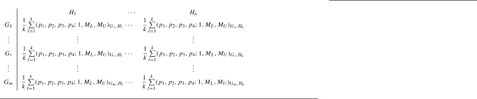
Let I be a fixed set of indices and R be the set of all real numbers. Let $G=\{G_1,G_2,\ldots ,G_m\},H=\{H_1,H_2,\ldots ,H_n\}\subset I$. The general form of multi-criteria decision making based on LIM $A_{\text {LIM}}$ is given as

where for every i, j $(1\le i\le m, 1\le j\le n): G_i$ is the object being evaluated and $H_j$ is the criterion taking part in the evaluation and ${\text {LT}}_{G_i, H_j}$ is a linguistic term.

By converting each linguistic term into fuzzy number, we get the general form of multi-criteria decision making based on FIM $A_{FIM}$ which is given as

The general form of Hexagonal Fuzzy Index Matrix (HXFIM) $[K,L,\{((h_1, h_2, h_3, h_4, h_5, h_6); u, u_L, u_R)_{k_i,l_j}\}]$, the general form of multi-criteria decision making $A_{HXFIM}$ based on HXFIM can be defined analogously.

Algorithm for group multi-criteria LIM

Let I be a fixed set of indices. Let $G=\{G_1,G_2,\ldots ,G_m\}, H=\{H_1,H_2,\ldots ,H_n\}\subset I$. Let ${\text {LIM}}_1, {\text {LIM}}_2, \ldots , {\text {LIM}}_k$ be linguistic index matrices given by multiple decision makers ${\text {DM}}_1, {\text {DM}}_2, \ldots , {\text {DM}}_k$. The algorithmic procedure for the group multi-criteria LIM $A_{{\text {LIM}}_1}, A_{{\text {LIM}}_2}, \ldots , A_{{\text {LIM}}_k}$ can be summarized as follows:

• 1. Form the group multi-criteria linguistic index matrix $A_{{\text {LIM}}_1}, A_{{\text {LIM}}_2}, \ldots , A_{{\text {LIM}}_k}$ given by multi-decision makers ${\text {DM}}_1, {\text {DM}}_2, \ldots , {\text {DM}}_k$.

• 2. Form the corresponding group multi-criteria Parabolic Fuzzy Index Matrix (PFIM)

  $A_{{\text {PFIM}}_1}, A_{{\text {PFIM}}_2}, \ldots , A_{{\text {PFIM}}_k}$ for the group multi-criteria linguistic index matrix $A_{{\text {LIM}}_1}, A_{{\text {LIM}}_2}, \ldots , A_{{\text {LIM}}_k}$ using the conversion Table.

• 3. The aggregated multi-criteria PFIM $A_{PFIM}$ of corresponding evaluations with respect to each decision makers of the given group multi-criteria PFIM by considering equal weights to all decision makers is found using the row average aggregation for given PFIM $[G,H,\{(p_1, p_2, p_3, p_4;1, M_{L}, M_{U})_{G_i,H_j}\}]$ defined by

  

  where $\sum$ is found using Definition 2.6.

• 4. The ranking of FNs/PFNs has not been uniquely defined in literature. But, a totally ordering principle has been defined on the entire class of generalized hexagonal fuzzy numbers in [43]. Hence, a ranking of two fuzzy numbers P and Q can be found by hexagonal approximation which is defined as $P\le Q$ if $\mathcal {H}(P) \le \mathcal {H}(Q)$ where $P = (p_1, p_2, p_3, p_4;1, M_{P_L}, M_{P_R})$ and $Q =(q_1, q_2, q_3, q_4;1, M_{Q_L}, M_{Q_R})$. Therefore, compute hexagonal approximation is in the form of LR representation and then convert it into general representation corresponding to each parabolic fuzzy numbers.

• 5. Find the score M using Definition 2.4 and if required S, LD, LA, RD, RA accordingly, to conclude whether $G_p > G_q$ or $G_p < G_q$ or $G_p=G_q$ for all $G_p, G_q \in U$.

• 6. Enumerate $E_A(G_p, G_q)$ using $E_A(G_p, G_q)=\{ a \in H | G_p > G_q\}$ and $F_A(G_p, G_q)$ using $F_A(G_p, G_q)=\{a \in H | G_p=G_q\}$. Compute the weighted fuzzy dominance relation using $WD_A(G_p, G_q):U \times U \rightarrow [0, 1]$ is defined by $WD_A(G_p, G_q)=\sum _{a \in E_A(G_p, G_q)}w_a+\frac{\sum _{a \in F_A(G_p, G_q)}w_a}{2}$.

• 7. Evaluate the entire dominance degree of each alternative using $D_A(G_p)=\frac{1}{|U|}\sum _{q=1}^{|U|}WD_A(G_p, G_q)$. The alternatives are ordered using entire dominance degree. The larger value of $D_A(G_p)$ is the best alternative.

Fig. 3

Flowchart of algorithm for group multi-criteria LIM

Table 6 Combined LIM $(A_{{\text {LIM}}_1}, A_{{\text {LIM}}_2})$

For the sake of simplicity, the algorithm for group multi-criteria LIM is given below as Fig. 3.

Numerical illustration

In the real-life environment, multi-criteria group decision-making problem includes imprecise, indefinite and subjective information from human judgement and preference. Fuzzy set theory provides the flexibility to deal such information. In this sub-section, a problem of supplier selection under group decision-making environment in which the evaluations of alternatives against each criterion are considered as linguistic variables is considered to show the applicability of the proposed hexagonal approximation.

A company with two decision makers ${\text {DM}}_1$, ${\text {DM}}_2$ of equal weightage has to select the best warehouse to export their manufactured goods for the sale based on cost, locality population, warehouses area, distance to warehouses, performance of alternatives. After some pre-screening, these alternatives (warehouses) $G_1, G_2, G_3, G_4, G_5, G_6, G_7, G_8$ remain for further evaluations under those decision makers based on the criteria $H_1$: cost, $H_2$ : locality population, $H_3$: warehouses area, $H_4$: distance to warehouses $H_5$: performance and weights for each criteria $w_a$ is given by $W=\{w_a | a \in H\}=\{0.28, 0.25, 0.12, 0.15, 0.20\}$. Let LIM be a combined linguistic index matrix given in Table 6 which consists of individual linguistic index matrices ${\text {LIM}}_1, {\text {LIM}}_2$ given by decision makers ${\text {DM}}_1, {\text {DM}}_2$.

Step 1 & 2: The conversion table of linguistic opinions of decision makers into parabolic fuzzy numbers is given in Table 7 and the group multi-criteria PFIM $(A_{{\text {PFIM}}_1}, A_{{\text {PFIM}}_2})$ is formed using Table 6 and is depicted in Table 8.

Table 7 The conversion table of linguistic opinions into PFNs

Table 8 The group multi-criteria PFIM $(A_{{\text {PFIM}}_1, {\text {PFIM}}_2})$

Table 9 Aggregated PFIM

Table 10 LR hexagonal approximation of PFIM

Table 11 General representation of hexagonal approximation

Step 3: The aggregated multi-criteria PFIM $A_{PFIM}$ with respect to each decision makers of the given group multi-criteria PFIM by considering equal weights to all decision makers is found and is tabulated in Table 9 using the Definition 2.6.

Step 4: The ranking of alternatives in the form of parabolic fuzzy numbers is not possible in the literature, hence it is required to approximate the parabolic fuzzy numbers without much loss of information. Therefore, compute hexagonal approximation is in the form of LR representation and then convert it into general representation corresponding to each parabolic fuzzy numbers (Tables 10, 11).

Step 5: Using Definition 2.4, the midpoint score M is found and is tabulated in Table 12. If $M(G_i/H_j)=M(G_j/H_j)$ for any alternatives $G_i, G_j$ then S and other necessary score functions LD, LA, RD and RA are found whenever required (Table 13).

Step 6: The weighted fuzzy dominance relation is evaluated and is depicted in Table 14. For instance $E_A(G_2, G_1)=\{H_2, H_4, H_5\}$ and $F_A(G_2, G_1)=\{ H_3\}$ and hence $WD_A(G_2, G_1)=0.25+0.15+0.20+0.06=0.660$.

Step 7: Now, the entire dominance degree of each alternative using $D_A(G_i)=\frac{1}{|U|}\sum _{j=1}^{|U|}WD_A(G_i, G_j)$ is found. For instance $D_A(G_2)=\frac{1}{8}\sum _{j=1}^{8}WD_A(G_2, G_j)=0.473750$.

By step 7 $G_6$ is selected as the best alternative from the above table (Table 15).

Conclusion and future scope

Even several defuzzification methods for fuzzy numbers exists in the literature, approximation of fuzzy numbers is the effective framework among them. We also have suggested a new approach of hexagonal approximation for fuzzy numbers. The propounded operator called the hexagonal approximation operator preserving the core possess many desired properties and less loss of information. Furthermore, the betterment from other approximation methods has also been discussed. Finally, the applicability of the proposed approximation method is described by MCDM problem using Index Matrix. Since any numerical data involved inthe research experiment of engineering problem can be fitted by quadratic fuzzy number which may be approximated into Hexagonal fuzzy number without affecting much information, this proposed method has a wide applications in all Engineering problems. In near future, this methodology can be extended to intuitionistic fuzzy numbers, neutrosophic fuzzy numbers, hesitancy fuzzy numbers and dual hesitancy fuzzy numbers by which MCDM may be studied and applied in many real-life applications where non-linear information plays a vital role. Therefore, it opens a new area of research of approximation of nonlinear fuzzy numbers by piecewise linear fuzzy numbers of different shapes and applications of different engineering and management problems.

Table 12 Score functions M, S, LD of HXFNs

Table 13 Score functions LA, RD, RA of HXFNs

Table 14 Weighted dominance relation

Table 15 Dominance relation

References

Abbasbandy S, Amirfakhrian M (2006) The nearest approximation of a fuzzy quantity in parametric form. Appl Math Comput 172(1):624–632
Abbasbandy S, Amirfakhrian M (2006) The nearest trapezoidal form of a generalized left right fuzzy number. Int J Approx Reason 43(2):166–178
Abbasbandy S, Asady B (2004) The nearest trapezoidal fuzzy number to a fuzzy quantity. Appl Math Comput 156(2):381–386
Adriana B (2011) Approximation of fuzzy numbers by trapezoidal fuzzy numbers preserving the core and the expected value. Studia Universitatis Babes-Bolyai, Mathematica 56(2)
Atanassov K (1987) Generalized index matrices. C R Acad Bulgare sci 40(11):15–18
Babu S, Thorani Y, Shankar NR (2012) Ranking generalized fuzzy numbers using centroid of centroids. Int J Fuzzy Logic Syst 2(3):17–32
Ban AI (2006) Nearest interval approximation of an intuitionistic fuzzy number. In: Computational intelligence, theory and applications. Springer, pp 229–240
Ban A (2008) Approximation of fuzzy numbers by trapezoidal fuzzy numbers preserving the expected interval. Fuzzy Sets Syst 159(11):1327–1344
Ban A (2008) Trapezoidal approximations of intuitionistic fuzzy numbers expressed by value, ambiguity, width and weighted expected value. Notes Intuition Fuzzy Sets 14(1):38–47
Ban AI (2009) On the nearest parametric approximation of a fuzzy number-revisited. Fuzzy Sets Syst 160(21):3027–3047
Ban AI (2009) Triangular and parametric approximations of fuzzy numbers-inadvertences and corrections. Fuzzy Sets Syst 160(21):3048–3058
Ban A, Coroianu L (2011) Translation invariance and scale invariance of approximations of fuzzy numbers. In: Proceedings of the 7th conference of the European society for fuzzy logic and technology. Atlantis Press, pp 742–748
Ban AI, Coroianu LC (2011) Metric properties of the nearest extended parametric fuzzy number and applications. Int J Approx Reason 52(4):488–500
Ban AI, Coroianu L (2012) Nearest interval, triangular and trapezoidal approximation of a fuzzy number preserving ambiguity. Int J Approx Reason 53(5):805–836
Ban AI, Coroianu L (2012) Weighted semi-trapezoidal approximation of a fuzzy number preserving the weighted ambiguity. In: International conference on information processing and management of uncertainty in knowledge-based systems, vol 299. Springer, pp 49–58
Ban AI, Coroianu L (2014) Existence, uniqueness and continuity of trapezoidal approximations of fuzzy numbers under a general condition. Fuzzy Sets Syst 257:3–22
Ban AI, Coroianu L (2015) Existence, uniqueness, calculus and properties of triangular approximations of fuzzy numbers under a general condition. Int J Approx Reason 62:1–26
Ban AI, Coroianu L (2016) Symmetric triangular approximations of fuzzy numbers under a general condition and properties. Soft Comput 20(4):1249–1261
Ban A, Brandas A, Coroianu L, Negrutiu C, Nica O (2011) Approximations of fuzzy numbers by trapezoidal fuzzy numbers preserving the ambiguity and value. Comput Math Appl 61(5):1379–1401
Ban AI, Coroianu L, Khastan A (2016) Conditioned weighted l-r approximations of fuzzy numbers. Fuzzy Sets Syst 283:56–82
Chakraborty A, Mondal SP, Alam S, Ahmadian A, Senu N, De D, Salahshour S (2019) The pentagonal fuzzy number: Its different representations, properties, ranking, defuzzification and application in game problems. Symmetry 11(2):248
Chakraborty A, Maity S, Jain S, Mondal SP, Alam S (2020) Hexagonal fuzzy number and its distinctive representation, ranking, defuzzification technique and application in production inventory management problem. Granul Comput:1–15
Chanas S (2001) On the interval approximation of a fuzzy number. Fuzzy Sets Syst 122(2):353–356
Coroianu L (2012) Lipschitz functions and fuzzy number approximations. Fuzzy Sets Syst 200:116–135
Coroianu L (2020) Trapezoidal approximations of fuzzy numbers using quadratic programs. Fuzzy Sets Syst. https://doi.org/10.1016/j.fss.2020.05.016
Coroianu L, Stefanini L (2015) A note on fuzzy-transform approximation of fuzzy numbers. In: 2015 Annual conference of the North American Fuzzy Information Processing Society (NAFIPS) held jointly with 2015 5th World Conference on Soft Computing (WConSC). IEEE, pp 1–6
Coroianu L, Stefanini L (2016) General approximation of fuzzy numbers by f-transform. Fuzzy Sets Syst 288:46–74
Coroianu L, Gal SG, Bede B (2014) Approximation of fuzzy numbers by max-product bernstein operators. Fuzzy Sets Syst 257:41–66
Coroianu L, Gagolewski M, Grzegorzewski P (2019) Piecewise linear approximation of fuzzy numbers: algorithms, arithmetic operations and stability of characteristics. Soft Comput 23(19):9491–9505
Delgado M, Vila MA, Voxman W (1998) A fuzziness measure for fuzzy numbers: Applications. Fuzzy Sets Syst 94(2):205–216
Dubois D, Prade H (1987) The mean value of a fuzzy number. Fuzzy Sets Syst 24(3):279–300
Garg H, Ansha (2018) Arithmetic operations on generalized parabolic fuzzy numbers and its application. Proc Natl Acad Sci India Sect A 88(1):15–26
Grzegorzewski P (2002) Nearest interval approximation of a fuzzy number. Fuzzy Sets Syst 130(3):321–330
Grzegorzewski P (2008) Trapezoidal approximations of fuzzy numbers preserving the expected interval–algorithms and properties. Fuzzy Sets Syst 159(11):1354–1364
Grzegorzewski P (2010) Algorithms for trapezoidal approximations of fuzzy numbers preserving the expected interval. In: Foundations of reasoning under uncertainty. Springer, pp 85–98
Grzegorzewski P, Mrówka E (2005) Trapezoidal approximations of fuzzy numbers. Fuzzy Sets Syst 153(1):115–135
Grzegorzewski P, Mrówka E (2007) Trapezoidal approximations of fuzzy numbers–revisited. Fuzzy Sets Syst 158(7):757–768
Grzegorzewski P, Pasternak-Winiarska K (2014) Natural trapezoidal approximations of fuzzy numbers. Fuzzy Sets Syst 250:90–109
Heilpern S (1992) The expected value of a fuzzy number. Fuzzy Sets Syst 47(1):81–86
Huang H, Wu C, Xie J, Zhang D (2017) Approximation of fuzzy numbers using the convolution method. Fuzzy Sets Syst 310:14–46
Khan NA, Razzaq OA, Chakraborty A, Mondal SP, Alam S (2020) Measures of linear and nonlinear interval-valued hexagonal fuzzy number. (IJFSA 9(4):21–60
Khastan A, Moradi Z (2016) Width invariant approximation of fuzzy numbers. Iran J Fuzzy Systs 13(2):111–130
Lakshmana Gomathi V, Nayagam JM, Suriyapriya K (2020) Hexagonal fuzzy number inadvertences and its complete ranking by score functions. Comput Appl Math (in Press)
Li S, Li H (2017) An approximation method of intuitionistic fuzzy numbers. J Intell Fuzzy Syst 32(6):4343–4355
Li S-y, Li H-x (2017) Trapezoidal intuitionistic approximations of intuitionistic fuzzy numbers preserving the width. In: International conference on fuzzy information & engineering. Springer, pp 3–10
Li S, Yuan X, Li H (2017) Approximation of intuitionistic fuzzy numbers by trapezoidal intuitionistic fuzzy numbers. J Intell Fuzzy Syst 33(1):389–402
Ma M, Kandel A, Friedman M (2000) A new approach for defuzzification. Fuzzy Sets Syst 111(3):351–356
Maity S, Chakraborty A, De SK, Mondal SP, Alam S (2020) A comprehensive study of a backlogging eoq model with nonlinear heptagonal dense fuzzy environment. Recherche Opérationnelle, RAIRO, p 54
Murugan Jagadeeswari, Nayagam VLG (2011) Trapezoidal approximation of neutrosophic numbers on transportation problems. J Adv Res Dyn Control Syst 11(6):377–394
Nayagam VLG, Jagadeeswari M (2017) Approximation of parabolic fuzzy numbers. FSDM 107–124
Nayagam VLG, Murugan J (2020) Triangular approximation of intuitionistic fuzzy numbers on multi-criteria decision making problem. Soft Comput:1–28
Nayagam VLG, Muralikrishnan S, Sivaraman G (2011) Multi-criteria decision-making method based on interval-valued intuitionistic fuzzy sets. Expert Syst Appl 38(3):1464–1467
Nayagam VLG, Ponnialagan D, Jeevaraj S (2019) Similarity measure on incomplete imprecise interval information and its applications. Neural Comput Appl:1–13
Nayagam V, Dhanasekaran P, Jeevaraj S (2016) A complete ranking of incomplete trapezoidal information. J Intell Fuzzy Syst 30(6):3209–3225
Nayagam VLG, Jeevaraj S, Dhanasekaran P (2016) A linear ordering on the class of trapezoidal intuitionistic fuzzy numbers. Expert Syst Appl 60:269–279
Nayagam VLG, Jeevaraj S, Dhanasekaran P (2017) An intuitionistic fuzzy multi-criteria decision-making method based on non-hesitance score for interval-valued intuitionistic fuzzy sets. Soft Comput 21(23):7077–7082
Nayagam VLG, Jeevaraj S, Sivaraman G (2017) Ranking of incomplete trapezoidal information. Soft Comput 21(23):7125–7140
Nayagam VLG, Jeevaraj S, Dhanasekaran P (2018) An improved ranking method for comparing trapezoidal intuitionistic fuzzy numbers and its applications to multicriteria decision making. Neural Comput Appl 30(2):671–682
Ponnialagan D, Selvaraj J, Velu LGN (2018) A complete ranking of trapezoidal fuzzy numbers and its applications to multi-criteria decision making. Neural Comput Appl 30(11):3303–3315
Velu LGN, Selvaraj J, Ponnialagan D (2017) A new ranking principle for ordering trapezoidal intuitionistic fuzzy numbers. Complexity
Wang G, Li J (2017) Approximations of fuzzy numbers by step type fuzzy numbers. Fuzzy Sets Syst 310:47–59
Wang Y-M, Yang J-B, Xu D-L, Chin K-S (2006) On the centroids of fuzzy numbers. Fuzzy Sets Syst 157(7):919–926
Yeh C-T (2008) On improving trapezoidal and triangular approximations of fuzzy numbers. Int J Approx Reason 48(1):297–313
Yeh C-T (2008) Trapezoidal and triangular approximations preserving the expected interval. Fuzzy Sets Syst 159(11):1345–1353
Yeh C-T (2017) Existence of interval, triangular, and trapezoidal approximations of fuzzy numbers under a general condition. Fuzzy Sets Syst 310:1–13
Yeh C-T (2018) Note on symmetric triangular approximations of fuzzy numbers under a general condition and properties. Soft Comput 22(7):2133–2137
Yeh C-T, Chu H-M (2014) Approximations by lr-type fuzzy numbers. Fuzzy Sets Syst 257:23–40
Zeng W, Li H (2007) Weighted triangular approximation of fuzzy numbers. Int J Approx Reason 46(1):137–150
Acknowledgements
The Authors thank the anonymous referees and editors for their valuable suggestions and queries which improved the quality of the paper. This work was supported by UGC-Rajiv Ganhi National Fellowship Scheme (RGNF-2014-15-SC-TAM-74350).
Author information
Authors and Affiliations
Corresponding author
Ethics declarations
Conflict of interest
The authors declare that there is no conflict of interest. This article does not contain any studies with human participants or animals performed by any of the authors. The authors ensure that they have written entirely original works based on their own research, and if the authors have used the work and/or words of others, this has been appropriately cited or quoted with the best of their knowledge.
Additional information
Publisher's Note
Springer Nature remains neutral with regard to jurisdictional claims in published maps and institutional affiliations.
Rights and permissions
Open Access This article is licensed under a Creative Commons Attribution 4.0 International License, which permits use, sharing, adaptation, distribution and reproduction in any medium or format, as long as you give appropriate credit to the original author(s) and the source, provide a link to the Creative Commons licence, and indicate if changes were made. The images or other third party material in this article are included in the article’s Creative Commons licence, unless indicated otherwise in a credit line to the material. If material is not included in the article’s Creative Commons licence and your intended use is not permitted by statutory regulation or exceeds the permitted use, you will need to obtain permission directly from the copyright holder. To view a copy of this licence, visit http://creativecommons.org/licenses/by/4.0/.
About this article
Cite this article
Nayagam, V.L.G., Murugan, J. Hexagonal fuzzy approximation of fuzzy numbers and its applications in MCDM. Complex Intell. Syst. 7, 1459–1487 (2021). https://doi.org/10.1007/s40747-020-00242-4
Received:
Accepted:
Published:
Issue Date:
DOI: https://doi.org/10.1007/s40747-020-00242-4