
Abstract
Convolutional neural networks (CNNs) exhibit state-of-the-art performance while performing computer-vision tasks. CNNs require high-speed, low-power, and high-accuracy hardware for various scenarios, such as edge environments. However, the number of weights is so large that embedded systems cannot store them owing to their limited on-chip memory. A different method is used to minimize the input image size, for real-time processing, but it causes a considerable drop in accuracy. Although pruned sparse CNNs and special accelerators are proposed, the requirement of random access incurs a large number of wide multiplexers for a high degree of parallelism, which becomes more complicated and unsuitable for FPGA implementation. To address this problem, we propose filter-wise pruning with distillation and block RAM (BRAM)-based zero-weight skipping accelerator. It eliminates weights such that each filter has the same number of nonzero weights, performing retraining with distillation, while retaining comparable accuracy. Further, filter-wise pruning enables our accelerator to exploit inter-filter parallelism, where a processing block for a layer executes filters concurrently, with a straightforward architecture. We also propose an overlapped tiling algorithm, where tiles are extracted with overlap to prevent both accuracy degradation and high utilization of BRAMs storing high-resolution images. Our evaluation using semantic-segmentation tasks showed a 1.8 times speedup and 18.0 times increase in power efficiency of our FPGA design compared with a desktop GPU. Additionally, compared with the conventional FPGA implementation, the speedup and accuracy improvement were 1.09 times and 6.6 points, respectively. Therefore, our approach is useful for FPGA implementation and exhibits considerable accuracy for applications in embedded systems.
1 Introduction
Convolutional neural networks (CNNs) [27] deliver state-of-the-art performance in computer-vision tasks such as object classification [25], object detection [30], and semantic segmentation [41]. They are increasingly required in a variety of embedded systems such as robots [48], self-driving cars [4], and drones [40]. The major problem is that CNNs involve so many parameters (especially weights) that resource-constrained embedded hardware cannot store them in on-chip memory. However, accessing the off-chip memory leads to low performance. Another approach is to use a high-bandwidth off-chip DRAM, such as a GPU. However, this causes considerable power dissipation and it exceeds the power consumption limit on an embedded system.
To address this problem, several network compression techniques have been proposed [8, 13, 18]. Pruning [13] is a compression technique that eliminates unnecessary weights below a threshold, where pruning converts dense weight matrices to unstructured sparse matrices. This approach can lead to more than a 10-fold reduction in the number of parameters with comparable accuracy [13]. However, such unstructured sparse matrices lead to inefficient use of the underlying hardware resources. The main reason is that the distribution of non-zero weights is extremely skewed, which leads to imbalanced loading among processing elements (PEs). In summary, although pruning with no constraints reduces memory usage, the imbalance decreases the efficiency of hardware performance.
Several studies have proposed special accelerators for sparse CNNs. Cambricon-X [52] allowed different PEs to load new data from the memory asynchronously to improve the overall efficiency. SCNN [37] used Cartesian product-based processing with many memory banks for sparse convolutional layers, and STICKER [51] applied two-way set associative PEs to SCNN architecture to reduce the memory area to 92%. To deal with the load imbalance problem, some accelerators introduced very wide memory and multiplexers (MUXs), becoming more complex. For example, Cambricon-X [52] is a MUX-based accelerator, and the MUXs occupy more than 30% of the total chip area. This means that this architecture is unsuitable for FPGA implementation because MUXs are particularly area-intensive, with an area ratio greater than 100 × than those of custom CMOS circuits [46].
A new algorithm/hardware co-design approach is proposed in this study. It involves filter-wise pruning with distillation, and its special inter-layer pipelined accelerator for FPGA implementation. In the pruning step, filter-wise pruning eliminates weights such that each filter has the same number of nonzero weights, which resolves the imbalanced loading problem naturally. At the retraining step, the remaining weights are retrained with a distillation technique, where dense and sparse networks serve as the teacher and the student, respectively. The use of the dense network’s training information increases the accuracy of the sparse network and accelerates training convergence. As for hardware architecture, we developed a zero-weight skipping inter-layer pipelined accelerator. While the conventional sparse CNN accelerator is a multiplexer-based architecture, our accelerator is a BRAM-based architecture for random access to corresponding input feature maps. Thus, our accelerator does not load invalid feature maps from memory. In addition, because each filter has the same number of nonzero weights, utilizing inter-filter parallelism does not require complicated functions. Thus, our architecture achieves a high degree of parallelism with simple hardware complexity.
This paper is an extended version of our previous work [42], in which we improved filter-wise pruning with distillation and its special accelerator on an FPGA. In this work, we apply our filter-wise pruning with distillation to a lightweight network model, MobileNetV1-based model, and compare it with the state-of-the-art FPGA implementation. To deal with high-resolution images, we also propose an overlapped tiling algorithm where tiles are extracted with overlap to prevent accuracy drop. With conventional optimization techniques, our achieved latency and accuracy surpassed the best previously FPGA implementation by 1.09 times and 6.6 points, respectively.
Some of the contributions of our previous work [42] are detailed below.
-
1.
We suggested an AlexNet-based sparse fully convolutional network (SFCN) on an FPGA. While our model had fewer parameters and a significantly smaller network than conventional models, it has high accuracy in practice.
-
2.
We proposed a filter-wise pruning technique that sorts weight parameters by their absolute values and then prunes them by a preset percentage from a small order (Section 4). Our technique realizes a higher sparse model than previous work [13], without degrading the accuracy.
-
3.
We compared our system on an FPGA and a mobile GPU in terms of speed, power, and power efficiency. As for frame per second (FPS), the FPGA realization is 10.14 times faster than that of the GPU.
The new contributions of our new study are as follows:
-
1.
Instead of the AlexNet-based SFCN, we propose a MobileNetV1-based PSPNet, which is an efficient lightweight network model (Section 7.1) with higher accuracy. We show that our pruning makes even a lightweight model more hardware-aware without significantly degrading the accuracy (Section 7.3).
-
2.
We propose an overlapped tiling algorithm to reduce the utilization of on-chip memory on FPGAs for high-resolution images (Section 6). The overlap with appropriate strides relieves the high utilization problem of BRAMs, while maintaining the original accuracy.
-
3.
Conventional optimization techniques, such as 8-bit integer quantization and batch normalization folding are adopted (Section 3.2). In addition, the previous FPGA-based accelerator in ARC 2019 is expanded to use inter-filter parallelism (Section 5.1). These optimizations make our accelerator faster.
-
4.
We compare our filter-wise pruned MobileNetV1-based PSPNet with the state-of-the-art network using cityscape dataset (Section 7.5). We illustrate that our implementation outperforms the existing implementation for both the GPU and FPGA.
The rest of the paper is organized as follows: the motivation for our work is presented in Section 2. The terminology thoroughly used in this paper is explained in Section 3. A novel pruning technique, filter-wise pruning with distillation, and its special accelerator are described in Sections 4 and 5, respectively. The proposed overlapped tiling algorithm for high-resolution images is explained in Section 6. Our implementation is compared with the previous state-of-the-art works in Section 7, and Section 8 explains how it is different from conventional works. The conclusion is presented in Section 9.
2 Motivation
2.1 Unstructured Nonzero Weight Matrices
Pruning is frequently used to reduce the number of weights for CNN implementation in resource-constrained embedded hardware. The procedure of the typical pruning technique [13] is as follows:
-
1)
Train the network weights
-
2)
Prune the small weights below a threshold
-
3)
Retrain the remaining weights
After pruning, most weights become zero; the weights are stored in a format, such as the coordinate (COO) format or the compressed sparse row (CSR) format. As an example, we consider the pseudo-code shown in Fig. 1 for sparse convolution (CONV) with the COO format. The code consists of four loops. In each loop, a weight and an address (row, column, and channel values) are loaded, and the multiply accumulate (MAC) operation is performed as many times as the number of non-zero weights. We categorize parallelism into the following different types based on the unrolling strategies.
-
1.
Spatial Parallelism, where loop L2, loop L3, or both are unrolled
-
2.
Inter-filter parallelism, where loop L1 is unrolled
-
3.
Intra-filter parallelism, where loop L4 is unrolled

Pseudo-code of sparse CONV with the COO format.
In order to realize high-speed calculation, the three types of parallelisms mentioned above must be flexibly utilized based on network architectures.
Figure 2 depicts the nonzero-weight ratio of each pruned filter in MobileNetV1 [19]. There is a significant difference in the nonzero-weight ratios between a certain pair of filters. Similar to the case in the example, certain pruned networks have highly skewed nonzero-weight distributions [28]. This imbalance makes it more difficult to utilize inter- and intra-filter parallelisms. However, changing the distribution of nonzero weights would delete weights with big magnitudes, leading to accuracy degradation. In detail, one of the methods for reducing the imbalance is coarse-grained pruning, block pruning. Shijie Cao et al. reported that although the imbalance is released, block pruning only preserves less than half of the weights with big magnitude [5]. From the viewpoints of hardware efficiency, Cambricon-S [56] shows that reduction in the imbalance leads that one not multiple shared neuron selector module is sufficient, saving 10.35 mm2 area and 1821.9 mW power consumption. In addition, the reduction reduces the memory accesses of weight indices by 26.83 × and achieves 1.11 × better energy efficiency. The balance of accuracy and hardware efficiency is one of the research problems. To resolve this problem, we have equalized the number of nonzero weights of each filter during the training phase. This equalization makes it easier to exploit the underlying inter- and intra-filter parallelisms without complicated techniques and accuracy degradation.

The non-zero weight ratio of pruned filters in the first layer in our MobileNetV1. The layer has 32 filters, and the sparse ratio is set 94%.
3 Background
3.1 Convolutional Neural Networks
3.1.1 Convolution (CONV)
Figure 3 illustrates CONV. Let Xi(w,h,ch) be an input feature map (IFM) value at (w,h,ch) coordinates in i-th layer, Wi(r,c,ch) be a weight value, wbias be a bias, Si(w,h) be an intermediate variable, fact(x) be an activation function, and Xi+ 1(w,h) be an (i+ 1)-th IFM, or i-th output feature map (OFM). The K × K 2D CONV at (w,h) coordinates in (i + 1)-th layer is as follows:
where N is the i-th IFM channel, r, c, and ch are coordinates of width-axis, height-axis, and channel-axis, respectively. The input is multiplied by a weight and the resulting sum is applied to the activation function. In this paper, we use the rectified linear unit (ReLU) functions as the activation function. When K = 1 (or pixel-wise CONV), it plays the role of classification corresponding to the part of input images.

CONV.
3.1.2 Separable CONV
Because conventional CNNs [15, 25, 43] have much redundancy, light-weight CNNs have been proposed [6, 19, 47, 49]. Among them, separable CONV proposed in MobileNetV1 reduces a lot of weight parameters by factorization in spatial dimension. Figure 4 shows separable CONV. Separable CONV consists of a depthwise CONV (DwCONV) and a pointwise CONV (PwCONV). The DwCONV computes OFMs only from a single input channel (each CONV is independent of the channel-axis), and the PwCONV is a 1 × 1 conventional CONV. The computational cost of a conventional CONV in terms of both multiplication and addition is as follows:
where M is OFM channel. On the other hand, The cost of the separable CONV can be computed as follows:

Separable CONV.
By converting the typical conventional K × K CONV to the separable CONV, the computational cost can be reduced. Typically, because K2 ≪ M(e.g. K = 3 and M = 256), the computational cost is reduced approximately by a factor of K2 = 9.
3.1.3 Sparse CONV
After a pruning technique is applied, many weight values become zero. To store such weight parameters formed in the sparse matrix to memories efficiently, we employ a coordinate (COO) format. The arrays, row, col, ch, and weight store its row, column, channel indices, and nonzero-weights of the sparse matrix, respectively. Since pruning realizes a high-sparse matrix, the overhead of additional memory requirement (row, col, and ch arrays) is not critical. When COO format is introduced, the sparse CONV at (w,h) coordinates is formulated as follows.
where N is the number of nonzero-weights, wj is a weight value, and colj and rowj are column and row indices, respectively.
3.2 Inference Optimization
3.2.1 Batch Normalization Folding
In order to accelerate training time and convergence, the CNN is first learned by a set of training data (mini-batch). Since various distributions of each mini-batch cause internal covariate shifts that can lengthen learning time, it is necessary to carefully determine the initial parameter values. To solve the costs, batch normalization (BN) [20] is often used as shown in the following:
where g is a batch size, xi is an i-th mini-batch input, μ is a mini-batch mean value, \({\sigma ^{2}_{B}}\) is a mini-batch variance, and 𝜖 is a hyper parameter. γ and β are learning parameters that change at the learning phase. At inference, γ and β is constant value, and then the batch normalization is expressed as:
where \(\gamma ^{\prime } = \frac {\gamma }{\sqrt {{\sigma ^{2}_{B}}+\epsilon }}\) and \(\beta ^{\prime } = \beta -\frac {\gamma \mu _{B}}{\sqrt {{\sigma ^{2}_{B}}+\epsilon }}\). Next, this BN calculation is folded into CONV calculation.
where \(W^{\prime }(r,c,ch) = \gamma ^{\prime } \cdot W(r,c,ch)\) and \(w^{\prime }_{bias} = \gamma ^{\prime } \cdot w_{bias} + \beta ^{\prime }\). This conversion hides BN overhead completely.
3.2.2 8-Bit Integer Quantization Scheme
Some studies show that 8-bit quantized neural networks maintain accuracy, compared with floating-point precision [21, 24]. Because quantization allows inference to be carried out using integer-only arithmetic, hardware can equip more mathematical computation cores, leading to speedup. The quantization scheme (scale+shift quantization) converted from quantized parameters to real number is obtained as follows:
where r is a real value, S is a positive real value (scale value), and q is a quantized value, or an 8-bit integer value in this study. Z is the quantized value corresponding to real value 0 (shift value), round(⋅) is a rounding function to the nearest integer, and a,b is a valid range of real values [a,b]. When Z is a non-zero value, matrix multiplication with the quantization scheme incurs calculation overhead [21]. Thus, scale quantization is often used, as shown below.
This quantization scheme is applied after BN folding. In addition, quantization-aware training is often required because post-quantization may incur accuracy degradation. During training, the valid range [a, b] changes in accordance with the input batches, and the min/max statistics or moving average of the min/max values are used to compute the range.
This paper uses scale quantization scheme to convert to integer precision. Since our used networks contain ReLU function, the ranges of weights and activations are different: activations are converted into unsigned integer precision, and weights are integer precision. Additionally, the valid range [a, b] is calculated by moving average of min/max values since min/max statistics approach may occur accuracy degradation due to outliers. Using the decided range, the scale value is calculated as follows:
If some values surpass the valid range, saturating cast is used.
3.3 Semantic Segmentation
Semantic segmentation is a fundamental task in image processing, in which pixel-wise classification is performed, as shown in Fig. 5. In this study, semantic segmentation tasks are performed to evaluate our proposal. Three performance metrics are employed here. Let nij be a #pixels of class i predicted as class j, and nclass is a number of classes to recognize. The metrics are as follows:
- Pixel-wise accuracy (Pixel-wiseAcc)::
-
$$ \begin{array}{@{}rcl@{}} \frac{{\sum}_{i=1}^{n_{class}}n_{ii}}{{\sum}_{i=1}^{n_{class}}{\sum}_{j=1}^{n_{class}}n_{ij}} = \frac{Accurate area}{All area}. \end{array} $$(12)
- Mean class accuracy (mClassAcc)::
-
$$ \frac{1}{n_{class}}\sum\limits_{i=1}^{n_{class}}\frac{n_{ii}}{{\sum}_{j=1}^{n_{class}}n_{ij}} = \frac{Area predicted as class i}{Truth area of class i}. $$(13)
- Mean intersection over union (mIoU)::
-
$$ \begin{array}{@{}rcl@{}} \frac{1}{n_{class}}\sum\limits_{i=1}^{n_{class}}\frac{n_{ii}}{{\sum}_{j=1}^{n_{class}}(n_{ij} + n_{ji}) - n_{ii} }. \end{array} $$(14)

Semantic segmentation using the Cityscapes dataset [7].
4 Filter-Wise Pruning with Distillation
In this study, a method is presented involving filter-wise pruning with distillation. It consists of two steps: filter-wise pruning and retraining with distillation. The procedure is detailed below:
-
1)
Train network weights
-
2)
Sort the trained weights of each filter by their absolute values
-
3)
Prune the small weights using a preset percent filter-by-filter
-
4)
Retrain the remaining weights with distillation
By following the above procedure, each filter achieves the same sparse ratio, which simplifies the pruned-CNN accelerator. It can be observed that both the retraining time does not differ from conventional pruning [13]. The distillation scheme is detailed in the next section.
4.1 Distillation Scheme for Retraining Weights
Distillation [18] is a compression technique, where a network (student network) is trained using the outputs of a larger network (teacher network) to imitate the same outputs. The outputs of a teacher network are used to improve the accuracy of a smaller student network. This study exploits this concept to obtain a highly sparse network while maintaining accuracy. It accelerates the convergence while increasing the accuracy of the sparse network. Figure 6 presents an outline of the distillation scheme with the MobileNetV1-based network that we have used. We assign a dense network as the teacher and a sparse network as the student. The training objective function Ltrain is written as
where M is the number of connections between the teacher and the student networks (this paper sets M = 15), β is a hyper-parameter to balance their losses. \(L^{m}_{soft}\) is the m-th mean squared loss using both the network’s feature map (FM), and Lhard is the pixel-wise cross entropy loss using ground truth. \(L^{m}_{soft}\) is defined by

Distillation scheme.
where αm is a hyper parameter to balance their losses, Wi,Hi, and CHi indicate the i-th FM’s width, height, and channel. \({X^{i}_{s}}(w,h,ch)\) and \({X^{i}_{t}}(w,h,ch)\) are the i-th FM values at (w,h,ch) in the student and the teacher networks, respectively. Lhard changes by a task, and in this paper we employ a semantic segmentation task for evaluation. Therefore, Lhard is pixel-wise cross entropy loss and defined by
where Hin and Win denote input image size, σ(w,h,ch) is predicted class probabilities, and p(w,h,ch) ∈{0,1} is the ground truth class probabilities at (w,h,ch) coordinates.
5 Hardware Implementation
The overall architecture is presented in Fig. 7. The design consists of buffer parts for parameters and the convolutional block (CB) parts, which constitute the inter-layer pipelined architecture. A combination of filter-wise pruning and inter-layer pipelining enables a high degree of parallelism, together with architectural simplicity because each layer has only one filter loop count. All parameters, including weights and biases, were loaded into on-chip buffers from DDR3 memory. Thereafter, the processor sends an input image to the design, and CONV operations are performed in the first CB. The output feature maps are sent to the ping-pong buffer in the next CB to be read to compute the next layer operation. Finally, the outputs of the last CB are sent to the ARM processor. Weight matrices are stored in the on-chip memory in the COO format.

Overall architecture.
5.1 Convolutional Block
The architecture and functionality of a convolutional block (CB) are depicted in Figs. 8 and 9. This comprises of a COO decoder, COO counter, counter for convolutional operation, ping-pong buffer for feature maps (FMs), processing element (PE) for both down-scaling and ReLU, and MAC units. All the calculations in the CBs are in the integer precision.

Convolutional block architecture.

Functionality of our convolutional block.
The COO counter counts the number of non-zero weights of each filter; the COO decoder obtains the number and outputs the corresponding relative address, row, column, and channel values. Subsequently, to fetch the FM values, the absolute address is calculated using both the relative address and the convolutional counter, which indicates the coordinates where the CONV operation is performed. Figure 10 presents an example of the functionality. The CONV coordinates are (w,h) = (1,1), and the relative address is (row,col,ch) = (1,2,0). Therefore, the absolute coordinates of the corresponding FM values are (w + row,h + col,ch) = (2,3,0). The fetched value and the weight are fed into a multiply accumulate (MAC) unit, followed by PE for down-scaling and ReLU. In down-scaling, the type of quantized accumulated value is a 32-bit integer and converted by using the following equation:
where x is an accumulated value in a 32-bit integer; Sact, Sx, and Sw, are scales of activations, inputs, and weights, respectively; and \(S^{\prime } = \frac {S_{act}}{S_{x} S_{w}} \cdot 2^{31}\) is a shifted scale from the quantized accumulated value to activation. To avoid fixed point calculation, \(\frac {S_{act}}{S_{x} S_{w}}\) is shifted in advance to be a 32-bit integer, and scaled accumulated values are shifted to the right followed by the ReLU function. Finally, the output is stored in the next ping-pong buffer in the next CB.

Absolute and relative coordinates. The CONV counter has the absolute coordinates of the top-left pixel in the kernel, such as (w,h) = (1,1) and the COO decoder contains relative coordinates (row,col,ch) = (1,2,0).
This work employs spatial and inter-filter parallelisms to achieve a high degree of parallelism. For spatial parallelism, memory interleaving by array partitioning is used along the width axis of the IFM. The degree of inter-filter parallelism is 2 to avoid an increase in area overhead because the maximum number of BRAM ports is 2 when the BRAM configuration is set to the true dual-port mode. From two coordinates of nonzero weights in a certain pair of filters, several successive FM values along the width axis are fetched and sent simultaneously. The corresponding weights are broadcast to the corresponding MAC units. For the COO indices, we used true dual-port BRAMs as COO index buffers to read two corresponding indices in one cycle.
6 Overlapped Tiling Algorithm
Our accelerator is built based on BRAM-based architecture, and its BRAM utilization depends on the resolution of the input images. Therefore, when input images have high resolution, our accelerator requires a massive amount of BRAMs. To prevent this problem, we propose an overlapped tiling algorithm, as shown in Fig. 11. This method splits full-resolution images into a stream of small tiles, and the FPGA accelerator operates the layer calculations for cropped small images. It facilitates optimization of on-chip memories as a benefit of the small-sized tile images but not low-resolution images. A proposed deeply pipelined architecture processes a large number of tile images with low latency. Now, we assume that Hin and Win are the height and width of the incoming full-resolution image, respectively; Wt represents the tile resolution; and Sh,Sw represent the strides to crop from the full-resolution image. The details of the proposed technique are as follows:
-
1)
The incoming RGB images are split into smaller tiles by cropping with the (Wt,Wt) window and (Sh,Sw) stride. Thus, the tiles are cropped with overlapping pixels Wt − Sh and Wt − Sw along the y-axis and x-axis, respectively. The maximum stride to obtain the minimum split of the tiles is then represented as follows:
$$ \begin{array}{@{}rcl@{}} (S_{h}, S_{w})=\left( \left\lceil \frac{H_{in}-W_{t}}{\lceil \frac{H_{in}}{W_{t}} \rceil -1} \right\rceil, \left\lceil \frac{W_{in}-W_{t}}{\lceil \frac{W_{in}}{W_{t}} \rceil -1} \right\rceil \right). \end{array} $$(19)Given that a small Wt is selected, the recognition accuracy is reduced because it becomes difficult to capture a specific object in one tile.
Figure 11 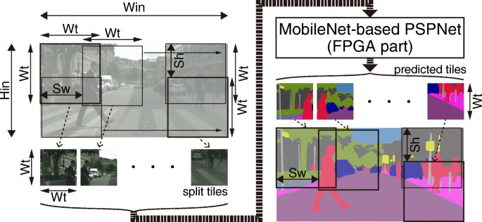
Proposed tile segmentation scheme.
-
2)
A network processes the split tiles on the pipelined architecture and outputs the predicted tiles that represent tens of label probabilities.
-
3)
The host processor reconstructs the predicted tiles into an image that is the same size as the input (Hin,Win) with the same strides (Sh,Sw), while the overlapped area is computed as an average. Finally, the full resolution of the predicted result is obtained.

In this paper, this tiling algorithm runs on processing system (PS) side in an FPGA.
7 Experimental Results
To evaluate the performance of our model and its implementation, we used the Chainer [44], which is a deep learning framework and the Cityscapes dataset [7], which is a popular dataset for semantic segmentation tasks. For FPGA implementation, we used HLS tools, SDSoC 2018.2 to convert C++ codes. The used FPGA board was a Xilinx Inc. Zynq UltraScale+ MPSoC zcu102 evaluation one, equipped with a Xilinx Zynq UltraScale+ MPSoC FPGA (ZU9EG, 68,520 Slices, 269,200 FFs, 1,824 18Kb BRAMs, 2,520 DSP48Es).
7.1 MobileNetV1-Based PSPNet
The CNN, MobileNetV1-based Pyramid Scene Parsing Network (PSPNet) [53] is presented in Table 1. Because the original PSPNet contains ResNet that consists of 101 layers, it cannot satisfy real-time processing requirements even in the case of desktop GPUs. To reduce the computation time and the number of parameters, we adopted MobileNetV1 as a feature extractor. The MobileNetV1-based model achieves similar accuracy and reduces model size, compared to state-of-the-art real-time segmentation networks [39, 55]. We eliminated 83% of the redundant weight,
7.2 Tradeoff for Various Tile Sizes
We analyzed the mIoU with various tile sizes to determine the optimal tile size in 32-bit floating models. We set the stride value (Sh,Sw) in order to achieve at least 25% overlap. Table 2 shows the accuracy for various tile sizes. When the tile size changed from 224 to 192, the accuracy dropped by 1.8 points significantly. The mIoU of the tile size 224 was 65.0%, which decreased by only 1.2 points from that of 1024 × 512. From the viewpoints of as smaller a size as possible with comparable accuracy, we chose a tile size of 224 × 224 for the 1024 × 512 images.
7.3 Accuracy Comparison for Sparseness Ratio and Quantization
We evaluated the difference between accuracies among the 32-bit floating model, 8-bit integer model, and 8-bit integer sparse model. We set the tile size as 224, and Table 3 exhibits the results of the accuracy comparison. The 8-bit quantization reduced the weight size by a factor of four with no accuracy drop from the float 32-bit precision. Compared with the 8-bit model, the sparse model reduced the number of multiple operations per tile by a factor of 10.4 with an accuracy drop of 0.9 points. In addition, the weights decreased by a factor of 22.8, and the number of MAC operations by a factor of 5.8. Thus, the combination of the overlapped tiling algorithm, filter-wise pruning, and conventional quantization achieved significant reduction in weight sizes and the number of multiple operations.
7.4 Comparison with a Desktop GPU
We compared our FPGA-based system with a GPU-based system that consists of the RTX 2080 Ti and Intel Core i7-7700 CPU. In GPU inference, we used PyTorch [38] using CUDA 11.0, CUDNN 8.0, and TensorRT 7.1 [36]. In power measurement, the CPU and the other peripheral devices are included in both the FPGA and GPU systems. As shown in Table 4, power efficiency of our FPGA system was 4.1 times higher than that of the GPU. This demonstrated that our specific architecture for the filter-wise pruning achieved high efficiency of valid computation. Thus, our FPGA system meets real-time processing requirements and has low power consumption, which means our system is highly suitable for embedded systems.
7.5 Comparison with Other FPGA Implementation
Table 5 compares our method to the previous state-of-the-art FPGA implementation [11].Footnote 1 Our model in a 512 × 256 system was 3.26 × faster with 7.0 points dropped mIoU, and 1.09 × faster with 6.6 points improved mIoU for a 1024 × 512 system. Our approach decreased accuracy in lower resolutions, while the maintained speed with high accuracy for higher resolutions. We considered that degradation is led by sparse models and tiling low-resolution images. In speed, although overlapped tiling increases the number of operations, ours for high resolutions achieved speedups. This means that proper coarse-grained units of pruning can delete a massive amount of both weights and operations. In power efficiency, power consumption was worse than the prior ones despite implementing our model with all on-chip memory. We considered that [11] used a custom-designed board with only minimal devices, while our work measured the total board power of the ZCU102 evaluation board including the peripheral devices, which means that the static power consumption of the peripheral devices leads to high power consumption. As a result, our system achieved the most accurate and fastest segmentation for the general dataset utilizing a large amount of on-chip memory and high-resolution image.
7.6 Comparison with Other Pruning Method
Finally, our filter-wise pruning with distillation was compared with the state-of-the-art coarse-grained pruning, filter pruning [17] that prunes filters with relatively less importance. Table 6 shows the comparison results with images in 512 × 224 size. Our proposal exceeded the accuracy of the filter pruning by 28.2 points. We considered that since in filter pruning the unit of pruning is big, a high sparse ratio affects accuracy significantly. Our approach provides fewer constraints with pruning, leading to a reduction in a massive amount of weights without significant accuracy degradation.
8 Related Works
8.1 Sparseness Approach for Weight Memory Reduction
Several pruning techniques have been proposed, comprising two types of pruning: unstructured and structured.
In unstructured pruning, the objective is to prune as many weights as possible without significantly degrading the accuracy degradation and any constraints. The representative method is deep compression [13], which combines quantization, weight pruning, and Huffman coding method to achieve a 3–4× speedup. Zhu and Gupta [57] proposed a gradual pruning method that increases the weight pruning ratio using a binary mask variable. In [34], various sparse dropout strategies were used for both fully connected and convolutional layers to realize high sparsity, and in [2], the rank of the parameter matrix in each layer was reduced.
While unstructured pruning can eliminate more weights than that of structured pruning, hardware cannot efficiently process imbalanced non-zero weight distribution. Structured pruning aims to prune weights with some constraints so that the resulting pruned networks become hardware-friendly topology. For the hardware of SIMD architecture, [50] proposed a SIMD-aware weight pruning that prunes by block-level to allow SIMD architecture to execute high parallelism for FC layers. Block pruning [12, 35] eliminates blocks of a weight matrix instead of individual weights. Block-wise pruning [5, 22, 23] prunes weights such that the number of non-zero weights in each block is equal. Channel pruning [10, 16, 31] prunes a certain filter that meets a condition. Finally, kernel-level and vector-level pruning [33] prunes kernels and vectors in kernels.
We propose a structured pruning, filter-wise pruning with distillation that eliminates weights filter-by-filter by a preset percentage. Filter-wise sparsity is a bigger unit among all conventional structured block-wise pruning techniques, which means that our proposal can preserve in more sparsity patterns.
8.2 FPGA Implementation for CNN-Based Semantic Segmentation
The CNN approach for semantic segmentation achieved state-of-the-art accuracy, and its first proposal is a fully convolutional network (FCN) [41]. FCN generates a coarse label map from input images by a pixel-wise classification, and the map is resized into the input image size by a bi-linear interpolation. Subsequently, we obtain a more fine-grained label map. SegNet [3] incorporates skip connections during deconvolution to improve the performance of small objects using middle-level features. The pyramid scene parsing network (PSPNet) [54] adopts a pyramid pooling module that applies pyramid pooling to feature maps, extracts features from them, and concatenates their futures to deal with multi-scaling objects. In addition, PSPNet uses the resizing function provided by OpenCV as an upsampling layer. ICNet [55] uses various resolution inputs to go through the corresponding networks and combine them using a cascade feature fusion unit.
These networks are not suitable for embedded systems because of their network size and complexity. Thus, some studies proposed specific lightweight networks [11, 32] for semantic segmentation to be implemented on an FPGA. Lyu et al. [32] proposed a small network for road segmentation with light detection and ranging (LiDAR), and its FPGA implementation meets a real-time processing requirement (59.2 FPS). In exchange for the FPGA realization by the proposed small model, it can deal with road class only, and therefore the implementation challenges of the task for many categories still remain. Fang et al. [11] proposed a feature pyramid network (FPN)-based and its accelerator for both object detection and semantic segmentation.
In this study, we present an AlexNet-based FCN and MobileNetV1-based PSPNet for implementation on FPGAs. The resulting model is a feed-forward architecture model, where there are no skip connections and no deconvolution layers, but resizing (bilinear interpolation) functions as upsampling layers. These conversions do not require the circuitry to have their IFM/OFM buffers, but memory access decreases significantly with low accuracy degradation. For these reasons, our proposed network is more suitable for embedded systems.
8.3 Sparse Convolutional Network Architecture
Our sparsity approach has attracted increasing interest because it reduces the data footprint and eliminates computation, and it achieves a good balance between the compression ratio and accuracy. Three types of architectures are outlined below, based on the values that are skipped: weights, activations, and both.
8.3.1 Zero-Weight Skipping Architecture
Zero-weight skipping architecture eliminates zero-weight calculations only. Cambricon-X [52] allows weight buffers in different processing elements to load new data from the memory asynchronously to improve the overall efficiency, since the numbers of weights of different neurons may differ significantly. J. Li, et al. [28] proposed a concise convolution rule (CCR) that decomposes sparse kernels into multiple effective nonzero sub-kernels using triplet representation.
8.3.2 Zero-Activation Skipping Architecture
Zero-activation skipping architecture eliminates zero-activation calculations only. The CNVLUTIN [1] architecture skips zero-activation multiplications, thereby improving both performance and energy efficiency.
8.3.3 Zero-Weight and -Activation Skipping Architecture
In zero-weight and -activation skipping architecture, all inefficient computations are eliminated. The EIE [14] exploits both sparsity and the indexing overhead. PermDNN [9] outperformed the EIE by generating a hardware-friendly structured sparse neural network, using permuted diagonal matrices. Cambricon-S [56] introduced block pruning to reduce the irregularity. The SCNN [37] achieved a performance improvement of 2.7× with Cartesian product-based processing. STICKER [51] applied two-way set associative PEs to the SCNN architecture, thereby reducing the memory area to 92%. Wang, et al. [45] improved the hash-based accelerator for SCNN using a load-balancing algorithm, and SpAW [29] proposed a dual-indexing module to utilize sparsity more efficiently. For the efficient utilization of the SIMD architecture, Lai et al. [26] proposed a weight rearrangement that parses through the weights at compile time and redistributes the nonzero weights to balance the computation.
In this study, we developed a zero-weight skipping architecture. As mentioned in [28], the zero-weight skipping architecture achieves the best tradeoff between speedup and hardware-complexity. Moreover, filter-wise pruning allows our accelerator to utilize inter-filter parallelism without decreasing the accuracy.
9 Conclusion
We presented a new algorithm/hardware co-design approach, which involves filter-wise pruning with distillation and BRAM-based zero-weight skipping architecture. This is used to realize a hardware-aware network architecture for FPGA implementation. Equalizing the number of non-zero weights in each filter allows the easy utilization of inter-filter parallelisms, and retraining weights with distillation retains the accuracy. Compared with the previous state-of-the-art FPGA implementation, the speedup and accuracy improvement were 1.09 times and 6.6 points, respectively. Thus, our approach is useful for FPGA implementation and exhibits considerable accuracy for applications in embedded systems.
Notes
The accelerator implements two accelerators on an FPGA, so we conducted a comparison by doubling the hardware size of Table I on [11].
References
Albericio, J., Judd, P., Hetherington, T., Aamodt, T., Jerger, N. E., & Moshovos, A. (2016). Cnvlutin: ineffectual-neuron-free deep neural network computing. In 2016 ACM/IEEE 43rd annual international symposium on computer architecture (ISCA). https://doi.org/10.1109/ISCA.2016.11 (pp. 1–13).
Alvarez, J. M., & Salzmann, M. (2017). Compression-aware training of deep networks. In Advances in neural information processing systems (pp. 856–867).
Badrinarayanan, V., Kendall, A., & Cipolla, R. (2017). Segnet: a deep convolutional encoder-decoder architecture for image segmentation. IEEE Transactions on Pattern Analysis and Machine Intelligence, 39(12), 2481–2495. https://doi.org/10.1109/TPAMI.2016.2644615.
Bojarski, M., Del Testa, D., Dworakowski, D., Firner, B., Flepp, B., Goyal, P., Jackel, L. D., Monfort, M., Muller, U., Zhang, J., & et al. (2016). End to end learning for self-driving cars. arXiv:1604.07316.
Cao, S., Zhang, C., Yao, Z., Xiao, W., Nie, L., Zhan, D., Liu, Y., Wu, M., & Zhang, L. (2019). Efficient and effective sparse lstm on fpga with bank-balanced sparsity. In Proceedings of the 2019 ACM/SIGDA international symposium on field-programmable gate arrays, FPGA ’19. https://doi.org/10.1145/3289602.3293898 (pp. 63–72). New York: Association for Computing Machinery.
Chollet, F. (2017). Xception: deep learning with depthwise separable convolutions. In Proceedings of the IEEE conference on computer vision and pattern recognition (pp. 1251– 1258).
Cordts, M., Omran, M., Ramos, S., Rehfeld, T., Enzweiler, M., Benenson, R., Franke, U., Roth, S., & Schiele, B. (2016). The cityscapes dataset for semantic urban scene understanding. In Proceedings of the IEEE conference on computer vision and pattern recognition (pp. 3213–3223).
Courbariaux, M., Hubara, I., Soudry, D., El-Yaniv, R., & Bengio, Y. (2016). Binarized neural networks: training deep neural networks with weights and activations constrained to + 1 or − 1. arXiv:1602.02830.
Deng, C., Liao, S., Xie, Y., Parhi, K. K., Qian, X., & Yuan, B. (2018). Permdnn: efficient compressed dnn architecture with permuted diagonal matrices. In 2018 51st Annual IEEE/ACM international symposium on microarchitecture (MICRO). https://doi.org/10.1109/MICRO.2018.00024 (pp. 189–202).
Fan, H., Liu, S., Ferianc, M., Ng, H., Que, Z., Liu, S., Niu, X., & Luk, W. (2018). A real-time object detection accelerator with compressed ssdlite on fpga. In 2018 International conference on field-programmable technology (FPT). https://doi.org/10.1109/FPT.2018.00014 (pp. 14–21).
Fang, S., Tian, L., Wang, J., Liang, S., Xie, D., Chen, Z., Sui, L., Yu, Q., Sun, X., Yao, S., Shan, Y., & Wang, Y. (2018). Real-time object detection and semantic segmentation hardware system with deep learning networks. In International conference on field programmable technology, ICFPT 2018, Okinawa, Japan, December 10–14, 2018, p. (to be appear).
Gray, S., Radford, A., & Kingma, D. P. (2017). Gpu kernels for block-sparse weights. arXiv:1711.09224, 3.
Han, S., Pool, J., Tran, J., & Dally, W. (2015). Learning both weights and connections for efficient neural network. In Advances in neural information processing systems (pp. 1135–1143).
Han, S., Liu, X., Mao, H., Pu, J., Pedram, A., Horowitz, M. A., & Dally, W. J. (2016). Eie: efficient inference engine on compressed deep neural network. In 2016 ACM/IEEE 43rd annual international symposium on computer architecture (ISCA) (pp. 243–254). IEEE.
He, K., Zhang, X., Ren, S., & Sun, J. (2016). Deep residual learning for image recognition. In 2016 IEEE Conference on computer vision and pattern recognition (CVPR). https://doi.org/10.1109/CVPR.2016.90 (pp. 770–778).
He, Y., Zhang, X., & Sun, J. (2017). Channel pruning for accelerating very deep neural networks. In Proceedings of the IEEE international conference on computer vision (pp. 1389–1397).
He, Y., Liu, P., Wang, Z., Hu, Z., & Yang, Y. (2019). Filter pruning via geometric median for deep convolutional neural networks acceleration. In Proceedings of the IEEE conference on computer vision and pattern recognition (pp. 4340–4349).
Hinton, G., Vinyals, O., & Dean, J. (2015). Distilling the knowledge in a neural network. arXiv:1503.02531.
Howard, A. G., Zhu, M., Chen, B., Kalenichenko, D., Wang, W., Weyand, T., Andreetto, M., & Adam, H. (2017). Mobilenets: efficient convolutional neural networks for mobile vision applications. arXiv:1704.04861.
Ioffe, S., & Szegedy, C. (2015). Batch normalization: accelerating deep network training by reducing internal covariate shift. arXiv:1502.03167.
Jacob, B., Kligys, S., Chen, B., Zhu, M., Tang, M., Howard, A., Adam, H., & Kalenichenko, D. (2018). Quantization and training of neural networks for efficient integer-arithmetic-only inference. In Proceedings of the IEEE conference on computer vision and pattern recognition (pp. 2704–2713).
Kang, H. (2019). Real-time object detection on 640x480 image with vgg16+ssd. In 2019 International conference on field-programmable technology (ICFPT). https://doi.org/10.1109/ICFPT47387.2019.00082 (pp. 419–422).
Kang, H. J. (2019). Accelerator-aware pruning for convolutional neural networks. IEEE Transactions on Circuits and Systems for Video Technology, 30(7), 2093–2103. IEEE.
Krishnamoorthi, R. (2018). Quantizing deep convolutional networks for efficient inference: a whitepaper. arXiv:1806.08342.
Krizhevsky, A., Sutskever, I., & Hinton, G.E. (2012). Imagenet classification with deep convolutional neural networks. In Proceedings of the 25th international conference on neural information processing systems, NIPS’12. http://dl.acm.org/citation.cfm?id=2999134.2999257, (Vol. 1 pp. 1097–1105). Curran Associates Inc.
Lai, B., Pan, J., & Lin, C. (2019). Enhancing utilization of simd-like accelerator for sparse convolutional neural networks. IEEE Transactions on Very Large Scale Integration (VLSI) Systems, 27(5), 1218–1222. https://doi.org/10.1109/TVLSI.2019.2897052.
Lecun, Y., Bengio, Y., & Hinton, G. (2015). Deep learning. Nature, 521(7553), 436–444. https://doi.org/10.1038/nature14539.
Li, J., Yan, G., Lu, W., Jiang, S., Gong, S., Wu, J., & Li, X. (2018). Ccr: a concise convolution rule for sparse neural network accelerators. In 2018 Design, automation test in europe conference exhibition (DATE). https://doi.org/10.23919/DATE.2018.8342001 (pp. 189–194).
Lin, C.Y., & Lai, B.C. (2018). Supporting compressed-sparse activations and weights on simd-like accelerator for sparse convolutional neural networks. In Proceedings of the 23rd Asia and South Pacific design automation conference, ASPDAC ’18. http://dl.acm.org/citation.cfm?id=3201607.3201630 (pp. 105–110). Piscataway: IEEE Press.
Liu, W., Anguelov, D., Erhan, D., Szegedy, C., Reed, S. E., Fu, C. Y., & Berg, A. C. (2016). Ssd: single shot multibox detector. European conference on computer vision.
Luo, J. H., Wu, J., & Lin, W. (2017). Thinet: a filter level pruning method for deep neural network compression. In Proceedings of the IEEE international conference on computer vision (pp. 5058–5066).
Lyu, Y., Bai, L., & Huang, X. (2018). Real-time road segmentation using lidar data processing on an fpga. In 2018 IEEE international symposium on circuits and systems (ISCAS). https://doi.org/10.1109/ISCAS.2018.8351244(pp. 1–5).
Mao, H., Han, S., Pool, J., Li, W., Liu, X., Wang, Y., & Dally, W. J. (2017). Exploring the regularity of sparse structure in convolutional neural networks. arXiv:1705.08922.
Molchanov, D., Ashukha, A., & Vetrov, D. (2017). Variational dropout sparsifies deep neural networks. arXiv:1701.05369.
Narang, S., Undersander, E., & Diamos, G. (2017). Block-sparse recurrent neural networks. arXiv:1711.02782.
NVIDIA. (2020). TensorRT. https://developer.nvidia.com/tensorrt.
Parashar, A., Rhu, M., Mukkara, A., Puglielli, A., Venkatesan, R., Khailany, B., Emer, J., Keckler, S. W., & Dally, W. J. (2017). Scnn: an accelerator for compressed-sparse convolutional neural networks. In 2017 ACM/IEEE 44th annual international symposium on computer architecture (ISCA). https://doi.org/10.1145/3079856.3080254 (pp. 27–40).
Paszke, A., Gross, S., Massa, F., Lerer, A., Bradbury, J., Chanan, G., Killeen, T., Lin, Z., Gimelshein, N., Antiga, L., Desmaison, A., Kopf, A., Yang, E., DeVito, Z., Raison, M., Tejani, A., Chilamkurthy, S., Steiner, B., Fang, L., Bai, J., & Chintala, S. (2019). Pytorch: an imperative style, high-performance deep learning library. In H. Wallach, H. Larochelle, A. Beygelzimer, F. d’ Alché-Buc, E. Fox, & R. Garnett (Eds.) Advances in neural information processing systems (Vol. 32, pp. 8024–8035). http://papers.neurips.cc/paper/9015-pytorch-an-imperative-style-high-performance-deep-learning-library.pdfhttp://papers.neurips.cc/paper/9015-pytorch-an-imperative-style-high-performance-deep-learning-library.pdfhttp://papers.neurips.cc/paper/9015-pytorch-an-imperative-style-high-performance-deep-learning-library.pdf. Curran Associates, Inc.
Romera, E., Alvarez, J. M., Bergasa, L. M., & Arroyo, R. (2017). Erfnet: efficient residual factorized convnet for real-time semantic segmentation. IEEE Transactions on Intelligent Transportation Systems, 19(1), 263–272.
Saqib, M., Daud Khan, S., Sharma, N., & Blumenstein, M. (2017). A study on detecting drones using deep convolutional neural networks. In 2017 14th IEEE international conference on advanced video and signal based surveillance (AVSS) (pp. 1–5).
Shelhamer, E., Long, J., & Darrell, T. (2017). Fully convolutional networks for semantic segmentation. IEEE Transactions on Pattern Analysis and Machine Intelligence, 39(4), 640–651. https://doi.org/10.1109/TPAMI.2016.2572683.
Shimoda, M., Sada, Y., & Nakahara, H. (2019). Filter-wise pruning approach to FPGA implementation of fully convolutional network for semantic segmentation. In Applied reconfigurable computing - 15th international symposium, ARC 2019, Darmstadt, Germany, April 9–11, 2019, Proceedings. https://doi.org/10.1007/978-3-030-17227-5_26(pp. 371–386).
Simonyan, K., & Zisserman, A. (2014). Very deep convolutional networks for large-scale image recognition. arXiv:1409.1556.
Tokui, S., Oono, K., Hido, S., & Clayton, J. (2015). Chainer: a next-generation open source framework for deep learning. In Proceedings of workshop on machine learning systems (LearningSys) in the twenty-ninth annual conference on neural information processing systems (NIPS). http://learningsys.org/papers/LearningSys_2015_paper_33.pdf.
Wang, J., Yuan, Z., Liu, R., Yang, H., & Liu, Y. (2019). An n-way group association architecture and sparse data group association load balancing algorithm for sparse cnn accelerators. In Proceedings of the 24th Asia and South Pacific design automation conference, ASPDAC ’19. https://doi.org/10.1145/3287624.3287626. http://doi.acm.org/10.1145/3287624.3287626 (pp. 329–334). New York: ACM.
Wong, H.T.H. A superscalar out-of-order x86 soft processor for fpga. Ph.D. thesis.
Wu, B., Wan, A., Yue, X., Jin, P., Zhao, S., Golmant, N., Gholaminejad, A., Gonzalez, J., & Keutzer, K. (2018). Shift: a zero flop, zero parameter alternative to spatial convolutions. In Proceedings of the IEEE conference on computer vision and pattern recognition (pp. 9127–9135).
Xiang, Y., Schmidt, T., Narayanan, V., & Fox, D. (2017). Posecnn: a convolutional neural network for 6d object pose estimation in cluttered scenes. arXiv:1711.00199.
Yang, Y., Huang, Q., Wu, B., Zhang, T., Ma, L., Gambardella, G., Blott, M., Lavagno, L., Vissers, K., Wawrzynek, J., & et al. (2019). Synetgy: algorithm-hardware co-design for convnet accelerators on embedded fpgas. In Proceedings of the 2019 ACM/SIGDA international symposium on field-programmable gate arrays (pp. 23–32).
Yu, J., Lukefahr, A., Palframan, D., Dasika, G., Das, R., & Mahlke, S. (2017). Scalpel: customizing dnn pruning to the underlying hardware parallelism. In Proceedings of the 44th annual international symposium on computer architecture, ISCA ’17. (pp. 548–560). New York: ACM https://doi.org/10.1145/3079856.3080215.
Yuan, Z., Yue, J., Yang, H., Wang, Z., Li, J., Yang, Y., Guo, Q., Li, X., Chang, M., Yang, H., & Liu, Y. (2018). Sticker: a 0.41-62.1 tops/w 8bit neural network processor with multi-sparsity compatible convolution arrays and online tuning acceleration for fully connected layers. In 2018 IEEE symposium on VLSI circuits. https://doi.org/10.1109/VLSIC.2018.8502404 (pp. 33–34).
Zhang, S., Du, Z., Zhang, L., Lan, H., Liu, S., Li, L., Guo, Q., Chen, T., & Chen, Y. (2016). Cambricon-x: an accelerator for sparse neural networks. In 2016 49th Annual IEEE/ACM international symposium on microarchitecture (MICRO). https://doi.org/10.1109/MICRO.2016.7783723 (pp. 1–12).
Zhao, H., Shi, J., Qi, X., Wang, X., & Jia, J. (2017). Pyramid scene parsing network. In CVPR. https://doi.org/10.1109/CVPR.2017.660 (pp. 6230–6239).
Zhao, H., Shi, J., Qi, X., Wang, X., & Jia, J. (2017). Pyramid scene parsing network. In 2017 IEEE conference on computer vision and pattern recognition (CVPR). https://doi.org/10.1109/CVPR.2017.660 (pp. 6230–6239).
Zhao, H., Qi, X., Shen, X., Shi, J., & Jia, J. (2018). ICNet for real-time semantic segmentation on high-resolution images. In ECCV.
Zhou, X., Du, Z., Guo, Q., Liu, S., Liu, C., Wang, C., Zhou, X., Li, L., Chen, T., & Chen, Y. (2018). Cambricon-s: addressing irregularity in sparse neural networks through a cooperative software/hardware approach. In 2018 51st Annual IEEE/ACM international symposium on microarchitecture (MICRO). https://doi.org/10.1109/MICRO.2018.00011 (pp. 15–28).
Zhu, M., & Gupta, S. (2017). To prune, or not to prune: exploring the efficacy of pruning for model compression. CoRR arXiv:1710.01878.
Acknowledgements
This research is supported in part by the Grants in Aid for Scientistic Research of JSPS, Industry-academia collaborative R&D programs centre of innovation (COI) program, Core Research for Evolutional Science and Technology (CREST), and the New Energy and Industrial Technology Development Organisation (NEDO). Also, thanks to the Xilinx University Program (XUP), Intel University Program, and the NVIDIA Corp.’s support.
Author information
Authors and Affiliations
Corresponding author
Additional information
Publisher’s Note
Springer Nature remains neutral with regard to jurisdictional claims in published maps and institutional affiliations.
Rights and permissions
Open Access This article is licensed under a Creative Commons Attribution 4.0 International License, which permits use, sharing, adaptation, distribution and reproduction in any medium or format, as long as you give appropriate credit to the original author(s) and the source, provide a link to the Creative Commons licence, and indicate if changes were made. The images or other third party material in this article are included in the article's Creative Commons licence, unless indicated otherwise in a credit line to the material. If material is not included in the article's Creative Commons licence and your intended use is not permitted by statutory regulation or exceeds the permitted use, you will need to obtain permission directly from the copyright holder. To view a copy of this licence, visit http://creativecommons.org/licenses/by/4.0/.
About this article

Cite this article
Shimoda, M., Sada, Y. & Nakahara, H. FPGA-Based Inter-layer Pipelined Accelerators for Filter-Wise Weight-Balanced Sparse Fully Convolutional Networks with Overlapped Tiling. J Sign Process Syst 93, 499–512 (2021). https://doi.org/10.1007/s11265-021-01642-6
Received:
Revised:
Accepted:
Published:
Issue Date:
DOI: https://doi.org/10.1007/s11265-021-01642-6