


Analysis of hyperinflation during the Weimar Republic occupies a prominent place in studies on the origin and development of episodes of hyperinflation. The first interpretations of German hyperinflation date back to the interwar period. Two stand out: the monetary view and the balance of payments view.Footnote 1 The former sees hyperinflation during the Weimar Republic as mainly due to an excess in the money supply. To put it more precisely, in the years immediately following the end of the war, the Weimar Republic significantly expanded public spending. As tax revenue did not increase sufficiently to cover this increased public spending, the Reichsbank sought to do so by printing money, thus causing an accelerating increase in prices (see Bresciani-Turroni Reference Bresciani-Turroni1937).
The balance of payments view, on the other hand, concludes that the high level of inflation that afflicted Germany in the early 1920s was due to the country's current account deficit resulting from the burden of reparations imposed by the Treaty of Versailles.Footnote 2 The best-known supporter of this view was Karl Helfferich, who summed it up as follows in Money:
The depreciation of the German mark in terms of foreign currencies was caused by the excessive burdens on to Germans…, the increase of the prices of all imported goods was caused by the depreciation of the exchanges; then followed the general increase of internal prices and wages, the increased need for means of circulation on the part of the public and of the State…and the increase of the mark issues. (Helfferich Reference Helfferich1927, quoted by Bresciani-Turroni Reference Bresciani-Turroni1937, p. 45)
A second wave of studies on hyperinflation that take Germany as a case in point was set off by Cagan's seminal contribution in Reference Cagan and Friedman1956. Although they put forward different hypotheses about the formation of expectations, almost all these studies accept the monetary view. According to this view, the acceleration and explosiveness of price growth in Weimar Germany resulted from covering large public deficits through the creation of money.
As shown by Dornbusch et al. (Reference Dornbusch, Sturzenegger and Wolf1990), one problem with the monetary view is that basically it refers to a closed economy, meaning that it disregards the role of the exchange rate, which plays a crucial role not only in the traditional balance of payments view with its focus on current account imbalances but also in relation to the financial part of balance of payments. The importance of this last aspect of German hyperinflation has long been neglected (see Gomes Reference Gomes2010, p. 97).
The fact is, however, that in the years immediately following World War I Germany was affected by a massive inflow of capital from abroad on the back of expectations of capital gains to be had from a possible appreciation of the mark. As a result of this, in the early part of 1922, a large share of the country's debt, both public and private, was held by non-residents. In this context the country was exposed to a sudden stop (see Calvo Reference Calvo1995, p. 1), that is to say, a sudden reversal of capital inflows. This reversal occurred after certain events in June 1922 that wiped out any hope among foreign investors that a solution could be found to the reparations problem and that the German economy could be stabilised. As a consequence, expectations of an appreciation of the mark faded, leading non-residents to sell their financial assets in the German currency.
As observed by Dornbusch (Reference Dornbusch1985), an exchange rate crisis and the inflation that follows from it do not in themselves produce explosive inflation. However, as recent experiences in many emerging countries have shown, in certain contexts the fall in disposable income that follows from a sudden stop can intensify the distributive conflict (see, among others, Calvo and Reinhart Reference Calvo, Reinhart, Kenen and Swoboda2000; Bordo Reference Bordo, Cavallo and Meissner2007). For example, this was the case in some Latin American countries when several sudden stops occurred in the late 1980s and the first part of 1990s following an unforeseen change in expectations. On account of the fall in output caused by sudden stops, in some countries workers’ demands for wage increases set off an upward spiral of nominal wages and prices that led to hyperinflation (see Liviatan and Piterman Reference Liviatan, Piterman and Ben-Porath1986; Montiel Reference Montiel1989).
A similar process affected Germany. Also in this case the economic stability of the country was compromised by a sudden change in expectations. In an important contribution written some years ago, Webb (Reference Webb1986) drew attention to the fact that some serious events that occurred in June 1922 definitively undermined confidence in the stability of the German economy. This article picks up this observation. However, unlike Webb, we argue that the sudden change in expectations about the future of the German economy led to the hurried substitution of assets denominated in marks with foreign assets rather than the substitution of marks with real goods. The dynamic of this process can be summed up as follows. In mid 1922 loss of faith in the future appreciation of the mark on the part of non-residents holding assets in marks brought about a reversal in capital flows to Germany, that is to say, a sudden stop. This was followed by a pronounced depreciation of the mark and a notable increase in the price of imports, and thus of wholesale prices. This increase was then followed by a considerable increase in consumer prices. The marked acceleration in the rate of inflation led to a bitter conflict between interest groups, each of which wanted to maintain intact its purchasing power and shift onto others the reduction in national income resulting from the sudden stop. The government and Reichsbank maintained an accommodating stance. This led to an inflationary spiral that then degenerated into hyperinflation.
Section i presents an intuitive account of the process we have just described. In Section ii, with the aid of several causality tests we show that Weimar Germany's hyperinflation had its origin in an exchange rate crisis rather than an increase in note circulation. The growth of money followed the depreciation of the exchange rate. In Section iii we attempt, essentially by means of an event study, to demonstrate that the notable depreciation of the mark in the summer of 1922 was triggered by various pieces of bad political news. The effect of the news was to alter expectations as regards the future prospects of the German currency and to produce a sudden stop. Section iv shows how the fall in output and the decrease in domestic disposable income due to the sudden stop exacerbated social conflict and triggered explosive inflation. The article ends with some concluding remarks.
I
As observed in the Introduction, traditional interpretations of episodes of hyperinflation tend to disregard the repercussions of capital movements on the exchange rate. However, the cases of hyperinflation that have occurred in many emerging countries, especially in Latin America in the 1980s and 1990s, have shown that under certain circumstances explosive price growth may result from a sudden stop (see Montiel Reference Montiel1989; Dornbusch et al. Reference Dornbusch, Sturzenegger and Wolf1990; Fischer et al. Reference Fischer, Sahay and Végh2002).
Significant analogies with these historical experiences can be found in what happened in Germany in the early 1920s. Between 1919 and 1921 enormous amounts of foreign capital flowed into Germany (see, among others, Holtfrerich Reference Holtfrerich1986, pp. 285ff; Ferguson Reference Ferguson, Boemeke, Feldman and Glaser1998, p. 422), which allowed the country to cover the substantial current account deficit it had accumulated during this period (see Bonn Reference Bonn1922, p. 29).
Given that official data are unavailable, the estimates of capital inflow into Germany in the years immediately following World War I are based on the accumulated total of current account deficits. Although the estimates thus obtained diverge considerably,Footnote 3 there is unanimous recognition that the inflow of capital to Germany before mid 1922 was enormous. Non-residents (see Schuker Reference Schuker1988), mainly Americans (see Fourgeaud Reference Fourgeaud1926, pp. 92–4), bought marks in the form of shares and securities, but above all bank deposits, in expectation of an appreciation of German mark (see Holtfrerich Reference Holtfrerich, Kindleberger and Laffargue1982).
According to the statistics of the Deutsche Oekonomist reported in League of Nations (1931), at the end of 1921 non-residents held three-fifths of the sight deposits of the major Berlin banks and around a third of their total deposits – approx. 41.6 billion paper marks, corresponding to one billion gold marks. During this period there was also a significant growth in investments in German securities, shares and even real estate by non-residents (see Holtfrerich Reference Holtfrerich1986, pp. 285–96; Ferguson Reference Ferguson1996; Ferguson and Granville Reference Ferguson and Granville2000, p. 1062). This meant that in mid 1922 total assets in marks held by non-residents and invested in Germany were indeed substantial.
This flow of capital to Germany was incentivised by the widespread belief in financial circles that the German currency would appreciate over time (see Warburg Reference Warburg1921; Keynes Reference Keynes, Johnson and Moggridge1922; Hawtrey Reference Hawtrey1923, p. 275; Holtfrerich Reference Holtfrerich1986, pp. 293–7). This conviction is evidenced by the fact that the three-month forward exchange rate showed a premium on the spot exchange rate until the spring of 1922 and a discount only after July of that year (see Einzig Reference Einzig1937).
However, as shown in Table 1, in June 1922 events occurred that produced a change in expectations regarding prospects for the mark (see Holtfrerich Reference Holtfrerich1986; Kindleberger Reference Kindleberger1984a): the decision of the Morgan Commission not to grant credits to Germany (11 June 1922) and the assassination of the minister of finance, Rathenau (24 June 1922). Changed expectations regarding the mark's prospects were not caused by economic factors but by largely unpredictable political events.Footnote 4 The political events just mentioned destroyed all hope of the domestic and international conditions that would enable the stabilisation of the German economy.
Table 1. Favourable and unfavourable events

Because of these unfavourable events, the confidence of individuals that over time the mark would appreciate faded (see Frère Reference Frère1922). This change in expectations was followed by turbulent capital outflow. The considerable proportions of this outflow were reflected in the fact that the share of foreign deposits relative to total deposits in German banks fell from 36 per cent in 1921 to 11 per cent by the end of 1922.Footnote 5 On the basis of estimates (see Holtfrerich Reference Holtfrerich1986, p. 287), between the end of 1921 and the end of 1922 deposits held by foreigners in German banks fell from 1.3 billion to 140 million gold marks.Footnote 6
In 1922, also large German banks’ deposits in foreign financial institutions began to increase significantly (see Cassis Reference Cassis2006, p. 174). Between 1920 and 1923, the share of such deposits in relation to the assets of these banks rose from 7.3 to 30.9 per cent (see Wixforth Reference Wixforth and Kasuya2003).
The above data give us an indication of the dimensions of the capital flight that occurred in 1922 but fail to inform us about the precise moment it began. An indication in this direction can be obtained from the spread between the market interest rates on German and US long-term government bonds.Footnote 7 At the end of June, the spread between these interest rates was at 8.5 percentage points, at the end of July it rose to 10.9 percentage points and by the end of August it had reached 20.6 per cent (Figure 1). The widening of this spread suggests that investors engaged in significant sales of German government bonds.
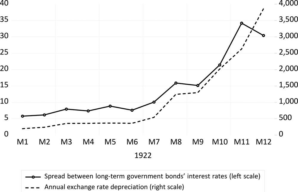
Figure 1. Spread between long-term interest rates and exchange rate depreciation
Capital outflow from Germany from July 1922 onwards bore all the hallmarks of a veritable sudden stop due to a sudden change in expectations.Footnote 8 As happens in such circumstances, the flight of capital was accompanied by a significant depreciation of the mark (Figure 1). This can be seen from the fact that the mark rose from 272 to the dollar on 1 June to 318 on 12 June, when the Morgan Report came out, and to 355 on the day of the assassination of Rathenau on 24 June. By 31 July it was at 670 and by the end of August it had reached 1,725.Footnote 9 The significant depreciation in the exchange rate that occurred in mid 1922 led to a considerable increase in both wholesale and retail prices (Figure 2).Footnote 10

Figure 2. Inflation, money supply and exchange rate depreciation
As demonstrated by Figure 2, growth in both narrowFootnote 11 and broadFootnote 12 money followed the depreciation in the exchange rate and the marked growth in prices with some delay.
As in most other cases (see, among others, Calvo and Reinhart Reference Calvo, Reinhart, Kenen and Swoboda2000; Bordo Reference Bordo, Cavallo and Meissner2007), also in Germany, the sudden stop led to a fall in output and disposable income.Footnote 13 This was followed by an exacerbation of the distributive conflict, as part of which the productive classes, workers and industrialists sought to maintain intact their purchasing power, shifting onto other interest groups the burden of diminished disposable income. The accommodating policy pursued by the Reichsbank drove this process, thus fuelling the inflationary spiral. With the acceleration of the rate of inflation output fell markedly. Consequently, between the second and the fourth quarter of 1922 the percentage of unemployed trade union workers rose from 0.6 to 2.8 per cent (see Holtfrerich Reference Holtfrerich1986, p. 198; Feldman Reference Feldman1997, pp. 603–5). The disintegration of the German economy was halted by the process of stabilisation that began in the autumn of 1923.
II
In order to corroborate the sudden stop hypothesis we carried out some causality tests. Initially we ran a VAR Granger causality test in order to make a comparison between the monetary hypothesis and the sudden stop hypothesis. To this end we considered a VAR consisting of three variables: the consumer price index, the real exchange rate of the mark with respect to the dollarFootnote 14 and the real monetary base.Footnote 15 The data are monthly and the sample period used is between January 1921 and June 1923, that is to say, the period when inflation first started to accelerate and then became explosive. As suggested by the various tests of lag length criteria, three lags have been used.
The variables used are logarithmic and expressed in first differences.Footnote 16 Before proceeding to the causality tests, Table 2 tests the hypothesis of stationarity of the variables in first differences using the ADF and the Dickey-Fuller (GLS) tests, both with the constant and with the constant and the trend.
Table 2. Unit Root Test (Jan. 1921 – June 1923; lag-length included obs. 25)

Note: The number of lags has been chosen according to the Schwarz Information Criterion.
The null hypothesis is that the variable has a unit root. ***rejected at 1%, **rejected at 5%, *rejected at 10%.
The results of these tests show that the first differences in real exchange rate (RER) and the real monetary base (RMB) are stationary. Inflation (INFL) proves to be stationary in three out of four tests.Footnote 17
After establishing the stationarity of the variables, we proceeded to the estimate of the VAR Granger causality test. The results are given in Table 3.
Table 3. Granger causality/Block exogeneity Wald test (Jan. 1921 – June 1923)
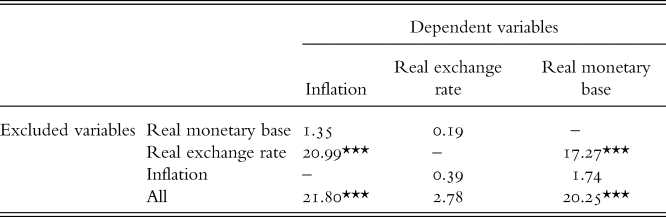
Note: Monthly change of variables. ***rejected at 1%, **rejected at 5%, *rejected at 10%.
The results in column (1) show that the null hypothesis – the interest variable does not cause inflation – is rejected in the case of the real exchange rate, while it is accepted in the case of real monetary base. As evidenced by the last column in Table 3, real exchange rate changes seem to have had notable effects not only on price growth but also on changes in real monetary base. Furthermore, neither money nor prices seem to prove significant in explaining the variation in the exchange rate.
These results acknowledge that the sudden stop hypothesis is able to explain the origin of German hyperinflation better than the monetary view. In this latter view a distinction is conventionally made between two different approaches: the monetary view in the narrow sense of the term and the monetary-fiscal view put forward by Sargent (Reference Sargent and Hall1982), which regards episodes of hyperinflation as always originating from fiscal imbalances. Conversely, according to the monetary view in the narrow sense of the term, these episodes can also result from an excessive growth in bank credit and thus from the behaviour of private individuals.Footnote 18
In order to compare the sudden stop view with Sargent's monetary-fiscal view we repeated the estimate of the VAR Granger test in Table 3, replacing the monthly variations of the monetary base in real terms (RMB) with those of government revenue in real terms (RGR).Footnote 19 The results of this test are provided in Table 3′.
Table 3′. VAR Granger causality/Block exogeneity Wald test (Jan. 1921 – June 1923)

Note: Monthly change of variables. *** rejected at 1%; ** rejected at 5%; * rejected at 10%.
These show that, as in the case of the monetary view in the narrow sense (referred to in Table 3), the null hypothesis – the variable of interest has no influence on inflation – is rejected in the case of the real exchange rate, while it is accepted in the case of real government revenue. This corroborates the sudden stop view as opposed to the monetary-fiscal view.Footnote 20
One limitation of the VAR Granger test estimated in Tables 3 and 3′ can be the shortness of the time sample under consideration. In order to test whether this shortcoming conditions the results obtained we proceeded to a robustness test of the result in Table 3 by conducting an estimate of a Bayesian VAR, in other words, an approach useful for achieving shrinkage. As Table 3′′ shows, the Block exogeneity Wald test obtained using this estimate confirms the result in Table 3: it is the real exchange rate and not the monetary base that explains inflation in the period under consideration, that is to say, between January 1921 and June 1923.Footnote 21
Table 3′′. Bayesian VAR Granger causality/Block exogeneity Wald test (Jan. 1921 – June 1923)

Note: Monthly change of variables. *** rejected at 1%; ** rejected at 5%; * rejected at 10%.
The VAR Granger test estimated in Table 3, and confirmed by the estimate in Table 3′′, provides some indications about the causal connection between the variables under consideration. It does not, however, give any indications as to the intensity of the causal links. In order to measure this intensity we used a forecast error variance decomposition (FEVD), a methodology used first by Montiel (Reference Montiel1989) and later by Dornbusch et al. (Reference Dornbusch, Sturzenegger and Wolf1990) and Fischer et al. (Reference Fischer, Sahay and Végh2002) to analyse the origin of hyperinflations. The results of the FEVD relative to the standard VAR Granger test estimated in Table 3 are given in Table 4.
Table 4. Composition of forecast error variance of variables in the VAR system (forecast at 24 months)

Panels A, B and C present three different orderings of the variables, while Panel D simply summarises the average values of the three previous orderings. Table 4 provides further evidence that the dynamics of the exchange rate significantly influence the other three variables of the system, in particular the dynamics of the rate of inflation. Conversely, the influence on this latter variable of changes in real monetary base is always lower than that of changes in the real exchange rate, irrespective of the order of the variables in the VAR.Footnote 22
It is common knowledge that in a standard VAR the result of the FEVD can be influenced by the order of the variables. A robustness test was also carried out for this estimate. We estimated a structural VAR (SVAR) which modifies the Cholesky decomposition, on which the FEVD in the standard VAR is based, in order to make the order of real exchange rate and real monetary base irrelevant.Footnote 23
It is clear from Table 4′ that in both the short and the long term the inflation dynamic is explained by shocks to the real exchange rate with percentages that are always above 50 per cent and with a slight tendency towards growth, while the contribution of the real monetary base is slightly above 30 per cent in the first six months and then falls to under 20 per cent after two years. The basic exogeneity of the real exchange rate is also confirmed. This is explained with percentages consistently slightly below 90 per cent.
Table 4′. Composition of forecast error variance of variables in the SVAR system (Jan. 1921 – June 1923)

Note: Forecast at 6, 12 and 24 months.
The results of the tests we have just described thus confirm the plausibility of the sudden stop hypothesis, namely the idea that German hyperinflation originated in an exchange rate crisis caused by a sudden stop. The next section seeks to explain when and why this sudden stop occurred.
III
It was pointed out in the Introduction that the balance of payments hypothesis assumes that German hyperinflation had its origin in an exchange rate crisis. That hypothesis maintained, however, that this crisis resulted from Germany's efforts to meet its reparations obligations. This is not the place to debate this question once again.Footnote 24 There is already a substantial literature that shows that in actual fact the effective burden of the reparations the Weimar republic had to pay was sustainable (see, among others, Schuker Reference Schuker1988; Ritschl Reference Ritschl2012).
The assumption we make here, unlike the position underlying the balance of payments hypothesis, is that the crisis of the German mark resulted from a precipitous reversal of capital flows, in other words, a sudden stop. This hypothesis makes it crucial to determine the moment when this process occurred.
An initial technique for identifying the moment when the sudden stop occurred can be the use of the SVAR historical decomposition. This approach enables us to ascertain whether the influence of variations in the real exchange rate on the rate of inflation increased over time, becoming more pronounced during the course of 1922.
In Figure 3 we give the results of this analysis across the whole period of the estimate. As can be seen, starting from the beginning of 1922, but in particular from July to December, the role of the real exchange rate in determining the variations in the inflation rate grows considerably. In particular, the phase of acceleration in inflation that occurred in mid 1922 seems to be driven primarily by the RER (Figure 3).
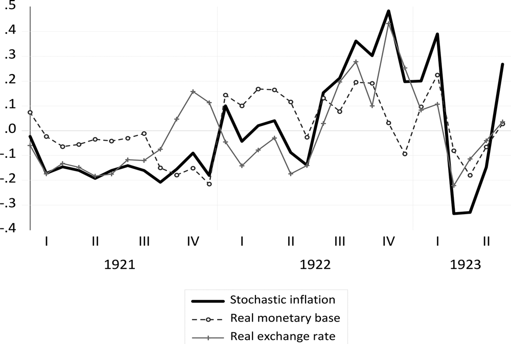
Figure 3. Historical decomposition of inflation
In order to obtain statistical confirmation of the visual impression presented by Figure 3, we regressed, by OLS, the stochastic component of inflation on the contribution of the real exchange rate and the real monetary base over three time intervals of one year, which finished in December 1921, December 1922 and June 1923, respectively. As can be seen from Figure 4, the estimates confirm the visual impression and show that the role of the exchange rate in explaining the price dynamic grew during 1922, the period when the first episodes of acceleration occurred. In particular, if the exchange rate in 1921 explains a little less than 40 per cent of the variations in prices, in 1922 it explains a little less than two-thirds of the total.
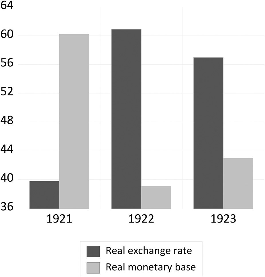
Figure 4. The relative influence of the real exchange rate and of the real monetary base on inflation
The empirical evidence outlined above shows that the influence of variations in the real exchange rate increased significantly during the course of 1922 and particularly from the latter half of the year onwards.Footnote 25
We can now try to establish which shock during this time frame led to the occurrence of a sudden stop. In order to clarify this point, we proceeded to an econometric analysis. In particular, we tested if some important pieces of political news had a significant influence on the behaviour of investors and on the exchange rate of the mark.Footnote 26
To this end we followed the ‘narrative approach’ (see Romer and Romer Reference Romer and Romer1989; Ramey Reference Ramey2011), which takes as its point of reference events recognised as important by public opinion. Following Feldman (Reference Feldman1997, p. 418), we assume that good news fuels hopes that a solution to the reparations problem will be found and the German economy will be stabilised; the opposite applies in the case of bad news. In this perspective we verify how the events listed in Table 1 influenced individual expectations and, as a consequence, the exchange rate. Since we do not have daily data for the forward exchange rate of the mark in the 1920s,Footnote 27 we attempted to determine the short-term equilibrium exchange rate using the uncovered interest parity condition.
The estimate uses the daily data of the mark–dollar exchange rate, st, the interest rate on the 3 per cent German Imperial bond, i, the interest rate on the 3.5 per cent Victory bond 1932–47, i*,Footnote 28 and the variable ‘news’, with a value of 1 for the unfavourable events and -1 for the favourable events listed in Table 1, and a value of 0 during the other periods.Footnote 29
Prior to the estimate we tested the stationarity of the variables. As emerges from Table 5, both the first difference of the exchange rate and the first difference of the spread between long-term interest rates are stationary, whichever test is used.
Table 5. Unit root tests (sample 1 Jan. 1921 – 31 Dec. 1922)

Notes: The number of lags has been chosen according to the Schwarz Information Criterion. The null hypothesis is that the variable has a unit root. ***rejected at 1%, **rejected at 5%, *rejected at 10%.
We then went on to estimate an equation specified as follows:
 $$s_t-s_{t-1} = b_0 + b_1\Delta \lpar {i_{t-1}-i_{t-1}^\ast } \rpar + b_2news_t + \varepsilon _t$$
The estimate was made by OLS for the period 1 January 1921 to 31 December 1922 and its results are shown in Table 6.
Table 6. OLS estimates of the change in the exchange rate (dependent variable st − st−1)

In column (1) we show the basic equation, where the change in the Reichsmark–US dollar exchange rate was set as a function of the change in the spread between the long-term interest rates. In the estimate this spread is significant and, as expected, positive. In column (2) we incorporated into the basic equation the variable news. Also this variable is significant and has the expected sign. In column (3) the variable news has been divided into bad news and good news. The results of the estimate show that both these variables are significant and have the expected signs. What is more, the Wald test provides no evidence of a significant statistical difference between the coefficients of the different types of news.
In order to test the robustness of the results of the estimates just described we used an extended version of the Ramey and Shapiro (Reference Ramey and Shapiro1998) approach, in particular the approach proposed by Edelberg et al. (Reference Edelberg, Eichenbaum and Fisher1998) and further refined by Romer and Romer (Reference Romer and Romer2010). As in that contribution we used a VAR with an exogenous variable: political news. Two reasons prompted the use of this type of model. Firstly, it helps overcome possible problems of endogeneity in the OLS estimates and in particular those between changes in the real exchange rate and changes in the spread. Secondly, the use of the VAR methodology makes it possible to show the impulse response function (IRF) of the exchange rate to political news.
The VAR includes the following three variables: the first difference in the mark–dollar exchange rate, the first difference in the spread between the German and the US long-term interest rates, and the variable news. In order to identify the innovations in the three variables under consideration we used the Cholesky decomposition, first ordering the variable news in the VAR system. As for the OLS estimates, the VAR system was estimated on daily data from 1 January 1921 to 31 December 1922. For each variable five lags were considered, in line with the results of the various tests of lag length criteria.Footnote 30 The VAR estimated in this way proves to be stable in that all the roots lie inside the unit circle.
The Cholesky decomposition renders the various impulses in a VAR system orthogonal by imposing order on the variables. For our purposes, having first ordered the variable news, this means that while the change in the exchange rate or in the interest rate spread reacts immediately to impulses in the variable news, this last variable reacts only with lags to shocks to the first two variables.
The estimate thus obtained enables us to evaluate the response of the exchange rate to a standard impulse of political news. Figure 5 shows the dynamic response of the change in the real exchange rate to political news over a span of ten working days.

Figure 5. Impulse response of exchange rate to political news (VAR model)
As can be seen from Figure 5, the dollar–mark exchange rate reacts significantly to political news at the moment it is announced. In the first three days it accumulates an elasticity value close to 8 per cent. Subsequently, the effects of political news on the change of the real exchange rate tend to decrease and become insignificant after the sixth day. However, because we are referring to the first difference in the real exchange rate, the increases accumulated in subsequent periods have permanent effects.Footnote 31
Since the results of the test described above may be influenced by the fact that, given that the news variable is discrete in nature, the impulse response functions obtained from the VAR can be biased and misleading, we have also computed the impulse response functions using local projections methodology. This methodology does not require specification and estimation of the unknown true multivariate dynamic system itself.Footnote 32 The estimate of the news elasticity of the real exchange rate by the local projections methodology can be found in Figure 6.

Figure 6. Impulse response of exchange rate to political news (local projection)
The news elasticity of the exchange rate, both in terms of the level and the dynamics of the impulse reflects what could be seen in Figure 5. In particular, also in this case the peak is reached on the third day up to a maximum of 7.2 per cent, after which the impulse tends to be cancelled out, becoming insignificant after the fifth day.
This evidence suggests that news, especially the news listed in Table 1, had on average important and long-lasting effects on the real exchange rate of the mark and consequently on the domestic rate of inflation.
It remains to be established whether and at what point the importance of these effects became more pronounced. To this end we consider the recursive coefficients of the estimates in Table 6. This analysis shows us that, starting from the summer of 1922, the coefficients of bad news and good news followed diverging trends (Figures 7a and 7b).

Figure 7 a. Recursive bad news coefficients b. Recursive good news coefficients
While the good news coefficient has a tendency to fall, in the case of bad news it tends to rise. This increase seems to suggest a widespread conviction that stabilisation in Germany had become unattainable. The consolidation of this conviction led to a dramatic depreciation of the mark. From late August, albeit with some delay with respect to the actual exchange rate depreciation,Footnote 33 also the three-month forward exchange rate started to show a significant discount: between the end of July and the end of August it rose from 10 to 150 per cent. Given the evidence produced we can conclude that the months between July and August 1922 represented a benchmark for expectations about Germany's economic prospects. Accordingly, Figures 7a and 7b show that from August of that year onward the influence of bad news on the exchange rate became considerably more pronounced.
This is confirmed in the estimates in column (4) in Table 6, which gives the values of the coefficients of news after 24 August 1922. A comparison of the results in this column with those in column (3) in the same table shows that after late August the bad news coefficient rose from 0.022 to 0.056, while the good news coefficient tended to lose significance.
It would seem, therefore, that starting from the end of August expectations of a growing depreciation of the mark were becoming more concrete. Confirmation of the worsening of expectations about the mark comes from the marked widening of the spread between the interest rates of German and American long-term government bonds: this grew between the middle and the end of August from 13.8 to 20.6 per cent.
Some scholars argue that the change in expectations that occurred in the summer of 1922 concerned Germany's public finances rather than the prospects of the mark. In particular, Webb (Reference Webb1986) maintains that due to the bad news of June 1922 the prospects of public finances worsened considerably. In this context, Germans expected a higher monetisation of debt and therefore a higher level of inflation. This would have prompted them to increase demand for consumer goods, thus fuelling the inflationary process. This hypothesis is consistent with the fiscal view. However, it is at odds with the evidence of the different dynamics of retail prices and wholesale prices. As shown by Table 7, in the second half of 1922, in particular from July onwards, the wholesale price index followed that of imports and the spread between wholesale and retail price indices widened markedly.
Table 7. Prices indices in second half of 1922 (June = 100)

a Workers' cost-of-living.
Sources: Bresciani-Turroni (Reference Bresciani-Turroni1937) and Holtfrerich (Reference Holtfrerich1986).
The more dynamic trend of wholesale prices compared to retail prices seems to confirm the existence of a causal link that goes from the depreciation of the exchange rate to import prices and to wholesale prices, and from these to retail prices, rather than vice versa, as Webb's (Reference Webb1986) version of the fiscal view would have it, from consumer prices to wholesale prices and from these to the exchange rate.
IV
The previous sections have shown how the origin of German hyperinflation is to be sought in a sudden stop and the consequent exchange rate crisis. However, as observed by Dornbusch (Reference Dornbusch1985), the acceleration in inflation brought about by the depreciation in the exchange rate would not have transformed into explosive inflation without an accommodating monetary policy.
The accommodating monetary policy of the central bank was in response to the worsening of the social conflict caused by the fall in output and disposable income following the sudden stop.
As in other cases of sudden stops (see, among others, Liviatan and Piterman Reference Liviatan, Piterman and Ben-Porath1986; Montiel Reference Montiel1989), the worsening of the social conflict took the form of a clash between the productive classes, workers and industrialists, on the one hand, and rentiers, on the other hand (see Kindleberger Reference Kindleberger1984a; Maier Reference Maier, Hirsch and Goldthorpe1978; Pittaluga and Seghezza Reference Pittaluga and Seghezza2012).
At a time when the country's income was falling, the unions called for real wages to be kept stable. Faced with this demand, industrialists took an accommodating attitude.Footnote 34 This attitude sprang from their concern about the possible contagion of the Bolshevik revolution and fear of union strength (see Feldman Reference Feldman, Schmukler and Marcus1983, p. 390; Holtfrerich Reference Holtfrerich, Schmukler and Marcus1983, p. 407). They therefore urged the government to adopt expansive fiscal and monetary policies so as to maintain GDP growth high and unemployment at minimum levels (see Feldman Reference Feldman1997, p. 447). Given that this was the prime goal, it is not surprising that the leading representative of the industrialists, Hugo Stinnes, argued that inflation was a ‘political necessity’.Footnote 35 In this context, a tacit alliance grew up between the industrial lobby and the workers’ unions. These two interest groups were not hostile to inflation because it enabled them to shift onto rentiers much of the fall in national income.Footnote 36
After a currency crisis generally two mechanisms can determine a further inflation rate acceleration. The first mechanism follows from the Tanzi effect, in other words, from the fact that as inflation increases, the real value of tax revenue tends to fall,Footnote 37 thus leading to fiscal deficits which, when they cannot be covered by debt, produce an excessive money supply (see Dornbusch Reference Dornbusch1985, pp. 24–5).
The second mechanism results from the fact that in phases of inflation acceleration and negative real interest rates, the demand for credit rises significantly. When this demand is satisfied, bank loans and the monetary multiplier increase (see Tullio Reference Tullio1985, p. 353). The result is a notable increase in monetary base.
In Germany in the latter half of 1922, both of these mechanisms were at work. On the one hand, mounting reductions in real government revenue began in August 1922.Footnote 38 However, the government sought to maintain a high level of spending in real terms. This implied a significant increase in fiscal deficit, in the floating debt held by the Reichsbank and in the money base created by the Treasury (Table 8).
Table 8. Government revenue, floating debt and discounted commercial bills in second half of 1922

Source: Graham (Reference GRAHAM1930).
On the other hand, in order to maintain workers’ purchasing power, re-negotiations of wages between unions and industrialists became increasingly frequent (see Colles Reference Colles1922, p. 464). As wage increases affected production costs, this inevitably led to price increases, which, in turn, had an effect on production cycles. Firms were unable to pay wages and buy capital goods, raw materials and intermediate goods using the cash flows coming from the previous period's production, since their purchasing power was eroded due to rising inflation. Especially after the sharp depreciation of the mark between 1921 and 1922, businessmen had to resort to bank credits to keep up production cycles. This helps explain why the growth of bank loans was quite considerable in 1921 and 1922 (see Prion Reference Prion1924, p. 172).
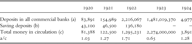
When, in mid 1922, the banks had insufficient liquidity to meet the demand for loans, the Reichsbank decided to address this situation by introducing liquidity into the system and considerably increasing the discount of commercial bills (Table 8) (see Graham Reference GRAHAM1930; Webb Reference Webb1984). Between June and December 1922 the monetary base created by refinancing operations increased by 1,416 billion in paper marks, that is to say, more than that created by the Treasury channel, which rose in the same period by 1,111 billion paper marks. At the same time, given the high level of bank loans, the significant growth of the monetary base was accompanied, between 1920 and 1922, by a particularly sharp increase in the money multiplier (Table 9).

The acceleration of the inflation rate eroded the real value of the public debt in the national currency. This erosion inflicted significant capital losses on rentiers, the principal holders of government bonds.
V
In the years following the Treaty of Versailles, Germany benefited from a massive inflow of capital from abroad. This influx was driven by expectations of an appreciation of the Reichsmark. Foreign investors were confident that the reparations problem would be resolved and that the German economy would be stabilised. However, in the summer of 1922, in the wake of some bad events foreign and domestic investors lost confidence in the future appreciation of the German currency. This change in expectations was followed by a sudden stop. The reversal of flows of capital led to a significant depreciation of the mark, an accelerating rate of inflation and a fall in output and disposable income.
As is often the case in emerging countries hit by a sudden stop, also the German government was unable to adopt policy measures designed to offset its consequences. Opposition to these measures came primarily from labour and industry. In particular, the unions demanded that workers’ purchasing power be kept stable. These demands were accepted by industrialists because they were convinced that any possible rejection would lead to unrest and potentially to a revolutionary coup similar to the Bolshevik uprising in Russia. This condition could only be met through a continuous depreciation of the mark and a significant increase in the exposure of companies to debt. In this way, they received loans from banks to pay workers and to buy intermediate goods, and repaid them with money that had lost value due to a fall in the exchange rate.
Income support for the productive classes by means of the measures outlined above took the form of a broad-based redistribution process at the expense of other social classes, notably rentiers (see Morelli and Seghezza Reference Morelli and Seghezza2014).
Supplementary materials and methods
To view supplementary material for this article, please visit https://doi.org/10.1017/S0968565020000062


 Open access