The Social Justice Impact of the Transit-Oriented Development

Abstract

Transit-oriented development (TOD) is often considered a solution for automobile dependency in the pursuit of sustainability. Although TOD has shown various benefits as sustainable development and smart growth, there are potential downsides, such as transit-induced gentrification (TIG). Even if there were no displacement issues with TIG, existing residents could be disadvantaged by a TOD due to affordability problems. This study focuses on these potential affordability issues and aims to evaluate the effects of TOD using residents’ discretionary income (DI) as an indicator of affordability. The light rail transit-oriented development (LRTOD) in Phoenix, AZ, is selected because of the timing of the introduction of development and the simplicity of the light rail transit line. In order to counteract problems induced by a non-random location of TODS, propensity score matching is used. The results indicate that LRTOD can give benefit to all TOD residents. Moreover, the effects of LRTOD on discretionary income of various types of households are not statistically significantly different. We have identified the different magnitudes of the effects of TOD between propensity score matching (PSM)-controlled and uncontrolled models. These indicate the existence of the selection bias of TOD implementation, justifying the adoption of the PSM method.

1. Introduction

Transit-oriented development (TOD) is often considered a solution for automobile dependency in the pursuit of sustainability. TOD is a form of comprehensive economic transit infrastructure development, combining transit infrastructure with a pedestrian-friendly environment and mixed land-use [1,2,3,4]. Although TOD has shown various benefits in sustainable development and smart growth, there may be potential downsides, such as transit-induced gentrification. That is, the benefits from TOD, such as improved accessibility, walkability, and environment, could be capitalized into land values, which thus increases housing prices and rent [5,6,7,8]. If the increases in residential costs outrun the benefits of TOD, such as an increase in incomes due to the revitalization and/or decrease in transportation costs, transit-induced gentrification can result. There have been arguments that transit-induced gentrification (TIG) can accompany and/or trigger displacement of minorities and lower-income families [8,9,10]. Even if there turns out to be no displacement with TIG, TOD can disadvantage existing residents due to affordability problems [6,11,12]. It is imperative for policymakers and practitioners to understand how a TOD project affects the residents in terms of affordability. Moreover, the lower-income household, such as a poor renter, used to be disregarded [13].

This study, therefore, utilizes the concept of discretionary income, which can apprehend affordability and the phenomena of gentrification, i.e., change in incomes and indispensable expenditures. The indispensable expenditures are defined as residential costs and transportation costs which are based on the Location Affordability Index data.

This study aims to evaluate the effects of TOD on residents’ discretionary income (DI) by estimating the differences in DI between TOD and non-TOD areas across various types of households. The light rail transit-oriented development (LRTOD) in Phoenix, AZ, is selected as the study area because of the timing of the introduction of development and the simplicity of the light rail transit line. Propensity score matching (PSM) is used to correct for bias due to non-random assignment of TODs to neighborhoods (TODs tend to be placed in lower-income neighborhoods). The results indicate that LRTODs can benefit all TOD residents because DIs in TOD neighborhoods are greater than in non-TOD neighborhoods. Moreover, the effects of LRTOD on the DIs of various types of households within TOD areas are not statistically significantly different. We have identified the different magnitudes of the effects of TOD between PSM-controlled and uncontrolled models. These indicate the existence of the selection bias of TOD implementation, justifying the adoption of the PSM method.

The rest of this paper is arranged as follows: Section 2 is the theoretical background of TOD, TIG, and DI. Section 3 describes the research framework, including data and methodology. Section 4 provides and interprets the results. Section 5 concludes.

2. Theoretical Background

2.1. Transit-Oriented Development and Gentrification

Transit-oriented development (TOD), as sustainable or equitable development, is taking the lead in practice and theory. A TOD is a form of comprehensive economic transit infrastructure development, incorporating transit infrastructure with a pedestrian-friendly environment and mixed-land use. A TOD can “increase accessibility to employment, educational, cultural, and other opportunities by promoting transportation options to households, thereby increasing transit ridership and reducing road congestion” [1] (p. 5). A TOD is believed to have many benefits: halting incessant sprawl, increasing ridership so as to reduce congestion, revitalizing old neighborhoods, providing economic returns to surrounding landowners and businesses, and improving safety for nonmotorized infrastructure [1,3,4,6,14,15,16,17,18,19,20,21,22,23]. Although there are many benefits of transit-oriented development (TOD), transit-induced gentrification (TIG) is a concern. However, the association between TIG and the implementation of light rail transit-oriented development (LRTOD) is unclear. In theory, gentrification can trigger population displacement because improved accessibility, walkability, and the environment are capitalized into land values, which thus increases housing prices and rent [5,6,7,8]. Consequently, lower-income households may relocate because housing has become unaffordable, and even if they stay, they may be excluded from the benefits of TOD because increases in residential costs cancel out the benefits of accessibility, i.e., transit-induced gentrification [8,9,10].

This study specifically splits gentrification into two categories, although most studies consider gentrification as a single concept. Here, the term “residential gentrification” is used to refer to the phenomena on that the capitalization of better accessibilities and environments into land and housing values increases residential costs [8,9,10]. “Commercial gentrification” refers to the fact that local and inexpensive commerce is often displaced as a result of rising rents. This is not dealt with in this study. Rather, this study mainly focuses on the phenomenon of residential gentrification caused by transit-oriented development, which we refer to transit-induced gentrification (TIG).

The concern about TIG is the core motivation. Implementation of a TOD can improve accessibilities via better environments and reduce transportation costs. However, those improved accessibilities can be capitalized into land values, thus raising costs such as housing rents. When residential gentrification happens, residents typically have two choices: (1) residents who cannot afford rising costs move out from their neighborhoods; (2) they decide to accept the higher rent because they are able to get a better paying job than before, or they can reduce transportation expenditures to offset higher residential costs [24]. There are many studies regarding the relationship between TIG and the displacement of low-income residents. Scholars still debate whether TOD can trigger these problems [6,11,12]. Nonetheless, whether or not displacement happens, low-income residents can still be worse off if rents increase, while the other costs, such as transportation costs do not decrease enough to compensate for this difference, holding incomes constant [25]. Moreover, in public decision-making processes and developments, poor renters may be disregarded, while focusing on the benefit of developers and homeowners in TOD areas [26,27].

On the other hand, TOD supporters have suggested that transit-induced gentrification will not occur because transportation costs will decline, and incomes increase because of TOD’s features [3,14,15,18,23,28,29,30]. The premise of this argument is that the changes in transport expenditures and income can “net out” rising residential costs sufficiently and prevent displacement. Many researchers have attempted to identify the effects of TOD on each expenditure or on income, as well as their proportion, e.g., location affordability. However, there is insufficient evidence to support the proposition that an increase in income combined with a decrease in transport expenditures will exceed the increase in residential costs. Moreover, the amount of “net out” can vary across types of households, from middle-income to lower-income. For example, lower-income households may receive fewer advantages or more disadvantages from TOD than middle-income households do.

2.2. Discretionary Income and Transit-Induced Gentrification

TOD may be able to enhance job accessibility so as to raise household income. Household income explains consumption behaviors and patterns. The premise is that earning more and spending more shows that one is better off, although family income is not always a good indicator [31]. Regarding transit-induced gentrification (TIG), a family in a TOD area might earn more but have to spend more on essentials such as rent compared with a family in a non-TOD area, ceteris paribus. Then, it is not clear, as simply comparing incomes cannot show whether a TOD is beneficial to the household’s economic situation. However, if the family income after indispensable costs, e.g., residential and transportation costs, in the TOD area is higher than for those in the non-TOD area, then living in the TOD area can be regarded as beneficial. Therefore, this paper focuses on income after indispensable costs, what we refer to as discretionary income (DI).

Spending power can depend on DI [24,31,32]. There are various types of DI, e.g., subjective and objective. Regardless, the crux of DI is how much money a consumer unit can spend on nonessentials. In this study, DI is defined as income after transportation and residential costs. That is, transportation and residential costs are the only necessities considered. O’Guinn and Wells [31] reviewed the previous literature on subjective discretionary income (SDI), i.e., the amount of discretionary income a family subjectively believes to have. The authors stated that the SDI could be “informative”, i.e., showing subjective life satisfaction and economic well-being. Thus, this study assumes that DI reflects economic well-being, i.e., the benefit of TOD, which can cause gentrification (increases in rent) and enhance accessibility (a decrease in transportation cost), thus possibly job accessibility (an increase in household income). These changes will net out in changes in DI. This study, thus, assesses the extent of advantages or disadvantages a TOD can render regarding economic well-being by taking DI into account.

2.3. Selection Bias in Implementation of Transit-Oriented Development

TOD has various objectives: Enhance transit accessibility and walkability, provide open space, and offer mixed land use and inclusionary zoning [1,3,27,29,33,34,35,36]. In addition, TOD is implemented with the intention to revitalize disinvested areas, which can be either urban or suburban. Calthorpe [37] categorized the types of TOD neighborhoods as residential neighborhoods and urban areas. Dittmar and Poticha [38] defined the typology of TOD locations as downtown, urban neighborhoods, suburban town centers and neighborhoods, neighborhood transit zones, and commuter towns.

As previously mentioned, this study focuses on the TOD in Phoenix, AZ. This implementation is located in the downtown area (Central Business District, CBD. Phoenix, Arizona). TOD station areas in the pre-development period (2000) were composed of employment and amenity centers and impoverished urban areas. Most of the employment and amenity centers were made up of offices and services, and only 10% was residential land. Meanwhile, the surrounding impoverished urban areas were characterized as those with the lowest household incomes (USD 19,202, [39]). This implies systematic differences in characteristics between TOD and non-TOD neighborhoods at the pre-development period. This heterogeneity can hamper an accurate estimate of the effect of a TOD on the DI across different types of households. For example, we can assume that impoverished neighborhoods have a greater difference in DIs between low- and middle-income households than other areas in the pre-development period. Even though a TOD could help raise DI of low-income households relative to middle-income households, the difference in DIs between these households in the TOD area can be smaller than that in the non-TOD area because of the pre-existing gap of DIs. This can lead a study to incorrectly conclude that there is a negative impact of TOD on low-income households over middle-income households, as DI data are available only in the post-treatment period (i.e., after the establishment of a TOD). Therefore, eliminating sample selection bias in the neighborhood in which a TOD is implemented is important if this study intends to find the true effect of TOD.

2.4. TOD’s Effect on Indispensable Expenditures

Because there is little research on the relation between TOD and overall DI, this section reviews the association between TOD and DI’s components, i.e., transportation and residential costs. According to the Consumer Expenditure Survey, housing and transportation costs are the first and second greatest household expenditures, and scholars have addressed their importance in housing affordability [24,40,41,42,43].

Renne and Ewing [14] compared TOD neighborhoods with other transit neighborhoods and found that TOD residents spend less on housing and transportation. Renne, Tolford, Hamidi, and Ewing (2016) [30] extended Renne and Ewing’s work [14] and examined the residential and transportation costs in transit neighborhoods in the US. They categorized the stations and neighborhoods as TOD, transit adjacent (TAD), and Hybrid based on walkability and land-use. They found that the residential costs in TOD areas were higher than in the other areas; however, lower transportation costs offset the higher residential costs. As a result, they concluded that TOD neighborhoods are more affordable than other areas (TAD and Hybrid). However, this study compared only station areas, which cannot be used to evaluate TOD’s effects overall [24], because TOD is the combination of transit service, land use planning, and environmental design. Bardaka et al. [44] investigated the spillover effects of transit-induced gentrification in Denver’s light rail neighborhoods. They defined transit-induced gentrification as changes in the median household income, educational attainment, managerial occupation, and housing value. They found that after TOD was implemented in rundown neighborhoods, gentrification tended to follow, which led to increased income, housing values, and so forth. Bartholomew and Ewing [45] reviewed the literature on the relation between hedonic price and TOD. They found that most of the literature has indicated that high demands for a pedestrian-friendly environment with transit services are capitalized into the land’s value and real estate prices. This implies that TOD can increase residential costs, and thus, it could play a prominent role in the real estate market and economy. Meanwhile, Dong [46] stated that TOD does not make rent or homes unaffordable. The author also found no statistically significant evidence of gentrification in TOD in the Portland, OR metropolitan areas.

Recently, Baker and Kim [24] addressed the effect of light rail transit on DI in the US and calculated DIs for 2000 and 2010 using complex systems of equations. Average transportation and residential costs were regressed using various predictors, and based on average household income in a census block group derived from census data. Finally, they compared the change in DI between light rail transit neighborhoods and other areas. They concluded that the average DI decreased less in light rail transit neighborhoods compared to other areas except in Los Angeles and Seattle. However, this study did not take into account the impact on various types of households, e.g., lower-income or middle-income households. Moreover, they did not distinguish LRTOD from light rail transit.

2.5. Research Gap and Research Question

The previous literature shows that the introduction of a TOD may decrease transportation costs and increase residential costs as well as income. However, the evidence for these effects is not conclusive. Although a recent study [24] showed the way light rail transit affected DI which can consider the phenomena of TIG and the quality of life, it did not shed light on how equitably TOD affects DI across various types of households. Moreover, the systematic differences between TOD neighborhoods must be considered to assess TOD’s unbiased effects.

This study is designed to fill several gaps. First, a conditional difference-in-difference approach is used to make an unbiased comparison. Second, DI is used to evaluate the effects of LRTOD. Finally, in the context of social justice, because LRTOD can confer its dis/advantages unequally, the TOD’s benefits on various types of households’ income levels are compared. Accordingly, this study answers the following questions:

•

Is DI lower or higher in an LRTOD area than a comparable area without LRTOD?

•

Is the difference in DI following the introduction of LRTOD greater for a lower-income household than for a middle-income household?

•

How does the systematic difference in the implementation of TODs affect estimating its impact on DI?

3. Research Framework

3.1. Data

As light-rail transit-oriented development (LRTOD) is a prevalent form of TOD in the United States [14,29], this study focuses on a single case of LRTOD: Phoenix, Arizona. The light rail transit in Phoenix has only a single line, thereby obviating the need to consider complex network effects. The initial light rail system was opened on 27 December 2008, and had 28 stations. No stations were opened thereafter until 2013. Because the LAI was developed using the American Community Survey between 2008 and 2012, and because there was no intervention or change in the light rail system during that period, Phoenix is an appropriate area to isolate the light rail system’s effects.

This study uses the Location Affordability Index (LAI) data (version 21). DI in this study is defined as income after non-discretionary spending (transportation and residential costs). The LAI dataset provides income and costs across different types of households. (

Table 1. Type of households in the Location Affordability Index (LAI).

Household Profile	Income Ratio to the Median Household Income (MHHI) for a Given CBSA2	Household Size	Number of Commuters
Median-Income Family	100% of MHHI	4	2
Very Low-Income Individual	National poverty line	1	1
Working Individual	50% of MHHI	1	1
Single Professional	135% of MHHI	1	1
Retired Couple	80% of MHHI	2	0
Single-Parent Family	50% of MHHI	3	1
Moderate-Income Family	80% of MHHI	3	1
Dual-Professional Family	150% of MHHI	4	2

) As this study is designed to understand the way LRTOD can affect different levels of household income, its effects on eight household profiles are investigated. Thus, this study uses transportation, residential costs, and household income for the eight types of households.

Table 2. List of variables.

Variable	Description	Source
Expenditure
Discretionary Income	Household Income—Transportation Cost—Residential Cost for each type of households	LAI
Household Income	A household income for each type of households	LAI
Transportation Cost	A transportation cost for each type of households	LAI
Residential Cost of SP	A residential cost for each type of households	LAI
Neighborhood Characteristics
TOD neighborhood	1 if a census block group is a TOD neighborhood, otherwise 0	Renne and Ewing (2013)
Total population (2000)	Total population in a census block group in 2000	Census
Commuting Worker (2000, %)	A percentage of commuting worker to total population	Census
Median year of building (2000)	Median year of the buildings built in a census block group in 2000	Census
Urban or Suburban (2000)	A binary variable. 1 if a census block group is an urban area in 2000, otherwise 0.	Census
Poverty ratio (2000)	Population for whom poverty status is determined/total population in 2000	Census
Race: White (2000, %)	A percentage of White population in a census block group in 2000	Census
Urban population (2000, %)	A percentage of urban population in a census block group in 2000	Census

represents the list of variables for this study. The descriptive statistics are represented in Appendix A

The geographical unit of this study is the census block group. Renne and Ewing (2013) evaluated the transit neighborhoods and provided a list of the TOD stations that opened between 2000 and 2010, and categorized them as TOD, TAD, and HYBRID stations3. I consider TOD stations as the stations alone, and exclude the other stations. I use the following criteria to assign TOD neighborhoods to a census block group: (1) The station is in a census block group; or, (2) a one-mile buffer from a station overlaps 25% of a census block group, or (3) a block group’s centroid is within one-mile of a station.

3.2. Methodology

3.2.1. Difference-in-Difference Regression

This study is designed to compare the advantages/disadvantages of TODs between lower-income and middle-income households (across all levels and types of households). The initial step in the research is to compare the DI between TOD and non-TOD neighborhoods directly. To do this, we employ a difference-in-difference (DiD) regression:

$$Y_{ih}= \alpha + \beta \times X_i+ \rho T_i+\gamma H_h+ {\delta }_h\left(T_i\times H_h\right)+ {\epsilon }_{ih}$$

(1)

where $Y_{ih}$ is the DI of household type $h$ in census block group $i$; $\alpha$ is an intercept that indicates the grand mean of the DI; $X_i$ is a vector of neighborhood characteristics; $T_i$ is a binary variable that indicates whether a neighborhood is a TOD neighborhood ($T_i=1$) or not ($T_i=0$), and $H_h$ is a categorical variable that represents the household types in Table 1. In Equation (1), the estimator ${\delta }_h$ is the DI advantage of the TOD for household type, $h$ compared to the median income household. Note that, unlike the other traditional DiD methodology, this analysis lacks the pre-treatment period data. Instead, the treatment and control groups have subgroups by income level and types of households. Thus, the first difference of the DiD of this study is the difference of DI between treatment and control group and the second difference is the difference of DI between subgroups.

3.2.2. Selection Bias in TOD’s Location

However, TODs are not assigned randomly in neighborhoods, which can lead to a selection bias in estimating the effects of TOD. To correct for this, propensity score matching (PSM) is used to eliminate the selection bias.

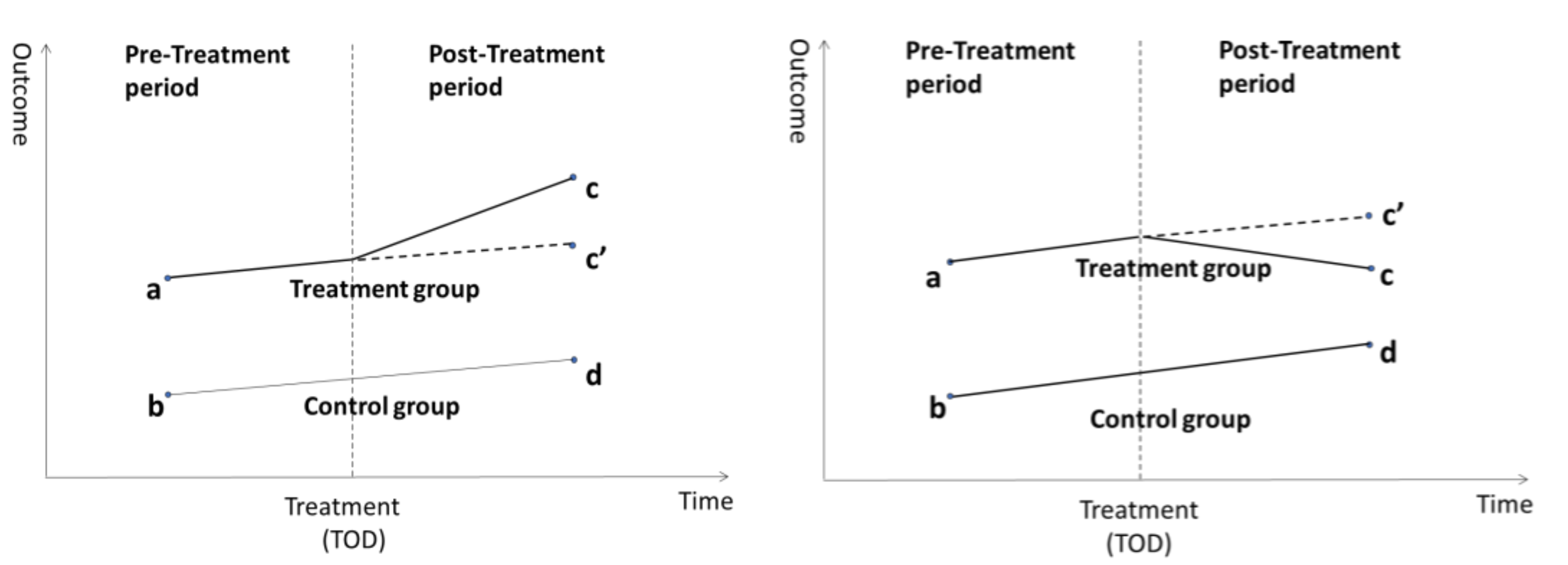
This is explained in Figure 1, where the treatment group is TOD neighborhoods, and the control group is non-TOD neighborhoods. The difference in outcomes (DI) before the treatment (TOD implementation) is $\overline{ab} (\ne 0$), which implies that the treatment and control neighborhoods differ systematically with respect to the outcomes (the treatment assignment is non-random). Both sides of Figure 1 show that during the post-treatment period, the treatment group ($c$) outcomes are greater than those of the control group (d). If we saw the outcomes only during the post-treatment period (i.e., c and d), we would conclude that TOD is associated positively with the outcome for both cases in Figure 1. However, once the outcomes in the pre-treatment period are shown, we can distinguish two cases: the TOD can increase the outcome by the amount of $\overline{c^{\prime }c}$in the left case, while it can reduce the outcome by the difference between $c^{\prime }$ and $c$ in the right case. Thus, in the ideal setting, because the pre-treatment period data are available, it is unnecessary to be concerned with non-random assignment of the TOD’s implementation.

Conversely, non-random assignment of TOD can be a source of bias. Referring to Figure 1 again, assuming that TOD is not assigned randomly, the outcomes in the post-treatment period show that the outcomes in the treatment neighborhood are greater than those in the control neighborhood. However, without the pre-treatment information on the outcomes (a and b), we cannot discover TOD’s effect on the outcomes, i.e., we cannot tell whether $\overline{ab}$ was greater or smaller than $\overline{cd}$.

However, as shown in Figure 2, using a conditioning method, such as propensity score matching, to select “similar” neighborhoods (i.e., where $a=b$, pre-treatment) can eliminate the systematic difference $\overline{ab}$. Hence, an unbiased estimate of TOD’s effects on the outcomes is $\overline{cd}= \overline{c^{\prime }d}$. Figure 2 shows that, when neighborhoods are controlled, we can determine the unbiased effects of TOD. Thus, corresponding to the available information and research question, this study employs a PSM estimator to correct for the TOD-assignment bias. Note that the critical assumption of this analytical framework is to identify the “similar” controlled neighborhood based on the explanatory variables in a conditioning method, such as propensity score matching.

3.2.3. Conditional Difference-in-Difference with Propensity Score Matching

The estimator ${\delta }_h$ in Equation (1) can be biased because the decision to implement a TOD is non-random (selection bias). To eliminate this bias, and to proceed as if the assignment of TODs to neighborhoods was random, this study uses propensity score matching (PSM). PSM allows any selection bias to be eliminated, and the treatment (TOD) to be considered as if assigned conditionally at random [47,48,49,50,51].

A balancing score $s\left(x\right)$ is a function of covariates x, which are associated with TOD implementation. Thus, the conditional distribution of $x$ given $s\left(x\right)$ is the same for TOD and non-TOD neighborhoods. This implies:

$$x\perp T | s\left(x\right)$$

(2)

In principle, $s\left(x\right)$ can be any functional form, but in PSM, $s\left(x\right)$ is the probability that a neighborhood is selected for TOD

$$P_i=\mathrm{Pr}(T_i=1 |X_i^{\prime }) = s\left[L\left(X_i^{\prime }\right)\right]$$

(3)

which we estimate by logit regression. The logit regression’s observed variable is $T_i$. $X_i^{\prime }$ is a vector of covariates, which in this case consists of neighborhood characteristics associated with TOD implementation. $L\left(\cdot \right)$ is a linear function, and $s\left(\cdot \right)$ is the logistic function. The TOD and non-TOD neighborhoods are selected on the basis of similar estimated propensity scores. Thus, there is no significant systemic difference between TOD and non-TOD neighborhoods with respect to the covariates used in the logistic regression. In this study, we use Matchit package [52] in R. Non-TOD neighborhoods are selected 5 times to the TOD neighborhoods while the detailed PSM algorithm is in Appendix B.

As PSM solves the problem of sample selection bias for TOD implementation, DiD can mitigate the endogeneity problem attributable to omitted variables bias, and the PSM-DiD approach (Equation (4)) can estimate the TOD’s effect on the DI accurately [53]:

$$Y_{ih}= {\alpha }^{\prime }+ {\beta }^{\prime }\times X_i+ {\rho }^{\prime }{\widehat{T}}_i+{{\gamma }^{\prime }}_h{H}_h+ {{\delta }^{\prime }}_h\left(T_i\times H_h\right)+{\epsilon }_{ih}^{\prime }$$

(4)

where $i$ ranges over the PSM-matched neighborhoods. Thus, ${\widehat{T}}_i$ indicates PSM-selected TOD and non-TOD neighborhood: TOD neighborhood ($T_i=1$) or not ($T_i=0$). In summary, the coefficients of the regression (4) can answer the research questions: ${\rho }^{\prime }$ can represent whether DI in a TOD neighborhood is greater or less than that in a non-TOD neighborhood. In addition, ${{\gamma }^{\prime }}_h$ shows the way DI differs between the household types, $h$. Finally, the estimator ${{\delta }^{\prime }}_h$ can show the DI advantage of TOD for each type of household compared to the base type of household, e.g., Median Income Family. For example, if ${{\delta }^{\prime }}_h$ is significantly negative, a household $h$ is disadvantaged in a TOD neighborhood compared to a Median Income Family.

4. Results

4.1. Control Neighborhood Selection Using Propensity Score Matching

This study categorized the TOD stations’ neighborhoods, according to Renne and Ewing’s work. Then, TOD and non-TOD neighborhoods’ DI were compared. As discussed earlier, however, TOD was not implemented randomly, which means that the characteristics of TOD and non-TOD neighborhoods may differ, and this affects the evaluation of the TOD’s influence (selection bias). Therefore, PSM was performed to identify the control non-TOD neighborhood identical to the TOD neighborhood. This section explains why PSM solves the problems and shows how the PSM algorithm chooses the “similar” non-TOD neighborhoods as a control group. The detailed outcomes of PSM are in Appendix A.

The neighborhood characteristics of TOD and non-TOD neighborhoods in 2000 were compared using census data. (

Table 3. Comparison of transit-oriented development (TOD) and Non-TOD neighborhoods.

Variable	Means of All Data		Means of Matched Data
	TOD	Non-TOD	TOD	Non-TOD
Total population (2000)	1400.4	1397.747	1400.4	1523.573
Population density (2000)	0.002	0.002	0.002	0.002
Race: White (2000, %)	0.624	0.769	0.624	0.666
Median year of building (2000)	46.7	20.768	46.7	39.153
Poverty ratio (2000)	0.359	0.118	0.359	0.233
Commuting Worker (2000, %)	0.334	0.46	0.334	0.365
Urban population (2000, %)	1	0.968	1	1

) The two left columns show the averages for all study areas, while the last two show averages after PSM-matching. The table shows that the characteristics of the non-TOD neighborhoods were similar to those of TOD neighborhoods after matching except for the total population. For example, the mean proportion of Whites in the population in non-TOD areas was significantly higher than in TOD areas before they were PSM-controlled (76.9% and 62.4%, respectively). After PSM, the mean proportion of Whites in the non-TOD areas decreased to 66.6%, and thus, there is only a 4.2% difference from that in TOD areas. (Figure 3)

Figure 4 shows that, geographically, the areas chosen as non-TOD control neighborhoods are located near TOD neighborhoods, although some areas are located on the east and north sides of urban areas. Regardless, the control areas appear to be located in the same metropolitan areas, and thus are comparable.

4.2. Discretionary Income Model Outcomes

The outcomes of the DI models are presented in

Table 4. Discretionary income models.

	Dependent Variable: Discretionary Income
	Using All Areas				Using PSM-Matched Areas
	(1)	(2)	(3)	(4)	(5)	(6)	(7)	(8)
TOD neighborhood	4041.32 ***		4041.32 ***	4217.62 ***	2555.65 *		2555.65 ***	2815.61 ***
	(1240.43)		(334.85)	(947.30)	(1336.38)		(252.50)	(715.53)
Very Low-Income Individual		−30,529.40 ***	−30,529.40 ***	−30,513.40 ***		−30,625.70 ***	−30,625.70 ***	−30,517.80 ***
		(209.14)	(207.60)	(210.25)		(389.51)	(376.41)	(413.11)
Working Individual		−17,176.70 ***	−17,176.70 ***	−17,154.70 ***		−17,389.10 ***	−17,389.10 ***	−17,257.60 ***
		(209.14)	(207.60)	(210.25)		(389.51)	(376.41)	(413.11)
Single Professional		22,954.00 ***	22,954.00 ***	22,950.20 ***		23,303.40 ***	23,303.40 ***	23,343.90 ***
		(209.14)	(207.60)	(210.25)		(389.51)	(376.41)	(413.11)
Retired Couple		−3891.48 ***	−3891.48 ***	−3887.30 ***		−4008.52 ***	−4008.52 ***	−3998.80 ***
		(209.14)	(207.60)	(210.25)		(389.51)	(376.41)	(413.11)
Single-Parent Family		−20,583.00 ***	−20,583.00 ***	−20,567.80 ***		−20,840.50 ***	−20,840.50 ***	−20,772.10 ***
		(209.14)	(207.60)	(210.25)		(389.51)	(376.41)	(413.11)
Moderate-Income Family		−7481.73 ***	−7481.73 ***	−7476.35 ***		−7543.22 ***	−7,543.22 ***	−7512.90 ***
		(209.14)	(207.60)	(210.25)		(389.51)	(376.41)	(413.11)
Dual-Professional Family		23,643.70 ***	23,643.70 ***	23,619.50 ***		24,396.50 ***	24,396.50 ***	24,354.70 ***
		(209.14)	(207.60)	(210.25)		(389.51)	(376.41)	(413.11)
Very Low-Income Individual $\times$ TOD				−651.60				−647.17
				(1339.68)				(1011.92)
Working Individual $\times$ TOD				−891.94				−789.05
				(1339.68)				(1011.92)
Single Professional $\times$ TOD				150.40				−243.28
				(1339.68)				(1011.92)
Retired Couple $\times$ TOD				−169.79				−58.29
				(1339.68)				(1011.92)
Single-Parent Family $\times$ TOD				−614.95				−410.70
				(1339.68)				(1011.92)
Moderate-Income Family $\times$ TOD				−218.50				−181.96
				(1339.68)				(1011.92)
Dual-Professional Family $\times$ TOD				986.00				250.79
				(1339.68)				(1011.92)
Constant	21,353.30 ***	25,586.00 ***	25,486.40 ***	25,482.10 ***	22,839.00 ***	27,353.40 ***	26,927.40 ***	26,884.10 ***
	(194.67)	(147.88)	(147.03)	(148.67)	(545.58)	(275.43)	(269.47)	(292.12)
Observations	9744	9744	9744	9744	1440	1440	1440	1440
R2	0.001	0.93	0.93	0.93	0.003	0.96	0.96	0.96
Adjusted R2	0.001	0.93	0.93	0.93	0.002	0.96	0.96	0.96
Residual SE	18,978.60 (df = 9742)	5161.06 (df = 9736)	5123.14 (df = 9735)	5124.27 (df = 9728)	18,899.30 (df = 1438)	3695.25 (df = 1432)	3570.94 (df = 1431)	3577.67 (df = 1424)
F Statistic	10.61 *** (df = 1; 9742)	17,448.70 *** (df = 7; 9736)	15,512.70 *** (df = 8; 9735)	8269.97 *** (df = 15; 9728)	3.66 * (df = 1; 1438)	5182.68 *** (df = 7; 1432)	4868.89 *** (df = 8; 1431)	2587.08 *** (df = 15; 1424)

Note: *p < 0.1; *** p < 0.01.

. The first four columns (1)~(4) are the outcomes of the model that uses all of the study areas based on Equation (1), while the other models are estimated based on the PSM-controlled areas.

Firstly, all models indicate consistently that DIs in TOD neighborhoods are greater than them in non-TOD neighborhoods, as all coefficients of TOD neighborhood are positive throughout all models. This implies that a TOD has a positive effect on DI overall. Further, TOD helps enhance the household’s economic situation on average for all types of households. These outcomes lend a meaningful policy implication to the TOD planner and policymakers. That is, TOD may be able to prevent transit-induced gentrification. For example, a recent study [24] addressed that light rail transit in Pheonix may decrease DI since DIs of light rail neighborhoods (LRN) decreased compared to those in non-light rail neighborhoods (non-LRN). However, this study shows that TOD principles can make a difference because the DIs in TOD neighborhoods (parallel to the LRN in the study [24]) are greater than the DIs in non-TOD neighborhoods (parallel to the non-LRN in the study [24]). This implies that the transit neighborhoods with TOD principles, such as better accessibility, environmental quality, and mixed land use, can better off the households regarding DI while the transit neighborhoods without TOD principles may not.

Regardless of the consistent directions of the estimates’ signs, their magnitudes varied. For example, when the first four models are compared with the others, which can represent the effect of selection bias of TOD implementation, the coefficient of TOD neighborhood in column (3) is greater than that in column (7), i.e., 4041.32 and 2555.65, respectively. This indicates that the extent of the TOD’s effect decreases because of eliminating selection bias in TOD implementation, suggesting that the DI of the neighborhoods where TOD is likely to be introduced is higher than that of the other neighborhoods. This may justify using conditioning algorithms in order to find comparable control neighborhoods. Since the TOD neighborhoods in Pheonix were characterized as impoverished areas with higher poverty ratio and a lower portion of commuting workers at the pre-TOD period, PSM, as a conditioning algorithm, finds similar neighborhoods at the same period. The decreased size of the coefficient of TOD neighborhood also suggests that effects of TOD could have been overestimated if the reference group is not appropriately dealt with.

The models in columns (4) and (8) indicate that, contrary to expectations, the differences in the TOD’s effects are statistically insignificant across all types of households. This may be because TOD can be beneficial to an entire population’s DI, which is unlikely to be the case with household income, or without TOD stations. For example, Pollack et al. [36] addressed the concerns of adverse effects of gentrification in transit-rich neighborhoods, which is a housing cost burden for low-income residents. It suggests an implicit policy implication that the introduction of TOD can affect social equity, e.g., winners and losers in transportation policy [13,36,54,55,56]. Thus, Pollack et al. [36] stressed TOD’s principles in “A Toolkit for Equitable Neighborhood change in Transit-Rich Neighborhoods.” At least, the TOD in Phoenix seems to be successfully implemented as the TOD was introduced without changing the economic equality in the TOD neighborhoods compared to the non-TOD neighborhoods.

Additionally, the DIs vary across types of households. For example, in column (2), the comparative magnitudes of DIs are in line with the household income defined by LAI (

Table 5. Comparing rank between discretionary income (DI) and household income across types of household.

Household Profile	Income Ratio to the Median Household Income (MHHI) for a Given CBSA	The Rank of Discretionary Income Based on Model (6)
Dual-Professional Family	150% of MHHI	1
Single Professional	135% of MHHI	2
Median-Income Family	MHHI	3
Retired Couple	80% of MHHI	4
Moderate-Income Family	80% of MHHI	5
Working Individual	50% of MHHI	6
Single-Parent Family	50% of MHHI	7
Very Low-Income Individual	National poverty line	8

). The smaller rank means the higher DI. It shows that a family with a higher income has a higher DI. Interestingly, Retired Couple and Moderate-Income family have the same level of household income, but the Moderate-Income family has lower DI. This is probably because the costs of the Moderate-Income family exceed those of the Retired Couple due to the number of commuters and household size. That is, the greater numbers of commuters and the household size mean the higher transportation cost and residential cost (i.e., larger house), respectively. Likewise, the DI of Working Individual is greater than that of Single-Parent family.

A possible limitation of this result is the way the LAI data are constructed. The LAI was derived by structural equation modeling (SEM) using sociodemographic information. The process of SEM might be able to eliminate the possible errors/effects that could manifest as the effects of the interaction terms, e.g., the heterogeneities in TOD’s influence across types of households. This also can be the reason the predictive power ($R^2$) is very high. Moreover, the DI is calculated by fixing the household income based on the LAI, although the TIG is supposed to affect the household income. That is, the calculated transportation and residential costs are relative numbers with fixed household income.

5. Conclusions

This study uses DI, which is defined as income after transportation and residential costs, to evaluate the effect of LRTOD on various types of households. The LAI data are used to calculate DI. We employ the difference-in-difference regression approach to evaluate the extent to which a TOD affects DI differently across various types of households. To eliminate self-selection bias in TOD implementation, propensity score matching is used.

We find, first, LRTOD can confer DI benefits on everyone in a TOD, across various types of households. TOD has been shown to have heterogeneous effects on different types of households, e.g., transit-induced gentrification. Thus, this study can provide additional evidence of TOD’s principles. While TOD may trigger gentrification that is reflected in higher residential costs, but increased income and decreased transportation costs net-out the rising residential costs, thanks to the combination of better accessibility, environmental quality, and mixed land use, and so forth.

Second, since the TOD was built in Phoenix, AZ, the comparatively higher DI in TOD neighborhoods in deteriorated areas indicates that TOD can make neighborhoods more affordable. Moreover, given the single magnitude of the TOD-neighborhood coefficient (the interaction terms are not significant), TOD can be more attractive to lower-income households than to higher-income households. This is because the relative contribution of TOD-driven DI growth for a lower-income household is greater than that for a higher-income household. Therefore, we could argue that the TOD in Phoenix partially mitigates the social justice problem in transit-induced gentrification.

Third, the analyses of DI across types of households show that non-discretionary costs such as transportation and residential costs can affect the magnitude and relative size of DIs. That is, even though two families earn equally, different non-discretionary costs can lead to different DIs (e.g., between Retired Couple and Moderate-Income Family). For example, suppose that a TOD can raise income because it rebuilds and restores a fallen neighborhood. It leads to better jobs and an improved environment. However, it also raises rent significantly. Then, a large family such as two parents and four children will be adversely affected by the TOD-caused rehabilitation because they need to live in a large house, and the increase in rent can exceed the benefits given by TOD. Therefore, it is important to take DI into account for evaluating the impacts of policy and planning on the population.

Finally, because selection bias was found in the TOD implementation, this study suggests that TOD’s effects can be overrated (or underrated) if we do not eliminate the selection bias in the introduction of TOD. In this study, we mitigated the selection bias by introducing propensity score matching and eliminating the un-matched neighborhoods.

Nonetheless, there are some limitations to this study: First, the insignificant interaction terms and high goodness-of-fit can be caused by the traits of LAI, which is estimated by SEM using socioeconomic variables. Future research can overcome this limitation by employing different datasets which were not estimated. This will be able to allow us to calculate the DI directly.

The matching process (PSM) has its own limitation because the total population is not controlled, and there was no proof that the PSM with socioeconomic variables used in this study can carry out a perfectly randomized experiment.

One can question whether residential and transportation costs are indeed necessities. For example, people may prefer more expensive houses or cars even though they earn less. This study assumes that the costs of necessities are consequences of optimal choices of residential location and travel behavior, which is not the case in the real world. Finally, this study does not consider taxes because of their complexity.

Regardless of these limitations, this study contributes to the evaluation of the benefits of LRTOD in the context of social justice. Further, this study also addresses the selection bias issues in TOD implementation. The study cannot reveal whether transit-induced gentrification occurs without displacement, but only which types of households achieve a better quality of life (because of increased DI). The use of DI is the crux of this study, and can provide a comprehensive lens for policy evaluation once the definition of DI is changed. For example, we can estimate and include food expenditures, such as the “eat home” category in nondiscretionary expenditures or spending for clothes and the converse.

References

- United States Government Accountability Office. Affordable Housing in Transit-Oriented Development: Key Practices Could Enhance Recent Collaboration Efforts between DOT-FTA and HUD; Government Accountability Office: Washington, DC, USA, 2009. [Google Scholar]
- Cervero, R.; Arrington, G.B. Effects of TOD on Housing, Parking, and Travel. Transit. Coop. Res. Progr. 2008. [Google Scholar] [CrossRef]
- Cervero, R.; Ferrell, C.; Murphy, S. Transit-Oriented Development and Joint Development in the United States: A Literature Review. Res. Results Dig. 2002, 1–144. [Google Scholar] [CrossRef]
- Jamme, H.T.; Rodriguez, J.; Bahl, D.; Banerjee, T. A Twenty-Five-Year Biography of the TOD Concept: From Design to Policy, Planning, and Implementation. J. Plan. Educ. Res. 2019, 39, 409–428. [Google Scholar] [CrossRef]
- Cervero, R. Effects of Light and Commuter Rail Transit on Land Prices: Experiences in San Diego County. J. Transp. Res. Forum 2004, 43, 121–138. [Google Scholar] [CrossRef]
- Dong, H. Rail-transit-induced gentrification and the affordability paradox of TOD. J. Transp. Geogr. 2017, 63, 1–10. [Google Scholar] [CrossRef]
- Weinberger, R. Light Rail Proximity: Benefit or Detriment in the Case of Santa Clara County, California? Transp. Res. Rec. J. Transp. Res. Board 2001, 1747, 104–113. [Google Scholar] [CrossRef]
- Cao, X.; Porter-Nelson, D. Real estate development in anticipation of the Green Line light rail transit in St. Paul. Transp. Policy 2016, 51, 24–32. [Google Scholar] [CrossRef] [Green Version]
- Nelson, A.C.; Eskic, D.; Hamidi, S.; Petheram, S.J.; Ewing, R.; Liu, J.H. Office Rent Premiums with Respect to Light Rail Transit Stations. Transp. Res. Rec. J. Transp. Res. Board 2015, 2500, 110–115. [Google Scholar] [CrossRef]
- Pilgram, C.A.; West, S.E. Fading premiums: The effect of light rail on residential property values in Minneapolis, Minnesota. Reg. Sci. Urban Econ. 2018, 69, 1–10. [Google Scholar] [CrossRef]
- Grube-Cavers, A.; Patterson, Z. Urban rapid rail transit and gentrification in Canadian urban centres: A survival analysis approach. Urban Stud. 2015, 52, 178–194. [Google Scholar] [CrossRef]
- Werner, C.M.; Brown, B.B.; Tribby, C.P.; Tharp, D.; Flick, K.; Miller, H.J.; Smith, K.R.; Jensen, W. Evaluating the attractiveness of a new light rail extension: Testing simple change and displacement change hypotheses. Transp. Policy 2016, 45, 15–23. [Google Scholar] [CrossRef] [PubMed] [Green Version]
- Downs, A. Smart Growth: Why We Discuss It more than We Do It. J. Am. Plan. Assoc. 2005, 71, 367–378. [Google Scholar] [CrossRef]
- Renne, J.L.; Ewing, R. Transit-Oriented Development: An Examination of America’s Transit Precincts in 2000 & 2010; UNOTI Publications: New Orleans, LA, USA, 2013. [Google Scholar]
- Nasri, A.; Zhang, L. The analysis of transit-oriented development (TOD) in Washington, D.C. and Baltimore metropolitan areas. Transp. Policy 2014, 32, 172–179. [Google Scholar] [CrossRef]
- U.S. Department of Transportation. Transit Oriented Development (TOD) Lessons Learned: FTA’s Listening Sessions; Office of Policy and Performance Management Federal Transit Administration: Washington, DC, USA, 2005. [Google Scholar]
- Holmes, J.; Van Hemert, J. Transit Oriented Development Research Monologue Series: Transit Oriented Development; Rocky Mountain Land Use Institute: Denver, CO, USA, 2008. [Google Scholar]
- Carlton, I. Transit Planners’ Transit-Oriented Development-Related Practices and Theories. J. Plan. Educ. Res. 2019, 39, 508–519. [Google Scholar] [CrossRef]
- Harrison, P.; Rubin, M.; Appelbaum, A.; Dittgen, R. Corridors of Freedom: Analyzing Johannesburg’s Ambitious Inclusionary Transit-Oriented Development. J. Plan. Educ. Res. 2019, 39, 456–468. [Google Scholar] [CrossRef]
- Paulhiac Scherrer, F. Assessing Transit-Oriented Development Implementation in Canadian Cities: An Urban Project Approach. J. Plan. Educ. Res. 2019, 39, 469–481. [Google Scholar] [CrossRef]
- Chatman, D.G.; Xu, R.; Park, J.; Spevack, A. Does Transit-Oriented Gentrification Increase Driving? J. Plan. Educ. Res. 2019, 39, 482–495. [Google Scholar] [CrossRef]
- Haller, C.R. Sustainability and Sustainable Development. Top. Environ. Rhetor. 2018, 9255, 213–233. [Google Scholar] [CrossRef]
- Cervero, R.; Arrington, G.B. Effects of TOD on Housing, Parking, and Travel; The National Academies Press: Washington, DC, USA, 2016; ISBN 9780309117487. [Google Scholar]
- Baker, D.M.; Kim, S. What remains? The influence of light rail transit on discretionary income. J. Transp. Geogr. 2020, 85, 13. [Google Scholar] [CrossRef]
- Gandelman, N.; Serebrisky, T.; Suárez-Alemán, A. Household spending on transport in Latin America and the Caribbean: A dimension of transport affordability in the region. J. Transp. Geogr. 2019, 79, 102482. [Google Scholar] [CrossRef]
- Farris, J.T. The barriers to using urban infill development to achieve smart growth. Hous. Policy Debate 2001, 12, 1–30. [Google Scholar] [CrossRef]
- Hess, D.; Lombardi, P. Policy Support for and Barriers to Transit-Oriented Development in the Inner City: Literature Review. Transp. Res. Rec. 2004, 1887, 26–33. [Google Scholar] [CrossRef] [Green Version]
- Nasri, A.; Carrion, C.; Zhang, L.; Baghaei, B. Using propensity score matching technique to address self-selection in transit-oriented development (TOD) areas. Transportation 2018, 47, 359–371. [Google Scholar] [CrossRef]
- Cervero, R.; Murphy, S.; Goguts, N.; Tsai, Y.-H. Transit-Oriented Development in the United States: Experiences, Challenges, and Prospects; Transportation Research Board: Washington, DC, USA, 2004. [Google Scholar]
- Renne, J.L.; Tolford, T.; Hamidi, S.; Ewing, R. The Cost and Affordability Paradox of Transit-Oriented Development: A Comparison of Housing and Transportation Costs Across Transit-Oriented Development, Hybrid and Transit-Adjacent Development Station Typologies. Hous. Policy Debate 2016, 26, 819–834. [Google Scholar] [CrossRef]
- O’Guinn, T.C.; Wells, W.D. Subjective Discretionary Income. Mark. Res. 1989, 1, 32–42. [Google Scholar]
- Rossiter, J.R. Spending Power and the Subjective Discretionary Income (SDI) Scale. Adv. Consum. Res. 1995, 22, 236–241. [Google Scholar]
- Renne, J.L.; Appleyard, B. Twenty-Five Years in the Making: TOD as a New Name for an Enduring Concept. J. Plan. Educ. Res. 2019, 39, 402–408. [Google Scholar] [CrossRef] [Green Version]
- Sung, H.; Oh, J.T. Transit-oriented development in a high-density city: Identifying its association with transit ridership in Seoul, Korea. Cities 2011, 28, 70–82. [Google Scholar] [CrossRef]
- Jacobson, J.; Forsyth, A. Seven American TODs: Good practices for urban design in Transit-Oriented Development projects. J. Transp. Land Use 2008, 2, 51–88. [Google Scholar] [CrossRef] [Green Version]
- Pollack, S.; Bluestone, B.; Billingham, C. Maintaining Diversity in America’s Transit-Rich Neighborhoods: Tools for Equitable Neighborhood Change; Dukakis Center for Urban and Regional Policy: Boston, MA, USA, 2010; pp. 1–68. [Google Scholar]
- Calthorpe, P. The Next American Metropolis: Ecology, Community and the American Dream. Princeton; Princeton Architectural Press: New York, NY, USA, 1993. [Google Scholar]
- Dittmar, H.; Poticha, S. Defining Transit-Oriented Development: The New Regional Building Block; Island Press: Washington, DC, USA; Covelo, CA, USA; London, UK, 2004. [Google Scholar]
- Atkinson-Palombo, C.; Kuby, M.J. The geography of advance transit-oriented development in metropolitan Phoenix, Arizona, 2000–2007. J. Transp. Geogr. 2011, 19, 189–199. [Google Scholar] [CrossRef]
- Lipman, B.J. A Heavy Load: The Combined Housing and Transportation Burdens of Working Families; Center Hous. Policy: Washington, DC, USA, 2006. [Google Scholar]
- Mattingly, K.; Morrissey, J. Housing and transport expenditure: Socio-spatial indicators of affordability in Auckland. Cities 2014, 38, 69–83. [Google Scholar] [CrossRef]
- Venter, C. Transport expenditure and affordability: The cost of being mobile. Dev. S. Afr. 2011, 28, 121–140. [Google Scholar] [CrossRef]
- Stone, M.E. What is housing affordability? The case for the residual income approach. Hous. Policy Debate 2006, 17, 151–184. [Google Scholar] [CrossRef] [Green Version]
- Bardaka, E.; Delgado, M.S.; Florax, R.J.G.M. Causal identification of transit-induced gentrification and spatial spillover effects: The case of the Denver light rail. J. Transp. Geogr. 2018, 71, 15–31. [Google Scholar] [CrossRef]
- Bartholomew, K.; Ewing, R. Hedonic price effects of pedestrian- and transit-oriented development. J. Plan. Lit. 2011, 26, 18–34. [Google Scholar] [CrossRef]
- Dong, H. If You Build Rail Transit in Suburbs, Will Development Come? J. Am. Plan. Assoc. 2016, 82, 316–326. [Google Scholar] [CrossRef]
- Blundell, R.; Costa Dias, M. Evaluation Methods for Non-Experimental Data. Fisc. Stud. 2010, 21, 427–468. [Google Scholar] [CrossRef]
- Heckman, J.J.; Ichimura, H.; Todd, P. Matching As An Econometric Evaluation Estimator. Rev. Econ. Stud. 1998, 65, 261–294. [Google Scholar] [CrossRef]
- Jones, A.M.; Rice, N. Econometric Evaluation of Health Policies. In HEDG Health Economics and Data Group; Oxford University Press: Oxford, UK, 2009; Volume 9, pp. 1–41. [Google Scholar]
- Rosenbaum, P.R.; Rubin, D.B. The Central Role of the Propensity Score in Observational Studies for Causal Effects The central role of the propensity score in observational studies for causal effects. Biometrika 1983, 70, 41–55. [Google Scholar] [CrossRef]
- Angrist, J.D.; Pischke, J.-S. Mostly Harmless Econometrics: An Empiricist’s Companion. Quant. Financ. 2016, 16, 1009–1013. [Google Scholar] [CrossRef]
- Ho, D.E.; King, G.; Stuart, E.A.; Imai, K. MatchIt: Nonparametric Preprocessing for Parametric Causal Inference. J. Stat. Softw. 2011, 42, 1–28. [Google Scholar] [CrossRef] [Green Version]
- Wang, R.; Ye, L.; Chen, L. The impact of high-speed rail on housing prices: Evidence from China’s prefecture-level cities. Sustainability 2019, 11, 3681. [Google Scholar] [CrossRef] [Green Version]
- Levinson, D. Identifying Winners and Losers in Transportation. Transp. Res. Rec. 2002, 1812, 179–185. [Google Scholar] [CrossRef] [Green Version]
- Fan, Y.; Guthrie, A. Winners or Losers. Transp. Res. Rec. J. Transp. Res. Board 2012, 2276, 89–100. [Google Scholar] [CrossRef]
- Franklin, J.P. Role of Context in Equity Effects of Congestion Pricing. Transp. Res. Rec. J. Transp. Res. Board 2012, 29–37. [Google Scholar] [CrossRef]
- Lechner, M. Training the East German Labour Force; Springer: Heidelberg, Germany, 2012; ISBN 978-3-7908-1091-2. [Google Scholar]
- Aerts, K.; Schmidt, T. Two for the price of one?. Additionality effects of R&D subsidies: A comparison between Flanders and Germany. Res. Policy 2008, 37, 806–822. [Google Scholar] [CrossRef]