Impedimetric Analysis of Trabecular Bone Based on Cole and Linear Discriminant Analysis

Introduction

An annually increasing number of cases of osteopathy, e.g., bone fractures and osteoporosis, prompt the need for advanced, reliable, and preferably noninvasive methods for the assessment of bone tissues [1, 2]. A differentiation of tissues that are commonly rather similar is warranted especially with respect to hip implants and the development of novel therapies based on electrical stimulation effects [3–5]. Both require information on local differences of the tissue status and dielectric properties, respectively.

Bone tissue is an inherently highly inhomogeneous and anisotropic material with different anatomical regions contributing to the bulk dielectric properties. The regional composition is determined by the calcified bone matrix, which includes a different degree of fat, collagen, marrow, and other soft tissue, such as blood vessels. These factors are related to the actual bone density and specific mineral content and determine the stability of the bone and ultimately the success of an implant. Conversely, corresponding electrical properties can be exploited for diagnosis and therapy [6]. This necessitates a spatially resolved characterization of electrical properties, which becomes even more obvious for the stimulation via hip implants. For electrically active implants, which often pass through different but close anatomical regions, even slight differences in permittivity and conductivity will affect the distributions of electric field and current. In addition, the associated detailed knowledge of local field distributions and current pathways in the treated bone tissue is a prerequisite for successful electrical stimulation or for the patient-specific choice of stimulation parameters [7, 8]. Generally, for the assessment of hip implantations, different parameters should be taken into consideration for femoral head, neck, and the femur itself. This requires an improved and unambiguous characterization of the dielectric properties of different trabecular bones that are associated with different compositions, including water and fat.

Electrical impedance spectroscopy (EIS) has already been widely applied towards the investigation of electrical properties of biomaterials, including osseous tissues [9–12]. The seminal reports by Gabriel et al. presented data on the conductivity and permittivity of cancellous and cortical bone for a frequency range over ten orders of magnitude [13, 21]. More recent studies by Sierpowska et al. described how dielectric and electrical properties of trabecular bone were affected by mechanical properties [7, 9], microstructure [10], and bone composition [11]. Yet, these publications and investigations did not take into account the complex structure and different regions of trabecular bone. Consequently, in general only average values are presented for a classification of the entire bone and often for ensembles from donors or animals of different age and diverse histories [7, 9, 10, 14–16]. Given an improved characterization of different trabecular bones and its association with microstructure, EIS provides a possibility for an effective evaluation of pathological status and quality of bone. In addition, EIS is a nondestructive and real-time method [17].

Our objective is to apply the presented analytical methods to unambiguously characterize the dielectric properties of different anatomical trabecular bones. Accordingly, EIS was further improved in the study presented here and methods developed to investigate and discriminate different but adjacent regions. This was established deliberately for samples of porcine trabecular bone which are generally very similar, i.e., femoral head (PFH), greater trochanter (PFGT), and femoral neck (PFN), but in their differences are interesting for hip implants and an associated electrical stimulation. Intrinsic dielectric and electrical properties and distinctions between these regions were derived and quantified by fitting impedance data with a Cole model together with an equivalent circuit representation [18]. A constant phase element (CPE) was included in the equivalent circuit to separate the contribution of electrode polarization (EP) to the impedance from the actual values for the sample [19, 20]. In vitro measurements were conducted in the study by following similar approaches as they are reported in the literature [7, 16, 21], which facilitates a direct comparison with these investigations. The approach focused first on the assessment of bone porosity and possible water content and can now be expanded to consider other contributions of components, such as soft tissues, on bulk electrical parameters as well. The corresponding dielectric parameters and associated comprehensive description will readily improve the understanding of an electrical stimulation of the tissue and it is in particular attempted by respective models [8].

Although the Cole model provided a good way for an adequate representation of known intrinsic properties of different regions of the bone, predictive possibilities that are most interesting for clinical applications, are limited. The discrimination and especially the inverse relation between actual properties as well as structure and composition is affected by fitting errors and statistical uncertainties [22]. Therefore, the approach was successfully supplemented by a linear discriminant analysis (LDA). Different regions could be distinguished accordingly with greater confidence. The results of the LDA, in turn, assisted the interpretation of the Cole analysis but more importantly allowed also for a way to predict tissue status of unknown samples.

Materials and Methods

Sample Preparation

Samples were prepared from long femurs from two German landrace pigs (both females of 202 and 204 kg, respectively) that were raised by the Leibniz Institute for Farm Animal Biology (FBN, Dummerstorf) and were obtained within a few hours postmortem. After muscle and soft tissues were removed, the long and irregular shaped bones were cut into slices with a thickness of 2–3 mm with a band saw (Epple Metallbandsäge BS 125 GS, Epple Maschinen GmbH, Germany). Thermal damage and loss of moisture were prevented by a low cutting speed and by dripping tap water onto the cutting site. Subsequently, discs with a diameter of 20 mm were extracted from the slices in a water bath with a hollow drill. The discs were then grinded down, again under water, with sand papers of different grit sizes, to a final thickness between 1 and 2 mm. Hereby, attention was paid to the parallelity of the surfaces. Afterwards residual debris was ultrasonically removed for 3 min in 0.9% NaCl solution. The discs were stored in 0.9% NaCl at −20°C for later analysis. Altogether 64 samples from different anatomical regions of the porcine trabecular bones were prepared, including porcine femoral head (PFH), porcine femoral greater trochanter (PFGT), and porcine femoral neck (PFN). Detailed information on the prepared samples, including cutting orientation, are presented in Figure 1 and Table 1.

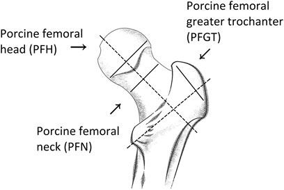
FIGURE 1. Anatomy of porcine trabecular bone and the corresponding regions selected for investigation. Samples were prepared from slices cut along the indicated directions (solid lines) and perpendicular to the respective main orientation (dashed lines) of each region.

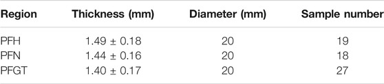
TABLE 1. Sample geometries and numbers for each of the investigated regions of porcine trabecular bone.

Electrical Impedance Spectroscopy

Samples were thawed at room temperature just prior to impedance measurements. To reduce the contribution of electrode polarization, extraneous liquid, covering the surfaces of the discs, was removed by wiping the samples with paper towels. Measurements were conducted in a solid test fixture (Agilent 16451B, Agilent Technologies Japan Ltd., Murotani, Kobeshinishiku, Japan) that was connected to an impedance analyzer (Agilent 4294A, Agilent Technologies Japan Ltd., Murotani, Kobeshinishiku, Japan). Impedance characteristics of the samples, i.e., resistance, R, and reactance, X, were recorded from 40 Hz to 5 MHz for 379 frequency points. The main components of the experimental setup are shown in Figure 2.

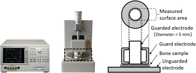
FIGURE 2. Impedance analyzer Agilent 4294A (left) and the connected test fixture Agilent 16451B (middle) with the dashed frame indicating details of the electrode arrangement (right).

The solid test fixture included three electrodes, i.e., an unguarded electrode, a guarded electrode, and a guard electrode to account for stray capacitances and, therefore, to reduce measurement errors. Ahead of the actual examinations, calibrations, including open and short compensation, were conducted according to the operation manuals [23, 24]. AC-excitation signals of 200 mV were applied for the experiments. Measurements were concluded within 2 min to limit the loss of moisture. Each sample was repositioned and examined four times to ensure reproducibility and stability of results.

Impedance, Z, can be written by using the following complex form:

where R describes the real part, i.e., resistance, and X the imaginary part, i.e., reactance (and j the imaginary square root of −1). Both parts were obtained from the impedance recorded by the Agilent analyzer. Dielectric and electrical properties, i.e., relative permittivity, ε_r, and conductivity, σ, were determined for each sample by considering the geometry, i.e., thickness, d, and surface area of the guarded electrode, A (Figure 2).

EIS Analysis Based on a Cole Model and a CPE

Impedance data were interpreted by an established Cole model for the bioimpedance analysis of tissues [25, 26], including bone [27]. Accordingly, measurements were related to an equivalent circuit model (Figure 3) and impedance spectra of the sample itself (Z_bone) fitted to the corresponding Cole model. Intrinsic characteristics of the samples were described by pertinent Cole parameters, i.e., resistance at very low frequency, R₀, resistance at infinite frequency, R_∞, characteristic time constant, τ, and a dimensionless parameter, α, with a value between 0 and 1 [28].

FIGURE 3. Equivalent circuit as basis for the analysis by a Cole model for the dielectric characterization of bone samples and contributions from EP, respectively.

For an aqueous system, a significant contribution from electrode polarization to the impedance at low frequencies is inevitable due to the development of electrical double layers at the interface between electrode and sample [19]. A proven method to account for the nonideal capacitance related to EP is the introduction of a constant phase element [19, 20]. The total impedance, distinguishing contributions from EP and from the actual bone sample, is then given by

with K being a measure for the magnitude of Z_ep, while α_ep and α are dimensionless factors (with values between 0 and 1), describing the dispersion for EP and bone, respectively.

Fitting of all impedance data was conducted by the function curve_fit, which is included in the Python library Scipy. As a known method to solve nonlinear least square problems and due to robustness, a Levenberg-Marquart (LM) algorithm was implemented together with the function. Consequently, Cole parameters could be estimated by minimizing the sum square of error functions between experimental data, y_exp, and results derived from the model, y_cole, as specified by

Hereby, n indicates the number of experimental data points, i.e., measurements. The goodness of fit between experimental data and model estimations was determined by the coefficients of determination (R²) as defined by

where the terms of y_exp and y_est corresponded to experimental and estimated data, respectively, and $\overline{y}$ to the average of the experimental results. Coefficients always showed values higher than 0.99 for all samples that were investigated.

Linear Discriminant Analysis

Different regions of trabecular bone, i.e., PFH, PFN, and PFGT, were identified and categorized by LDA with respect to different classes for each region which were reflecting characteristic properties, including for example permittivities and conductivities. The main idea of the LDA is to create or find an axis that can maximize the ratio of interclass to intraclass scatter and realize separation by finding linear combinations of input features [29]. As a supervised training model, LDA searches for the determining parameters by deriving confidence scores for each sample for a priori determined categories. The strength of the LDA is that categories can be predicted also for samples of unknown origin.

Discriminants of LDA were determined based on the dielectric variables, i.e., relative permittivity or conductivity, at the investigated frequencies. These were computed with the function LinearDisciminantAnalysis that was found in the Python library Scikit-learn. Coefficients for each discriminant (two discriminants were sufficient) were calculated, accordingly. A training dataset was defined from 80% of the samples that were analyzed for each region. The remaining 20% of the measurements were assigned to a test data set to verify the classification by the LDA.

Statistical Analysis

Mean values (mean) and standard deviations (SD) of Cole parameters were calculated by tools provided by Python libraries. A Pearson correlation was applied to determine the correlation coefficients between Cole parameters and pertinent sample compositions, e.g., resistance at higher frequencies, R_∞, and water content, φ. A t-test was applied to investigate the statistical significance of Cole parameters for the three regions.

Results

Dielectric and Electrical Properties

The mean values that were determined at different frequencies for permittivity and conductivity of different anatomical regions of bone (Figure 1), i.e., porcine femoral greater trochanter (PFGT), porcine femoral head (PFH), and porcine femoral neck (PFN), are shown in Figure 4. A representative example of respective errors, i.e., standard deviations, for samples from PFGT is presented in Supplementary Figure S1. Similar mean values and standard deviations for permittivity (Figure 4A) and conductivity (Figure 4B) were also observed for PFH and PFN. A strong frequency dependence was observed for both parameters, similar to previous reports [7, 9, 21]. At lower frequencies, values for the relative permittivity exceeded 10⁶ which fell off to values of less than 100 in the megahertz range. Only slightly higher values were found at lower frequencies (≤2.5 kHz) for PFH. No significant differences were observed between individual regions for frequencies of less than about 100 kHz while for higher frequencies the regions could be distinguished from each other. In contrast, the conductivity of PFGT was generally lower than for PFH and PFN. Conductivity was increasing for PFH and PFN samples from about 10 mS/m for lower frequencies and approaching 50 mS/m in the megahertz range. The values were higher for lower frequencies (≤7 kHz) for PFH but exceeded conductivity for PFN with further increasing frequency (>7 kHz). For PFGT samples, values reached only about 40 mS/m. Notable were also distinctively different frequency characteristics of the regional conductivities, which were, however, prone to large errors, i.e., variations, between individual samples as shown in Supplementary Figure S1. Regardless, conductivities increased at a much slower rate above 10 kHz, corresponding approximately to a frequency response that was similarly observed for permittivities.

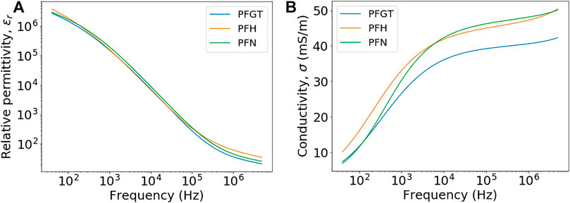
FIGURE 4. Mean values for samples from porcine femoral head (PFH), porcine femoral neck (PFN), and porcine femoral greater trochanter (PFGT): relative permittivities (A) and conductivities (B) as a function of frequencies.

For a more detailed understanding, especially in comparison with previous reports, permittivities and conductivities that were determined for individual samples from different regions of the bone were averaged together as “trabecular bone” and are presented for selected frequencies in Tables 2 and 3. Results that were determined for relative permittivity are in the range of assessments by Gabriel et al. who parameterized the values for trabecular bone by a 4-dispersion Cole model [27]. Similar characteristics have also been observed for human bone by Sierpowska et al. [7]. Only for lower frequencies (<1 kHz) was the permittivity of “trabecular bone” a little higher than described by Sierpowska et al. [7] or Gabriel et al. [27]. However, a better agreement was found with a later study with values of the same magnitude [9]. The values that were determined by Gabriel et al. [27] for conductivities are generally at least twice as high for higher frequencies and even five times higher for the lowest frequency when compared to our study. In comparison to the results by Sierpowska et al. [11], the changes that were observed are spanning a wider range, although for bovine bone the previous study by Sierpowska et al. [9] reports in general a much larger range for the results of individual frequencies. Corresponding values, although with weaker agreement, have also been documented for bovine bone [9].

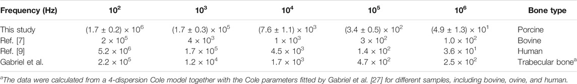
TABLE 2. Average values from all investigated bone samples, regardless of origin, for the relative permittivity at selected frequencies in comparison to previous studies.

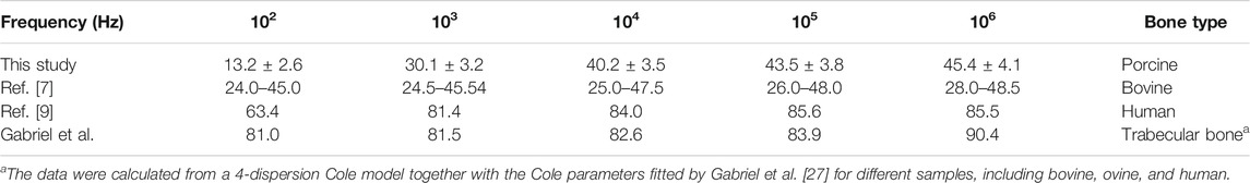
TABLE 3. Average values from all investigated bone samples, regardless of origin, for the conductivity at selected frequencies in comparison to previous studies.

EIS Analysis

A Cole model was developed on the basis of an equivalent circuit (cf. Figure 3) for a physical understanding of observed tissue properties. Permittivities and conductivities were reflected by distinct circuit elements, such as resistors and capacitors, in particular a constant phase element, accordingly. The modeling of recorded impedance spectra was conducted for altogether 64 independent samples. The data were fitted onto the model corresponding to (4) with the real part (resistance), Z′, and imaginary part (reactance), Z″, of the impedance, Z, represented in the complex Nyquist plane along horizontal and vertical axis, respectively. The typical example shown in Figure 5 demonstrates that the model describes the experimental data very well, with coefficients for the goodness of fit always higher than 99%. Correspondingly derived representative fitting results for dielectric parameters (data not shown), including permittivity and conductivity, further confirm the model.

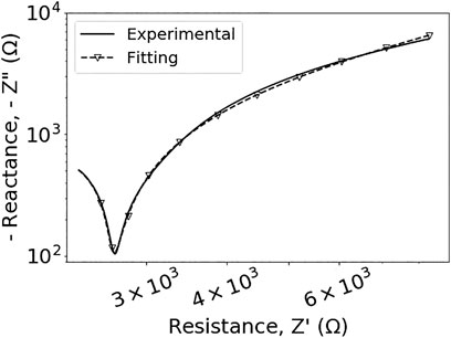
FIGURE 5. The representative experimental results for complex impedance, shown in Nyquist plot.

Physical traits were retained by typical parameters, i.e., R_∞, R₀, α, and τ, which describe the response of the equivalent circuit depending on different contributions of the tissue. These Cole parameters were determined for each sample. The mean values for the different investigated anatomical regions of the bone are shown in Table 4 together with standard deviations (±SD). The statistical analysis revealed that values of R₀, representing resistance at lowest frequencies, were similar for all regions (p > 0.05). No statistically significant differences were found for the characteristic time constant, τ, although distinctions between mean values were indicated (p > 0.05). Conversely, the different parts of the bone differ significantly in values for R_∞ (p < 0.05) and even more for α (p < 0.01). The resistance at high frequencies, expressed by R_∞, was highest for PFGT, followed by distinctively lower values for PFH and successively PFN. The same trend was observed for the shape parameter, α, with the highest values obtained again for PFGT-samples, lower numbers for samples from the PFN, and the smallest values for PFH-specimen. Cole parameters for electrode polarization showed no significant differences regardless of the regions (Supplementary Table S1).

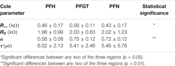
TABLE 4. Cole parameters (mean ± SD) for different regions of porcine trabecular bone.

Correlation Between Resistance at Higher Frequencies and Water Content

The bulk electrical properties of tissues are determined by their structure and composition. Especially water with a high relative permittivity was expected to affect different parameters and in particular the resistance at higher frequencies, R_∞. Therefore, Pearson correlation coefficients were determined for the relation between R_∞ and water content, φ, of the samples. Results for the different samples are presented together with regression coefficients, r, in the scatter plots that are shown in Figure 6. The shaded area indicates the 95% confidence intervals for the regressions.

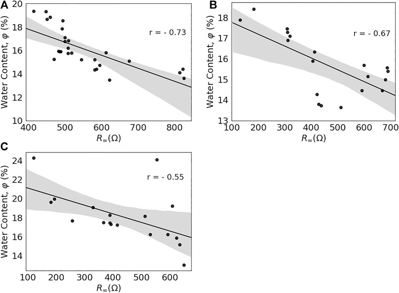
FIGURE 6. Relationship between R_∞ and water content, φ, for individual samples from the porcine greater trochanter, PFGT (A), porcine femoral head, PFH (B), and porcine femoral neck, PFN (C).

Overall, water content decreased as R_∞ increased. A strong correlation between R_∞ and φ was observed for PFGT (Figure 6A), PFH (Figure 6B), and PFN (Figure 6C), with the highest level of confidence for PFGT (r = 0.73), followed by PFH (r = 0.67) and PFN (r = 0.55). Individual larger residuals for some outliers were observed for PFH and PFN. The relation between both parameters can be described by the following for PFGT, PFH, and PFN, respectively:

LDA Based on Electrical Properties

The wish for a better and more reliable discrimination of different anatomical regions and in perspective a more reliable categorization of samples of unspecified origin and condition prompted the application of LDA as supplementary method. With this approach, features (dimensions) can be reduced, samples classified and the classification visualized with respect to defined categories. A caveat of the method is the required training. Features, i.e., relative permittivity and conductivity, were considered for different frequencies and defined the input training data for categories of interest, i.e., PFGT, PFH, and PFN. The data were then transformed into a new 2-feature (linear discriminant) dataset. Each feature contributes to the discrimination of different regions, although to a different degree. The primary discriminant (LD1) generally carries more information than the second (LD2). The results of the transformation into LD1 and LD2 and the associated categorization of individual samples are shown in Figure 7. For the conducted LDA, based on relative permittivity (Figure 7A), LD1 and LD2 contributed with 66.59 and 33.41% to the classification, while the same features were responsible with 81.07 and 18.93% for a discrimination based on conductivity (Figure 7B). In both cases were the different anatomical regions clearly distinguished from each other and most samples could be assigned to their respective categories with only a few exceptions.

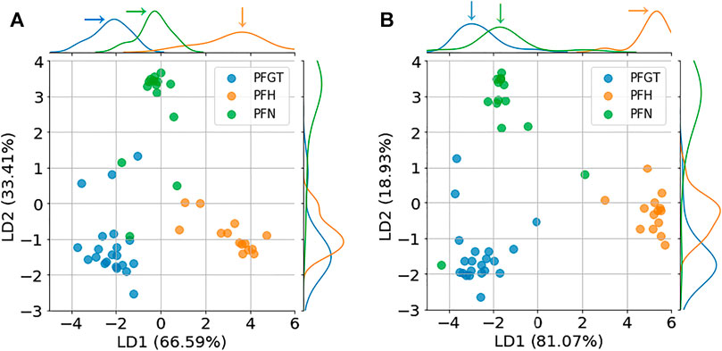
FIGURE 7. Discrimination of samples from different regions after LDA based on relative permittivity (A) and conductivity (B). LDA discriminants, LD1 and LD2, determined the different contributions to the classes that can be identified for porcine greater trochanter (PFGT), porcine femoral head (PFH), and porcine femoral neck (PFN).

The contribution to the distinction between different classes, that were reflected in LD1 and LD2, can be expressed by their respective coefficients. Larger coefficients signify a more substantial contribution to differences. The coefficients vs. frequency for each LDA component are shown in Supplementary Figure S2. For the analysis based on relative permittivity (Supplementary Figure S2A), for example, coefficients for both LD1 and LD2 were higher for higher frequencies (≥1.1 × 10⁵ Hz), indicating more weight for the obtained distinction of regions for this frequency range.

Corresponding peaks in the distribution densities (pointed out in the figure by arrows) suggest typical representations for the different regions, which can be exploited specifically in clinical applications or in further studies.

The different categories, with respect to LD1 and LD2, were derived from about 80% of the investigated samples of known origin. These specimens constituted the training data set for a subsequent application of method and algorithms towards unknown samples. The remaining 20% of the available data were then deliberately considered as ‘unspecific’ to verify the approach. The classification of the samples was based on relative permittivity. At the end, the assignment by LDA was compared with the actual anatomical origin of the test samples. The results of the comparison between prediction (output data) and actual origin (input data) are presented in Figure 8.

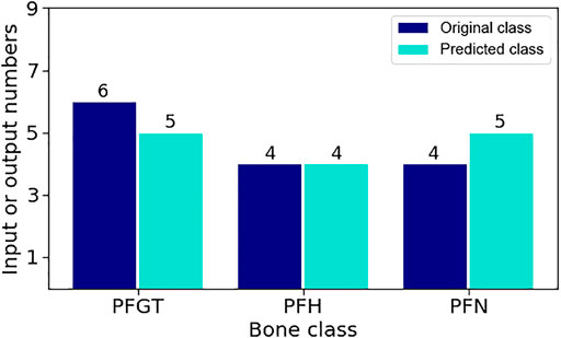
FIGURE 8. Comparison for the assignment of a priori undetermined samples by the LDA model. Samples were designated to their correct class with an accuracy of 92.9%. Only one PFGT-sample was wrongly identified as PFN-tissue.

Except for one PFGT sample, which was wrongly identified as PFN tissue, all other samples were correctly assigned to their respective categories. Hence, LDA achieved a rather precise discrimination of different bone tissues with an accuracy of 92.9%. The result could conceivably be improved by further or continuous training of the method.

Discussion

Dielectric and Electrical Properties of Porcine Trabecular Bone

Impedance Analysis of Bone Tissue

The impedance properties of the samples measured between parallel plate electrodes were investigated at frequencies from 40 Hz to 5 MHz under an AC-signal stimulus. As for any other system with electrodes that are in contact with an aqueous material, contributions from electrode polarization to the measurements are inevitable [19]. Different approaches have been developed to reduce the effect experimentally or correct results for EP analytically. Sierpowska et al. [7] used stainless steel electrodes for their studies, while other efforts relied on solid gold electrodes [30]. Gabriel et al. parameterized dielectric properties for trabecular bone based on literature data without regard of electrode materials. For the presented investigation, no information could be obtained for the electrode material of the commercial system, i.e., Agilent 16451B (Figure 2). However, in comparison to other systems, a third electrode, i.e., guard electrode, is implemented to reduce stray capacities [24].

In contrast to the work of Sirepowska et al. [7], the application of a thin layer of conductive gel onto the samples to improve the contact with the electrodes was abstained. On the one hand, the gel does apparently not provide a significant advantage to reduce EP [16]. On the other hand, the gel could penetrate into the highly porous material of the bone and could either enhance EP or at least hinder an interpretation of the actual electrical properties of the tissue itself. Instead, samples were kept moist and wiped dry of excess liquid prior to the measurements. This assured a good contact and limited additional contributions to the impedance which were not related to the actual composition of the bone.

The comparison with other studies, as shown in Tables 2 and 3, confirmed that the equipment and the developed procedures addressed EP sufficiently, with reproducible results that were for corresponding average values on the same order and often even with smaller errors (Supplementary Figure S1). Results shown in Dielectric and Electrical Properties were in general in the same order of magnitude with respect to permittivity and conductivity for “trabecular bone” as values that were reported by Sierpowska et al. and Gabriel et al. Discrepancies are presumably due to the individual procedures and specific restrictions of the actual systems and methods as well as differences in the consideration of EP. For the studies by Gabriel et al., it has to be pointed out that data for different specimens, e.g., bovine, ovine, and human bone, were summarized and therefore represented a more general assessment. That means different specimens, pathological conditions, such as age and gender, and different anatomical regions, also contributed to the discrepancies between different studies. This pronounces the need for an improved characterization of trabecular bone with respect to patient-specific conditions. Considering the above-mentioned factors, the presented values were of similar quality to the previous studies, but the comparison also indicates general limitations of the approach.

Conductivity and Relative Permittivity for Different Bone Regions

While previous studies have treated trabecular bone as material with uniform properties, this approach is not sufficient for the evaluation of patient-specific differences or local variation of electrical parameters, as it is important for planning specific therapies by electrical stimulation. Differences for the anatomical regions of porcine trabecular bone that were accordingly investigated, were in particular observed for conductivity (Figure 4B).

All samples were carefully cleaned and residual blood and soft tissue, such as fat and marrow, were removed ultrasonically or by solvents. Consequently, any differences should be attributable to the remaining mineral content and the microstructure. Voids in the thin samples (1–2 mm) were filled with water. A clear linear relationship between water content, φ, and the Cole-parameter, R_∞, as an indicator for the corresponding conductivity, could in fact be observed for every individual anatomic region (Figure 6, p < 0.01). Notably, Sierpowska et al. [14] found no significant difference in water content among sample sites. However, the group found a strong correlation between water content and electrical properties for the averages that were derived for the entire bone. A higher spatial resolution for the different regions of complex trabecular bone should eventually be able to resolve the perceived discrepancies. Conversely, the method itself proved successful to resolve even small changes in water content and correlate them with electrical parameters. This encourages future applications also towards other tissue constituents, such as fat or mineral content and together with a reliable classification overall “bone quality”.

Significant variation of water content for the investigated regions (p < 0.01) also indicated differences between these regions, resulting from their individual microstructure, e.g., bone volume fraction (BV/TV), which characterizes bone volume per unit tissue (sample) volume. Notably, especially for PFN, water content could be varied within a slightly higher range than for PFH and PFGT. This indicated indirectly that either more voids or larger voids were present in the microstructure and could be filled with water. However, since this by itself does not explain the otherwise very similar results for conductivity and relative permittivity for all regions (Figure 4), it could be assumed that the detailed distribution and possible variations in density in the bone matrix itself need to be considered. Previous studies have shown a correlation between bone density and dielectric properties. A linear correlation between BV/TV and conductivity for comparable frequencies was also found by Balmer et al. [16] for 100 kHz and by Sierpowska et al. [14] for 1.2 MHz. The relation, in general, was frequency dependent, i.e., especially a linear correlation cannot easily or necessarily be observed at other frequencies. However, for an identified appropriate value were the respective slopes a good indicator to conclude from conductivity on characteristics of the microstructure. How water content and the contribution of other components can also be included in an eventually comprehensive analysis has yet to be determined and is the important objective of future studies.

Modeling of Electrical Properties of Bone by an Equivalent Circuit

Another method that is often used in conjunction with Cole models is the analysis of impedance responses of materials, including bone tissues, by an equivalent circuit. By accounting for interfacial phenomena with a constant phase element, the electrical properties of a system can be described by an equivalent circuit with the CPE in series with a Cole model as shown in Figure 3. The advantage of the approach is that different components of a system can be related to specific physical characteristics or circuit elements. This includes conductivities and relative permittivities, which are reflected in resistive and capacitive elements. Moreover, other characteristic parameters provided additional insight into the electrical properties of a complex material. An instructive simplification of a Cole model, in comparison with other models, is often the lower number of parameters [31]. Pertinent parameters of such a model are in particular the resistance at lowest and highest frequencies, i.e., R₀ and R_∞, the characteristic time constant, τ, and the shape parameter, α. The value of the latter is associated with intrinsic relaxation processes and the inhomogeneity of tissues [32]. These parameters are often used to assess pathological conditions, i.e., distinguishing normal from cancerous tissue [26, 31]. They can also be exploited to discriminate osteopathic tissue from healthy bone with respect to microstructure [15].

For biological tissues, the heterogeneous characteristic dominantly results in interfacial polarizations, i.e., Maxwell-Wagner effect [33]. This effect, that arises from the charging of interfaces between different materials, was possibly due to abundant interfaces between bone and water. The interfacial polarization is more pronounced for highly homogeneous and anisotropic materials [34], such as bone [30, 35]. In addition, possible legacy components [36], e.g., blood vessels, collagen, and cells, may present additional remaining interfaces. The polarization is reflected in various dispersion processes, in particular at low frequencies.

No significant differences (p > 0.05) were found or could rather not be resolved by these parameters, for R₀ and τ for the three investigated different anatomical regions (Table 4). This is not necessarily surprising, if the microstructure and tissue composition, which are described implicitly by τ, and the associated extracellular resistance, expressed by R₀, are in fact very similar to the adjacent bone regions [14]. However, respective differences could be successfully resolved by α and R_∞. It should be mentioned that Cole parameters to describe EP, including K and α_ep, revealed no significant differences (Supplementary Table S1) that could be associated with sample roughness due to differences in microstructure or water content. This indicated that contribution from EP was not much distinct to the samples for each different region.

Notable differences were observed for the shape parameter, α (Table 4). Average values for α are for all regions well within the range that was reported by previous studies [25, 27]. Novel is, however, the finding that even very similar regions can be distinguished with high statistical significance (p < 0.01). Responsible could be specific inhomogeneities and associated relaxation processes related to the Maxwell-Wagner effect, as a result of the charging of interfaces between bone and water [35] and possibly even cell membranes [33]. It should be mentioned that these processes could so far not be directly observed from impedance spectroscopy.

The resistance at highest frequencies, R_∞, is another parameter that revealed significant differences between the different regions (p < 0.05). Values describe primarily the ability of electrical currents to cross membranes and penetrate cell membranes at higher frequencies. The microstructure of trabecular bone is primarily determined by extracellular hydroxyapatite with an inherent high resistance. Most cell membranes were possibly destroyed during the preparation and freezing process. Major current pathways are, therefore, determined by fluid in separated compartments of the hydroxyapatite microstructure. A denser, more calcified tissue matrix corresponds to lesser space that could be filled and more relevant interfaces in general. Changes of R_∞ could therefore in particular describe water content of the samples (Figure 6). In association with the correlation between conductivity (σ) and bone density (BV/TV), R_∞, hence, provided indirectly information on the microstructure (cf. (5–7)). Similar conclusions on the correlation between electrical properties and microstructure were already drawn by Sierpowska et al. [10]. The correlation between electrical parameters and the microstructure and composition of bone tissue still need to be further investigated.

A discrimination of different regions by a Cole model alone is ambitious and often prone to fitting errors. Other studies have further argued that parameters are inherently variable, even when deduced from repetitive measurements on the same sample [37]. The approach can be improved and risks in the analysis were mitigated by a comparison of results from alternative models and by evaluations that complement a Cole-analysis, such as LDA.

Linear Discriminant Analysis of Dielectric Properties

LDA offers another perspective for the classification of different tissue types that were characterized already by a Cole model. From the comparison of the classification that is obtained by both approaches, the differentiation of anatomical regions can be verified, and in particular fitting errors of the Cole analysis alleviated.

LDA as a supervised method differs from unsupervised methods, such as principle component analysis (PCA) that does not consider the category information [38]. Accordingly, the analysis by PCA (data not shown) did not achieve an even reluctantly accepted discrimination between the different bone regions, while LDA did. The advantage of the higher classification efficiency has already been applied as a method in other bioimpedance studies [37, 39]. In the LDA, observed properties for a set of measurements were transformed into a new frame of reference of alternative variables, i.e., linear discriminants (LDs). Accordingly, an LDA based on relative permittivity or conductivity could effectively discriminate the investigated anatomical regions of porcine trabecular bone, i.e., PFH, PFN, and PFGT. The different classes were clearly separated in the plane of the linear discriminants LD1 and LD2 (Figure 7), confirming intrinsic differences of underlying dielectric properties. Correspondingly, clearly separated peaks could be identified in the respective density distributions, for the typical representations of each group. This distinction based on permittivity, for example, was more obvious for LD1 than for LD2 with 66.6 and 33.4%, respectively.

The results for coefficients for LD1 and LD2 could serve as an informative interpretation for understanding their characteristics and for a related Cole analysis. For example, contributions at lower frequencies (≤10⁵ Hz) could be due to α-dispersion as a result of interfacial polarization [33]. The process could be overlapped by contributions from EP [19]. However, the interpretation on this process would be greatly hindered by the similar effect of EP, as indicated by the insignificance of Cole parameters for EP, i.e., K and α_ep (Supplementary Table S1). The different coefficients of both LDs at middle and higher frequencies further suggested that the discrimination that was found for the shape parameter, α, was possibly caused by different β- dispersion processes (up to MHz) [34]. The LDA based on conductivity (Supplementary Figure S2B) can be interpreted by the following similar arguments.

Although a separation and classification of the different regions were also possible from an evaluation of relative permittivity and conductivity by the Cole model (Figure 4), the respective discrimination was not as robust. Conversely, the classification by LDA that was based on relative permittivity or conductivity suggested dielectric properties and responses that cannot be intuitively derived from impedance spectroscopy. While different regions could also be distinguished by the Cole parameters α and R_∞, an LDA based on these parameters did not provide any meaningful discrimination (data not shown).

A particular strength of the LDA, as a statistical method, is the possibility to characterize tissues with steadily improving accuracy with increasing numbers of samples that have been categorized. The predictions for deliberately unspecified samples showed a success of 92.9% (Figure 8). Consequently, the advantage of LDA is the classification of tissues in clinical settings, e.g., estimating the severity of osteoporosis. With respect to the basic understanding of electrical properties of tissues, LDA provides also a means to identify outliers in concurrent evaluations, which may result from sample preparation or measurement errors. Accordingly, ambiguous results outside the bounds of the representations for PFGT and PFN, as they are shown in Figure 7 for the classification of samples, could be excluded from the analysis by the Cole model to deduce more reliable estimates on the typical or representative dielectric parameter of the respective tissues.

Although a finer discrimination based on the dielectric and electrical properties can be obtained from LDA, it has to be kept in mind that the derivation of relative permittivity or conductivity and a relation to any physical meaning are not possible from the approach by itself. Therefore, LDA and the Cole model complement each other, with LDA promoting the interpretation of impedance measurements with respect to differences in the electrical properties of tissues.

Conclusion

The investigation showed the possibility to distinguish similar but anatomically still different bone tissues from each other from the analysis of impedance responses by a Cole model. While this is feasible from relative permittivities and conductivities alone, the Cole parameters for the resistance at higher frequency, R_∞, and foremost the shape parameter, α, provided further and higher confidence. Notably, α, but also other Cole parameters can be related to composition and microstructure of bone. On this basis, detailed models that are relating distinct physiological states with electrical properties could be developed, e.g., for osteoporosis.

Since a Cole analysis is inherently prone to fitting errors, the respective discrimination can be supplemented by an LDA, which is able to verify the classification and assessment based on relative permittivity or conductivity. The benefit for the development of more precise models for bone structures, based on typical representations of different regions and conditions of bone, is obvious. This improved characterization would also be beneficial for diagnosis of patient-specific differences. These could in particular guide the development and application of therapies for electrical stimulation. Individual dielectric parameters will determine the distribution of applied electric fields and can be adjusted in their magnitude accordingly. Combining the results from EIS and Cole analysis, an advanced interpretation on the discrimination for regional difference can be achieved, e.g., from the coefficients at the investigated frequencies. Corollary, the LDA of impedance data further offers a novel approach for clinical diagnostics by classifying tissue conditions with respect to their pathological conditions. Moreover, the method, combining Cole analysis and LDA, offers the possibility to interpret the characteristics for different biomaterials. The predictive power of the method would increase if large data sets can be provided.

Data Availability Statement

The original contributions presented in the study are included in the article/Supplementary Material; further inquiries can be directed to the corresponding author.

Ethics Statement

The animal study was reviewed and approved by the Animal Care Committee of the Leibniz Institute of Farm Animal Biology. Written informed consent was obtained from the owners for the participation of their animals in this study.

Author Contributions

WW performed the experiment and data analysis and wrote the manuscript. FS contributed various ideas and suggestions on the manuscript. JK reviewed and edited the manuscript and oversaw the project. All authors contributed to manuscript revision and read and and approved the submitted version.

Funding

This work was supported by the Deutsche Forschungsgemeinschaft (DFG, German Research Foundation)–SFB 1270/1–299150580.

Conflict of Interest

The authors declare that the research was conducted in the absence of any commercial or financial relationships that could be construed as a potential conflict of interest.

Acknowledgments

WW would especially like to thank Michael Oster from Leibniz Institut for Farm Animal Biology (FBN, Dummerstorf) and Michael Sämann from the University of Rostock for their assistance with sample procurement and preparation.

Supplementary Material

The Supplementary Material for this article can be found online at: https://www.frontiersin.org/articles/10.3389/fphy.2020.576191/full#supplementary-material.

References

1. Bässgen K, Westphal T, Haar P, Kundt G, Mittlmeier T, Schober HC. Population-based prospective study on the incidence of osteoporosis-associated fractures in a German population of 200,413 inhabitants. J Public Health (2012) 35:255–61. doi:10.1093/pubmed/fds076
2. Svedbom A, Hernlund E, Ivergård M, Compston J, Cooper C, Stenmark J, et al. Osteoporosis in the European Union: a compendium of country-specific reports. Arch Osteoporos (2013) 8:137. doi:10.1007/s11657-013-0137-0
3. Yonemori K, Matsunaga S, Ishidou Y, Maeda S, Yoshida H. Early effects of electrical stimulation on osteogenesis. Bone (1996) 19:173–80. doi:10.1016/8756-3282(96)00169-X
4. Leppik LP, Froemel D, Slavici A, Ovadia ZN, Hudak L, Henrich D, et al. Effects of electrical stimulation on rat limb regeneration, a new look at an old model. Sci Rep (2015) 5:18353. doi:10.1038/srep18353
5. Khalifeh JM, Zohny Z, MacEwan M, Stephen M, Johnston W, Gamble P, et al. Electrical stimulation and bone healing: a review of current technology and clinical applications. IEEE Rev Biomed Eng (2018) 11:217–32. doi:10.1109/RBME.2018.2799189
6. Williams PA, Saha S. The electrical and dielectric properties of human bone tissue and their relationship with density and bone mineral content. Ann Biomed Eng (1996) 24:222–33. doi:10.1007/BF02667351
7. Sierpowska J, Töyräs J, Hakulinen MA, Saarakkala S, Jurvelin JS, Lappalainen R. Electrical and dielectric properties of bovine trabecular bone–relationships with mechanical properties and mineral density. Phys Med Biol (2003) 48:775. doi:10.1088/0031-9155/48/6/306
8. Raben H, Kämmerer PW, Bader R, van Rienen U. Establishment of a numerical model to design an electro-stimulating system for a porcine mandibular critical size defect. Appl Sci (2019) 9:2160. doi:10.3390/app9102160
9. Sierpowska J, Hakulinen MA, Töyräs J, Day JS, Weinans H, Jurvelin JS, et al. Prediction of mechanical properties of human trabecular bone by electrical measurements. Physiol Meas (2005) 26:S119–31. doi:10.1088/0967-3334/26/2/012
10. Sierpowska J, Hakulinen MA, Töyräs J, Day JS, Weinans H, Kiviranta I, et al. Interrelationships between electrical properties and microstructure of human trabecular bone. Phys Med Biol (2006) 51:5289–303. doi:10.1088/0031-9155/51/20/014
11. Sierpowska J, Lammi MJ, Hakulinen MA, Jurvelin JS, Lappalainen R, Töyräs J. Effect of human trabecular bone composition on its electrical properties. Med Eng Phys (2007) 29:845–52. doi:10.1016/j.medengphy.2006.09.007
12. Kosterich JD, Foster KR, Pollack SR. Dielectric permittivity and electrical conductivity of fluid saturated bone. IEEE Trans Biomed Eng (1983) 30:81–6. doi:10.1109/tbme.1983.325201
13. Gabriel C, Gabriel S, Corthout E. The dielectric properties of biological tissues: I. literature survey. Phys Med Biol (1996) 41:2231–49. doi:10.1088/0031-9155/41/11/001
14. Sierpowska J. Electrical and dielectric characterization of trabecular bone quality. [PhD thesis]. Kuopio (Finland): University of Kuopio (2007).
15. Amin B, Elahi MA, Shahzad A, Porter E, McDermott B, O’Halloran M. Dielectric properties of bones for the monitoring of osteoporosis. Med Biol Eng Comput (2019) 57:1–13. doi:10.1007/s11517-018-1887-z
16. Balmer TW, Vesztergom S, Broekmann P, Stahel A, Büchler P. Characterization of the electrical conductivity of bone and its correlation to osseous structure. Sci Rep (2018) 8:8601. doi:10.1038/s41598-018-26836-0
17. Gerasimenko T, Nikulin S, Zakharova G, Poloznikov A, Petrov V, Baranova A, et al. Impedance spectroscopy as a tool for monitoring performance in 3D models of epithelial tissues. Front Bioeng Biotechnol (2019) 7:474. doi:10.3389/fbioe.2019.00474
18. Grimnes S, Martinsen OG. Cole electrical impedance model–a critique and an alternative. IEEE Trans Biomed Eng (2004) 52:132–5. doi:10.1109/TBME.2004.836499
19. Ishai PB, Talary MS, Caduff A, Levy E, Feldman Y. Electrode polarization in dielectric measurements: a review. Meas Sci Technol (2013) 24:102001. doi:10.1088/0957-0233/24/10/102001
20. Kalvøy H, Johnsen GK, Martinsen OG, Grimnes S. New method for separation of electrode polarization impedance from measured tissue impedance. Open Biomed Eng J (2011) 5:8–13. doi:10.2174/1874120701105010008
21. Gabriel S, Lau RW, Gabriel C. The dielectric properties of biological tissues: II. measurements in the frequency range 10 Hz to 20 GHz. Phys Med Biol (1996) 41:2251–69. doi:10.1088/0031-9155/41/11/002
22. McAdams ET, Jossinet J. Problems in equivalent circuit modelling of the electrical properties of biological tissues. Bioelectrochem Bioenerg (1996) 40:147–52. doi:10.1016/0302-4598(96)05069-6
23.Agilent. Agilent 4294A precision impedance analyzer operational manual. Available at: http://literature.cdn.keysight.com/litweb/pdf/04294-90060.pdf. (Accessed December 2019)
24.Keysight. Keysight 16451B dielectric test fixture operation and service manual. Available at: http://literature.cdn.keysight.com/litweb/pdf/16451-90020.pdf. (Accessed December 2019)
25. Peyman A, Gabriel C. Cole-Cole parameters for the dielectric properties of porcine tissues as a function of age at microwave frequencies. Phys Med Biol (2010) 55:N413–9. doi:10.1088/0031-9155/55/15/N02
26. Laufer S, Ivorra A, Reuter VE, Rubinsky B, Solomon SB. Electrical impedance characterization of normal and cancerous human hepatic tissue. Physiol Meas (2010) 31:995–1009. doi:10.1088/0967-3334/31/7/009
27. Gabriel S, Lau RW, Gabriel C. The dielectric properties of biological tissues: III. Parametric models for the dielectric spectrum of tissues. Phys Med Biol (1996) 41:2271. doi:10.1088/0031-9155/41/11/003
28. Shi F, Steuer A, Zhuang J, Kolb JF. Bioimpedance analysis of epithelial monolayers after exposure to nanosecond pulsed electric fields. IEEE Trans Biomed Eng (2019) 66:2010–21. doi:10.1109/TBME.2018.2882299
29. Giana FE, Bonetto FJ, Bellotti MI. Assay based on electrical impedance spectroscopy to discriminate between normal and cancerous mammalian cells. Phys Rev E (2018) 97:032410. doi:10.1103/PhysRevE.97.032410
30. Haba Y, Wurm A, Köckerling M, Schick C, Mittelmeier W, Bader R. Characterization of human cancellous and subchondral bone with respect to electro physical properties and bone mineral density by means of impedance spectroscopy. Med Eng Phys (2017) 45:34–41. doi:10.1016/j.medengphy.2017.04.002
31. Stoneman MR, Kosempa M, Gregory WD, Gregory CW, Marx JJ, Mikkelson W, et al. Correction of electrode polarization contributions to the dielectric properties of normal and cancerous breast tissues at audio/radiofrequencies. Phys Med Biol (2007) 52:6589–604. doi:10.1088/0031-9155/52/22/003
32. Ramírez-Chavarría RG, Sánchez-Pérez C, Matatagui D, Qureshi N, Pérez-García A, Hernández-Ruíz J. Ex-vivo biological tissue differentiation by the distribution of relaxation times method applied to electrical impedance spectroscopy. Electrochim Acta (2018) 276:214–22. doi:10.1016/j.electacta.2018.04.167
33. Kuang W, Nelson SO. Low-frequency dielectric properties of biological tissues: a review with some new insights. Trans ASAE (1998) 41:173–84. doi:10.13031/2013.17142
34. Foster KR, Schwan HP. Dielectric properties of tissues and biological materials: a critical review. Crit Rev Biomed Eng (1989) 17:25–104.
35. Kang H, Hou Z, Qin QH. Experimental study of time response of bending deformation of bone cantilevers in an electric field. J Mech Behav Biomed Mater (2018) 77:192–8. doi:10.1016/j.jmbbm.2017.09.017
36. Bhardwaj P, Rai DV, Garg ML, Mohanty BP. Potential of electrical impedance spectroscopy to differentiate between healthy and osteopenic bone. Clin Biomech (2018) 57:81–8. doi:10.1016/j.clinbiomech.2018.05.014
37. Nejadgholi I, Caytak H, Bolic M, Batkin I, Shirmohammadi S. Preprocessing and parameterizing bioimpedance spectroscopy measurements by singular value decomposition. Physiol Meas (2015) 36:983–99. doi:10.1088/0967-3334/36/5/983
38. Shi F, Zhuang J, Kolb JF. Discrimination of different cell monolayers before and after exposure to nanosecond pulsed electric fields based on Cole-Cole and multivariate analysis. J Phys D Appl Phys (2019) 52:495401. doi:10.1088/1361-6463/ab40d7
Keywords: electrical impedance spectroscopy, osseous tissue, permittivity, conductivity, bone tissue discrimination
Citation: Wei W, Shi F and Kolb JF (2021) Impedimetric Analysis of Trabecular Bone Based on Cole and Linear Discriminant Analysis. Front. Phys. 8:576191. doi: 10.3389/fphy.2020.576191
Received: 10 July 2020; Accepted: 22 December 2020;
Published: 11 February 2021.
Edited by:
Udo Jochen Birk, University of Applied Sciences Graubünden, SwitzerlandReviewed by:
Uwe Pliquett, Institut für Bioprozess-und Analysenmesstechnik (IBA), GermanyIndira Chatterjee, University of Nevada, Reno, United States
Copyright © 2021 Wei, Shi and Kolb. This is an open-access article distributed under the terms of the Creative Commons Attribution License (CC BY). The use, distribution or reproduction in other forums is permitted, provided the original author(s) and the copyright owner(s) are credited and that the original publication in this journal is cited, in accordance with accepted academic practice. No use, distribution or reproduction is permitted which does not comply with these terms.
*Correspondence: Juergen F. Kolb, juergen.kolb@inp-greifswald.de