Toward Waveguide-Based Optical Chromatography
 Antonio A. R. Neves
 Wendel L. Moreira2
  Adriana Fontes
 Tijmen G. Euser
 Carlos L. Cesar
- 1Centro de Ciências Naturais e Humanas, Universidade Federal Do ABC (UFABC), Santo André, Brazil
- 2Tratamento de Dados Geofísicos, Tecnologia e Processamento de Geologia e Geofísica, Exploração, Petrobras - Petróleo Brasileiro S.A., Rio de Janeiro, Brazil
- 3Departamento de Biofísica e Radiobiologia, Universidade Federal de Pernambuco (UFPE), Recife, Brazil
- 4NanoPhotonics Centre, Cavendish Laboratory, Department of Physics, University of Cambridge, Cambridge, United Kingdom
- 5Departamento de Física, Universidade Federal Do Ceará (UFC), Fortaleza, Brazil
- 6Instituto de Física “Gleb Wataghin”, Departamento de Eletrônica Quântica, Universidade Estadual de Campinas (UNICAMP), Campinas, Brazil
- 7National Institute of Science and Technology on Photonics Applied to Cell Biology (INFABIC), Campinas, Brazil
We report analytical expressions for optical forces acting on particles inside waveguides. The analysis builds on our previously reported Fourier Transform method to obtain Beam Shape Coefficients for any beam. Here we develop analytical expressions for the Beam Shape Coefficients in cylindrical and rectangular metallic waveguides. The theory is valid for particle radius a ranging from the Rayleigh regime to large microparticles, such as aerosols like virus loaded droplets. The theory is used to investigate how optical forces within hollow waveguides can be used to sort particles in “optical chromatography” experiments in which particles are optically propelled along a hollow-core waveguide. For Rayleigh particles, the axial force is found to scale with a6, while the radial force, which prevents particles from crashing into the waveguide walls, scales with a3. For microparticles, narrow Mie resonances create a strong wavelength dependence of the optical force, enabling more selective sorting. Several beam parameters, such as power, wavelength, polarization state and waveguide modes can be tuned to optimize the sorting performance. The analysis focuses on cylindrical waveguides, where meter-long liquid waveguides in the form of hollow-core photonic crystal fibers are readily available. The modes of such fibers are well-approximated by the cylindrical waveguide modes considered in the theory.
1 Introduction
Since Ashkin’s pioneering paper [1], Optical Tweezers (OT) have opened up the possibility to perform micro- and nanoscale non–contact mechanical manipulation and measurements on particles in the nano-micron scale. Single and multiple optical beams can hold, stretch, and compress particles, filaments, vesicles in a suspension, enabling novel applications such as optical force spectroscopy of microspheres [2, 3]. The room temperature force sensitivity of OT based techniques ranges from 20 fN [4] to 200 pN [5], making this tool ideal to handle particles in the biological micro–environment. Single–beam optical tweezers have allowed the development of several applications in life science, and use optical forces created by a tightly focused laser beam not only to manipulate micron to nanometer–sized structures, but also to measure their mechanical properties [6–8]. The single–beam optical tweezers require gradient forces that exceed scattering forces, a condition usually met with in the case of small differences between medium/particle refractive indexes. This situation is commonly found in aqueous solutions, but not in air or vacuum. The Brownian motion sets the limit for the size of the smallest particle that can be trapped, although at low temperatures (not compatible with live cells), it is possible to even optically trap atomic gases [9]. The success of the single–beam optical tweezers has encouraged the development of new, complementary optical trapping configurations, including optical chromatography, a method that combines the use of optical forces to manipulate and size–select particles in microfluidic systems [6].
Optical chromatography was initially proposed by Imasaka et al. in 1995 [10]. Their approach consisted of mildly focusing a laser beam into a solution containing particles that are counter–flowing coaxially with a capillary. When in equilibrium, there is a balance between the laser scattering force and the drag force from the fluid medium. A challenge in this configuration is to keep the laser beam aligned at the center of the of capillary. Since these pioneering experiments, optical chromatography has led to a range of different applications, for example: to visualize immunological reactions by flowing a sample of antigens past optically–trapped beads that are coated with antibodies. Selective binding changes the effective size of the particles an thus their retention distance. This allowed to determine antigen concentrations in the range from nanomolar to nanograms per milliliter [11]. Optical chromatography can also be used to separate same–sized particles of different refractive indices [12], and be combined with microfluidic channels with well–defined velocity flow patterns [13]. This approach was used to measure low concentrations of anthrax bacteria, by accumulating them from a flow in an optical trap [14]. Further improvements of the technique include hydrodynamic focusing, enabling the separation of equal–sized microsphere differing only 0.1 in refractive index [15]. Further optical chromatography and other optical sorting strategies were summarized in a recent review [6].
Optical chromatography requires a good understanding of the forces acting on the analyzed particles. Initial models were based on geometrical–optics models, and identified analogies with separation parameters for conventional chromatography such as: retention distance, selectivity, dynamic range, theoretical plate number, and resolution [16]. Using a focused Gaussian beam, the retention distance can be related to the Rayleigh length, and can be shown to scale as the square root of particle size. The selectivity in chromatography is directly related to the slope of the retention distance vs. particle size, which can be tuned by carefully changing the laser power and the flow velocity. The dynamic range, defined as the ratio between the maximum and minimum particle size that can be analyzed, is ultimately limited by the size-range of particles that can be trapped. The theoretical plate number, another chromatography parameter, determines the separation efficiency in optical chromatography. In the case of optical traps, this is typically limited by Brownian fluctuations and instrumental noise. Finally, the resolution of particle separation can be determined from the theoretical plate number and selectivity. In theory, particles can be resolved if they differ from at least 0.4% in size [16].
A more recent approach to optical separation uses hollow–core photonic crystal fibers with core diameters between 10 and 30 μm, to optically trap and guide particles along a length of fiber [17]. Advantages are the presence of well–defined waveguide modes, that are well-approximated by the modes of cylindrical waveguides [18], as well as the long interaction length. Optical forces provided by the fundamental fiber mode can robustly align particles in the center of the channel, resulting in well–defined optical- and fluidic forces that can be used to determine the refractive index and size of spherical microspheres by monitoring their speed by Doppler–velocimetry [19–21]. Besides the long distance, stability, and robustness of such waveguide-based chromatography, it also allows to operate in either solutions, air, or vacuum, and at a wide range of pressures and temperatures, as long as the integrity of the waveguide is not compromised. Moreover, the waveguide enclosure around the particles protects the operators and guarantees a perturbation–free environment. Considering the nature of the particles, protection can be an issue in cases such as aerosols loaded with viruses, or radioactive and toxic particles.
The further development of fiber–based optical chromatography techniques requires a better understanding of the optical forces exerted on the particles by the waveguide modes, whose description strongly depends on particles size. The dimensionless size parameter used in scattering is defined as
In this paper, we will develop analytical equations for optical forces, including the scattering forces, on particles within waveguides and will discuss their implications to sorting of particles based on particle size, refraction index, absorption, and mass density. We will start from the full electromagnetic force theory to obtain expressions for the forces acting on waveguide–embedded particles spanning the Rayleigh and Mie regime. Analytical results provide more than just fast calculations compared to numerical methods. They provide powerful insights of how to analyze the role of each parameter, allowing to optimize the design of the system for a given task. The main challenge of analytical optical force calculations for spherical particles lies in the expansion of the fields into vector spherical wave functions, which, except for the plane wave case developed by Mie in 1908 [22], could only be obtained numerically. However, in 2010 we discovered how to perform this expansion for any type of electromagnetic field in the Fourier space and provided analytical integrals for the Beam Shape Coefficients for general waveguides. Analytical results from the integrals were found in the cases of cylindrical and rectangular metallic waveguides [23, 24].
Our current analysis focuses on cylindrical metallic waveguides, whose modes are largely similar to those in readily available hollow-core fibers waveguides. However, the work can be easily extended to rectangular waveguides, using recently develop analytical expressions for their modes [24], which can be of interest for typical on-chip microfluidic geometries. Recently, Ref. [25] presented an analytical solution for the scattered intensities of a sphere on the axis of an infinite metallic cylinder with a plane wave incident on one end of the cylinder. While the combination of the spherical and cylindrical symmetries is interesting, they did not calculate the BSCs for off-axis positions, nor the optical forces on the sphere.
In our analysis, the particle size is assumed to be much smaller than the waveguide size, resulting in a scattering intensity much smaller than the incident light. This implies that we can neglect reflections from the waveguide walls back to the particle, as well as interference between different particles. Furthermore, the waveguides are assumed to be lossless. For low–loss waveguides, losses to be taken into account by considering a slow variation in the electromagnetic field intensity with axial position.
Our manuscript is organized as follows: Section 2 presents the electromagnetic fields for any propagation mode of the cylindrical waveguide. Section 3 defines the Mie Coefficients as well is the Beam Shape Coefficients (BSCs), which are obtained for any waveguide mode and any particle position. These results are valid for any particle size smaller than the waveguide size and any waveguide mode. In Section 5 the BSCs will be used to obtain a complete theory for the optical forces, for any waveguide mode, and any particle size and position within the waveguide. At this point the theory is complete.
We will then discuss the implication of the theory for three specific applications. First we focus on nanoparticles that are well in the Rayleigh regime. We will obtain their optical forces using a small–value series expansion of Mie Coefficients, and will demonstrate that radial forces are proportional to x3, and axial forces proportional to x6 for non–absorbing particles. Secondly, we discuss the microparticles, for which the full Mie calculation is required. Section 6, studies the optical force as a function of particle size and refractive index in case of an on-axis particle position. For larger particles, strong Mie resonances appear that can potentially be used be used to perform in highly–sensitive particle sorting experiments. Third, in Section 7, we will study how the effect of particle absorption on axial force depends on particle size. Finally, we will summarize illustrative results for special cases, applications, and experimental implementation.
2 Waveguides Electromagnetic Fields
The general formalism for the TM and TE modes of a hollow waveguide of arbitrary cross–section starts with the scalar solution
which leads to a two–dimensional solution
satisfying the boundary conditions at the waveguide surface S. The TM modes satisfy
For a general waveguide, the task is to find g(r) satisfying boundary conditions. For a cylindrical waveguide, the scalar wavefunction is given by
The analytical expression for the fields of TE, TM, ±, cos and sin are condensed in the expressions:
where the form TE/TM and 3 × 1 array represents the (±, cos, sin) forms and
This is clearly the plane wave limit, from which we can notice the association of circularly polarized light for the mode ±, x-polarized beam to cos mode and y-polarized to sin mode. One can couple to ± modes using circular polarized light while a polarized beam will couple to cos and sin modes.
We also have the explicit form of the electromagnetic fields written as
and it is important to calculate the gradients, given by
and
The ϕ component of the gradient is given by
and
3 Vector Spherical Wave Function Expansion
To calculate the electromagnetic fields inside and scattered by a spherical particle located at an arbitrary position r inside a cylindrical waveguide, one has to expand the incident fields in the Hansen multipoles. For the force calculation, only the incident and scattered fields are necessary. The VSWF expansion is given by
where E0 is an electric field dimension constant,
The coefficients
Here
which is not complete because there is a spherical Bessel function embedded in the right–hand side that did not cancel explicitly the one on the left side. We solved this problem for an arbitrary electromagnetic field in 2010 [23, 24], by taking the Fourier transform, explicitly canceling the spherical Bessel functions, and obtaining the final result:
where
are Fourier transforms of each other and
are the Fourier transforms in a sphere, requiring that
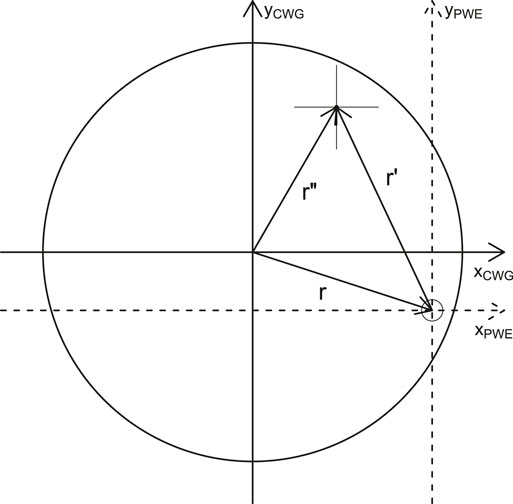
FIGURE 1. Cylindrical waveguide coordinate system (CWG). The natural coordinate system of the waveguide is rʺ and a point r at which we perform a partial wave expansion (PWE) in vector spherical wave functions (VSWF). In the new system, the expansion is done in the rʹ coordinate system, the fields are described by the Hansen multipoles and the GTE/TM coefficients, that are constant in the rʹ frame, but varies depending on the position of the expansion r.
4 Cylindrical Waveguide BSC’s
Using Eqs 24, 25 and 32 of Ref. [24] the explicit expression for the BSCs for any mode of the waveguide is given by:
Here, our notation is that superscript TE/TM means the spherical Transverse Electric/Magnetic in the sphere, while (TE)/(TM) means the waveguide TE/TM modes,
5 Optical Forces
In a recent review, it was demonstrated how optical forces can be derived from the Maxwell stress tensor given the BSCs in the Minkowski formalism [28]. Explicitly, in Eq. 93 in Ref. [28] provides the expression for the transverse forces, while the force in the z–direction is given by Eq. 94 in Ref. [28]:
where
From the expression of z-component of the force we substitute the BSCs expressions into the force equation, and using the normalization for the force
We display the equation in this way to demonstrate that all particle properties, such as size and refractive index, are embedded in the Mie factors Ap, Bp and Cp. Breaking the q sum into q = 0, q > 0 and q < 0, and using
The [radial, azimuthal] forces can be written in the same way:
While these equations could be written in a more compact way, we want to highlight the dependence of the real and imaginary parts of the Mie factors Ap, Bp and Cp, because these factors define the Mie resonances, as well as their scaling with particle size and relative refraction index, which are important to the sorting process. The dependence of the position of the particle inside the waveguide is embedded in the form factors
It becomes immediately clear that Fz depends on the real part of Ap, Bp and Cp only. In principle,
These expressions are general and can be used to obtain the force for any waveguide mode and particle size. Special care must be taken in the choice of highest p to truncate the series. The Wiscombe criterion was to truncate the sum when
In the following sections we will discuss two special cases. The first is related to use of the optical chromatography (OC) for nanoparticles that are well in the Rayleigh limit
The second case is waveguide-based OC for microparticles, such as dielectric spheres or virus–loaded droplets, with sizes in the Mie regime
6 Mie Coefficients in Rayleigh Regime
We can use the series expansion of spherical Bessel and Hankel function keeping the lowest orders of the imaginary and real parts to obtain [31]:
For the lowest terms we obtain
Reports on the scattering of metallic nanoparticles usually call the lowest terms approximations as modified long–wavelength approximation [32–35]. We shall not neglect the second term because they are real while the first are imaginary. Except for TE[m = 0] modes, we will keep only terms with
Without absorption, the leading term comes only from a1, and only A1 = a1 and C1 = a1 shall be considered. The only
In the expressions for the force, we get
for the z-component and
for the radial component, while the azimuthal one is given by
Next the form factors are calculated. We can bring all of them in terms of Jm(x) instead of
in the three line one column notation for the form factors. The TM case is then written as
This means that
which is proportional to particle radius to the sixth power and to the wavelength to the inverse forth power, as expected int he Rayleigh regime. The radial force in Rayleigh regime is given by
and
Therefore, the radial force
is proportional to the particle’s radius to the third power. The maximum radial force exceeds the axial scattering force, and keeps the particle near the position of maximum of the field intensity. Although some waveguide modes a zero intensity on axis, the commonly excited fundamental waveguide mode does tend to bring particles back to it's center. Finally, we discuss the azimuthal force. This force has two terms, one proportional to
that shows a gradient force type for the transverse force, and scattering force type for the axial force,
7 Forces Acting on-Axis Particles
For on-axis Mie-particles,
which cancels the sum in q, and
Clearly the sin form is null for m = 0 and cos form is just half of ±. The result ± form is
For the first modes where
which are nonzero only for the m = 0 and m = 1 modes. Also, for m = 0 modes the force for any particle size simplifies to:
On axis force in the Rayleigh regime can be obtained by making p = 1,
8 Results
We analyzed the important role of Mie Resonances, for different refractive index particles as a function of their sizes. Typical glass particles and liquid droplets have refractive indices in the range between 1.3 and 1.5, but semiconductors can have n as high as 3. Usually the high refractive index appears at the absorption band edge, except for quantum dots (QD), for which the optical gap is larger than the bulk band gap. Although QD are typically smaller than 10 nm sizes, one could also consider highly QD–doped microparticles with optical properties that are dominated by the QD refractive index. Therefore, in this analysis, we considered two limits of 1.3 and 3.0 for the refractive index. To exemplify this, the axial force for TE10 and TM10 modes was calculated as a function of particle radius for a n = 1.3 and n = 3.0 refractive index, assuming a air-filled waveguide with a diameter of
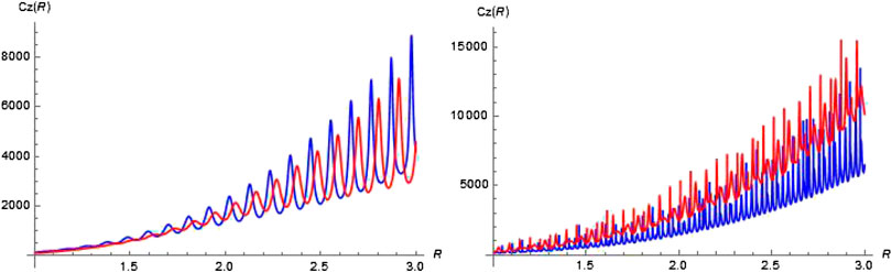
FIGURE 2. Axial force for: left n = 1.3 particle; right n = 3 particle. Blue TE10 mode, red TM10 mode of a 10 μm radius cylindrical waveguide.
For both particles, the resonances becoming narrower as the radius increases, with the narrowest resonances occurring for the n = 3 particle. The optical force landscape of the two particle’s parameters, size and relative refractive index is shown in map plot in Figure 3. The results suggest that Mie resonances can indeed be used to discriminate between a narrow range of discrete particles.
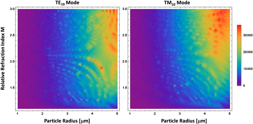
FIGURE 3. Density plot of axial force as function of particle’s relative refractive index M and particle radius for a 10 μm radius cylindrical waveguide.
Figures 4 and 5 show the forces for the first four first TE and TM modes for a Rayleigh particle inside a cylindrical waveguide. The axial force Fz is clearly proportional to the local field intensity
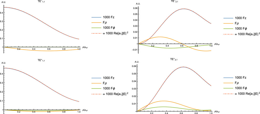
FIGURE 4. First TE modes: optical forces seen as profile from the center to the walls of the waveguide. Depending on the mode
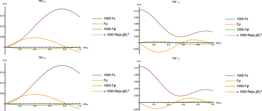
FIGURE 5. First TM modes: optical forces seen as profile from the center to the walls of the waveguide. As we have the
In the above calculation, we have used the full expressions for the force calculation. We used a wavelength of
Figure 6 shows how the force varies with size parameter (and in this case is directly proportional to the size of the particle x = ka). It also shows the truncation criteria for calculating these forces. In this case, the forces are of the same magnitude (we are far from the Rayleigh regime). There are some challenges to use this methodology to perform particle sorting. The first is how to load the particles into the waveguide, to start the sorting process.
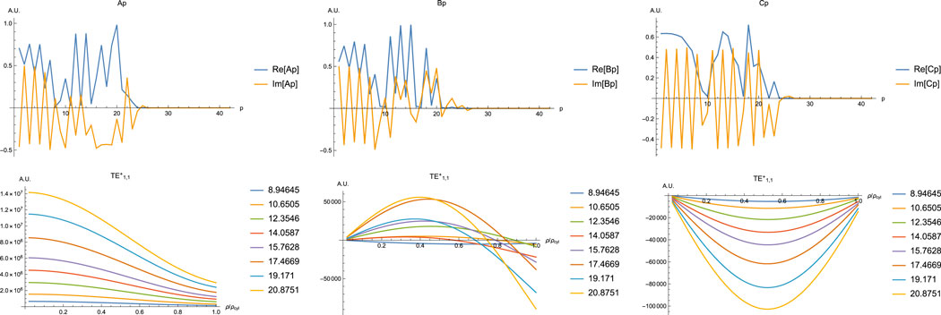
FIGURE 6. At the top the coefficients for x = 20.8751 (for a particle of 3.5 µm and a refractive index of 3. At bottom the forces (from left right Fz,
9 Conclusion and Discussion
We have demonstrated analytical expressions for optical forces acting on particles inside cylindrical waveguides. The theory is valid for particle radius a ranging from the Rayleigh regime to large microparticles, and for arbitrary particle position and optical modes. Analytical results obtained for a range of different particles sizes and refractive indices demonstrate that Mie-resonances can result in a strong size-dependence of the scattering force, with implications for waveguide-based particle sorting. In the Rayleigh regime, the radial, axial, and azimuthal forces were studied as a function of particle position within the waveguide. In the Rayleigh regime, the most important factor for particles sorting is found to be the x3, x6 size scale of the optical forces, followed by the refractive index differences, and the presence of absorption.
A possible application of this work would be post–synthesis size selection of quantum dots. Quantum dots are nanoparticles in the 1–10 nm diameter sizes, well in the Rayleigh regime, which show a size dependent optical band gap. We have produced quantum dots by chemical synthesis and, also, by Pulsed Laser Deposition (PLD) [36–38]. The advantage of PLD is a total degree of freedom regarding the material, just by focusing a powerful laser beam on any piece of solid bulk material, to produce a broad range of nano/micro-particles. It can be used with radioactive materials, semiconductors, or oxides, which can be hard to produce by chemical synthesis. PLD, however, produces a much wider size distribution than the chemical synthesis methods. Hence, the possibility to sort the quantum dots can make this technique more attractive, especially inside a waveguide where no particles are lost and that can be reprocessed. For this application, one can use the size–dependent absorption edges. With a tunable laser one can start with the longer wavelengths for which only the largest QDs absorb. Because the force in the presence of absorption scales with x3, much larger than the x6 non-absorbing QDs, one can isolate biggest absorbing QDs. The wavelength of the laser can then be swept, from the long to short, to perform an absorption–selective size separation. QDs usually have cap layers that change their hydrodynamic radii and their diffusion times in a liquid medium [39]. It would therefore also be possible to QDs of equal semiconductor core radius, through their cap layer thickness.
Furthermore, for microparticles (
For solid particles, we suggest to follow the particle–loading process used by [20], which mechanically removes the particles from a glass plate, and uses two counter-propagation beams to confine them to a region in front of the waveguide entrance. To launch a particles, the counter propagating beam is switched off and the particle is optically guided through the waveguide. The collection and sorting at the end of the waveguide can be done by applying a sweeping transverse force to the particles the end of the waveguide, that directs the articles to a specific region on the collector - analogous to a mass spectrometer. There are a range of parameters that can be adjusted for optimal sorting performance, including wavelength, polarization, and optical power, all of which can be changed fast. In case of charges particles, commonly found in colloids and cells, transverse electric fields could be applied to the waveguide [40] to selectively collect or slow down particles based on their charge.
Experimentally available hollow waveguides are typically based on hollow-core photonic crystal fibers, for which the theory described here offers a reasonable approximation but no analytical expression. It will therefore be interesting to explore different ways to create small-diameter cylindrical hollow metallic waveguides. One approach could be based on coating metal on the interior of a tube of a material with a thermal softening point close to that of the metal and subsequently draw this to optical fiber. Before the drawing, some propagation modes could be suppressed by laser cutting the metal perpendicular to the wall’s currents of the targeted modes.
Data Availability Statement
The raw data supporting the conclusions of this article will be made available by the authors, without undue reservation.
Author Contributions
CC, TE, and AN started the development of the theory, never published before, back in 2008 in Max Planck Institute in Erlangen, Germany, and conceived the idea for this report. WM developed the Fourier Transform method to calculate the BSCs. AF and AN performed the calculations of Mie resonances on optical forces. All the authors wrote, edited, reviewed and revised the manuscript. CC supervised the study.
Conflict of Interest
The authors declare that the research was conducted in the absence of any commercial or financial relationships that could be construed as a potential conflict of interest.
Acknowledgments
AF acknowledges the National Institute of Photonics (INFo). CC acknowledges National Institute of Science and Technology in Photonics Applied to Cell Biology [INFABIC] CNPq (573913/2008-00/FAPESP (08/57906-3); CNPq grant (312049/2014-5); “Física do Petróleo em Meios Porosos”, PETROBRAS-UFC (2016/00328-4) and F020/WIPPS II—Simulação numérica de invasão de água em poços produtores”, PETROGAL-UFC T.G.E. acknowledges the support from the Winton Program for the Physics of Sustainability, the Isaac Newton Trust, and the Leverhulme Trust (RPG‐2018‐256).
References
1. Ashkin A. Acceleration and trapping of particles by radiation pressure. Phys Rev Lett (1970) 24:156–9. doi:10.1103/PhysRevLett.24.156
2. Fontes A, Neves AAR, Moreira WL, de Thomaz AA, Barbosa LC, Cesar CL, et al. Double optical tweezers for ultrasensitive force spectroscopy in microsphere mie scattering. Appl Phys Lett (2005) 87:221109. doi:10.1063/1.2137896
3. Neves AAR, Fontes A, de Y Pozzo L, de Thomaz AA, Chillce E, Rodriguez E, et al. Electromagnetic forces for an arbitrary optical trapping of a spherical dielectric. Optic Express (2006) 14:13101–6. doi:10.1364/OE.14.013101
4. Rohrbach A. Switching and measuring a force of 25 femtonewtons with an optical trap. Optic Express (2005) 13:9695–701. doi:10.1364/OPEX.13.009695
5. Callegari A, Mijalkov M, Gököz AB, Volpe G. Computational toolbox for optical tweezers in geometrical optics. J Opt Soc Am B (2015) 32:B11–9. doi:10.1364/JOSAB.32.000B11
6. Jonáš A, Zemánek P. Light at work: the use of optical forces for particle manipulation, sorting, and analysis. Electrophoresis (2008) 29:4813–51. doi:10.1002/elps.200800484 |
7. Fontes A, Fernandes HP, de Thomaz AA, Barbosa LC, Barjas-Castro ML, Cesar CL. Measuring electrical and mechanical properties of red blood cells with double optical tweezers. J Biomed Optic (2008) 13:1–6. doi:10.1117/1.2870108
8. Fontes A, Ajito K, Neves AAR, Moreira WL, de Thomaz AA, Barbosa LC, et al. Raman, hyper-Raman, hyper-Rayleigh, two-photon luminescence and morphology-dependent resonance modes in a single optical tweezers system. Phys Rev (2005b) 72:012903. doi:10.1103/PhysRevE.72.012903 |
9. Chu S, Bjorkholm JE, Ashkin A, Cable A. Experimental observation of optically trapped atoms. Phys Rev Lett (1986) 57:314–7. doi:10.1103/PhysRevLett.57.314 |
10. Imasaka T, Kawabata Y, Kaneta T, Ishidzu Y. Optical chromatography. Anal Chem (1995) 67:1763–5. doi:10.1021/ac00107a003
11. Hatano T, Kaneta T, Imasaka T. Application of optical chromatography to immunoassay. Anal Chem (1997) 69:2711–5. doi:10.1021/ac970081q |
12. Hart SJ, Terray AV. Refractive-index-driven separation of colloidal polymer particles using optical chromatography. Appl Phys Lett (2003) 83:5316–8. doi:10.1063/1.1635984
13. Terray A, Arnold J, Hart SJ. Enhanced optical chromatography in a pdms microfluidic system. Optic Express (2005) 13:10406–15. doi:10.1364/OPEX.13.010406
14. Hart SJ, Terray A, Arnold J, Leski TA. Sample concentration using optical chromatography. Optic Express (2007) 15:2724–31. doi:10.1364/OE.15.002724 |
15. Terray A, Hebert CG, Hart SJ. Optical chromatographic sample separation of hydrodynamically focused mixtures. Biomicrofluidics (2014) 8:064102. doi:10.1063/1.4901824 |
16. Kaneta T, Ishidzu Y, Mishima N, Imasaka T. Theory of optical chromatography. Anal Chem (1997) 69:2701–10. doi:10.1021/ac970079z |
17. Euser TG, Garbos MK, Chen JSY, Russell PS. Precise balancing of viscous and radiation forces on a particle in liquid-filled photonic bandgap fiber. Opt Lett (2009) 34:3674–6. doi:10.1364/OL.34.003674 |
18. Marcatili EAJ, Schmeltzer RA. Hollow metallic and dielectric waveguides for long distance optical transmission and lasers. Bell Syst Tech J (1964) 43:1783–809. doi:10.1002/j.1538-7305.1964.tb04108.x
19. Garbos MK, Euser TG, Schmidt OA, Unterkofler S, Russell PS. Doppler velocimetry on microparticles trapped and propelled by laser light in liquid-filled photonic crystal fiber. Opt Lett (2011) 36:2020–2. doi:10.1364/OL.36.002020 |
20. Schmidt OA, Garbos MK, Euser TG, Russell PSJ. Metrology of laser-guided particles in air-filled hollow-core photonic crystal fiber. Opt Lett (2012) 37:91–3. doi:10.1364/OL.37.000091 |
21. Sharma A, Xie S, Zeltner R, Russell PS. On-the-fly particle metrology in hollow-core photonic crystal fibre. Optic Express (2019) 27:34496–504. doi:10.1364/OE.27.034496
22. Mie G. Beiträge zur optik trüber medien, speziell kolloidaler metallösungen. Ann Phys (1908) 330:377–445.
23. Moreira WL, Neves AAR, Garbos MK, Euser TG, Russell PSJ, Cesar CL. Expansion of arbitrary electromagnetic fields in terms of vector spherical wave functions (2010). e-printsArXiv: 1003.2392.
24. Moreira WL, Neves AAR, Garbos MK, Euser TG, Cesar CL. Expansion of arbitrary electromagnetic fields in terms of vector spherical wave functions. Optic Express (2016) 24:2370–82. doi:10.1364/OE.24.002370
25. Mangini F, Tedeschi N. Scattering of an electromagnetic plane wave by a sphere embedded in a cylinder. J Opt Soc Am A (2017) 34:760–9. doi:10.1364/JOSAA.34.000760
28. Neves AAR, Cesar CL. Analytical calculation of optical forces on spherical particles in optical tweezers: tutorial. J Opt Soc Am B (2019) 36:1525–37. doi:10.1364/JOSAB.36.001525
29. Wiscombe WJ. Improved mie scattering algorithms. Appl Optic (1980) 19:1505–9. doi:10.1364/AO.19.001505
30. Neves AAR, Pisignano D. Effect of finite terms on the truncation error of mie series. Opt Lett (2012) 37:2418–20. doi:10.1364/OL.37.002418 |
31. Bohren C, Huffman D. Absorption and scattering of light by small particles. Weinheim, Germany: Wiley (1983).
32. Kuwata H, Tamaru H, Esumi K, Miyano K. Resonant light scattering from metal nanoparticles: practical analysis beyond Rayleigh approximation. Appl Phys Lett (2003) 83:4625–7. doi:10.1063/1.1630351
33. Schebarchov D, Auguié B, Le Ru EC. Simple accurate approximations for the optical properties of metallic nanospheres and nanoshells. Phys Chem Chem Phys (2013) 15:4233–42. doi:10.1039/C3CP44124E |
34. Moroz A. Depolarization field of spheroidal particles. J Opt Soc Am B (2009) 26:517–27. doi:10.1364/JOSAB.26.000517
35. Kelly KL, Coronado E, Zhao LL, Schatz GC. The optical properties of metal nanoparticles: the influence of size, shape, and dielectric environment. J Phys Chem B (2003) 107:668–77. doi:10.1021/jp026731y
36. González-Castillo JR, Rodriguez E, Jimenez-Villar E, Rodríguez D, Salomon-García I, de Sá GF, et al. Synthesis of ag@silica nanoparticles by assisted laser ablation. Nanoscale Research Letters (2015) 10:399. doi:10.1186/s11671-015-1105-y |
37. Ermakov VA, Jimenez-Villar E, Silva Filho JMC, Yassitepe E, Mogili NVV, Iikawa F, et al. Size control of silver-core/silica-shell nanoparticles fabricated by laser-ablation-assisted chemical reduction. Langmuir (2017) 33:2257–62. doi:10.1021/acs.langmuir.6b04308 |
38. González-Castillo JR, Rodríguez-González E, Jiménez-Villar E, Cesar CL, Andrade-Arvizu JA. Assisted laser ablation: silver/gold nanostructures coated with silica. Appl Nanosci (2017) 7:597–605. doi:10.1007/s13204-017-0599-2
39. Pereira MIA, Pereira G, Monteiro CAP, Geraldes CFGC, Cabral Filho PE, Cesar CL, et al. Hydrophilic quantum dots functionalized with gd(iii)-do3a monoamide chelates as bright and effective t1-weighted bimodal nanoprobes. Sci Rep (2019) 9:2341. doi:10.1038/s41598-019-38772-8 |
Keywords: optical forces, optical trapping, waveguides, Scattering theory, optical chromatography
Citation: Neves AAR, Moreira WL, Fontes A, Euser TG and Cesar CL (2021) Toward Waveguide-Based Optical Chromatography. Front. Phys. 8:603641. doi: 10.3389/fphy.2020.603641
Received: 07 September 2020; Accepted: 07 December 2020;
Published: 10 February 2021.
Edited by:
Halina Rubinsztein-Dunlop, The University of Queensland, AustraliaReviewed by:
Weiqiang Ding, Harbin Institute of Technology, ChinaIlia L. Rasskazov, University of Rochester, United States
Copyright © 2021 Neves, Moreira, Fontes, Euser and Cesar. This is an open-access article distributed under the terms of the Creative Commons Attribution License (CC BY). The use, distribution or reproduction in other forums is permitted, provided the original author(s) and the copyright owner(s) are credited and that the original publication in this journal is cited, in accordance with accepted academic practice. No use, distribution or reproduction is permitted which does not comply with these terms.
*Correspondence: Carlos L. Cesar, lenz@ifi.unicamp.br