Test model coverage analysis under uncertainty: extended version

Prasetya, I. S. W. B.; Klomp, Rick

doi:10.1007/s10270-020-00848-9

Test model coverage analysis under uncertainty: extended version

Special Section Paper
Open access
Published: 09 February 2021

Volume 20, pages 383–403, (2021)
Cite this article

Download PDF

You have full access to this open access article

Software and Systems Modeling Aims and scope Submit manuscript

Test model coverage analysis under uncertainty: extended version

Download PDF

1308 Accesses
1 Citation
1 Altmetric
Explore all metrics

Abstract

In model-based testing, we may have to deal with a non-deterministic model, e.g. because abstraction was applied, or because the software under test itself is non-deterministic. The same test case may then trigger multiple possible execution paths, depending on some internal decisions made by the software. Consequently, performing precise test analyses, e.g. to calculate the test coverage, are not possible.. This can be mitigated if developers can annotate the model with estimated probabilities for taking each transition. A probabilistic model checking algorithm can subsequently be used to do simple probabilistic coverage analysis. However, in practice developers often want to know what the achieved aggregate coverage is, which unfortunately cannot be re-expressed as a standard model checking problem. This paper presents an extension to allow efficient calculation of probabilistic aggregate coverage, and also of probabilistic aggregate coverage in combination with k-wise coverage.

A systematic review of fuzzing

Article 31 October 2023

Introduction to Model Checking

The probabilistic model checker Storm

Article Open access 06 July 2021

1 Introduction

Model-based testing (MBT) is considered as one of the leading technologies for systematic testing of software [4, 6, 26]. It has been used to test different kinds of software, e.g. communication protocols, web applications, and automotive control systems. In this approach, a model describing the intended behaviour of the system under test (SUT) is first constructed [37], and then used to guide the tester, or a testing algorithm, to systematically explore and test the SUT’s states. Various automated MBT tools are available, e.g. JTorX [3, 33], Phact [14], OSMO [23], APSL [34], and RT-Tester [26].

There are situations where we end up with a non-deterministic model [19, 26, 31], for example when the non-determinism within the system under test, e.g. due to internal concurrency, interactions with an uncontrollable environment (e.g. as in cyber physical systems), or use of AI, leads to effects observable at the model level. Non-determinism can also be introduced as by-product when we apply abstraction on an otherwise too large model [28]. Models mined from execution logs [10, 30, 38] can also be non-deterministic, because log files only provide very limited information about system’s states. (Hence, we essentially apply an abstraction).

MBT with a non-deterministic model is more challenging. The tester cannot fully control how the SUT would traverse the model, and cannot thus precisely determine the current state of the SUT. Obviously, this makes the task of deciding which trigger to send next to the SUT harder. Additionally, coverage, e.g. in terms of which states in the model have been visited by a series of tests, cannot be determined with 100% certainty either. This paper will focus on addressing the latter problem—readers interested in test cases generation from non-deterministic models are referred to, e.g. [19, 24, 36]. Rather than simply stating that a test sequence may cover some given state, to be more helpful we propose to calculate the probability of covering a given coverage goal, given modelers’ estimation on the local probability of each non-deterministic choice in a model.

Given a probabilistic model of the SUT, e.g. in the form of a Markov Decision Process (MDP) [5, 32], and a test $\sigma $ in the form of a sequence of interactions on the SUT, the most elementary type of coverage goal in MBT is for $\sigma $ to cover some given state s of interest in the model. Calculating the probability that this actually happens is an instance of the probabilistic reachability problem which can be answered using, e.g. a probabilistic model checker [5, 9, 16, 21]. However, in practice coverage goals are typically formulated in an ‘aggregate’ form, e.g. to cover at least 80% of the states, without being selective on which states to include. Additionally, we may want to know the aggregate coverage over pairs of states (the transitions in the model), or vectors of states, as in k-wise coverage [1]. This is of practical interest as different research showed that k-wise significantly increases the fault finding potential of a test suite [11, 25]. Aggregate goals cannot, however, be expressed in LTL or CTL, which are the typical formalisms in model checking, and therefore we cannot use a model checker to analyse them either. Furthermore, both types of goals (aggregate and k-wise) may lead to combinatorial explosion.

This paper is an extended version of [27] that was presented at the 17th International Conference on Software Engineering and Formal Methods (SEFM) in 2019; they contribute the following:

1.
A concept and definition of probabilistic test coverage; as far as we know this has not been covered in the literature before. To formalise the concept, a minimalistic language is introduced to express coverage goals. The language is partly a susbet of CTL, but also extends the latter with aggregate formulas.
2.
An algorithm to calculate probabilistic coverage, in particular of aggregate k-wise coverage goals.

With respect to [27] this paper includes a new subsection on calculating the probabilistic coverage at the test suite level and a new subsection that formalises the concept of probabilistic ‘coverage metrics’ and how to calculate them. We also include some new results on using different merging policies when calculating probabilistic aggregate coverage and a new experiment where we evaluate our algorithm on a model of the backoff mechanism of the IEEE 802.11 WLAN protocol.

Paper structure Section 2 contains preliminaries to introduce various formal models that we will need to present out theory. Section 3 introduces the needed testing-related concepts such as what a test case is and what probabilistic coverage means. We also introduce the concept of execution model, which is a key concept for our algorithm. Section 4 introduces the kind of coverage goals we want to be able to express and how their probabilistic coverage can be calculated. Section 5 presents our algorithm for efficient coverage calculation. Section 6 discusses two experiments to benchmark our algorithm and shows the results. Related work is discussed in Sect. 7. Section 8 concludes.

2 Preliminaries: notation and formal models

In this section, we will introduce different kinds of formal models of systems, along with some general notations, that this paper will need to present its theory. Three kinds of models will be needed: Labelled Transition System (LTS), Markov Decision Process (MDP) and Markov Chain. LTS is commonly used in Model-Based Testing. MDP is a probabilistic extension of LTS and Markov Chain is a special instance of MDP.

2.1 General notation

A sequence of items will be denoted by either abc or a, b, c. An empty sequence is denoted by $\epsilon $. If $\sigma _1$ and $\sigma _2$ are sequences, $\sigma _1 \sigma _2$ denotes the sequence obtained by concatenating them. If $\sigma $ is a sequence, its $i^{\mathrm{th}}$-element is denoted by $\sigma _i$; the counting starts from 0. We also write $\mathsf{tail}(\sigma )$ to refer to the rest of $\sigma $ beyond $\sigma _0$.

When u is some entity (e.g. it could be a node in a graph), we may need to introduce some additional attributes for u, e.g. “st” or “lab”. To improve readability, we usually denote them in the dot-style as in: $u.\mathsf{st}$ and $u.\mathsf{lab}$. The notation is more suggestive in indicating that, e.g. $\mathsf{st}$ is an attribute (as opposed to writing it as st(u)).

2.2 Labelled transition system

An intuitive and abstract way to model a system is by using a labelled transition system (LTS) [2]. Although our focus later will be on a probabilistic extension of LTS, let us first introduce some basic LTS concepts and notations as we will also use them when discussing probabilistic models.

An example is shown below: an LTS model called $\mathsf{EX}_0$, consisting of three states, with 0 as the starting state.

The arrows denote transitions between states, each is labelled by the action that causes the transition. For example, the arrow $0\; {\xrightarrow {\ b\ }}\; 1$ means that executing the action b when the system is in the state 0 ‘would’ cause it to move to the state 1; the precise definition is given below.

Actions like a and b represent an interaction between the system and its environment. Consequently actions are observable by the environment. We also call them ‘external’ (and later we will also introduce ‘internal action’).

In our set-up, the environment is a ‘tester’, which is a person or a computer program that tries to test the system. We will limit our scope to systems whose actions are synchronous a la CSP [18]. That is, for an action a to take place, both the system and the environment first need to agree (to synchornise) on doing a; then they will do a together. For example, the state 0 of the model $\mathsf{EX}_0$ above has two outgoing transitions labelled by a and b. The choice between these transitions is made together. So, the system cannot unilaterally just decide to do a without the environment agreeing on doing that.

Definition 1

Formally an LTS is a tuple $L = (S,s_0,$ $A,{\rightarrow })$ where S is a finite set of states, $s_0\in S$ is L’s initial state. A is a finite set of actions. The last element, $\rightarrow \subseteq S\times A \times S$ is relation describing the transitions: for any s and a, the set:

$$\begin{aligned} \{ \; t \; | \; s \xrightarrow {a} t \; \} \end{aligned}$$

specifies the set of all possible states that L will transition to when executing the action a on the state s.

The definition indeed only allows a single initial state. Multiple initial states can be modelled through $\tau $-transitions explained later.

Since we later often need to quantify over different elements of an LTS (e.g. quantifying over its states or over its executions), for convenience we will overload the $\in L$ notation:

If s is a state, $s {\in } L$ means that s is a state in L (so, $s\in S$).
$s \xrightarrow {a} t\in L$ means that $s \xrightarrow {a} t$ is a transition in L.
If $\rho $ is an execution (introduced later), $\rho \in M$ means that $\rho $ is a possible execution of M.

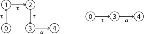
The definition of LTS allows us to have models that behave non-deterministically. A model is deterministic if for any sequence of external actions, executing the sequence on the model always lead to a unique state in the model. Otherwise, the model is non-deterministic. In the examples below, the model on the left is deterministic. The model on the right is non-deterministic, because executing a can lead to either the state 2 or the state 3.

The model $\mathsf{EX}_0$ shown before is also non-deterministic, as the set $\{ \; t \; | \; 0 \xrightarrow {a} t \; \} = \{ 1,2 \}$ is not a singleton. So, executing a on the state 0 can take the system to either the state 1 or the state 2. The choice is assumed to be made internally by the system, beyond the control of the environment/tester.

Ideally, a system’s internal transitions which are not visible to the environment should be abstracted away in its model. However, some of them might dynamically influence the set of visible actions that the system can do. For example, in the ‘system’ below, $\tau $ is an internal transition. In the state 0 this system can still do a, but if the internal transition $\tau $ happens, the system will move to the state 2, where a is no longer possible.

In such a case, it becomes necessary to also include internal transitions in the model. We will therefore allow L to contain a special $\tau $-action:

Definition 2

($\tau $-action and transition) $\tau $ represents a system’s internal action. A transition $s \xrightarrow {\tau } t$ can happen without requiring any synchornisation with the environment, and is also not visible to the environment.

Note that although a $\tau $-transition is not visible, the environment may still be able to infer that it was taken (or otherwise: that it was not taken) by observing the next visible actions. For example, if the environment of $L_0$ above observes a, then the $\tau $-transition to the state 2 could not have taken place.

Definition 3

(Execution) An execution of a system in terms of its model L is a finite path $\rho $ through L, starting from L’s initial state. We will write $\rho {\in } L$ to denote this. We will represent $\rho $ by a sequence of transitions such that: (1) if $s \xrightarrow {a} t$ is the first transition in $\rho $, then s should be the model’s initial state; (2) if $s \xrightarrow {a} t$ and $s' \xrightarrow {b} t'$ are two consecutive transitions in $\rho $, then $t{=}s'$.

Definition 4

(Trace) A trace is a finite sequence of observable (non-$\tau $) actions. If $\rho $ is an execution, the trace it induces will be denoted by $\mathsf{tr}(\rho )$.

Note that not all parts of an execution are observable by the environment. However, a trace is always observable.

Also notice that the presence of $\tau $-transitions introduce non-determinism. For example, in the example $L_0$, if the environment so far observes no action, the system could still be in the state 0, or it might already move to 2.

To later simplify calculation over non-deterministic transitions, we will require the modeller to have normalised the models by removing ‘unnecessary’ $\tau $-transitions. A model L is $\tau $-normalised if the following hold:

1.
A state cannot have a mix of $\tau $ and non-$\tau $ outgoing transitions. For example, a model such as $L_0$ (shown again below) is excluded from our consideration. Such a model implies that the system can either internally decide to synchronise on a, or to reject it. The model should be re-modelled to $L_1$ that equivalently captures this decision point by introducing an intermediate state 1a.
2.
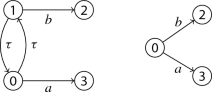
L should have no intermediate state (a state with at least one predecessor and at least one successor) whose all incoming and outgoing transitions are $\tau $ transitions. Such a state is not considered as interesting for our analyses. For example, states 1 and 2 in the left model below should removed. We should re-model it to the next model on the right.
3.
L should not contain a cycle that consists of only $\tau $ transitions. As an example, the left model below contains such a cycle. We should re-model it to the model on the right.

If $\rho $ and $\rho '$ are executions producing the same trace, one can be longer than the other. This is the case if one does more $\tau $-transitions than the other. An execution is called $\tau $-maximal if it cannot be extended further by inserting $\tau $-transitions (and still forms a valid execution). Models which are $\tau $-normalised have the following property: if we exclude executions which are not $\tau $-maximal, non-determinism can only be introduced if there is a state s where the same action (which can be $\tau $) can lead to multiple direct successor states. We will use this property later to simplify our analyses.

2.3 Markov process and chain

A Markov Decision Process (MDP) is a way to model a system that behaves stochastically. We can also see it as a refinement of LTS. Whereas in an LTS, when an action behaves non-deterministically all we can say is the set of possible states where it might end up with, with an MDP we can specify the probability of ending up in each of those states. The formal definition is below, which we adapt from [5].

Definition 5

A Markov Decision Process (MDP) $M = (S,s_0,A,\rightarrow ,P)$ is an LTS with P as an additional component, called probability function. For each transition $s \xrightarrow {a} t$, $P(s \xrightarrow {a} t)$ is an $\mathbb {R}$ value specifying the probability that the system will end in the state t, when a is executed on the state s. The sum of the probabilities should be 1. More precisely, the following should hold. For every $s\in S$ and $a\in A$:

$$\begin{aligned} \sum _{t \ s.t. \ s \xrightarrow {a} t} P(s \xrightarrow {a} t) \ \ = \ \ 1 \end{aligned}$$

For example, consider again the LTS $\mathsf{EX}_0$ from Sect. 2.2. We can refine this model by turning it to an MDP by annotating each transition with its probability. An example is shown below. The number between parentheses is the probability of the corresponding transition.

The MDP above specifies that executing a on the state 0 has a 0.5 probability to end in the state 1, and likewise for ending up in 2. Since these are the only two possible end states for a when executed on s, the sum of their probabilities should be 1^{Footnote 1}. Note that probability of, e.g. the transition $0 \xrightarrow {b} 1$ is necessarily 1.0, because 1 is the only possible end state when executing b on the state 0.

In the sequel, when a transition has a probability 1, we will remove its probability annotation from the model.

Notice that in an MDP there can be multiple actions that can be executed on a given state, e.g. in the above example actions a and b are both possible when the system is in the state 0. The decision to choose between them is deterministic. Only the choice between outgoing transitions with the same label is non-deterministic. A special case is the following, called Markov Chain:

Definition 6

A Markov Chain is an MDP M where at every $s\in M$ there is at most one action possible. So, the set $\{ \alpha \; | \; s \xrightarrow {\alpha } t \in M \}$ has at most one element.

In other words, every state in a Markov Chain has outgoing transitions that share the same action-label. We should note that in the literature, e.g. [5], this action label is typically removed (it is fully determined by the source state of the corresponding transition).

Below is an example of a Markov Chain.

The Markov Chain above is actually obtained by ‘unfolding’ the MDP $\mathsf{EX}_0$ given earlier, along all possible executions that produce the trace bba. Later, we will use Markov Chain to model the set of possible executions of a test case (whereas Markov Decision Process/MDP is used to model the system that we test).

3 Test case, test suite, and simple coverage

We can now turn our attention to testing. As a running example, consider the labelled transition system (LTS) in Fig. 1 as a model of some system under test (SUT). The system interacts with its environment through actions a, b, and c. These actions are thus external and observable by the environment. The model also includes several $\tau $-transitions. These are internal transitions. The model is also $\tau $-normalised. As can be seen, the model is non-deterministic. For example, the action a at the initial state 0 is non-deterministic with $\{1,2\}$ as the possible end states.

To test the SUT, the tester takes the role of the environment. It tries to control the SUT by interacting with it, and then observing if the SUT behaves as expected. Recall that in our setup actions such as a and b represent interactions between the SUT and the environment. Furthermore, actions are assumed to be synchronous. So, to control the SUT the tester would insist on doing a certain action of its choice. For example, if on the state t the SUT is supposed to be able to either do a or b, the tester can insist on doing a. If the SUT fails to go along with this, it is an error. The tester can also test if in this state the SUT can be coerced to do an action that it is not supposed to synchronise; if so, the SUT is incorrect.

We will assume a black box setup. That is, the tester cannot actually see the SUT’s state, though the tester can try to infer this based on information visible to him/her, e.g. the trace of the external actions done so far. For example, after doing a from the state 0 on the SUT $\mathsf{EX}_1$ above, the tester cannot tell whether it then goes to the state 1 or 2. However, if the tester manages to do abc he/she would on the hindsight know that the state after a must have been 1. Such hindsight reasoning does not always eliminate all uncertainty though. For example, after doing aba the tester will not be able tell for certain whether or not the test ends at the state 1 and covers the state 4 along the way. We can indeed still say, e.g. that the end state must be one of $\{1,2\}$, but that is as far as what we can infer given the information we have in the model. However, if we had an MDP model instead of a plain LTS, we would then be able to tell what the probability is of ending in either of the states. The tester can then make a better informed decision, e.g. to repeat the test to improve the probability of covering a certain state, or to come up with a new test.

To provide a more refined test analysis let us now assume that the modeller is able to estimate the probability of taking each of the non-deterministic transitions in the LTS model and annotate this on each of them. Such estimation can be derived for example from the description of the algorithm that the system implements, e.g. when the algorithm prescribes that certain choices are to be taken randomly based on some given distribution. Non-determinism can also come from sources like concurrency whose distribution is hard to determine upfront. In such a case, runtime data can be collected and analysed, e.g. using procedures as in process mining, and then used as a base for such estimation [20].

Annotating an LTS model with probability information essentially turns it into an MDP. Imagine that for our running example, this results in the MDP model in Fig. 2.

In our theory, we will consider test cases abstractly: a test case is modeled by a trace. We will restrict to test cases that form ‘legal’ traces^{Footnote 2}. A legal trace is a trace that can actually be produced by some execution of the SUT. For example, ab, aba and ababc are legal traces, and hence also test cases for $\mathsf{EX}_1$ in Fig. 2. A set of test cases is also called a test suite.

Since the model can be non-deterministic, the same test case may trigger multiple possible executions which are indistinguishable from their trace. To denote them we introduce the following:

Definition 7

Let L be an LTS. If $\sigma $ is a trace over L’s actions, $\mathsf{exec}(\sigma )$ denotes the set of all executions $\rho $ of L such that $\mathsf{tr}(\rho ) {=} \sigma $, and moreover is $\tau $-maximal: it cannot be extended without breaking the property $\mathsf{tr}(\rho ) {=} \sigma $.

Note that an MDP is also an LTS, so the above definition also applies for MDPs. Insisting on $\tau $-maximality means that we will only consider executions that have executed all $\tau $-transitions that can possibly be executed (to produce the same trace). This will allow us to avoid having to reason about the possibility that $\rho $, after being observed as $\sigma $, is delayed in completing its final $\tau $ transitions. This information cannot be inferred from an MDP model.

3.1 Representing a test case as an ‘execution model’

In the sequel, let M be a $\tau $-normalised MDP model describing some SUT. The probability that a test case $\sigma $ covers some goal $\phi $ (e.g. a particular state s) can in principle be calculated by quantifying over $\mathsf{exec}(\sigma )$. However, if M is highly non-deterministic, the size of $\mathsf{exec}(\sigma )$ can be exponential with respect to the length of $\sigma $. To facilitate more efficient coverage calculation we will represent $\sigma $ with the (finite) subgraph of unrolled M that $\sigma $ induces. We will call this subgraph the execution model of $\sigma $, denoted by $\mathsf{E}(\sigma )$. For example, the execution model of the test case aba on $\mathsf{EX}_1$ is shown in Fig. 3. An artificial state denoted with $\sharp $ is added so that $\mathsf{E}(\sigma )$ has a single exit node, which is convenient for later.

$\mathsf{E}(\sigma )$ forms a Markov Chain; each branch in $\mathsf{E}(\sigma )$ is annotated with the probability of taking the branch, under the premise that $\sigma $ has been observed. Since a test case is always of finite length and M is assumed to have no $\tau $-cycle, $\mathsf{E}(\sigma )$ is always acyclic. Typically the size of $\mathsf{E}(\sigma )$, in terms of its number of nodes, is much less than the size of $\mathsf{exec}(\sigma )$.

To identify the states in $\mathsf{E}(\sigma )$ we assign fresh names to them ($u_0 \ldots u_8$ in Fig. 3). Introducing fresh names is necessary as $\mathsf{E}(\sigma )$ is obtained by unrolling M, so it may have more states than M itself. We write $u.\mathsf{st}$ to denote u’s state label, which is the state in M that u represents (so, $u.\mathsf{st} \in M$); in Fig. 3, this is denoted by the number between parentheses in every node.

Importantly, the probability of the transitions in $\mathsf{E}(\sigma )$ may be different than the original probability in M. For example, the transition $u_3 \xrightarrow {\tau } u_5$ in the execution model in Fig. 3 has probability 1.0, whereas in the original model $\mathsf{EX}_1$, this corresponds to the transition $3 \xrightarrow {\tau } 4$ whose probability is 0.9. This is because the alternative $3 \xrightarrow {\tau } 5$ could not have taken place, as it leads to an execution whose trace does not correspond to the test case aba (which is assumed to have happened).

More precisely, when an execution in the model $\mathsf{E}(\sigma )$ reaches a node u, the probability of extending this execution with the transition $u \xrightarrow {\alpha } v$ can be calculated by taking the conditional probability of the corresponding transition in the model M, given that only the outgoing transitions specified by $\mathsf{E}(\sigma )$ could happen. This probability is $P_M(u.\mathsf{st} \xrightarrow {\alpha } v.\mathsf{st})$ divided by the sum of $P_M(u.\mathsf{st} \xrightarrow {\alpha } w.\mathsf{st})$ of all w such that $u \xrightarrow {\alpha } w \in \mathsf{E}(\sigma )$.

Definition 8

Given a trace $\sigma \in M$ and its execution model $\mathsf{E}(\sigma )$, we write $P_{\mathsf{E}(\sigma )}(u \xrightarrow {\alpha } v)$ to denote the probability that $\mathsf{E}(\sigma )$ will take the transition when it is in the state u. This probability is calculated from M as follows:

$$\begin{aligned} \frac{P_M(u.\mathsf{st} \xrightarrow {\alpha } v.\mathsf{st})}{ \sum _{w \ \text{ s.t. } \ u \xrightarrow {\alpha } w \in \mathsf{E}(\sigma )} P_M(u.\mathsf{st} \xrightarrow {\alpha } w.\mathsf{st}) } \end{aligned}$$

Note that technically an ‘execution’ or a path $\rho $ of $\mathsf{E}(\sigma )$, due to the way we have defined what a model-execution constitutes, is a sequence over $\mathsf{E}(\sigma )$’s nodes rather than a sequence over M’s states, though the intention is of course to describe the latter. Let us then use this notation:

$$\begin{aligned} \mathsf{states}(\rho ) \end{aligned}$$

to denote the sequence of M’s states that $\rho $ represents. For example, the sequence $\rho = u_0 \xrightarrow {a} u_1 , u_1 \xrightarrow {b} u_4$ is an execution of the execution model in Fig. 3. Its $\mathsf{states}(\rho )$ is the sequence $u_0.\mathsf{st }, u_1.\mathsf{st } , u_4.\mathsf{st } = 0,1,0$.

Let $\rho $ be a full path/execution in $\mathsf{E}(\sigma )$ (a path from its initial to final node). Since $\mathsf{E}(\sigma )$ is acyclic, the probability that it traverses $\rho $ can be obtained by simply multiplying the probability of all the transitions in the path:

$$\begin{aligned} P_{\mathsf{E}(\sigma )}(\rho ) \ = \ \prod _{u \xrightarrow {\alpha } v \in \rho } P_{\mathsf{E}(\sigma )}(u \xrightarrow {\alpha } v) \end{aligned}$$

(1)

3.2 Example: simple coverage analyses

As an example of a simple analysis, let us calculate the probability that a test case $\sigma $ produces an execution that passes through a given state s. Let us denote this probability by:

$$\begin{aligned} P(\langle s \rangle \; | \;\sigma ) \end{aligned}$$

This probability would just be the sum of the probabilities of all full paths in $\mathsf{E}(\sigma )$ that contain s. So:

$$\begin{aligned} P(\langle s \rangle \; | \;\sigma ) \ = \ \sum _{\rho \; \text{ s.t. }\; \rho \in \mathsf{E}(\sigma ) \wedge s\in \mathsf{states}(\rho )} P_{\mathsf{E}(\sigma )}(\rho ) \end{aligned}$$

(2)

For example, below are the probabilities that the test case aba on $\mathsf{EX}_1$ would cover certain states. The probabilities are calculated through its execution model in Fig. 3.

State to cover	Probability
$P(\langle 0 \rangle \; \| \;aba)$	= 1.0
$P(\langle 1 \rangle \; \| \;aba)$	= 0.525
$P(\langle 2 \rangle \; \| \;aba)$	= 0.725
$P(\langle 3 \rangle \; \| \;aba)$	= 0.05
$P(\langle 4 \rangle \; \| \;aba)$	= 0.05
$P(\langle 5 \rangle \; \| \;aba)$	= 0

4 Coverage under uncertainty

Test coverage, or simply ‘coverage’, is an indicator for the completeness of a test suite. In practice, this is often expressed in terms of percentage, e.g. we may want to require that the test suite should have at least $p\%$ state coverage. Achieving higher p is taken as an indicator of having a more complete test suite^{Footnote 3}. Additionally, for the testers it is also important to know which states exactly are left uncovered so that they can figure out which test cases need to be added. In the probabilistic setup things become more complicated. We no longer can say for certain whether a state is covered or not, which further complicates the calculation of a test suite’s aggregate coverage.

Let us first introduce a language for expressing ‘coverage goals’; we will keep it simple, but expressive enough to express what is later called ‘aggregate k-wise’ goals. A coverage goal is a predicate on a test case or a test suite. By formulating a goal we want to know if a given test case/suite achieves the goal, or, in the probabilistic set-up, the probability that it would achieve the goal. An example of a goal is: ‘covering/passing state 1’, which we will abbreviate with the notation $\langle 1 \rangle $.

Test goals like $\langle 1 \rangle $ are called singletons; at the end of the previous section we have seen examples of such coverage goals (and how their probability is calculated). In addition to knowing which states are covered, it may also be useful to know which transitions are covered (note that covering all states does not always imply that we also cover all transitions). We therefore generalise the notation $\langle 1 \rangle $ to goals of the form $\langle s_0,\ldots ,s_{k{-}1} \rangle $ called word, denoting a subpath of length k in the MDP model that we intend to cover. Words of length two express transitions in the model, whereas words of length three express pairs of consecutive transitions. Allowing words of length $k{>}2$ as coverage goals is necessary when the testers want to apply Combinatorial Testing [11]; that is, when it is considered important to consider how multiple transitions interact rather than just what each individual transition does. Insisting on covering words of length k corresponds to the concept of k-wise coverage from Combinatorial Testing [1]; various researches indicated that this significantly improves the strength^{Footnote 4} of the resulting tests [25].

We will also allow disjunctions of words and sequences of words (called sentences) to appear as goals. For example: $(\langle 0,2 \rangle \vee \langle 1,0 \rangle ) \; ; \; \langle 1 \rangle $ formulates a goal to first cover the transition $0 {\rightarrow } 2$ or $1 {\rightarrow } 0$, and then (not necessarily immediately) the state 1. Such a compound goal can be thought to express a scenario. Allowing such goals allows us to query the probability that a given test suite would cover some specific scenarios.

The typical goal people have in practice is to cover at least $p\%$ of the states or transitions, etc. This is called an aggregate goal. We write this a bit differently: a goal of the form $^k{\ge }N$ with $k{=}1$ expresses an intent to cover at least N different states. Covering at least $p\%$ can be expressed as $^1{\ge }\lfloor p*K/100 \rfloor $ where K is the number of states in the model. To calculate probabilistic coverage in k-wise testing [1], the goal $^k{\ge }N$ expresses an intent to cover at least N different words of length k.

The formal syntax of coverage goals is given below:

Definition 9

A coverage goal is a formula $\phi $ with this syntax:

$$\begin{aligned} \begin{array}{lclr} \phi &{} {:}{:}= &{} S \ | \ A &{} \text{(goal) }\\ S &{} {:}{:}= &{} C \ | \ C ; S &{} \text{(sentence) } \\ A &{} {:}{:}= &{} ^k{\ge } N &{} \text{(aggregate } \text{ goal), } \text{ with } k{\ge }1 \\ C &{} {:}{:}= &{} W \ | \ W {\vee } C &{} \text{(clause) }\\ W &{} {:}{:}= &{} \langle s_0,\ldots ,s_{k{-}1} \rangle &{} \text{(word), } \text{ with } k{\ge }1 \end{array} \end{aligned}$$

A sentence is a finite sequence $C_0 ; C_1 ; \ldots $. Each $C_i$ is called a clause, which in turn consists of one or more words. A word is denoted by a finite sequence $\langle s_0,s_1,\ldots \rangle $ and specifies one or more connected states in an MDP.

Let $\rho $ be an execution. If $\phi $ is a goal, we write:

$$\begin{aligned} \rho \vdash \phi \end{aligned}$$

to mean that the execution $\rho $ covers $\phi $. Checking this is decidable:

1.
For a word W, $\rho \vdash W$ holds iff W is a segment of $\mathsf{states}(\rho )$.
2.
For a clause $C = W_0 \vee W_2 \vee \ldots $, the judgement $\rho \vdash C$ holds iff $\rho \vdash W_k$ for some k.
3.
When $\phi $ is a sentence $C_0 ; C_1 ; \ldots $, roughly we say that $\rho $ covers this sentence if all clauses $C_i$ are covered by $\rho $, and furthermore they are covered in the order as specified by the sentence. We will however define it more loosely to allow consecutive clauses to overlap, as follows:

Definition 10

(Sentence Coverage) Let S be a sentence. (1) An empty $\rho $ does not cover S. (2) If S is just a single clause C, then $\rho \vdash S$ iff $\rho \vdash C$. (3) If $S = C ; S'$ and a prefix of $\mathsf{states}(\rho )$ matches one of the words in C, then $\rho \vdash S$ iff $\rho \vdash S'$. If $\rho $ has no such a prefix, then $\rho \vdash S$ iff $\mathsf{tail}(\rho ) \vdash S$.

4.
An aggregate goal of the form $^k{\ge } N$ is covered by $\rho $ if $\rho $ covers at least N different words of size k.

While sentences are expressible in temporal logic, aggregate goals are not. This has an important consequence discussed later.

The probability to cover a goal can now be defined as follows.

Definition 11

Let $\phi $ be a coverage goal and $\sigma $ a test case. We write $P(\phi \; | \;\sigma )$ to denote the probability that $\sigma $ would covers $\phi $.

Definition 12

We write $P(\phi \; | \;\mathsf{E}(\sigma ))$ to denote the probability that $\mathsf{E}(\sigma )$ has at least one execution $\rho $ such that $\rho \vdash \phi $.

Since $\mathsf{E}(\sigma )$ captures all executions in M that can possibly be trigerred by $\sigma $, it follows that:

$$\begin{aligned} P(\phi \; | \;\sigma ) \ = \ P(\phi \; | \;\mathsf{E}(\sigma )) \end{aligned}$$

(3)

The latter can be calculated analogously to (2) as follows:

$$\begin{aligned} P(\phi \; | \;\mathsf{E}(\sigma ))\ = \ \sum _{\rho \; \text{ s.t. } \; \rho \in \mathsf{E}(\sigma ) \; \wedge \; \rho \vdash \phi } P_{\mathsf{E}(\sigma )}(\rho ) \end{aligned}$$

(4)

where $P_{\mathsf{E}(\sigma )}(\rho )$ is calculated as in (1).

Note that due to non-determinism, the size of $\mathsf{exec}(\sigma )$ could be exponential with respect to the length of $\sigma $. Simply using the formula above would then be expensive. Later, in Sect. 5, we will discuss a much better algorithm to do the calculation.

For example, consider again the test case aba on the SUT $\mathsf{EX}_1$. Figure 3 shows the execution model of this test case. $P(\langle 2,0 \rangle \; | \;aba)$ is the probability that aba’s execution passes through the transition $2 {\rightarrow } 0$; this probability is 0.5. $P((\langle 2 \rangle \vee \langle 3 \rangle ) ; \langle 1 \rangle \; | \;aba)$ is the probability that aba first visits the state 2 or 3, and sometime later 1; this probability is 0.255. $P(^{1}{\ge }4 \; | \;aba)$ is the probability that the execution of aba visits at least four different states; this is only 0.05. Figure 4 shows a few more examples.

4.1 Coverage metrics: expected, minimum and maximum coverage

While calculating, e.g. $P(^{1}{\ge } N)$ tells us the probability of covering at least N different states, it still does not tell us how many states are covered by a given test case or test suite. Under our probabilistic set-up such a question is not really sensical though, and has to be reformulated: rather than asking how many states a test case covers, we can instead ask what the minimum or the expected number of different states the test case/suite covers, given the probabilities of various transitions assumed in the model. We call these coverage metrics:

Definition 13

(Coverage Metric) can be expressed using the following syntax:

$$\begin{aligned} metric \ {:}{:}{=} \ ^{k}\mathsf{avrg} \; | \; ^{k}\mathsf{min} \; | \; ^{k}\mathsf{max} \ \ \ \text{, } \text{ with } k{\ge } 1 \end{aligned}$$

A metric expression $^{k}\mathsf{avrg}$ denotes the expected number of different words of length k that a test case or a test suite covers; $^{k}\mathsf{min}$ denotes the minimum number of different words of length k that are covered with probability 1, and $^{k}\mathsf{max}$ denotes the maximum number of different words of length k that are covered with a nonzero probability.

As an example, the table below shows all possible executions of the test case aba on the model $\mathsf{EX}_1$. See also its execution model in Fig. 3. The column P shows the probability of each, and N is the number of $\mathsf{EX}_1$ states that the corresponding execution covers.

Execution	N	P
$u_0(0), u_1(1), u_3(3), u_5(4), u_6(1),\#$	4	0.05
$u_0(0), u_1(1), u_4(0), u_7(2), \#$	3	0.225
$u_0(0), u_1(1), u_4(0), u_6(1), \#$	2	0.225
$u_0(0), u_2(2), u_4(0), u_6(1), \#$	3	0.25
$u_0(0), u_2(2), u_4(0), u_7(2), \#$	2	0.25

Based on the table above, we can see that the test case aba will cover at least two different states, at most four different states, and in average will cover 2.575 different states (the sum of $N{*}P$ of each row). So, it has the following metrics: $^{1}\mathsf{min}{=}2$, $^{1}\mathsf{max}{=}4$, and $^{1}\mathsf{avrg}{=}2.575$.

Calculating the metrics by first enumerating all possible executions as we did above is however not very efficient if we have exponentially many executions. It turns out that these metrics can be calculated as by-products of calculating aggregate coverage. We will discuss this in more detail later in Sect. 5.3.

4.2 Test suite’s probabilistic coverage

Having defined what the probabilistic coverage of a single test case means, we can now define the probabilistic coverage of a test suite. The coverage of aggregate goals will need some special treatment though.

Recall that a test suite is a set of test cases. Since in our setup a test case is abstractly represented by a trace, a test suite is therefore a set of traces. Let now $\varGamma $ be a test suite. Let us write $P(\phi \; | \;\varGamma )$ to mean the probability that the test suite covers the goal $\phi $.

Let us first discuss the case when $\phi $ is a non-aggregate goal. So, $\phi $ is some sentence S.

Definition 14

A test suite $\varGamma $ covers a sentence S if $\sigma \vdash S$, for some $\sigma \in \varGamma $.

So, $P(S \; | \;\varGamma )$ is the probability that there is at least one execution triggered by some test case in $\varGamma $ that covers S. This probability is the same as $1 - q$ where q is the probability that none of the test cases in $\varGamma $ can cover S. So:

$$\begin{aligned} P(S \; | \;\varGamma ) \ = \ 1 - \underbrace{\prod _{\sigma \in \varGamma } (1 - P(S \; | \;\sigma ))}_{q} \end{aligned}$$

(5)

Notice that the above formula implies, expectedly, that having more test cases improves the probability of covering the goal $\phi $. Re-running the same test case multiple times can be considered as forming a test suite, and would therefore improve the probability as well. For example, the probability that the test case aba of $\mathsf{EX}_1$ would cover the edge $4 \xrightarrow {a} 1$ is only $5\%$ (see Fig. 4). But by applying the formula above, this probability can be improved to $95\%$ by repeating the test case aba 59 times. If rerunning test cases many times can indeed be afforded (e.g. in terms of overall runtime), the same formula can thus be used to calculate the minimum number of reruns needed to get a certain level of confidence.

4.2.1 Test suite coverage over aggregate goals

The coverage of $\varGamma $ over an aggregate goal $^k{\ge }N$ needs to be interpreted differently. It should not mean the probability that one of the executions of $\varGamma $ can cover the goal. Instead, it is the probability that all test cases in $\varGamma $ collectively can cover the goal. For example, consider the test suite $\{ aba, abc \}$ on $\mathsf{EX}_1$. The execution model of aba is shown in Fig. 3 whereas the test case abc only has one possible execution: [0, 1, 3, 5, 6]. Individually, neither aba nor abc can cover at least six states. In other words, their individual coverage on ${^1}{\ge } 6$ is 0. However, if we consider combined executions of the test cases, only when aba triggers the execution [0, 1, 0, 1], whose probability is 0.225, then the combination of both test cases would fail to cover (at least) six states. It follows that $P({^1}{\ge } 6 \; | \;\{ aba, abc \}) = 1 - 0.225 = 0.775$.

The way that we arrive at the probability of $^k{\ge }N$ in the above example is however quite complicated. There is a simpler way to do this by first ‘merging’ the test cases.

Let $\sigma _1$ and $\sigma _2$ be test cases. We can first execute $\sigma _1$, restore the SUT to its initial state, then execute $\sigma _2$. Let’s denote this by $\sigma _1 ; \sigma _2$. The set of all possible executions that this can generate can be represented by concatenating the execution model of $\mathsf{E}(\sigma _2)$ after the terminal state $\sharp $ of $\mathsf{E}(\sigma _1)$. This results in a new graph/model, which we will denote with $\mathsf{E}(\sigma _1 ; \sigma _2)$. The test suite $\{ \sigma _1, \sigma _2 \}$ covers, e.g. $^1{\ge }N$ if one of the combined executions from $\mathsf{E}(\sigma _1 ; \sigma _2)$ covers $^1{\ge }N$.

More generally, let us first assume that the test cases in $\varGamma $ are numbered $\varGamma = \{ \sigma _0, \ldots , \sigma _{n{-}1} \}$, where $n = |\varGamma |$. We define coverage over aggregate goals as follows:

Definition 15

A test suite $\varGamma = \{ \sigma _0, \ldots , \sigma _{n{-}1} \}$ covers $^k{\ge } N$ if there is one execution in $\mathsf{E}(\sigma _0 ; \ldots ; \sigma _{n{-}1})$ that covers $^k{\ge } N$.

The coverage on $^k{\ge } N$ can now be calculated as follows:

$$\begin{aligned} P(^k{\ge } N \; | \;\varGamma ) \ = \ \underbrace{P(^k{\ge } N \; | \;\mathsf{E}(\sigma _0 ; \ldots ; \sigma _{n{-}1}))}_{q} \end{aligned}$$

(6)

where q can be calculated using the formula in (4).

5 Efficient coverage calculation

Coverage goals in the form of sentences are actually expressible in Computation Tree Logic (CTL) [5]. For example, $\langle s,t \rangle ;\langle u \rangle $ corresponds to $\mathsf{EF}(s\wedge t \wedge \mathsf{EF} u)$. It follows that the probability of covering a sentence can be calculated through probabilistic CTL model checking^{Footnote 5} [5, 16]. Unfortunately, aggregate goals are not expressible in CTL. Later we will discuss a modification of probabilistic model checking to allow the calculation of aggregate goals.

We first start with the calculation of simple sentences:

Definition 16

A simple sentence is a sentence whose words are all of length one.

For example $\langle 1 \rangle ; (\langle 2 \rangle \vee \langle 3 \rangle )$ is a simple sentence, whereas $\langle 1 \rangle ; \langle 2,3 \rangle $ is not.

Let S be a simple sentence, $\sigma $ a test case, and $E=\mathsf{E}(\sigma )$. In standard probabilistic model checking, $P(S | \sigma )$ would be calculated through a series of multiplications over a probability matrix [5]. We will instead do it by performing labelling on the nodes of E, resembling more to non-probabilistic CTL model checking. This approach is more generalisable to later handle aggregate goals.

Notice that any node u in E induces a unique subgraph, denoted by E@u, rooted in u. It represents the remaining execution of $\sigma $, starting at u. When we label E with some coverage goal $\psi $ in the form of a sentence or a sub-sentence, the labelling will proceed in such a way that when it terminates every node u in E is extended with labels of the form $u.\mathsf{lab}(\psi )$ containing the value of $P(\psi \; | \;E@u)$. The labelling algorithm is shown in Fig. 5, namely the procedure $\mathsf{label}(..)$ —we will explain it below. In any case, after calling $\mathsf{label}(E,S)$, the value of $P(S \; | \;\sigma )$ can thus be obtained simply by inspecting the $\mathsf{lab}(S)$ of E’s root node. This is done by the procedure $\mathsf calcSimple$.

Since S is a sentence, it is a sequence of clauses. The procedure $\mathsf{label}(E,S)$ first recursively labels E with the tail $S'$ of S (line 9), then we proceed with the labelling of S itself, which is done by the procedure $\mathsf{label}1$. In $\mathsf{label}1$, the following notations are used. Let u be a node in E. Recall that $u.\mathsf{st}$ denotes the ID of the state in M that u represents. We write $u.\mathsf{next}$ to denote the set of u’s successors in E (and not in M!). For such a successor v, $u.\mathsf{pr}(v)$ denotes the probability annotation that E puts on the arrow $u {\rightarrow } v$. A label is a pair $(S',p)$ where $S'$ is a sentence and p is a probability in [0..1]. The notation $u.\mathsf{lab}$ denotes the labels put so far to the node u. The assignment $u.\mathsf{lab}(S') \leftarrow p$ adds the label $(S',p)$ to u, and the expression $u.\mathsf{lab}(S')$ returns now the value of p.

The procedure $\mathsf{label1}(u,S)$, when invoked on $u = \mathsf{root}(E)$, will perform the labelling node by node recursively in the bottom-up direction over the structure of E (line 19). Since E is acyclic, only a single recursive pass is needed. For every node $u \in E$, $\mathsf{label1}(u,S)$ has to add a new label (S, q) to u, where q is the probability that the goal S is covered by the part of executions of $\sigma $ that starts in u (in other words, the value of $P(S \; | \;E@u)$). The goal S will be in one of these two forms:

1.
S is just a single clause C (line 24). Because S is assumed to be a simple sentence, C must be a disjunction of singleton words $\langle s_0 \rangle \vee ... \vee \langle s_{k{-}1} \rangle $, where each $s_i$ is an ID of a state in M. If u represents one of these states, the probability that E@u covers C would be 1. Else, it is the sum of the probabilities to cover C through u’s successors (line 20). As an example, Fig. 6 (left) shows how the labeling of a simple sentence $\langle 1 \rangle $ on the execution model in Fig. 3 proceeds.
2.
S is a sentence with more than one clause; so it is of the form $C;S'$ (line 25) where C is a clause and $S'$ is the rest of the sentence. For this case, we calculate the coverage probability of E@u by basically following the third case in Definition 10.

As an example, Fig. 6 (right) shows how the labeling of $S = \langle 0 \rangle {;} \langle 1 \rangle $ proceeds. At every node u:
1. (a)
  We first check if u covers the first word of S, namely $\langle 0 \rangle $. If this is the case, the probability that E@u covers S would be the same as the probability that it covers the rest of S, namely $\langle 1 \rangle $. The probability of the latter is by now known, calculated by $\mathsf{label}$ in its previous recursive call. The result can be inspected in $u.\mathsf{lab}(\langle 1 \rangle )$.
2. (b)
  If u does not cover the first word ($\langle 0 \rangle $, in the above example), the probability that $\mathsf{E}(u)$ covers S would be the sum of the probabilities to cover S through u’s successors (calculated in line 21).

Assuming that checking if a node locally covers a clause (the procedure $\mathsf{checkClause}$ in Fig. 5) takes a time unit, the time complexity of $\mathsf{label}1$ is ${\mathcal O}(|E|)$, where |E| is the size of E in terms of its number of edges. The complexity of $\mathsf{label}$ is thus ${\mathcal O}(|E|*|S|)$, where |S| is the size of the goal S in terms of the number of clauses it has. |E| is typically just linear to the length of the test case: ${\mathcal O}(N_{sucs}*|\sigma |)$, where $N_{sucs}$ is the average number of successors of M’s states. This is a significant improvement compared to the exponential run time that we would get if we simply use (4).

5.1 Non-simple sentences

Coverage goals in k-wise testing would require sentences with words of length $k{>}1$ to be expressed. These are thus non-simple sentences. We will show that the algorithm in Fig. 5 can be used to handle these sentences as well.

Consider as an example the sentence $\langle 0,2,0 \rangle ; \langle 4,1,\sharp \rangle $. The words are of length three, so the sentence is non-simple. Suppose we can treat these words as if they are singletons. For example, in $\langle 0,2,0 \rangle $ the sequence 0, 2, 0 is treated as a single symbol, and hence the word is a singleton. From this perspective, any non-aggregate goal is thus a simple sentence, and therefore the algorithm in Fig. 5 can be used to calculate its coverage probability. We do however need to pre-process the execution model to align it with this idea.

The only part of the algorithm in Fig. 5 where the size of the words matters is in the procedure $\mathsf{checkClause}$. Given a node u in the given execution model E and a clause C, $\mathsf{checkClause}(u,C)$ checks if the clause C is covered by E’s executions that start at u. If the words in C are all of length one, C can be immediately checked by knowing which state in M u represents. This information is available in the attribute $u.\mathsf{st}$. Clauses with longer words can be checked in a similar way. For simplicity, assume that the words are all of length k (note: shorter words can be padded to k with wildcards * that match any symbol). We first restructure E such that the $\mathsf{st}$ attribute of every node u in the new E contains a word of length k that would be covered if the execution of E arrives at u. We call this restructuring step k-word expansion. Given a base execution model E, the produced new execution model will be denoted by $E^k$. As an example, Fig. 7 shows the word expansion with $k{=}3$ of the execution model in Fig. 3 (for every node v we only show its $v.\mathsf{st}$ label, which is an execution segment of length 3). Artificial initial and terminal states are added to the new execution model, labelled with $\sharp $. When a word of length k cannot be formed, because the corresponding segment has reached the terminal state $\sharp $ in E, we pad the word with $\sharp $’s on its end until its length is k.

Such an expansion can be done systematically but the steps are rather involved and less interesting to be discussed here. We refer instead to our implementation which can be found in [35]. Abstractly, the important properties of the expansion are the following:

1.
Isomorphism E and $E^k$ have the same number of executions and are isomorphic. For every execution $\rho {\in }E$ there is a uniquely matching execution in $E^k$, let’s denote it by $B(\rho )$ such that the following properties hold.

The length of $B(\rho )$ is $|\rho |{+}1$; the ${+}1$ comes from the artificial $\#$ inserted as the starting node (see the example in Fig. 7).

Let $\rho \#^*$ be a sequence obtained by padding $\rho $ at the end with fake transitions $\#{\rightarrow }\#$ so that the length of the new sequence is a multiple of k. The label of the $i{+}1$th element of $B(\rho )$, $0{\le }i{<}|\rho |{-}1$, corresponds exactly to a segment of $\rho $ as given below:
$$\begin{aligned} B(\rho )_{i{+}1}.\mathsf{st} \ = \ (\rho \#^*)_i.\mathsf{st},\ldots ,(\rho \#^*)_{i{+}k{-}1}.\mathsf{st} \end{aligned}$$
From this property it follows that for a word w of length k: w is a segment of $\mathsf{states}(\rho )$ if and only if $w \in \mathsf{states}(B(\rho ))$. Therefore, to check $\rho \vdash w$ on E we can equivalently check $B(\rho )\vdash w$ on $E^k$ instead.

For example, below are some executions in the execution model $E = \mathsf{E}(aba)$ (Fig. 3) and the corresponding executions in $E^3$ (Fig. 7):

Execution in E	$P_E$	Execution in $E^3$	$P_{E^3}$
$0,1,3,4,1,\sharp $	0.05	$\begin{array}{c} {[\sharp ]}, [0,1,3] , [1,3,4] , [3,4,1] , \\ {[4,1,\sharp ]} , [1,\sharp ,\sharp ] ,[\sharp ] \end{array}$	0.05
$0,2,0,2,\sharp $	0.25	$\begin{array}{c} {[\sharp ]}, [0,2,0] , [2,0,2] , [0,2,\sharp ] , \\ {[2,\sharp ,\sharp ]} , [\sharp ] \end{array}$	0.25

2.
Probability preserving: the mapping B preserves the probabilities. That is, the probability that an execution $\rho $ is taken in E is the same as the probability that $B(\rho )$ is taken in $E^k$.

The table in the above example shows the probability of taking some $\rho $’s and its counterpart in $E^3$.

Together, the two properties above imply that the probability of covering a word w of length k can be equivalently calculated on $E^k$. By induction it then follows that the probability of covering a clause C or a sentence S (whose words are of length k, else we pad them as mentioned before) can also be equivalently calculated on $E^k$. Importantly, we note that because each node u in $E^k$ represents a word of length k, it can now be immediately used by $\mathsf{checkClause(u,C)}$ to decide whether it covers any clause C of S. Therefore, we now can reuse $\mathsf{checkClause}$, and therefore we can reuse the algorithm in Fig. 5 to handle S.

5.2 Coverage of aggregate goals

We will only discuss the calculation of aggregate goals of the form $^k{\ge }N$ where $k{=}1$. If $k{>}1$ we can first apply a k-word expansion (Sect. 5.1) on the given execution model E, then we calculate $^1{\ge }N$ on the expanded execution model.

Efficiently calculating $^{1}{\ge } N$ is more challenging. The algorithm below proceeds along the same idea as how we handled simple sentences, namely by recursing over E. We first need to extend every node u in E with a new label $u.\mathsf{A}$. This label is a set containing pairs of the form $V \!{\bullet } p$ where V is a set of M’s states and p is the probability that E@u would cover all the states mentioned in V. Only V’s whose probability is nonzero need to be included in this mapping. After all nodes in E are labelled like this, the probability $^1{\ge }N$ can be calculated from the $\mathsf{A}$ of the root node $u_0$:

$$\begin{aligned} \begin{array}{c} P(^1{\ge }N \; | \;\sigma ) \\ = \\ \sum _{V\!{\bullet }p \;\in \; u_0.A} \mathbf{if}\; |V| \ge N \; \mathbf{then} \; p \; \mathbf{else} \; 0 \end{array} \end{aligned}$$

(7)

The labelling is done recursively over E as follows:

1.
The base case is the terminal node $\#$. The $\mathsf{A}$ label of $\#$ is just $\emptyset $.
2.
For every node $u \in E$, we first recurse to all its successors. Then, we calculate a preliminary mapping for u in the following multi-set $A'$:
$$\begin{aligned} \begin{array}{c} A' \\ = \\ \{ \; V {\cup } \{ u.\mathsf{st} \} \bullet p{*}P_E(u {\rightarrow } v) \ | \ v \in u.\mathsf{next}, \ V\!{\bullet } p \in v.\mathsf{A} \; \} \end{array} \end{aligned}$$
As a multi-set note that $A'$ may contain duplicates, e.g. two instances of $V\!{\bullet } p_0$. Additionally, it may contain different maps that belong to the same V, e.g. $V\!{\bullet } p_1$ and $V\!{\bullet } p_2$. All these instances of V need to be merged by summing up their p’s, e.g. the above instances are to be merged to $V \bullet p_0 {+} p_0 {+} p_1 {+} p_2$ The function $\mathsf{merge}$ will do this. The label $u.\mathsf{A}$ is then just $u.\mathsf{A} = \mathsf{merge}(A')$, which is equal to:
$$\begin{aligned} \{ \; V \bullet \sum \nolimits _{V\bullet p \in A'} p \ \ | \ \ V \in \mathsf{domain}(A') \; \} \end{aligned}$$
where $\mathsf{domain}(A')$ is the set of all unique V’s that appear as $V\!{\bullet }{.}$ in $A'$.

The recursion terminates because E is acyclic.

The above algorithm can, however, perform worse than a direct calculation via the formula in (4). The reason is that $\mathsf{merge}$ is an expensive operation if we do it literally at every node. If we do not merge at all, and make the $\mathsf{A}$’s multi-sets instead of sets, we will end up with $u_0.\mathsf{A}$ that contains as many elements as the number of paths in E, so we are not better off either. Effort to merge is well spent if it delivers large reduction in the size of the resulting set, otherwise the effort is wasted. However, it is hard to predict the amount of reduction we would get for each particular merge. We use the following merge policy. We only merge at the $k{-}1{-}B$-th nodes of ‘bridges’ whose length are at least B. A bridge is a sequence of nodes $v_0,\ldots ,v_{k{-}1}$ such that: (1) every $v_i$ except the last one has only one outgoing edge, leading to $v_{i{+}1}$, and (2) the last node $v_{k{-}1}$ should have more than one successor. The figure below shows an example of a bridge with length 5. If B is set to 3, then $u_1$ will be the chosen merge point.

A bridge forms thus a deterministic section of E, that leads to a non-deterministic section. Merging on a bridge is more likely to be cost effective. Furthermore, only one merge is needed for an entire bridge. Merging on a non-deterministic node (a node with multiple successors) is risky. This policy takes a conservative approach by not merging at all on such nodes. Note that setting B to 1 will cause the algorithm to merge at all bridges in the target execution model. Setting B to some $k{>}1$ will only merge on bridges whose length are at least $k{+}1$. Section 6 will discuss the performance of our algorithm.

5.3 Calculating coverage metrics

From the calculation of aggregate coverage we can also calculate the coverage metrics (from Sect. 4.1). Let M be the model of an SUT, and $\mathbb S$ be its set of states. Suppose $\mathsf{E}(\sigma )$ is the execution model of a test case or a test suite $\sigma $. After calculating ${^1}{\ge }$ on $\mathsf{E}(\sigma )$, its root $u_0$ will have a label $u_0.A$ containing pairs $V\!{\bullet } p$ where $V{\in }2^{\mathbb S}$ (so, V is a set of states) and p is the probability that executing $\sigma $ would pass through exactly all the states in V. Furthermore the labelling is ‘complete’: when a $V'{\in }2^{\mathbb S}$ does not appear in $u_0.A$ it means that executing $\sigma $ will not pass exactly the states in $V'$. So, the expected numbers of different states that $\sigma $ would cover can be calculated as follows:

$$\begin{aligned} {^1}\mathsf{avrg}\;\mathrm{of}\;\sigma \ = \ \sum _{V\!{\bullet } p \in \mathsf{root}(\mathsf{E}(\sigma )).A} p*|V| \end{aligned}$$

(8)

The smallest number of different states that $\sigma $ would cover with certainty (probability 1.0) is:

$$\begin{aligned} {^1}\mathsf{min}\;\mathrm{of}\;\sigma \ = \ \mathsf{MIN}_{V\!{\bullet } p \in \mathsf{root}(\mathsf{E}(\sigma )).A} \ |V| \end{aligned}$$

(9)

And the maximum on the number of different states that $\sigma $ would cover with nonzero probability is:

$$\begin{aligned} {^1}\mathsf{max}\;\mathrm{of}\;\sigma \ = \ \mathsf{MAX}_{V\!{\bullet } p \in \mathsf{root}(\mathsf{E}(\sigma )).A} \ |V| \end{aligned}$$

(10)

Metrics for covering words of length k can be calculated in the similar way by first applying k-expansion of $\mathsf{E}(\sigma )$.

6 Experimental results

This section will discuss two experiments to benchmark the algorithm from Sect. 5 against the ‘brute force’ way to calculate coverage using the formula in (4). The first experiment uses a model that is designed to incrementally stress the algorithm. The model is simple and easy to understand, but it does not represent any real system. We use this model to explore the boundaries of our algorithm. The second experiment is done on a model of the backoff mechanism of the IEEE 802.11 WLAN protocol. The second experiment is less extensive than the first, and is mainly meant to support the conclusions drawn from the first experiment. The implementation used for the experiments as well as the experiments can be found in [35].

6.1 Experiment one: $M_m$ benchmark

We will use a family of models $M_m$ in Fig. 8. Despite its simplicity, $M_m$ is highly non-deterministic and is designed to generate a large number of executions and words.

We generate a family of execution models E(i, m) by applying a test case $tc^i$ on the model $M_m$ where $m \in \{0,2,8\}$. The test case is:

$$\begin{aligned} tc^i \ = \ a c^i a b^i a c^i a \end{aligned}$$

(11)

The Table 1 (left) shows the statistics of all execution models used in this experiment. Additionally we also construct $E(i,m)^3$ (applying three-word expansion). The last column in the table shows the number of nodes in the corresponding $E(i,m)^3$ (the number of executions stays the same, of course).

Table 1 Left: the execution models used in the benchmark $\#nodes$ and $\#paths$ are the number of nodes and full paths (executions) in the corresponding execution model; $\#nodes^3$ is the number of nodes in the resulting 3-word expansion model. The number between parentheses is $\#nodes^3/\#nodes$. Right: the run time (s) of our coverage calculation algorithm on different execution models and coverage goals

Full size table

The number of possible executions in the execution models correspond to their degree of non-determinism. The test case $tc^i$ has been designed as such that increasing i exponentially increases the non-determinism of the corresponding execution model (we can see this in Table 1 by comparing $\#paths$ with the i index of the corresponding E(i, m)).

All the models used ($M_0$, $M_2$, and $M_8$) are non-deterministic: $M_0$ is the least non-deterministic one where-as $M_8$ is very non-deterministic. This is reflected in the number of possible executions in their corresponding execution models, with E(i, 8) having far more possible executions than E(i, 0).

The following four coverage goals are used:

Goal	Type	Word expansion
$f_1 : \langle 2 \rangle ; \langle t_0 \rangle $	$ \text{ simple } \text{ sentence } $	$ \text{ no } $
$f_2 : \langle 1,1,1 \rangle ; \langle 4,4,4 \rangle $	$ \text{ non-simple } \text{ sentence } $	$ \text{3-word }$
$f_3 : \; ^{1}{\ge } 8 $	$ \text{ aggregate } $	$ \text{ no } $
$f_4 : \; ^{3}{\ge } 8 $	$ \text{ aggregate } $	$ \text{3-word } $

We let our algorithm calculate the coverage of each of the above goals on the execution models $E(5,0)\ldots E(9,8)$ and measure the time it takes to finish the calculation. For the merging policy (see again Sect. 5.2), B is automatically set to 1 when the goal does not need word expansion, and else it is set to be equal to the expansion parameter. The experiment is run on a Macbook Pro with 2,7 GHz Intel i5 and 8 GB RAM.

Table 1 (right) shows the results. For example, we can see that $f_1$ can be calculated in just a few milli seconds, even on E(12, m) and E(i, 8). In contrast, brute force calculation using the formula in (4) on, e.g. E(11, 2), E(12, 2), E(8, 8), and E(9, 8) is very expensive, because the formula has to quantify over more than a million paths in each of these models.

Figure 9 shows the speedup of our algorithm with respect to the brute force calculation—note that the graphs are set in logarithmic scale. We can see that in almost all cases the speedup grows exponentially with respect to the length of the test case, although the growth rate is different in different situations. We can notice that the speed up on E(i, 0) is much lower (though we still have speedup, except for $f_4$ which we will discuss below). This is because E(i, 0)’s are not too non-deterministic: they all induce less than 2100 possible executions. The brute force approach can easily handle such volume. Despite the low speedup, on all E(i, 0)’s our algorithm can do the task in just few milli seconds (1 - 24 ms).

The calculation of $f_1$ is very fast (less than 2 ms). This is expected, because $f_1$ is a simple sentence. The calculation of $f_2$, on the other hand, which is a non-simple sentence, must be executed on the corresponding 3-word expanded execution model, which can be much larger than the original execution model. For example, $E(9,8)^3$ is over 200 times larger (in the number of nodes) than E(9, 8). Despite this, we see the algorithm performs pretty well on $f_2$.

$f_3$ and $f_4$ are both aggregate goals. The calculation of $f_3$ is not problematic; it shows significant speed up on the larger models (the lower speed up on E(i, 0) was already discussed above). The calculation of $f_4$ on E(i, 0) and E(i, 2) is also not problematic.

However, we do see that $f_4$ becomes expensive on the models E(12, 2), E(8, 8), and E(9, 8) (see the right table in Table 1). In fact, on E(9, 8) the calculation of $f_4$ is even worse than brute force (the dip in the green line in Fig. 9). Recall that $f_4$ is $^{3}{\ge }_8$. Calculating its coverage requires us to sum over different sets/combinations of words of size 3 that the different executions can generate. E(8, 8), and E(9, 8) represent a near worst case scenario for this calculation due to the combinatorial explosion inherent in dealing with longer words. These models generate a large number of words of size 3 (see the left table in Table 1); e.g. E(8, 8) and E(9, 8) have, respectively, about 8000 and 23000 words of size 3. This causes further explosion: any calculation of $^{3}{\ge }_8$ will inevitably have to quantify over the space of combinations of these words. E(8, 8) and E(9, 8) generate in total about 1.1M an 5.1M different sets of words of length 3 that executions from these models can cover. In contrast, the number of full paths in these models are about respectively 1.3M and 8.2M. At this ratio, there is not much to gain with respect to the brute force approach that simply sums over all full paths, whereas our algorithm also has to deal with the overhead of book keeping and merging.

In comparison, for calculating $f_3$, which is $^{1}{\ge }_8$, we need to quantify over sets of words of length one. Now, the number of such sets that E(8, 8) and E(9, 8) generate are only 326 (for both models). When put against respectively 1.3M and 8.2M full paths that the brute force approach has to handle, we can thus indeed expect benefit in performing merging as our algorithm does. The $f_3$-results in Fig. 9 confirm this. The algorithm used to calculate aggregate coverage goals such as $f_3$ was described in Sect. 5.2. Recall that the algorithm does not perform merging at every node. The decision when to merge is decided by a merging policy. We also experimented with different policies. The results are shown in Fig. 10.

The blue line shows the performance of the algorithm’s default merging policy. This policy only merges somewhere in the middle of bridges (a non-deterministic part of the target execution model). It has a parameter B that determines the bridges where the merge will occur, namely on those bridges whose length, in terms of its number of nodes, is at least $B{+}1$ (note: the length of a bridge is always ${\ge }2$). For $f_3$, the algorithm will default B to one, which means that a merge will happen at all bridges. On the model in Fig. 8, this policy will suppress merging at node 1, 2, and 4, because these are non-deterministic nodes. Merging will happen at nodes 0, 3, and every $t_i$. While the merge at 0 and 3 will only occur once, the merge at the t-nodes will occur multiple times. Recall that the algorithm maintains multi-sets of the words combinations seen so far during its recursion. When a merge occurs at a node u, the multi-set owned by u (stored in its $u.A'$ attribute in the algorithm) will be collapsed into a set, by summing up the probabilities that belong to the same entry. Applying two merges closely one after another can be wasteful. For example, imagine that the first merge reduces a multi-set of 20 elements to a set of just 4 elements. This is a reduction of 500%. However, applying another merge shortly after this is not very fruitful, as the set is not likely to grow too much by then to make the effort worth the while. The orange line in Fig. 10 shows what happens if we set B to 2. This will cause the merge at the t-nodes to be suppressed. In fact, under this setting the algorithm will only merge once, namely at node 3. This improves the performance a bit. The green line shows what happens if we simply merge at every three nodes during the algorithm’s recursion. This policy merges more often than $B{=}2$, but less often than $B{=}1$. And finally, the red line shows what happens if we combine $B{=}2$ with the merging-at-every-three-nodes policy.

On $f_4$, the default policy will automatically set B to 3 (because $f_4$ quantifies over words of length 3). None of the above mentioned alternative policies perform better than this default policy.

6.2 Experiment two: the backoff mechanism of IEEE 802.11 WLAN

The previous experiment showed that our algorithm performs pretty well. There were indeed cases where it does not scale, but these are cases where we deliberately inject a high dose of non-determinism to stress the algorithm, and we believe such cases to be rare in practice. To get some insight into how the algorithm would perform on models of a real system we also evaluate it on a model of a selected part of the IEEE.802.11 Wireless Local Area Network (WLAN) protocol. The selected part is the backoff mechanism of this protocol.

The IEEE.802.11 protocol defines how devices/stations can send data to each other over a wireless communication medium, which we will call ‘channel’. There is no central control, so it is quite possible that multiple devices are sending their data at the same time, resulting in a collision. By ‘at the same time’ we do not just mean literally at the same time. There is always some delay before a device notices that the channel is being used (busy). So it is possible that the channel looks free, and hence the device starts sending its data, while some $\varDelta $ time ago another device has actually started sending its data as well. Obviously, when a collision happens, the colliding devices need to resend their data. An important feature of the protocol is the use of randomised exponential backoff to minimise the chance that these devices keep colliding again when they retry to send their data. Figure 11 shows a model of this backoff mechanism. The model is adapted from [22]; the latter is also one of the benchmark problems for the probabilistic model checker PRISM.^{Footnote 6}

When a device wants to send a data package, it starts the process in the starting state denoted by $s_0$ in Fig. 11. It then monitors the channel. If it is free for $\mathbf{T}_\mathsf{DIFF}$ time, the device sends the package. If after that the channel is free, it then waits for an acknowledgement from the receiver. If this is received, the device considers the package to have been delivered and it goes to the end state. If, however, the channel is busy, the device first enters a backoff procedure before it tries to send the data again.

The start of the backoff procedure is the state bop. In this state, the device waits for the channel to be free again, and then it moves to the next state where it monitors if the channel remains free for $\mathbf{T}_\mathsf{DIFF}$ time. If during this time the channel is busy again, the device will go back to state bop. Otherwise, it will randomly determine a backoff count $k \in [0..\mathsf{max}(bc,6))$. The device then proceeds to the corresponding state $w_k$, where it waits for $\mathbf{T}_\mathsf{A}$ time to transition to $w_{k-1}$ (in other words, it decreases the backoff count k). Finally, at the last $w_0$ (which would be reached after $k{-}1$ times waiting), and if the channel is still free, the device concludes that it is safe enough to try to resend the data. If during this time the channel becomes busy, we transition to the state $f_k$ (see the bottom left part of the model) where the device waits until the channel is free again. Then it waits ($\mathbf{T}_\mathsf{DIFF}$) again, before returning to the $w_k$ state where it came from. The non-determinism is introduced by the random choice in k, hence determining in which wait-state $w_k$ the device transitions to (which in turn determines how many segments of $\mathbf{T}_\mathsf{A}$ the device will wait before trying to send again). This is marked by the red transitions $s\!f \xrightarrow {\mathbf{T}_\mathsf{DIFF}} w_k$ in Fig. 11. The probability of choosing a particular k depends on the value of the aforementioned variable bc, whose value is initially 1 and is increased by 1 (and capped at 6) every time the backoff procedure is entered. In principle, we can extend an MDP model with variables like bc that have finite domains. The model would then induce an expanded MDP model whose states also range over the concrete values of the added variables but whose probability function P is static. However, since our purpose is to evaluate our coverage calculation algorithm, rather than evaluating the IEEE.802.11 protocol itself, in the model in Figure 11 we just assign a fix probability of 1/6 to each $w_k$.

Since a plain MDP does not have a concept of time, we model ‘time’ with synchronous actions, e.g. $\mathbf{T}_\mathsf{DIFF}$, $\mathbf{T}_\mathsf{A}$, etc. This is reasonable since the tester can be assumed to control the channel. By sending something to the channel, or by refraining from doing so, the tester controls the busy and free transitions, and by refraining from sending for a certain period of time the tester controls the various time-out transitions like the afore mentioned $\mathbf{T}_\mathsf{DIFF}$. For example, consider the two outgoing transitions from the initial state, $s_0 \xrightarrow {busy} bop$ and $s_0 \xrightarrow {\mathbf{T}_\mathsf{DIFF}} s_1$. The tester can trigger the first transition by making the channel busy, or else by keeping the channel free for $\mathbf{T}_\mathsf{DIFF}$ time he would trigger the transition to $s_1$ instead.

For modelling that explicitly includes time the reader is referred to [22].

Despite the presence of non-deterministic transitions, if the device manages to reach the send transition, its execution over the model can actually be uniquely determined. This is because each $w_k$ can only reach the send transition after exactly $k{+}1$ times $\mathbf{T}_\mathsf{A}$ transitions. For example, suppose that after entering the state bop the tester keeps the channel clear until the device starts sending its data package. Let $T_{clear}$ be the time between when the tester sets the channel clear and the time when he first detects that the device is sending data. Suppose $T_{clear}$ is between $2\varDelta + \mathbf{T}_\mathsf{DIFF} + (k+1)\mathbf{T}_\mathsf{A}$ and $2\varDelta + \mathbf{T}_\mathsf{DIFF} + (k+2)\mathbf{T}_\mathsf{A}$, where $\varDelta $ is the network delay. In terms of trace, this observation would correspond to the trace:

$$\begin{aligned} free, \; \mathbf{T}_\mathsf{DIFF},\; \underbrace{\mathbf{T}_\mathsf{A} \ \ ... \ \ \mathbf{T}_\mathsf{A}}_{{k{+}1} \; \text{ times }},\; send \end{aligned}$$

The tester would then know that the execution would first go to $w_k$ and then proceed along the chain $w_{k{-}1}, \ldots w_0$.

In other words, the execution model of any test case that exercises the action send will only have one execution, which obviously poses no challenge for our algorithm.

Let us now consider a different setup. Suppose the tester wants to abstract away from precise timing control when the device is in the waiting states $w_k$’s, e.g. because the tests have to run on a noisy environment with fluctuating delay $\varDelta $ and where it is hard to precisely control the duration of a wait. Instead, the tester prefers to just wait some random time $\mathbf{T}$ which is at least $\mathbf{T}_\mathsf{A}$. While this is convenient for the tester, the trade off is that the device will now appear to behave more non-deterministically to the tester, as this random wait can move the device from $w_k$ to any $w_j$ with $j{<}k$. This leads to the model shown in Fig. 12. We will use this model to evaluate our algorithm.

We will consider test cases of the form:

$$\begin{aligned} \begin{array}{lcl} tc^i &{} = &{} b,\ ( f,\mathbf{T}_\mathsf{DIFF},\mathbf{T}, b,f,\mathbf{T}_\mathsf{DIFF},\mathbf{T},\mathbf{T}_\mathsf{A}, send,b)^i \\ &{} &{} f,\mathbf{T}_\mathsf{DIFF},\mathbf{T}_\mathsf{A}, send,f,ack \end{array} \end{aligned}$$

(12)

where b and f stand for busy and free (the channel being busy/free).

These tests represent scenarios where the device ultimately manages to send its data without collision. The tests do not cover all possible such scenarios, but for our evaluation that is not essential. In the scenarios above, the channel is initially busy. So, the device then enters the backoff phase. The tester then clears the channel. While the device waits, the tester interrupts by setting the channel busy, and then setting it free again. In the above scenario, the device then manages to send the data, but collision is concluded, so the device re-enter the backoff phase. This goes on i times, and the next time the device does manage to send without collision.

For example, we can calculate using the algorithm that the probability that $tc^0$ would cover the state $w_5$, given the probability distribution as in Fig. 12, is 0. The probability of $tc^1$ to covers $w_5$ is 0.25. The tester can increase this probability by forcing the device to enter the backoff phase again (by setting the channel to busy when it detects data being sent by the device). So, by doing $tc^i$ with a larger i. For example, this probability is 0.94 with $tc^{10}$.

The statistics of some test cases are shown below, where E(i) is the execution model of the test case $tc^i$. The non-determinism of the second model (Fig. 12) manifests in the explosion of the number of paths in the execution models as the length of the test case is increased.

	\|tc\|	$\#Nodes$	$\#Paths$	$\#Nodes^3$
E(2)	30	62	100	150
E(4)	52	114	10000	288
E(6)	74	166	1000000	438
E(7)	85	192	10000000	501

where, again, $\#nodes^3$ denotes the number of nodes in the more expensive three-word expansion of the corresponding execution model.

As the coverage goals to inspect, we will use the same aggregate goals we used in the previous experiments (Sect. 6.1), namely:

$$\begin{aligned} \begin{array}{l} f_3 : \; ^{1}{\ge } 8 \\ f_4 : \; ^{3}{\ge } 8 \end{array} \end{aligned}$$

The choice of the lower bound 8 is irrelevant for the performance of the algorithm. Also, recall that $f_4$ needs to be evaluated on the 3-word expansion of the corresponding execution model.

The table below shows how long does it take (in second) for our algorithm to calculate the probabilistic coverage over $f_3$ and $f_4$, compared to how long does it take for the brute force calculation to do the same.

	$\#Paths$	$f_3$ (sec)		$f_4$ (sec)
	$\#Paths$	Brute	Alg	Brute	Alg
E(2)	100	0.00	0.00	0.01	0.00
E(4)	10000	0.28	0.01	0.33	0.04
E(6)	1000000	44	0.03	53	0.53
E(7)	10000000	534	0.05	719	1.14

On $tc^2$ and $tc^4$, where the non-determinism does not explode yet, both algorithms manage to finish below 1 second. Our algorithm continues to scale when the number of paths to inspect explodes, whereas the brute force algorithm clearly is having a problem. Even on $tc^{10}$ our algorithm can calculate $f_3$ in under 0.1 second and $f_4$ in 4 s, whereas the brute force algorithm uses up the RAM space on $tc^8$; the performance then degrades too much so we aborted it.

7 Related work

To the best of our knowledge the concept of probabilistic coverage has not been well addressed in the literature on non-deterministic MBT, or even in the literature on probabilistic automata. A paper by Zu, Hall, and May [40] that provides a comprehensive discussion on various coverage criteria does not mention the concept either. This is a bit surprising since coverage is a concept that is quite central in software testing. We do find its mentioning in literature on statistical testing, e.g. [8, 39]. In [39], Whittaker and Thomason discussed the use of Markov chains to encode probabilistic behavioural models. The probabilities are used to model the usage pattern of the SUT. This allows us to generate test sequences whose distribution follows the usage pattern (so-called ‘statistical testing’). Techniques from Markov chains are then used to predict properties of the test sequences if we are to generate them in this way, e.g. the probability to obtain a certain level of node or edge coverage, or conversely the expected number of test runs needed to get that level of coverage. In contrast, in our work probabilities are used to model SUT’s non-determinism, rather than its usage pattern. We do not concern ourselves with how the tester generates the test sequences, and focus purely on the calculation of coverage under the SUT’s non-determinism. Our coverage goal expressions are more general than [39] by allowing words of arbitrary length (rather than just words of length one or two, which would represent state and, respectively, edge coverage), clauses, and sentences to be specified as coverage goals. Coverage calculation in both [8, 39] basically comes down to the brute force calculation through the formula in (4).

Non-determinism often comes from the choices made in the implementation, e.g. due to the use of concurrency or external services whose behaviour is not fully under the control of our system. However, there are also systems that are designed to be probabilistic. That is, their algorithms are probabilistic. Knowing the algorithm upfront allows us to design better test suites for such a system, e.g. to produce test sequences that would expose key probabilistic properties of the system and to formulate the expected behaviour (the test oracle). Obviously, simply using traditional oracles meant for non-probabilistic system would be too rigid. This is investigated in, e.g. [12, 13, 17]. The work presented in this paper would nicely complement these works by providing coverage information.

Our algorithm to calculate the coverage of simple sentences has some similarity with the probabilistic model checking algorithm for Probabilistic Computation Tree Logic (PCTL) [16] used by model checkers such as PRISM [21], Modest [15], and Storm [9]. Although given a formula f a model checking algorithm tries to decide whether or not f is valid on the given behaviour model, the underlying probabilistic algorithm also labels every state in the model with the probability that any execution that starts from that state would satisfy f. Since we only need to calculate over execution models, which are acyclic, there is no need to do a fixed point iteration as in [21]. From this perspective, our algorithm can be seen as an instance of [21]. However we also add k-word expansion. In addition to simplifying the algorithm when dealing with non-simple sentences, the expansion also serves as a form of memorisation (we do not have to keep calculating the probability for a state u to lead to a word w). In particular, the calculation of aggregate coverage goals benefits from this memoisation. Though, the biggest difference between our approach with a model checking algorithm is that the latter does not deal with aggregate properties (there is no concept of aggregate formulas in PCTL). Our contribution can also be seen as opening a way to extend probabilistic model-checking algorithms to calculate such properties. We believe it is also possible to generalise over the aggregation so that the same algorithm can be used to aggregate arbitrary state attributes that admit some aggregation operator (e.g. the cost of staying in various states, which can be aggregated with the ‘+’ operator).

In this paper we have focused on coverage analyses. There are other analyses that are useful to mention. In this paper we abstract away from the data that may have been exchanged during the interactions with the SUT. In practice, many systems do exchange data. In this situation we may also want to do data-related analyses as well. For example, the work by Prasetya [29] discussed the use of an extended LTL [5] to query temporal relations between the data exchanged through the test sequences in a test suite. This is useful, e.g. to find test sequences of a specific property, or to check whether a certain temporal scenario has been covered. The setup is non-probabilistic though (a query can only tell whether a temporal property holds or not), so an extension would be needed if we are interested in probabilistic judgement. Another example of analyses is risk analyses as in the work by Stoelinga and Timmer [31]. When testing a non-deterministic system, we need to keep in mind that although executing a test suite may report no error, there might still be lurking errors that were not triggered due to internal non-determinism. Stoelinga and Timmer propose to annotate each transition in a model with the estimated probability that it is incorrectly implemented and the entailed cost if the incorrect behaviour emerges^{Footnote 7}. This then allows us to calculate the probability that a successful execution of a test suite still hides errors, and the expected cost (risk) of these hidden errors.

8 Conclusion

We have presented a concept of probabilistic coverage that is useful to express the coverage of a test suite in model-based testing when the used model is non-deterministic, but has been annotated with estimation on the probability of each non-deterministic choice. Both aggregate and non-aggregate coverage goals can be expressed, and we have presented an algorithm to efficiently calculate the probabilistic coverage of such goals. Quite sophisticated coverage goals can be expressed, e.g. sequence (words) coverage and sequence of sequences (sentences) coverage. We have shown that in most cases the algorithm is very efficient compared to the brute force approach. A challenge still lies in calculating aggregate k-wise test goals on test cases that repeatedly trigger highly non-deterministic parts of the model. Such a situation is bound to generate combinatoric explosion on the possible combinations of words that need to be taken into account. Beyond a certain point, the explosion becomes too much for the merging policy used in our algorithm to handle. Analyses on the data obtained from our benchmarking suggests that in theory there is indeed room for improvement, though it is not yet clear what the best course to proceed is. This is left for future work.

Notes

To emphasise what has been said in Definition 5, $P(s \xrightarrow {a} t)$ in our MDP model specifies the probability of ending up in the state t, assuming a is executed on s. This is similar to how probabilities over transitions are interpreted in [7]. In particular, $P(s \xrightarrow {a} t)$ does not specify the probability of executing a itself. Since a is assumed to be synchronous, executing it is a choice that the environment can control. So, that choice is not probabilistic.
For simplicity, we will exclude negative tests from our consideration. A negative test is a test to check that the SUT responds correctly to an illegal sequence of actions, namely that it is supposed to reject such a sequence. Note that negative tests can be expressed as legal traces by first extending the model with a special error state, e.g. $\mathbf{err}$, and then we add transitions $s \xrightarrow {c} {} \mathbf{err}$ to every state s and every action c that is not supposed to be allowed on s.
The term ‘complete’ needs perhaps some explanation. In testing, we check the correctness of a system by sampling a finite number of its executions, simply because sampling all executions is unfeasible, or even impossible (if the system has infinitely many possible executions). In this respect, testing is inherently incomplete. To nevertheless be able to say something about the relative completeness of testing, in practice people would define a criterion, the so-called coverage criterion, e.g. that every line of code must be exercised, or every state in the model of the system must have been visited. Of course, even if the criterion is fullfilled, e.g. we cover all model states, our testing would still be inherently incomplete. However, if the criterion is not met, then we would know for certain that our testing is still missing some parts of the system, and thus the used test suite needs to be improved.
By the ‘strength’ of a test suite we mean its likelihood to catch errors. Obviously, adding more test cases improves this likelihood, but the relation is not linear since errors are rarely evenly distributed over the space of possible executions. Given an SUT, with respect to its actual distribution of errors, it therefore matters which test cases we chose to include in a test suite. Enforcing a certain coverage criterion may thus turn out to be beneficial towards the likelihood to catch error, while still keeping the number of needed test cases manageable.
We can do this by first turning the CTL translation to the corresponding Probabilistic CTL (PCTL) formula [5]. For the above example, $\mathsf{EF}(s\wedge t \wedge \mathsf{EF} u)$, the corresponding PCTL formula would be $\mathbb {P}_{{>}0}\Diamond (s\wedge t \wedge \mathbb {P}_{{>}0}\Diamond u)$. In PCTL a property of the form $\mathbb {P}_{{>}p}\phi $ is valid if the probability that $\phi $ holds, over all possible executions of the SUT, is greater than p. While such a property is in itself a predicate (so it only gives a true or false), a probabilistic model checking algorithm, e.g. as in [5, 21], also calculates the probability of $\phi $ of a by-product.
https://www.prismmodelchecker.org/benchmarks.
We gloss over the complication that the transition might be in a cycle. A test case may thus exercise it multiple times. Each time, exercising it successfully would arguably decrease the probability that it still hides some hidden erroneous behaviour. This requires a more elaborate treatment, see [31] for more details.

References

Ammann, P., Offutt, J.: Introduction to Software Testing. Cambridge University Press, Cambridge (2016)
Book Google Scholar
Arnold, A.: Finite transition systems. international series in computer science, (1994)
Belinfante, A.:JTorX: Exploring Model-Based Testing. PhD thesis, University of Twente, (2014)
Bringmann, E., Krämer, A.: Model-based testing of automotive systems. In: 2008 1st international conference on software testing, verification, and validation, pp. 485–493. IEEE, (2008)
Baier, C., Katoen, J.-P., Larsen, K.G.: Principles of model checking. MIT Press, Cambridge (2008)
MATH Google Scholar
Craggs, I., Sardis, M., Heuillard, T.: Agedis case studies: model-based testing in industry. In: Proc. 1st Eur. Conf. on Model Driven Software Engineering, pp. 129–132, (2003)
Cheung, L., Stoelinga, M.I.A., Vaandrager, F.W.: A testing scenario for probabilistic automata. J. ACM (2007). https://doi.org/10.1145/1314690.1314693
Article MATH Google Scholar
Denise, A., Gaudel, M.-C., Gouraud, S.-D.: A generic method for statistical testing. In: 15th Int. Symp. on Software Reliability Engineering ISSRE., pp. 25–34. IEEE, (2004)
Dehnert, C., Junges, S., Katoen, J.-P., Volk, M.: A storm is coming: a modern probabilistic model checker. In: International Conference on Computer Aided Verification, pp. 592–600. Springer, (2017)
Dallmeier, V., Lindig, C., Wasylkowski, A., Zeller, A.: Mining object behavior with adabu. In Proceedings of the International Workshop on Dynamic Systems Analysis (WODA), pp. 17–24. ACM, (2006)
Grindal, M., Offutt, J., Andler, S.F.: Combination testing strategies: a survey. Softw. Test. Verifi. Reliab. 15(3), 167–199 (2005)
Article Google Scholar
Gerhold, M., Stoelinga, M.: Model-based testing of probabilistic systems. Form. Asp. Comput. 30(1), 77–106 (2018)
Article MathSciNet Google Scholar
Hwang, I., Cavalli, A.: Testing a probabilistic fsm using interval estimation. Comput. Netw. 54(7), 1108–1125 (2010)
Article Google Scholar
Heerink, L., Feenstra, J., Tretmans, J.: Formal test automation: the conference protocol with phact. In: Testing of Communicating Systems, pp. 211–220. Springer, (2000)
Hartmanns, A., Hermanns, H.: The modest toolset: an integrated environment for quantitative modelling and verification. In: International Conference on Tools and Algorithms for the Construction and Analysis of Systems, pp. 593–598. Springer, (2014)
Hansson, H., Jonsson, B.: A logic for reasoning about time and reliability. Form. Asp. Comput. 6(5), 512–535 (1994)
Article Google Scholar
Hierons, R.M., Merayo, M.G.: Mutation testing from probabilistic and stochastic finite state machines. J. Syst. Softw. 82(11), 1804–1818 (2009)
Article Google Scholar
Hoare, C.A.R.: Communicating Sequential Processes. Prentice Hall, Upper Saddle River (2004)
MATH Google Scholar
Jard, C., Jéron, T.: Tgv: theory, principles and algorithms. Int. J. Softw. Tools Technol. Transf. 7(4), 297–315 (2005)
Article Google Scholar
Jacquemont, S., Jacquenet, F., Sebban, M.: Mining probabilistic automata: a statistical view of sequential pattern mining. Mach. Learn. 75(1), 91–127 (2009)
Article Google Scholar
Kwiatkowska, M., Norman, G., Parker, D.: Stochastic model checking. In: International School on Formal Methods for the Design of Computer, Communication and Software Systems, pp. 220–270. Springer, (2007)
Kwiatkowska, M., Norman, G., Sproston, J.: Probabilistic model checking of the ieee 802.11 wireless local area network protocol. In: Joint International Workshop von Process Algebra and Probabilistic Methods, Performance Modeling and Verification, pp. 169–187. Springer, (2002)
Kanstrén, T., Puolitaival, O.-P.: Using built-in domain-specific modeling support to guide model-based test generation. In: Model-Driven Engineering of Information Systems: Principles, Techniques, and Practice, pp. 295–319, (2012)
Nachmanson, L., Veanes, M., Schulte, W., Tillmann, N., Grieskamp, W.: Optimal strategies for testing nondeterministic systems. In: ACM SIGSOFT Software Engineering Notes, volume 29, pp. 55–64. ACM, (2004)
Petke, J., Cohen, M.B., Harman, M., Yoo, S.: Practical combinatorial interaction testing: empirical findings on efficiency and early fault detection. IEEE Trans. Softw. Eng. 41(9), 901–924 (2015)
Article Google Scholar
Peleska, J.: Industrial-strength model-based testing–state of the art and current challenges. In: Proceedings 8th Workshop on Model-Based Testing (MBT), pp. 3–28, (2013)
Prasetya, I.S.W.B., Klomp, R.: Test model coverage analysis under uncertainty. In: International Conference on Software Engineering and Formal Methods. Springer, (2019)
Pretschner, A., Philipps, J.: 10 methodological issues in model-based testing. In: Model-based testing of reactive systems, pp. 281–291. Springer, (2005)
Prasetya, I.S.W.B.: Temporal algebraic query of test sequences. J. Syst. Softw. 136, 223–236 (2018)
Article Google Scholar
Schur, M., Roth, A., Zeller, A.: Mining behavior models from enterprise web applications. In: Proceedings of the 9th Joint Meeting on Foundations of Software Engineering, pp. 422–432. ACM, (2013)
Stoelinga, M., Timmer, M.: Interpreting a successful testing process: risk and actual coverage. In 3rd Int. Symp. on Theoretical Aspects of Software Engineering TASE, pp. 251–258. IEEE, (2009)
Stoelinga, M.: An introduction to probabilistic automata. Bull. EATCS 78(2), 176–198 (2002)
MathSciNet MATH Google Scholar
Tretmans, J, Brinksma, Ed: TorX: automated model-based testing. In: 1ST European Conf. on Model-Driven Software Engineering, (2003)
Tervoort, T., Prasetya, ISWB.: APSL: A light weight testing tool for protocols with complex messages. In: Haifa Verification Conference, pp. 241–244. Springer, (2017)
Tervoort, T., Prasetya, I.S.W.B., Klomp, R.: APSL, https://git.science.uu.nl/prase101/apsl
Tretmans, G.J.: A formal approach to conformance testing. PhD thesis, Twente Univ., (1992)
Utting, M., Pretschner, A., Legeard, B.: A taxonomy of model-based testing approaches. Softw. Test. Verif. Reliab. 22(5), 297–312 (2012)
Article Google Scholar
Vos, T., Tonella, P., Prasetya, W., Kruse, P.M., Bagnato, A., Harman, M., Shehory, O.: Fittest: a new continuous and automated testing process for future internet applications. In: Software Maintenance, Reengineering and Reverse Engineering (CSMR-WCRE), 2014 Software Evolution Week-IEEE Conference on, pp. 407–410. IEEE, (2014)
Whittaker, J.A., Thomason, M.G.: A markov chain model for statistical software testing. IEEE Trans. Softw. Eng. 20(10), 812–824 (1994)
Article Google Scholar
Zhu, H., Hall, P.A.V., May, J.H.R.: Software unit test coverage and adequacy. ACM Comput. Surv. 29(4), 366–427 (1997)
Article Google Scholar

Download references

Author information

Authors and Affiliations

Utrecht University, Utrecht, The Netherlands
I. S. W. B. Prasetya & Rick Klomp

Authors

I. S. W. B. Prasetya
View author publications
You can also search for this author in PubMed Google Scholar
Rick Klomp
View author publications
You can also search for this author in PubMed Google Scholar

Corresponding author

Correspondence to I. S. W. B. Prasetya.

Additional information

Communicated by Gwen Salaün and Peter Csaba Ölveczky.

Publisher's Note

Springer Nature remains neutral with regard to jurisdictional claims in published maps and institutional affiliations.

Rights and permissions

Open Access This article is licensed under a Creative Commons Attribution 4.0 International License, which permits use, sharing, adaptation, distribution and reproduction in any medium or format, as long as you give appropriate credit to the original author(s) and the source, provide a link to the Creative Commons licence, and indicate if changes were made. The images or other third party material in this article are included in the article’s Creative Commons licence, unless indicated otherwise in a credit line to the material. If material is not included in the article’s Creative Commons licence and your intended use is not permitted by statutory regulation or exceeds the permitted use, you will need to obtain permission directly from the copyright holder. To view a copy of this licence, visit http://creativecommons.org/licenses/by/4.0/.

Reprints and permissions

About this article

Cite this article

Prasetya, I.S.W.B., Klomp, R. Test model coverage analysis under uncertainty: extended version. Softw Syst Model 20, 383–403 (2021). https://doi.org/10.1007/s10270-020-00848-9

Download citation

Received: 29 February 2020
Accepted: 02 November 2020
Published: 09 February 2021
Issue Date: April 2021
DOI: https://doi.org/10.1007/s10270-020-00848-9

Keywords

Use our pre-submission checklist

Avoid common mistakes on your manuscript.

Execution in E	\(P_E\)	Execution in \(E^3\)	\(P_{E^3}\)
\(0,1,3,4,1,\sharp \)	0.05	\(\begin{array}{c} {[\sharp ]}, [0,1,3] , [1,3,4] , [3,4,1] , \\ {[4,1,\sharp ]} , [1,\sharp ,\sharp ] ,[\sharp ] \end{array}\)	0.05
\(0,2,0,2,\sharp \)	0.25	\(\begin{array}{c} {[\sharp ]}, [0,2,0] , [2,0,2] , [0,2,\sharp ] , \\ {[2,\sharp ,\sharp ]} , [\sharp ] \end{array}\)	0.25

Goal	Type	Word expansion
\(f_1 : \langle 2 \rangle ; \langle t_0 \rangle \)	\( \text{ simple } \text{ sentence } \)	\( \text{ no } \)
\(f_2 : \langle 1,1,1 \rangle ; \langle 4,4,4 \rangle \)	\( \text{ non-simple } \text{ sentence } \)	\( \text{3-word }\)
\(f_3 : \; ^{1}{\ge } 8 \)	\( \text{ aggregate } \)	\( \text{ no } \)
\(f_4 : \; ^{3}{\ge } 8 \)	\( \text{ aggregate } \)	\( \text{3-word } \)

Test model coverage analysis under uncertainty: extended version

Abstract

Similar content being viewed by others

A systematic review of fuzzing

Introduction to Model Checking

The probabilistic model checker Storm

1 Introduction

2 Preliminaries: notation and formal models

2.1 General notation

2.2 Labelled transition system

Definition 1

Definition 2

Definition 3

Definition 4

2.3 Markov process and chain

Definition 5

Definition 6

3 Test case, test suite, and simple coverage

Definition 7

3.1 Representing a test case as an ‘execution model’

Definition 8

3.2 Example: simple coverage analyses

4 Coverage under uncertainty

Definition 9

Definition 10

Definition 11

Definition 12

4.1 Coverage metrics: expected, minimum and maximum coverage

Definition 13

4.2 Test suite’s probabilistic coverage

Definition 14

4.2.1 Test suite coverage over aggregate goals

Definition 15

5 Efficient coverage calculation

Definition 16

5.1 Non-simple sentences

5.2 Coverage of aggregate goals

5.3 Calculating coverage metrics

6 Experimental results

6.1 Experiment one: \(M_m\) benchmark

6.2 Experiment two: the backoff mechanism of IEEE 802.11 WLAN

7 Related work

8 Conclusion

Notes

References

Author information

Authors and Affiliations

Corresponding author

Additional information

Publisher's Note

Rights and permissions

About this article

Cite this article

Share this article

Keywords

Search

Navigation