Hasse–Schmidt modules versus integrable connections

Abstract

We prove that, in characteristic 0, any Hasse–Schmidt module structure can be recovered from its underlying integrable connection, and consequently Hasse–Schmidt modules and modules endowed with an integrable connection coincide.

1 Introduction

Let k be a commutative ring and A a commutative k-algebra. After J. L. Koszul, a connection (over A / k) on an A-module E consists of a k-linear map $\nabla : E \rightarrow \Omega ^1_{A/k} \otimes _A E$ satisfying Leibniz identity (cf. [3, Definition 2.4]). Any connection $\nabla$ induces a covariant derivative:

$$\begin{aligned} \nabla _{\scriptstyle \bullet }: \delta \in {{\,\mathrm{Der}\,}}_k(A) \longmapsto \nabla _\delta \in {{\,\mathrm{End}\,}}_k(E) \end{aligned}$$

which is left A-linear and satisfies a Leibniz identity too, namely $\nabla _\delta (a x) = a \nabla _\delta (x) + \delta (a)x$ for all $a\in A$ and all $x\in E$. The connection $\nabla$ is said to be integrable if the covariant derivative is a map of k-Lie algebras, i.e. $\nabla _{[\delta ,\delta ']} = \nabla _{\delta } \nabla _{\delta '}- \nabla _{\delta '} \nabla _{\delta }$. A connection can be recovered from its covariant derivative provided that the A-module of Kähler differential forms $\Omega ^1_{A/k}$ is projective of finite rank, but in order to be confortable with situations where the module $\Omega ^1_{A/k}$ is “pathological” (for instance, when A is a formal power series ring with coefficients in k), we may consider the covariant derivative point of view as our starting notion. In that way, an integrable connection (over A / k) on E will simply consist of a k-linear action of ${{\,\mathrm{Der}\,}}_k(A)$ on E satisfying a Leibniz rule and compatible with Lie brackets (see Definition 2.1.5).

Any A-module E carrying a left module structure over the ring of differential operators ${\mathcal {D}}_{A/k}$ has an obvious action of ${{\,\mathrm{Der}\,}}_k(A) \subset {\mathcal {D}}_{A/k}$, which clearly is an integrable connection. In the opposite direction, it is well known that an integrable connection does not always provide a left ${\mathcal {D}}_{A/k}$-module structure. However, this is the case if we assume that: (a) ${\mathbb {Q}}\subset k$; and (b) A is smooth over k. In fancy words, there is a canonical map from the enveloping algebra $\mathbb {U}_{A/k}^{\text {LR}}$ of the Lie-Rinehart algebra ${{\,\mathrm{Der}\,}}_k(A)$ to the ring ${\mathcal {D}}_{A/k}$, which is an isomorphism whenever hypotheses (a) and (b) hold.

In order to generalize the previous correspondence of structures to the non-zero characteristic case, we have introduced in [13] the notion of Hasse–Schmidt module (HS-module for short) and the enveloping algebra of Hasse–Schmidt derivations $\mathbb {U}_{A/k}^{\mathrm{HS}}$, and we have proved that there is a canonical map $\mathbb {U}_{A/k}^{\mathrm{HS}} \rightarrow {\mathcal {D}}_{A/k}$ which is an isomorphism provided that A is HS-smooth over k (any smooth k-algebra is HS-smooth), without any assumption on the characteristic of k.

The goal of this paper is to prove that, in characteristic 0, HS-modules and integrable connections coincide. In particular, the notion of HS-modules developed in [13] can be considered as an adjusted generalization of the notion of integrable connections to arbitrary characteristics.

Let us recall what a HS-module over A / k is [13, Sect. 3.1]. A $(p,\Delta )$-variate Hasse–Schmidt derivation of A over k is a family $D= \left( D_\alpha \right) _{\alpha \in \Delta }$ of k-linear endomorphisms of A such that $D_0$ is the identity map and

$$\begin{aligned} D_\alpha (x y) = \sum _{\scriptscriptstyle \beta + \gamma = \alpha } D_\beta (x) D_\gamma (y),\quad \forall \alpha \in \Delta , \forall x,y\in A, \end{aligned}$$

where $\Delta \subset {\mathbb {N}}^p$ is a non-empty co-ideal, i.e. a subset of ${\mathbb {N}}^p$ such that everytime $\alpha \in \Delta$ and $\alpha '\le \alpha$ we have $\alpha '\in \Delta$. The component $D_\alpha$ of a Hasse–Schmidt derivation D is a k-linear differential operator of A of order $\le |\alpha |$ vanishing on the image of k, in particular $D_\alpha$ is a k-linear derivation of A whenever $|\alpha |=1$.

We may think of Hasse–Schmidt derivations as series $D=\sum _{\scriptscriptstyle \alpha \in \Delta } D_\alpha \mathbf s ^\alpha$ in the quotient ring $R[[\mathbf s ]]_\Delta$ of the power series ring $R[[\mathbf s ]] = R[[s_1,\dots ,s_p]]$, $R={{\,\mathrm{End}\,}}_k(A)$, by the two-sided monomial ideal generated by all $\mathbf s ^\alpha$ with $\alpha \in {\mathbb {N}}^p {\setminus } \Delta$. The set ${{\,\mathrm{HS}\,}}^p_k(A;\Delta )$ of $(p,\Delta )$-variate Hasse–Schmidt derivations form a subgroup of the group of units $\left( R[[\mathbf s ]]_\Delta \right) ^\times$, and it also carries an action of substitution maps [12, Sect. 5]: given a substitution map $\varphi : A[[s_1,\dots ,s_p]]_\Delta \rightarrow A[[t_1,\dots ,t_q]]_\nabla$ and a $(p,\Delta )$-variate Hasse–Schmidt derivation $D=\sum D_\alpha \mathbf s ^\alpha$, a new ($q,\nabla )$-variate Hasse–Schmidt derivation is given by:

$$\begin{aligned} \varphi {\scriptstyle \bullet }D := \sum _{\scriptscriptstyle \alpha \in \Delta } \varphi (\mathbf s ^\alpha ) D_\alpha . \end{aligned}$$

A left HS-module over A / k is an A-module E on which Hasse–Schmidt derivations act in a compatible way with the group structure and the action of substitution maps, and satisfying a Leibniz rule. More precisely, for each $(p,\Delta )$-variate Hasse–Schmidt derivation $D=\sum D_\alpha \mathbf s ^\alpha$ of A, E is endowed with a $k[[\mathbf s ]]_\Delta$-linear automorphism $\Psi ^p_\Delta (D): E[[\mathbf s ]]_\Delta \rightarrow E[[\mathbf s ]]_\Delta$ congruent with the identity modulo $\langle \mathbf s \rangle$, in such a way that:

• The $\Psi ^p_\Delta (-)$ are group homomorphism.

• For each substitution map $\varphi : A[[\mathbf s ]]_\Delta \rightarrow A[[\mathbf t ]]_\nabla$ we have $\Psi ^q_\nabla (\varphi {\scriptstyle \bullet }D) = \varphi {\scriptstyle \bullet }\Psi ^p_\Delta (D)$.

• (Leibniz rule) For each $a\in A$ we have $\Psi ^p_\Delta (D) a = D(a) \Psi ^p_\Delta (D)$.

Right HS-modules over A / k are defined in a similar way.

For $\Delta =\{0,1\} \subset {\mathbb {N}}$, the group ${{\,\mathrm{HS}\,}}^1_k(A;\{0,1\})$ can be identified with the additive group ${{\,\mathrm{Der}\,}}_k(A)$ of k-linear derivations of A, and not only the A-module structure on ${{\,\mathrm{Der}\,}}_k(A)$ is encoded into the action of substitution maps, but also the Lie bracket on ${{\,\mathrm{Der}\,}}_k(A)$ can be expressed in terms of the group structure of Hasse–Schmidt derivations and of the action of substitution maps. Consequently, any left (resp. right) HS-module $(E,\left\{ \Psi ^p_\Delta \right\} )$ over A / k carries a natural left (resp. right) integrable connection $\nabla : {{\,\mathrm{Der}\,}}_k(A) \rightarrow {{\,\mathrm{End}\,}}_k(E)$ (resp. $\nabla : {{\,\mathrm{Der}\,}}_k(A) \rightarrow {{\,\mathrm{End}\,}}_k(E)^{\text {opp}}$) given by (see Corollary 2.1.8):

$$\begin{aligned} \Psi ^1_{\{0,1\}}(\text {Id}+\delta s) = 1 + \nabla (\delta ) s,\quad \forall \delta \in {{\,\mathrm{Der}\,}}_k(A). \end{aligned}$$

(1)

The main result in this paper is that, whenever ${\mathbb {Q}}\subset k$, any left (resp. right) integrable connection over A / k on an A-module E underlies a unique left (resp. right) HS-module structure on E, and so, in characteristic 0, HS-modules and integrable connections coincide (see Corollary 2.2.8).

Our approach is based on the study of the map $\varepsilon$ in [14] (see also [9]), associating to each Hasse–Schmidt derivation $D = \sum D_\alpha \mathbf s ^\alpha \in {{\,\mathrm{HS}\,}}^p_k(A;\Delta )$ a formal power series of classical derivations

$$\begin{aligned} \varepsilon (D) = \sum _{\begin{array}{c} \scriptscriptstyle \alpha \in \Delta \\ \scriptscriptstyle \alpha \ne 0 \end{array}} \varepsilon _\alpha (D) \mathbf s ^\alpha ,\quad \varepsilon _\alpha (D)\in {{\,\mathrm{Der}\,}}_k(A), \end{aligned}$$

defined as a “logarithmic derivative”

$$\begin{aligned} \varepsilon (D) := D^* \left( \sum _{i=1}^p s_i \frac{\partial D}{\partial s_i}\right) , \end{aligned}$$

where $D^*$ denotes the inverse of D. For instance, for $D\in {{\,\mathrm{HS}\,}}^1_k(A;{\mathbb {N}})$ we have:

$$\begin{aligned}&\varepsilon _1(D)= D_1,\ \varepsilon _2(D) = 2 D_2 - D_1^2,\ \varepsilon _3(D) = 3 D_3 - 2 D_1 D_2 - D_2 D_1 + D_1^3, \\&\quad \varepsilon _4(D)= 4 D_4 - 3 D_1 D_3 - 2 D_2^2 - D_3 D_1 + 2 D_1^2 D_2 + D_1 D_2 D_1 + D_2 D_1^2 - D_1^4, \dots \end{aligned}$$

We prove the following results:

• (I) For each left (resp. right) HS-module $\left( E,\left\{ \Psi ^p_\Delta \right\} \right)$ over A / k, its underlying integrable connection $\nabla$ in (1) satisfies the following compatibility with the $\varepsilon$ maps:

  $$\begin{aligned} \varepsilon (\Psi ^p_\Delta (D)):= \Psi ^p_\Delta (D)^* \left( \sum _{i=1}^p s_i \frac{\partial \Psi ^p_\Delta (D)}{\partial s_i}\right) = \sum _{\begin{array}{c} \scriptscriptstyle \alpha \in \Delta \\ \scriptscriptstyle \alpha \ne 0 \end{array}} \nabla (\varepsilon _\alpha (D) ) \mathbf s ^\alpha \end{aligned}$$

  (2)

  for each non-empty co-ideal $\Delta \subset {\mathbb {N}}^p$ and each $D\in {{\,\mathrm{HS}\,}}^p_k(A;\Delta )$ (see Corollary 2.1.10).

• (II) If ${\mathbb {Q}}\subset k$ and E is an A-module endowed with a left (resp. right) integrable connection $\nabla : {{\,\mathrm{Der}\,}}_k(A) \rightarrow {{\,\mathrm{End}\,}}_k(E)$ (resp. $\nabla : {{\,\mathrm{Der}\,}}_k(A) \rightarrow {{\,\mathrm{End}\,}}_k(E)^{\text {opp}}$), there is a unique left (resp. right) HS-module structure $\left\{ \Psi ^p_\Delta \right\}$ on E such that the differential equation (2) holds for each non-empty co-ideal $\Delta \subset {\mathbb {N}}^p$ and each Hasse–Schmidt derivation $D\in {{\,\mathrm{HS}\,}}^p_k(A;\Delta )$ (see Theorem 2.2.5).

• (III) There is a canonical map of filtered k-algebras ${\varvec{\kappa }}: \mathbb {U}_{A/k}^{\text {LR}} \rightarrow \mathbb {U}_{A/k}^{\text {HS}}$ which is an isomorphism provided that ${\mathbb {Q}}\subset k$ (see Theorem 2.2.7).

Let us now comment on the content of this paper.

Section 1 contains the notions and notations used in the paper. We recall the construction and the main properties of the $\varepsilon$ maps in [14, Sect. 1.2], the action of substitution maps on Hasse–Schmidt derivations [12, Sect. 5] and the behavior of $\varepsilon$ under substitution maps (Theorem 3.2.5 of [14]).

Section 2 contains the main results of the paper. First, we recall the notion of HS-structure on a k-algebra over A, the notions of left and right HS-modules over A / k, and the existence and main properties of the enveloping algebra of Hasse–Schmidt derivations [13, Sect. 3.3]. Second, we prove (I), (II) and (III) above, and finally we obtain our main goal in Corollary 2.2.8.

2 Notations and preliminaries

2.1 Notations

Throughout the paper we will use the following notations:

k is a commutative ring and A a commutative k-algebra.

R, S are not-necessarily commutative rings, often k-algebras (over A, Definition 1.2.3).

${{\,\mathrm{{\mathcal {D}}}\,}}_{A/k}$: the ring of k-linear differential operators of A, [4].

$\mathbf s = \{s_1,\dots ,s_p\}$, $\mathbf t =\{t_1,\dots ,t_q\}$, ... are sets of variables.

${{\,\mathrm{\mathcal {C\!I}}\,}}\left( {\mathbb {N}}^p\right)$: the set of all non-empty co-ideals of ${\mathbb {N}}^p$, Definition 1.2.1.

$M[[\mathbf s ]]_\Delta , M[[\mathbf s ]]_\beta , M[[\mathbf s ]]_{\Delta ,+}$: 1.2.2.

${{\,\mathrm{{\mathcal {U}}}\,}}^p(R;\Delta ), {{\,\mathrm{{\mathcal {U}}}\,}}(R;m), {{\,\mathrm{{\mathcal {U}}}\,}}_{\text {fil}}^p(R;\Delta )$: Notation 1.2.4.

${{\,\mathrm{{\mathcal {S}}}\,}}_A(p,q;\Delta ,\nabla )$: the set of substitution maps $A[[\mathbf s ]]_\Delta \rightarrow A[[\mathbf t ]]_\nabla$, Definition 1.3.1.

$\varphi {\scriptstyle \bullet }r, r{\scriptstyle \bullet }\varphi$: 1.3.3.

${{\,\mathrm{HS}\,}}^p_k(A;\Delta )$: the group of $(p,\Delta )$-variate Hasse–Schmidt derivations, Definition 1.4.1.

${{\,\mathrm{IDer}\,}}^f_k(A)$: the module of f-integrable derivations, Definition 2.2.3.

$\Gamma _A M$: the universal power divided algebra of the A-module M, endowed with the power divided maps $\gamma _m: M \rightarrow \Gamma _A M$, cf. [1, Appendix A].

2.2 Some constructions on power series rings and modules

Throughout this section, k will be a commutative ring, A a commutative k-algebra and R a ring, not-necessarily commutative.

Let $p\ge 1$ be an integer and let us call $\mathbf s = \{s_1,\dots ,s_p\}$ a set of p variables. The support of each $\alpha \in {\mathbb {N}}^p$ is defined as ${{\,\mathrm{\text {supp}}\,}}\alpha := \{i\ |\ \alpha _i\ne 0\}$. The monoid ${\mathbb {N}}^p$ is endowed with a natural partial ordering. Namely, for $\alpha ,\beta \in {\mathbb {N}}^p$, we define

$$\begin{aligned} \alpha \le \beta {\mathop {\Longleftrightarrow }\limits ^{\text {def.}}}\exists \gamma \in {\mathbb {N}}^p\ \text {such that}\ \beta = \alpha + \gamma \Longleftrightarrow \alpha _i \le \beta _i\quad \forall i=1\dots ,p. \end{aligned}$$

We denote $|\alpha | := \alpha _1+\cdots +\alpha _p$.

If M is an abelian group and $M[[\mathbf s ]]$ is the abelian group of power series with coefficients in M, the support of a series $m=\sum _\alpha m_\alpha \mathbf s ^\alpha \in M[[\mathbf s ]]$ is ${{\,\mathrm{\text {supp}}\,}}(m) := \{ \alpha \in {\mathbb {N}}^p\ |\ m_\alpha \ne 0\} \subset {\mathbb {N}}^p$. We have $m=0\Leftrightarrow {{\,\mathrm{\text {supp}}\,}}(m) = \emptyset$. The abelian group $M[[\mathbf s ]]$ is clearly a ${\mathbb {Z}}[[\mathbf s ]]$-module, which will be always endowed with the $\langle \mathbf s \rangle$-adic topology.

Definition 1.2.1

We say that a subset $\Delta \subset {\mathbb {N}}^p$ is a co-ideal of ${\mathbb {N}}^p$ if everytime $\alpha \in \Delta$ and $\alpha '\le \alpha$, then $\alpha '\in \Delta$. The set of all non-empty co-ideals of ${\mathbb {N}}^p$ will be denoted by ${{\,\mathrm{\mathcal {C\!I}}\,}}\left( {\mathbb {N}}^p\right)$.

1.2.2  Let M be an abelian group. For each co-ideal $\Delta \subset {\mathbb {N}}^p$, we denote by $\Delta _M$ the closed sub-${\mathbb {Z}}[[\mathbf s ]$-bimodule of $M[[\mathbf s ]]$ whose elements are the formal power series $\sum _{\alpha \in {\mathbb {N}}^p} m_\alpha \mathbf s ^\alpha$ such that $m_\alpha =0$ whenever $\alpha \in \Delta$, and $M[[\mathbf s ]]_\Delta := M[[\mathbf s ]]/\Delta _M$. The elements in $M[[\mathbf s ]]_\Delta$ are power series of the form $\sum _{\scriptscriptstyle \alpha \in \Delta } m_\alpha \mathbf s ^\alpha$, $m_\alpha \in M$. If $f:M\rightarrow M'$ is a homomorphism of abelian groups, we will denote by ${\overline{f}}: M[[\mathbf s ]]_\Delta \rightarrow M'[[\mathbf s ]]_\Delta$ the ${\mathbb {Z}}[[\mathbf s ]]_\Delta$-linear map defined as ${\overline{f}}\left( \sum _{\scriptscriptstyle \alpha \in \Delta } m_\alpha \mathbf s ^\alpha \right) = \sum _{\scriptscriptstyle \alpha \in \Delta } f(m_\alpha ) \mathbf s ^\alpha$. When $\Delta = \{\alpha \in {\mathbb {N}}^p\ |\ \alpha \le \beta \}$, we will simply write $M[[\mathbf s ]]_\beta := M[[\mathbf s ]]_\Delta$.

If R is a ring, then $\Delta _R$ is a closed two-sided ideal of $R[[\mathbf s ]]$ and so $R[[\mathbf s ]]_\Delta$ is a topological ring, which we always consider endowed with the $\langle \mathbf s \rangle$-adic topology ($=$ to the quotient topology). Similarly, if M is an (A; A)-bimodule (central over k), then $M[[\mathbf s ]]_\Delta$ is an $(A[[\mathbf s ]_\Delta ;A[[\mathbf s ]]_\Delta )$-bimodule (central over $k[[\mathbf s ]]_\Delta$).

For $\Delta ' \subset \Delta$ non-empty co-ideals of ${\mathbb {N}}^p$, we have natural ${\mathbb {Z}}[[\mathbf s ]]$-linear projections $\tau _{\Delta \Delta '}:M[[\mathbf s ]]_{\Delta } \longrightarrow M[[\mathbf s ]]_{\Delta '}$, that we call truncations:

$$\begin{aligned} \tau _{\Delta \Delta '} : \sum _{\scriptscriptstyle \alpha \in \Delta } m_\alpha \mathbf s ^\alpha \in M[[\mathbf s ]]_{\Delta '} \longmapsto \sum _{\scriptscriptstyle \alpha \in \Delta '} m_\alpha \mathbf s ^\alpha \in M[[\mathbf s ]]_{\Delta }. \end{aligned}$$

If M is a ring (resp. an (A; A)-bimodule), then the truncations $\tau _{\Delta \Delta '}$ are ring homomorphisms (resp. $(A[[\mathbf s ]]_{\Delta };A[[\mathbf s ]]_{\Delta })$-linear maps). For $\Delta ' = \{0\}$ we have $M[[\mathbf s ]]_{\Delta '} = M$ and the kernel of $\tau _{\Delta \{0\}}$ will be denoted by $M[[\mathbf s ]]_{\Delta ,+}$. We have a bicontinuous isomorphism $\displaystyle M[[\mathbf s ]]_\Delta = \lim _{\longleftarrow } M[[\mathbf s ]]_{\Delta '}$, where $\Delta '$ goes through the set of finite co-ideals contained in $\Delta$.

Definition 1.2.3

A k-algebra over A is a (not-necessarily commutative) k-algebra R endowed with a map of k-algebras $\iota :A \rightarrow R$. A filtered k-algebra over A is a k-algebra $(R,\iota )$ over A, endowed with a ring filtration $(R_k)_{k\ge 0}$ such that $\iota (A) \subset R_0$. A map between two (filtered) k-algebras $\iota :A \rightarrow R$ and $\iota ':A \rightarrow R'$ over A is a map $g:R\rightarrow R'$ of (filtered) k-algebras such that $\iota ' = g {\scriptstyle \,\circ \,}\iota$.

It is clear that if R is a k-algebra over A, then $R[[\mathbf s ]]_\Delta$ is a $k[[\mathbf s ]]_\Delta$-algebra over $A[[\mathbf s ]]_\Delta$.

Notation 1.2.4

Let R be a ring, $p\ge 1$ and $\Delta \subset {\mathbb {N}}^p$ a non-empty co-ideal. We denote by ${{\,\mathrm{{\mathcal {U}}}\,}}^p(R;\Delta )$ the multiplicative sub-group of the units of $R[[\mathbf s ]]_\Delta$ whose 0-degree coefficient is 1. When $p=1$ and $\Delta =\{0,\dots ,m\}$, we simply denote ${{\,\mathrm{{\mathcal {U}}}\,}}(R;m):={{\,\mathrm{{\mathcal {U}}}\,}}^1(R;\{0,\dots ,m\})$. The multiplicative inverse of a unit $r\in R[[\mathbf s ]]_\Delta$ will be denoted by $r^*$. For $\Delta \subset \Delta '$ co-ideals we have $\tau _{\Delta '\Delta }\left( {{\,\mathrm{{\mathcal {U}}}\,}}^p(R;\Delta ')\right) \subset {{\,\mathrm{{\mathcal {U}}}\,}}^p(R;\Delta )$ and the truncation map $\tau _{\Delta '\Delta }:{{\,\mathrm{{\mathcal {U}}}\,}}^p(R;\Delta ') \rightarrow {{\,\mathrm{{\mathcal {U}}}\,}}^p(R;\Delta )$ is a group homomorphisms. Clearly, we have:

$$\begin{aligned} {{\,\mathrm{{\mathcal {U}}}\,}}^p(R;\Delta ) = \lim _{{\mathop {\begin{array}{c} \scriptscriptstyle \Delta ' \subset \Delta \\ \scriptscriptstyle \sharp \Delta '<\infty \end{array}}\limits ^{\longleftarrow }}} {{\,\mathrm{{\mathcal {U}}}\,}}^p(R;\Delta '). \end{aligned}$$

(3)

If $R = \cup _{d\ge 0} R_d$ is a filtered ring, we denote:

$$\begin{aligned} {{\,\mathrm{{\mathcal {U}}}\,}}_{\text {fil}}^p(R;\Delta ):= \left\{ \left. \sum _{\scriptscriptstyle \alpha \in \Delta } r_\alpha \mathbf s ^\alpha \in {{\,\mathrm{{\mathcal {U}}}\,}}^p(R;\Delta )\ \right| \ r_\alpha \in R_{|\alpha |}\ \forall \alpha \in \Delta \right\} . \end{aligned}$$

It is clear that ${{\,\mathrm{{\mathcal {U}}}\,}}_{\text {fil}}^p(R;\Delta )$ is a subgroup of ${{\,\mathrm{{\mathcal {U}}}\,}}^p(R;\Delta )$. For any ring homomorphism $f:R\rightarrow R'$, the induced ring homomorphism ${\overline{f}}: R[[\mathbf s ]]_\Delta \rightarrow R'[[\mathbf s ]]_\Delta$ sends ${{\,\mathrm{{\mathcal {U}}}\,}}^p(R;\Delta )$ into ${{\,\mathrm{{\mathcal {U}}}\,}}^p(R';\Delta )$ and so it induces natural group homomorphisms ${{\,\mathrm{{\mathcal {U}}}\,}}^p(R;\Delta ) \rightarrow {{\,\mathrm{{\mathcal {U}}}\,}}^p(R';\Delta )$. A similar result holds for the filtered case.

1.2.5  Let E, F be A-modules. For each $r= \sum _\beta r_\beta \mathbf s ^\beta \in {{\,\mathrm{Hom}\,}}_k(E,F)[[\mathbf s ]]_\Delta$ we denote by ${\widetilde{r}}: E[[\mathbf s ]]_\Delta \rightarrow F[[\mathbf s ]]_\Delta$ the map defined by:

$$\begin{aligned} {\widetilde{r}} \left( \sum _{\scriptscriptstyle \alpha \in \Delta } e_\alpha \mathbf s ^\alpha \right) := \sum _{\scriptscriptstyle \alpha \in \Delta } \left( \sum _{\scriptscriptstyle \beta + \gamma =\alpha } r_\beta (e_\gamma ) \right) \mathbf s ^\alpha , \end{aligned}$$

which is obviously a $k[[\mathbf s ]]_\Delta$-linear map. It is clear that the map:

$$\begin{aligned} r\in {{\,\mathrm{Hom}\,}}_k(E,F)[[\mathbf s ]]_\Delta \longmapsto {\widetilde{r}} \in {{\,\mathrm{Hom}\,}}_{k[[\mathbf s ]]_\Delta }(E[[\mathbf s ]]_\Delta ,F[[\mathbf s ]]_\Delta ) \end{aligned}$$

(4)

is an isomorphism of $(A[[\mathbf s ]]_\Delta ;A[[\mathbf s ]]_\Delta )$-bimodules. When $E=F$, it is an isomorphism of $k[[\mathbf s ]]_\Delta$-algebras over $A[[\mathbf s ]]_\Delta$. Moreover, the restriction map:

$$\begin{aligned} f \in {{\,\mathrm{Hom}\,}}_{k[[\mathbf s ]]_\Delta }(E[[\mathbf s ]]_\Delta ,F[[\mathbf s ]]_\Delta ) \longmapsto f|_E \in {{\,\mathrm{Hom}\,}}_k(E,F[[\mathbf s ]]_\Delta ) \end{aligned}$$

is an isomorphism of $(A[[\mathbf s ]]_\Delta ;A)$-bimodules, whose inverse is

$$\begin{aligned}&g\in {{\,\mathrm{Hom}\,}}_k(E,F[[\mathbf s ]]_\Delta ) \mapsto g^e \in {{\,\mathrm{Hom}\,}}_{k[[\mathbf s ]]_\Delta }(E[[\mathbf s ]]_\Delta ,F[[\mathbf s ]]_\Delta ),\ g^e \left( \sum _\alpha e_\alpha \mathbf s ^\alpha \right) \\&\quad := \sum _\alpha g(e_\alpha ) \mathbf s ^\alpha . \end{aligned}$$

Let us call $R = {{\,\mathrm{End}\,}}_k(E)$. As a consequence of the above properties, the composition of the maps:

$$\begin{aligned} R[[\mathbf s ]]_\Delta \xrightarrow {r \mapsto {\widetilde{r}}} {{\,\mathrm{End}\,}}_{k[[\mathbf s ]]_\Delta }(E[[\mathbf s ]]_\Delta ) \xrightarrow {f \mapsto f|_E} {{\,\mathrm{Hom}\,}}_k(E,E[[\mathbf s ]]_\Delta ) \end{aligned}$$

(5)

is an isomorphism of $(A[[\mathbf s ]]_\Delta ;A)$-bimodules.

Notation 1.2.6

We denote:

$$\begin{aligned} {{\,\mathrm{Hom}\,}}_k^{\scriptstyle \,\circ \,}(E,E[[\mathbf s ]]_\Delta )&:= \left\{ f \in {{\,\mathrm{Hom}\,}}_k(E,E[[\mathbf s ]]_\Delta ), f(e) \equiv e\!\!\!\!\mod \langle \mathbf s \rangle E[[\mathbf s ]]_\Delta \ \forall e\in E \right\} , \\ {{\,\mathrm{Aut}\,}}_{k[[\mathbf s ]]_\Delta }^{\scriptstyle \,\circ \,}(E[[\mathbf s ]]_\Delta )&:= \left\{ f \in {{\,\mathrm{Aut}\,}}_{k[[\mathbf s ]]_\Delta }(E[[\mathbf s ]]_\Delta ), f(e) \equiv e_0\, {\text {mod}} \langle \mathbf s \rangle E[[\mathbf s ]]_\Delta \ \forall e\in E[[\mathbf s ]]_\Delta \right\} . \end{aligned}$$

Let us notice that a $f \in {{\,\mathrm{Hom}\,}}_k(E,E[[\mathbf s ]]_\Delta )$, given by $f(e) = \sum _{\alpha \in \Delta } f_\alpha (e) \mathbf s ^\alpha$, belongs to ${{\,\mathrm{Hom}\,}}_k^{\scriptstyle \,\circ \,}(E,E[[\mathbf s ]]_\Delta )$ if and only if $f_0=\text {Id}_E$.

The isomorphism in (5) gives rise to a group isomorphism

$$\begin{aligned} r\in {{\,\mathrm{{\mathcal {U}}}\,}}^p({{\,\mathrm{End}\,}}_k(E);\Delta ) {\mathop {\longmapsto }\limits ^{\sim }} {\widetilde{r}} \in {{\,\mathrm{Aut}\,}}_{k[[\mathbf s ]]_\Delta }^{\scriptstyle \,\circ \,}(E[[\mathbf s ]]_\Delta ). \end{aligned}$$

(6)

If R is a (not necessarily commutative) k-algebra and $\Delta \subset {\mathbb {N}}^p$ is a co-ideal, any continuous k-linear map $h: k[[\mathbf s ]]_\Delta \rightarrow k[[\mathbf s ]]_\Delta$ induces a natural continuous left and right R-linear map

$$\begin{aligned} h_R:= \text {Id}_R {\widehat{\otimes }}_k h:R[[\mathbf s ]]_\Delta = R {\widehat{\otimes }}_k k[[\mathbf s ]]_\Delta \longrightarrow R[[\mathbf s ]]_\Delta = R {\widehat{\otimes }}_k k[[\mathbf s ]]_\Delta \end{aligned}$$

given by

$$\begin{aligned} h_R\left( \sum _\alpha r_\alpha \mathbf s ^\alpha \right) = \sum _\alpha r_\alpha h(\mathbf s ^\alpha ). \end{aligned}$$

If $\mathfrak {d}:k[[\mathbf s ]]_\Delta \rightarrow k[[\mathbf s ]]_\Delta$ is a k-derivation, it is continuous and ${\mathfrak {d}}_R: R[[\mathbf s ]]_\Delta \rightarrow R[[\mathbf s ]]_\Delta$ is a (R; R)-linear derivation, i.e.:

$$\begin{aligned} {\mathfrak {d}}_R(sr)= & {} s{\mathfrak {d}}_R(r),\ {\mathfrak {d}}_R(rs)={\mathfrak {d}}_R(r)s,\ {\mathfrak {d}}_R( r r') = {\mathfrak {d}}_R ( r ) r' + r {\mathfrak {d}}_R( r'),\ \forall s\in R,\\&\forall r,r'\in R[[\mathbf s ]]_\Delta . \end{aligned}$$

The following definition provides a particular family of k-derivations.

Definition 1.2.7

For each $i=1,\dots ,p$, the ith partial Euler k-derivation is $\chi ^i = s_i\frac{\partial }{\partial s_i}:k[[\mathbf s ]] \rightarrow k[[\mathbf s ]]$. It induces a k-derivation on each $k[[\mathbf s ]]_\Delta$, which will be also denoted by $\chi ^i$.

The Euler k-derivation ${\varvec{\chi }}:k[[\mathbf s ]] \rightarrow k[[\mathbf s ]]$ is defined as:

$$\begin{aligned} {\varvec{\chi }}= \sum _{i=1}^p \chi ^i,\quad {\varvec{\chi }}\left( \sum _{\scriptscriptstyle \alpha } c_\alpha \mathbf s ^\alpha \right) = \sum _{\scriptscriptstyle \alpha } |\alpha | c_\alpha \mathbf s ^\alpha . \end{aligned}$$

It induces a k-derivation on each $k[[\mathbf s ]]_\Delta$, which will be also denoted by $\chi$.

Notation 1.2.8

For any k-derivation ${\mathfrak {d}}\,{:}\,k[[\mathbf s ]]_\Delta \,{\rightarrow }\, k[[\mathbf s ]]_\Delta$ and for any $r\,{\in }\, {{\,\mathrm{{\mathcal {U}}}\,}}^p(R;\Delta )$, we denote:

$$\begin{aligned} \varepsilon ^{{\mathfrak {d}}}(r) :=r^* {\mathfrak {d}}_R(r),\quad {\overline{\varepsilon }}^{{\mathfrak {d}}}(r) :={\mathfrak {d}}_R(r) r^*, \end{aligned}$$

where $r^*$ is the multiplicative inverse of r (see Notation 1.2.4), and we will write:

$$\begin{aligned} \varepsilon ^{{\mathfrak {d}}}(r)= \sum _{\alpha } \varepsilon ^{{\mathfrak {d}}}_\alpha (r) \mathbf s ^\alpha ,\quad {\overline{\varepsilon }}^{{\mathfrak {d}}}(r)= \sum _{\alpha } {\overline{\varepsilon }}^{{\mathfrak {d}}}_\alpha (r) \mathbf s ^\alpha . \end{aligned}$$

We will simply denote:

• $\varepsilon ^i(r) := \varepsilon ^{{\mathfrak {d}}}(r)$, ${\overline{\varepsilon }}^i(r) := {\overline{\varepsilon }}^{{\mathfrak {d}}}(r)$ if ${\mathfrak {d}}= \chi ^i$, $i=1,\dots ,p$.

• $\varepsilon (r) := \varepsilon ^{{\mathfrak {d}}}(r)$, ${\overline{\varepsilon }}(r) := {\overline{\varepsilon }}^{{\mathfrak {d}}}(r)$ if ${\mathfrak {d}}={\varvec{\chi }}$.

Clearly, $\varepsilon = \sum _{i=1}^p \varepsilon ^i$ and ${\overline{\varepsilon }} = \sum _{i=1}^p {\overline{\varepsilon }}^i$.

1.2.9  For the ease of the reader, here we collect several results of [14] (see Lemmas 1.2.13, 1.2.14 and 1.2.16 in loc. cit.).

Let ${\mathfrak {d}}, {\mathfrak {d}}':k[[\mathbf s ]]_\Delta \rightarrow k[[\mathbf s ]]_\Delta$ be k-derivations, $r,r'\in {{\,\mathrm{{\mathcal {U}}}\,}}^p_k(R;\Delta )$ and $i,j=1,\dots ,p$. Then, the following identities hold:

• (i) ${\overline{\varepsilon }}^{{\mathfrak {d}}}(1) = \varepsilon ^{{\mathfrak {d}}}(1) =0$, $\varepsilon ^{{\mathfrak {d}}}(r'\, r) = \varepsilon ^{{\mathfrak {d}}}(r) + r^*\, \varepsilon ^{{\mathfrak {d}}}(r')\, r$, ${\overline{\varepsilon }}^{{\mathfrak {d}}}(r\, r') = {\overline{\varepsilon }}^{{\mathfrak {d}}}(r) + r\, {\overline{\varepsilon }}^{{\mathfrak {d}}}(r')\, r^*$.

• (ii) $\varepsilon ^{\mathfrak {d}}(r^*) = -r\, \varepsilon ^{{\mathfrak {d}}}(r)\, r^* = -{\overline{\varepsilon }}^{{\mathfrak {d}}}(r)$.

• (iii) $\varepsilon ^{[{\mathfrak {d}},{\mathfrak {d}}']}(r) = \left[ \varepsilon ^{\mathfrak {d}}(r),\varepsilon ^{{\mathfrak {d}}'}(r)\right] + {\mathfrak {d}}_R \left( \varepsilon ^{{\mathfrak {d}}'}(r) \right) - {\mathfrak {d}}'_R \left( \varepsilon ^{{\mathfrak {d}}}(r) \right)$.

• (iv) $\displaystyle \varepsilon ^i(r)= \sum _{\scriptscriptstyle \alpha } \left( \sum _{\scriptscriptstyle \beta +\gamma =\alpha } \gamma _i r^*_\beta \, r_\gamma \right) \mathbf s ^\alpha$, $\displaystyle \varepsilon (r)= \sum _{\scriptscriptstyle \alpha } \left( \sum _{\scriptscriptstyle \beta +\gamma =\alpha } |\gamma | r^*_\beta \, r_\gamma \right) \mathbf s ^\alpha$, $\displaystyle {\overline{\varepsilon }}^i(r)= \sum _{\scriptscriptstyle \alpha } \left( \sum _{\scriptscriptstyle \beta +\gamma =\alpha } \beta _i r_\beta \, r^*_\gamma \right) \mathbf s ^\alpha$, $\displaystyle {\overline{\varepsilon }}(r)= \sum _{\scriptscriptstyle \alpha } \left( \sum _{\scriptscriptstyle \beta +\gamma =\alpha } |\beta | r_\beta \, r^*_\gamma \right) \mathbf s ^\alpha$.

  In particular, by writing $\varepsilon ^i(r)= \sum _{\alpha } \varepsilon ^i_\alpha (r) \mathbf s ^\alpha$, ${\overline{\varepsilon }}^i(r)= \sum _{\alpha } {\overline{\varepsilon }}^i_\alpha (r) \mathbf s ^\alpha$, $\varepsilon (r)= \sum _{\alpha } \varepsilon _\alpha (r) \mathbf s ^\alpha$ and ${\overline{\varepsilon }}(r)= \sum _{\alpha } {\overline{\varepsilon }}_\alpha (r) \mathbf s ^\alpha$, we have $\varepsilon ^i_\alpha (r) = {\overline{\varepsilon }}^i_\alpha (r) =0$ whenever $\alpha _i=0$, i.e. whenever $i\notin {{\,\mathrm{\text {supp}}\,}}\alpha$, and $\varepsilon _0(r) = {\overline{\varepsilon }}_0(r) =0$ and so $\varepsilon ^i(r), {\overline{\varepsilon }}^i(r), \varepsilon (r), {\overline{\varepsilon }}(r) \in R[[\mathbf s ]]_{\Delta ,+}$ [see (1.2.2)].

• (v) $\chi ^j_R \left( \varepsilon ^i(r) \right) - \chi ^i_R \left( \varepsilon ^j(r) \right) = [\varepsilon ^i(r),\varepsilon ^j(r)]$, and a similar identity holds for the ${\overline{\varepsilon }}^i$.

Notation 1.2.10

Under the above conditions, we will denote by $\Lambda ^{p}(R;\Delta )$ the subset of $\left( R[[\mathbf s ]]_{\Delta ,+} \right) ^p$ whose elements are the families $\{\delta ^i\}_{1\le i\le p}$ satisfying the following properties:

• (a) If $\delta ^i = \sum _{|\alpha |>0} \delta ^i_\alpha \mathbf s ^\alpha$, we have $\delta ^i_\alpha =0$ whenever $\alpha _i=0$.

• (b) For all $i,j=1,\dots ,p$ we have $\chi ^j_R \left( \delta ^i \right) - \chi ^i_R \left( \delta ^j \right) = [\delta ^i,\delta ^j]$.

Let us also consider the map $\varvec{\Sigma }: \{\delta ^i\} \in \Lambda ^p(R;\Delta ) \longmapsto \sum _{i=1}^p \delta ^i \in R[[\mathbf s ]]_{\Delta ,+}$. After 1.2.9, (v), we can consider the map:

$$\begin{aligned} {\varvec{\varepsilon }}: r \in {{\,\mathrm{{\mathcal {U}}}\,}}^p(R;\Delta ) \longmapsto \{ \varepsilon ^i(r)\}_{1\le i\le p} \in \Lambda ^p(R;\Delta ) \end{aligned}$$

and we obviously have $\varepsilon = \varvec{\Sigma }{\scriptstyle \,\circ \,}{\varvec{\varepsilon }}$.

The following statement reproduces Proposition 1.2.18 of [14].

Proposition 1.2.11

Assume that ${\mathbb {Q}}\subset k$. Then, the three maps in the following commutative diagram:

are bijective.

Notice that Proposition 1.2.11 also holds with the ${\overline{\varepsilon }}^i$ instead of the $\varepsilon ^i$.

2.3 Substitution maps

In this section we give a summary of Sects 2 and 3 of [12]. Let k be a commutative ring, A a commutative k-algebra, $\mathbf s =\{s_1,\dots ,s_p\},\mathbf t =\{t_1,\dots ,t_q\}$ two sets of variables and $\Delta \subset {\mathbb {N}}^p, \nabla \subset {\mathbb {N}}^q$ non-empty co-ideals.

Definition 1.3.1

An A-algebra map $\varphi :A[[\mathbf s ]]_\Delta \xrightarrow {} A[[\mathbf t ]]_\nabla$ will be called a substitution map whenever $\varphi (s_i) \in \langle \mathbf t \rangle$ for all $i=1,\dots , p$. A such map is continuous and uniquely determined by the family $c=\{\varphi (s_i), i=1,\dots , p\}$. The set of substitution maps $A[[\mathbf s ]]_\Delta \xrightarrow {} A[[\mathbf t ]]_\nabla$ will be denoted by ${{\,\mathrm{{\mathcal {S}}}\,}}_A(p,q;\Delta ,\nabla )$.

The composition of substitution maps is obviously a substitution map.

Definition 1.3.2

We say that a substitution map $\varphi : A[[\mathbf s ]]_\Delta \xrightarrow {} A[[\mathbf t ]]_\nabla$ has constant coefficients if $\varphi (s_i) \in k[[\mathbf t ]]_\nabla$ for all $i=1,\dots ,p$.

Substitution maps with constant coefficients are induced by substitution maps $k[[\mathbf s ]]_\Delta \xrightarrow {} k[[\mathbf t ]]_\nabla$.

1.3.3  Let R be a k-algebra over A and $\varphi : A[[\mathbf s ]]_\Delta \xrightarrow {} A[[\mathbf t ]]_\nabla$ a substitution map. For $r=\sum _\alpha r_\alpha \mathbf s ^\alpha \in R[[\mathbf s ]]_\Delta$ we denote:

$$\begin{aligned}&\displaystyle \varphi {\scriptstyle \bullet }r := \sum _\alpha \varphi (\mathbf s ^\alpha ) r_\alpha ,\quad r {\scriptstyle \bullet }\varphi := \sum _\alpha r_\alpha \varphi (\mathbf s ^\alpha ). \end{aligned}$$

It is clear that $\varphi {\scriptstyle \bullet }{{\,\mathrm{{\mathcal {U}}}\,}}^p(R;\Delta ) \subset {{\,\mathrm{{\mathcal {U}}}\,}}^q(R;\nabla )$ and ${{\,\mathrm{{\mathcal {U}}}\,}}^p(R;\Delta ){\scriptstyle \bullet }\varphi \subset {{\,\mathrm{{\mathcal {U}}}\,}}^q(R;\nabla )$, and if R is a filtered k-algebra over A, then $\varphi {\scriptstyle \bullet }{{\,\mathrm{{\mathcal {U}}}\,}}_{\text {fil}}^p(R;\Delta ) \subset {{\,\mathrm{{\mathcal {U}}}\,}}_{\text {fil}}^q(R;\nabla )$ and ${{\,\mathrm{{\mathcal {U}}}\,}}_{\text {fil}}^p(R;\Delta ){\scriptstyle \bullet }\varphi \subset {{\,\mathrm{{\mathcal {U}}}\,}}_{\text {fil}}^q(R;\nabla )$. We also have $\varphi {\scriptstyle \bullet }1 = 1 {\scriptstyle \bullet }\varphi = 1$.

If $\varphi$ is a substitution map with constant coefficients, then $\varphi {\scriptstyle \bullet }r = r {\scriptstyle \bullet }\varphi$ and $\varphi {\scriptstyle \bullet }(rr') = (\varphi {\scriptstyle \bullet }r) (\varphi {\scriptstyle \bullet }r')$. Additional information about the ${\scriptstyle \bullet }$ operations can be found at [12, Sect. 4].

Let us consider the power series ring $A[[\mathbf s ,\tau ]] = A[[\mathbf s ]] {\widehat{\otimes }}_A A[[\tau ]]$, and for each $i=1,\dots ,p$ we denote $\sigma ^i: A[[\mathbf s ]] \rightarrow A[[\mathbf s ,\tau ]]$ the substitution map (with constant coefficients) defined by:

$$\begin{aligned} \sigma ^i(s_j) = \left\{ \begin{array}{lll} s_i+s_i \tau &{} \text {if} &{} j=i\\ s_j &{} \text {if} &{} j\ne i. \end{array} \right. \end{aligned}$$

Let us also denote $\sigma : A[[\mathbf s ]] \rightarrow A[[\mathbf s ,\tau ]]$ the substitution map (with constant coefficients) defined by: $\sigma (s_i) = s_i + s_i \tau$ for all $i=1,\dots ,p$, and $\iota : A[[\mathbf s ]] \rightarrow A[[\mathbf s ,\tau ]]$ the substitution map induced by the inclusion $\mathbf s \hookrightarrow \mathbf s \sqcup \{\tau \}$.

It is clear that for each non-empty co-ideal $\Delta \subset {\mathbb {N}}^p$, the substitution maps $\sigma ^i,\sigma , \iota : A[[\mathbf s ]] \rightarrow A[[\mathbf s ,\tau ]]$ induce new substitution maps $A[[\mathbf s ]]_\Delta \rightarrow A[[\mathbf s ,\tau ]]_{\Delta \times \{0,1\}}$, which will be also denoted by the same letters.

The proof of the following lemma is clear.

Lemma 1.3.4

The map $\xi : R[[\mathbf s ]]_{\Delta ,+} \rightarrow {{\,\mathrm{{\mathcal {U}}}\,}}^{p+1}(R;\Delta \times \{0,1\})$ defined as:

$$\begin{aligned} \xi \left( \sum _{\scriptscriptstyle \alpha \in \Delta , |\alpha |>0} r_\alpha \mathbf s ^\alpha \right) = 1 + \sum _{\scriptscriptstyle \alpha \in \Delta , |\alpha |>0} r_\alpha \mathbf s ^\alpha \tau \end{aligned}$$

is a group homomorphism. Moreover, the map $\xi$ is injective and its image is the set of $r\in {{\,\mathrm{{\mathcal {U}}}\,}}^{p+1}(R;\Delta \times \{0,1\})$ such that ${{\,\mathrm{\text {supp}}\,}}r \subset \{(0,0)\} \cup ((\Delta \setminus \{0\}) \times \{1\})$.

The following proposition is proved in [14, Proposition 1.3.7].

Proposition 1.3.5

For each $r\in {{\,\mathrm{{\mathcal {U}}}\,}}^p(R;\Delta )$, the following properties hold:

• (1) $r^* (\sigma ^i{\scriptstyle \bullet }r) = \xi ( \varepsilon ^i(r))$, $(\sigma ^i{\scriptstyle \bullet }r) r^* = \xi ( {\overline{\varepsilon }}^i(r))$.

• (2) $r^* (\sigma {\scriptstyle \bullet }r) = \xi ( \varepsilon (r))$, $(\sigma {\scriptstyle \bullet }r) r^* = \xi ( {\overline{\varepsilon }}(r))$.

The following lemma shows how the bracket of two elements of R can be expressed in terms of the group operation in the ${{\,\mathrm{{\mathcal {U}}}\,}}^p(R;\Delta )$ and the action of substitution maps. Its proof is straightforward and it is left to the reader.

Lemma 1.3.6

Let $\iota :A[[s]]_1 \rightarrow A[[s,s']]_{(1,1)}$, $\iota ':A[[s]]_1 \rightarrow A[[s,s']]_{(1,1)}$ and $\varphi :A[[s]]_1 \rightarrow A[[s,s']]_{(1,1)}$ the substitution maps (with constant coefficients) given by $\iota (s) = s$, $\iota '(s)= s'$ and $\varphi (s)=s s'$. Then, for each $r,r'\in R$ we have:

$$\begin{aligned} \left( \iota {\scriptstyle \bullet }(1 + r s) \right) \left( \iota '{\scriptstyle \bullet }(1 + r' s) \right) \left( \iota {\scriptstyle \bullet }(1 + r s)\right) ^* \left( \iota '{\scriptstyle \bullet }(1 + r' s) \right) ^* = \varphi {\scriptstyle \bullet }(1 + [r,r']s). \end{aligned}$$

2.4 Hasse–Schmidt derivations

In this section we recall some notions and results of the theory of Hasse–Schmidt derivations [5] as developed in [12]. From now on k will be a commutative ring, A a commutative k-algebra, $\mathbf s =\{s_1,\dots ,s_p\}$ a set of variables and $\Delta \subset {\mathbb {N}}^p$ a non-empty co-ideal.

Definition 1.4.1

A $(p,\Delta )$-variate Hasse–Schmidt derivation, or a $(p,\Delta )$-variate HS-derivation for short, of A over k is a family $D=(D_\alpha )_{\alpha \in \Delta }$ of k-linear maps $D_\alpha :A \longrightarrow A$, satisfying the following Leibniz type identities:

$$\begin{aligned} D_0=\text {Id}_A, \quad D_\alpha (xy)=\sum _{\beta +\gamma =\alpha }D_\beta (x)D_\gamma (y) \end{aligned}$$

for all $x,y \in A$ and for all $\alpha \in \Delta$. We denote by ${{\,\mathrm{HS}\,}}^p_k(A;\Delta )$ the set of all $(p,\Delta )$-variate HS-derivations of A over k. For $p=1$, a 1-variate HS-derivation will be simply called a Hasse–Schmidt derivation (a HS-derivation for short), or a higher derivation,¹ and we will simply write ${{\,\mathrm{HS}\,}}_k(A;m):= {{\,\mathrm{HS}\,}}^1_k(A;\Delta )$ for $\Delta =\{q\in {\mathbb {N}}\ |\ q\le m\}$.²

Any $(p,\Delta )$-variate HS-derivation D of A over k can be understood as a power series

$$\begin{aligned} \sum _{\scriptscriptstyle \alpha \in \Delta } D_\alpha \mathbf s ^\alpha \in R[[\mathbf s ]]_\Delta ,\quad R={{\,\mathrm{End}\,}}_k(A), \end{aligned}$$

and so we consider ${{\,\mathrm{HS}\,}}^p_k(A;\Delta ) \subset R[[\mathbf s ]]_\Delta$. Actually, ${{\,\mathrm{HS}\,}}^p_k(A;\Delta )$ is a (multiplicative) sub-group of ${{\,\mathrm{{\mathcal {U}}}\,}}^p(R;\Delta )$. The group operation in ${{\,\mathrm{HS}\,}}^p_k(A;\Delta )$ is explicitly given by:

$$\begin{aligned} (D,E) \in {{\,\mathrm{HS}\,}}^p_k(A;\Delta ) \times {{\,\mathrm{HS}\,}}^p_k(A;\Delta ) \longmapsto D {\scriptstyle \,\circ \,}E \in {{\,\mathrm{HS}\,}}^p_k(A;\Delta ) \end{aligned}$$

with

$$\begin{aligned} (D {\scriptstyle \,\circ \,}E)_\alpha = \sum _{\scriptscriptstyle \beta +\gamma =\alpha } D_\beta {\scriptstyle \,\circ \,}E_\gamma , \end{aligned}$$

and the identity element of ${{\,\mathrm{HS}\,}}^p_k(A;\Delta )$ is ${\mathbb {I}}$ with ${\mathbb {I}}_0 = \text {Id}$ and ${\mathbb {I}}_\alpha = 0$ for all $\alpha \ne 0$. The inverse of a $D\in {{\,\mathrm{HS}\,}}^p_k(A;\Delta )$ will be denoted by $D^*$.

For $\Delta ' \subset \Delta \subset {\mathbb {N}}^p$ non-empty co-ideals, we have truncations

$$\begin{aligned} \tau _{\Delta \Delta '}: {{\,\mathrm{HS}\,}}^p_k(A;\Delta ) \longrightarrow {{\,\mathrm{HS}\,}}^p_k(A;\Delta '), \end{aligned}$$

which obviously are group homomorphisms. Since any $D\in {{\,\mathrm{HS}\,}}_k^p(A;\Delta )$ is determined by its finite truncations, we have a natural group isomorphism (see (3)):

$$\begin{aligned} {{\,\mathrm{HS}\,}}_k^p(A;\Delta ) = \lim _{{\mathop {\begin{array}{c} \scriptscriptstyle \Delta ' \subset \Delta \\ \scriptscriptstyle \sharp \Delta '<\infty \end{array}}\limits ^{\longleftarrow }}} {{\,\mathrm{HS}\,}}_k^p(A;\Delta '). \end{aligned}$$

(7)

2.5 The action of substitution maps on HS-derivations

Now, we recall the action of substitution maps on HS-derivations [12, Sect. 6] and the behavior of the $\varepsilon$-derivations of Notation 1.2.8 on HS-derivations [14, Sect. 3].

Let $\mathbf s =\{s_1,\dots ,s_p\}$, $\mathbf t =\{t_1,\dots ,t_q\}$ be sets of variables, $\Delta \subset {\mathbb {N}}^p$, $\nabla \subset {\mathbb {N}}^q$ non-empty co-ideals and let us write $R={{\,\mathrm{End}\,}}_k(A)$.

For each substitution map $\varphi :A[[\mathbf s ]]_\Delta \rightarrow A[[\mathbf t ]]_\nabla$, we know (see 1.3.3) that $\varphi {\scriptstyle \bullet }{{\,\mathrm{{\mathcal {U}}}\,}}^p(R;\Delta ) \subset {{\,\mathrm{{\mathcal {U}}}\,}}^q(R;\nabla )$, and in fact we have $\varphi {\scriptstyle \bullet }{{\,\mathrm{HS}\,}}^p_k(A;\Delta ) \subset {{\,\mathrm{HS}\,}}^q_k(A;\nabla )$ (see [12, Proposition 10]).

For each $i=1,\dots ,p$ and each $D\in {{\,\mathrm{HS}\,}}^p_k(A;\Delta )$ we know that (see Notation 1.2.8 and [14, Proposition 3.1.2]):

$$\begin{aligned} \varepsilon ^i(D), \varepsilon (D), {\overline{\varepsilon }}^i(D), {\overline{\varepsilon }}(D) \in {{\,\mathrm{Der}\,}}_k(A)[[\mathbf s ]]_{\Delta ,+}={{\,\mathrm{Der}\,}}_k(A)[[\mathbf s ]]_\Delta \cap R[[\mathbf s ]]_{\Delta ,+}, \end{aligned}$$

and that the map $\xi : R[[\mathbf s ]]_{\Delta ,+} \rightarrow {{\,\mathrm{{\mathcal {U}}}\,}}^{p+1}(R;\Delta \times \{0,1\})$ defined in Lemma 1.3.4 gives rise to a injective group homomorphism

$$\begin{aligned} \xi : {{\,\mathrm{Der}\,}}_k(A)[[\mathbf s ]]_{\Delta ,+} \longrightarrow {{\,\mathrm{HS}\,}}^{p+1}_k(A;\Delta \times \{0,1\}) \end{aligned}$$

(8)

whose image is the set of $D\in {{\,\mathrm{HS}\,}}^{p+1}_k(A;\Delta \times \{0,1\})$ such that ${{\,\mathrm{\text {supp}}\,}}D \subset \{(0,0)\} \cup ((\Delta \setminus \{0\}) \times \{1\})$.

If we denote ${\text {D}}^p_k(A;\Delta ) := \Lambda ^p(R;\Delta ) \bigcap \left( {{\,\mathrm{Der}\,}}_k(A[[\mathbf s ]]_{\Delta ,+}\right) ^p$, Theorem 3.1.6 of [14] tells us that, whenever ${\mathbb {Q}}\subset k$, the diagram in Proposition 1.2.11 induces a commutative diagram with bijective maps:

(9)

Definition 1.5.1

Let S be a k-algebra over A, $D\in {{\,\mathrm{HS}\,}}^p_k(A;\Delta )$ and $r\in {{\,\mathrm{{\mathcal {U}}}\,}}^p(S;\Delta )$. We say that r is a D-element if $r a = {\widetilde{D}}(a) r$ for all $a\in A[[\mathbf s ]]_\Delta$.

For the ease of the reader, we include the following result (see [14, Theorem 3.2.5]).

Theorem 1.5.2

For each substitution map $\varphi : A[[\mathbf s ]]_\Delta \rightarrow A[[\mathbf t ]]_\nabla$ and each HS-derivation $D\in {{\,\mathrm{HS}\,}}^p_k(A;\Delta )$, there exists a family

$$\begin{aligned} \left\{ \left. \mathbf N ^{j,i}_{e,h}\ \right| \ 1\le j\le q, 1\le i \le p, e\in \nabla , h \in \Delta , |h|\le |e|\right\} \subset A \end{aligned}$$

such that for any k-algebra S over A and any D-element $r\in {{\,\mathrm{{\mathcal {U}}}\,}}^p(S;\Delta )$, we have:

$$\begin{aligned} \varepsilon ^j_e(\varphi {\scriptstyle \bullet }r) = \sum _{\begin{array}{c} \scriptscriptstyle 0<|h|\le |e|\\ \scriptscriptstyle i\in {{\,\mathrm{\text {supp}}\,}}h \end{array}} \mathbf N ^{j,i}_{e,h} \varepsilon ^i_h(r)\quad \forall e\in \nabla ,\ \forall j=1,\dots ,q. \end{aligned}$$

3 Main results

3.1 The integrable connection associated with a HS-module

Throughout this section k will be a commutative ring and A a commutative k-algebra. First we recall the notions of HS-structure and HS-module (see [13, Sect. 3.1]).

Definition 2.1.1

Let R be a k-algebra over A. A HS-structure on R over A / k is a system of maps $\Psi = \left\{ \Psi ^p_\Delta : {{\,\mathrm{HS}\,}}^p_k(A;\Delta ) \longrightarrow {{\,\mathrm{{\mathcal {U}}}\,}}^p(R;\Delta ),\ p\in {\mathbb {N}}, \Delta \in {{\,\mathrm{\mathcal {C\!I}}\,}}\left( {\mathbb {N}}^p\right) \right\}$ such that³:

• (i) The $\Psi ^p_\Delta$ are group homomorphisms.

• (ii) (Leibniz rule) For any $D\in {{\,\mathrm{HS}\,}}^p_k(A;\Delta )$, $\Psi ^p_\Delta (D)$ is a D-element (see Definition 1.5.1), i.e. $\Psi ^p_\Delta (D)\, a = {\widetilde{D}}(a) \Psi ^p_\Delta (D)$ for all $a\in A$.

• (iii) For any substitution map $\varphi \in {{\,\mathrm{{\mathcal {S}}}\,}}_A(p,q;\Delta ,\nabla )$ and for any $D\in {{\,\mathrm{HS}\,}}^p_k(A;\Delta )$ we have $\Psi ^q_\nabla (\varphi {\scriptstyle \bullet }D) = \varphi {\scriptstyle \bullet }\Psi ^p_\Delta (D)$.

If $R'$ is another k-algebra over A and $f:R\rightarrow R'$ is a map of k-algebras over A, then any HS-structure $\Psi$ on R over A / k gives rise to a HS-structure $f{\scriptstyle \,\circ \,}\Psi$ on $R'$ over A / k defined as

$$\begin{aligned} \left( f{\scriptstyle \,\circ \,}\Psi \right) ^p_\Delta := {\overline{f}} {\scriptstyle \,\circ \,}\Psi ^p_\Delta ,\quad p\in {\mathbb {N}}, \Delta \in {{\,\mathrm{\mathcal {C\!I}}\,}}\left( {\mathbb {N}}^p\right) . \end{aligned}$$

If R is filtered, we will say that a HS-structure $\Psi$ on R over A / k is filtered if

$$\begin{aligned} \Psi ^p_\Delta ({{\,\mathrm{HS}\,}}^p_k(A;\Delta ) ) \subset {{\,\mathrm{{\mathcal {U}}}\,}}_{\text {fil}}^p(R;\Delta )\quad \forall p\in {\mathbb {N}},\ \forall \Delta \in {{\,\mathrm{\mathcal {C\!I}}\,}}\left( {\mathbb {N}}^p\right) . \end{aligned}$$

If $\Psi$ is a HS-structure on R over A / k, $\alpha \in {\mathbb {N}}^p$ and $\Delta = \{\alpha '\in {\mathbb {N}}^p\ |\ \alpha '\le \alpha \}$, we will simply denote $\Psi ^p_\alpha := \Psi ^p_\Delta$.

Example 2.1.2

The inclusions ${{\,\mathrm{HS}\,}}^p_k(A;\Delta ) \subset {{\,\mathrm{{\mathcal {U}}}\,}}^p({\mathcal {D}}_{A/k};\Delta ) \subset {{\,\mathrm{{\mathcal {U}}}\,}}^p({{\,\mathrm{End}\,}}_k(A);\Delta )$ give rise to the “tautological” HS-structures on ${\mathcal {D}}_{A/k}$ and on ${{\,\mathrm{End}\,}}_k(A)$ over A / k. The first one is obviously filtered.

Definition 2.1.3

• (1) A left HS-module (resp. a right HS-module) over A / k is an A-module E endowed with a HS-structure on ${{\,\mathrm{End}\,}}_k(E)$ (resp. on ${{\,\mathrm{End}\,}}_k(E)^{\text {opp}}$) over A / k.

• (2) A HS-map from a left (resp. a right) HS-module $(E,\Phi )$ to a left (resp. to a right) HS-module $(F,\Psi )$ is an A-linear map $f:E\rightarrow F$ such that ${\overline{f}} {\scriptstyle \,\circ \,}\Phi ^p_\Delta (D) = \Psi ^p_\Delta (D) {\scriptstyle \,\circ \,}{\overline{f}}$ for all $p\in {\mathbb {N}}$, for all $\Delta \in {{\,\mathrm{\mathcal {C\!I}}\,}}\left( {\mathbb {N}}^p\right)$, for all $\alpha \in \Delta$ and for all $D\in {{\,\mathrm{HS}\,}}^p_k(A;\Delta )$.

The notions of HS-structure and HS-module are inspired by the notion of “admissible map” of a Lie–Rinehart algebra (cf. [15, Sect. 2] and [6, Sect. 2]) and the notion of integrable connection. Let us recall (a convenient version of) these notions.

Definition 2.1.4

Let R be a k-algebra over A. We say that a map $\nabla : {{\,\mathrm{Der}\,}}_k(A) \rightarrow R$ is LR-admissible (LR for Lie–Rinehart) if the following conditions hold:

• i) $\nabla$ is left A-linear.

• ii) (Leibniz rule) $\nabla (\delta ) a = a \nabla (\delta ) + \delta (a) 1_R$ for all $\delta \in {{\,\mathrm{Der}\,}}_k(A)$ and all $a\in A$.

• iii) $\nabla ([\delta ,\delta ']) = [\nabla (\delta ),\nabla (\delta ')]$ for all $\delta ,\delta ' \in {{\,\mathrm{Der}\,}}_k(A)$.

Definition 2.1.5

A left (resp. right) integrable connection on an A-module E over A / k is a LR-admissible map $\nabla : {{\,\mathrm{Der}\,}}_k(A) \rightarrow {{\,\mathrm{End}\,}}_k(E)$ (resp. $\nabla : {{\,\mathrm{Der}\,}}_k(A) \rightarrow {{\,\mathrm{End}\,}}_k(E)^{\text {opp}}$).

Remark 2.1.6

The above definition differs slightly from J.L. Koszul’s one as presented in [3, Definitions 2.4 and 2.14]. Both definitions coincide whenever the A-module of differential forms $\Omega _{A/k}$ is projective of finite rank. In such a case, $\Omega _{A/k} \simeq \Omega _{A/k}^{**} \simeq {{\,\mathrm{Der}\,}}_k(A)^*$ and for each A-module E, there is a natural isomorphism ${{\,\mathrm{Der}\,}}_k(A)^* \otimes _A E \xrightarrow {\sim } {{\,\mathrm{Hom}\,}}_A({{\,\mathrm{Der}\,}}_k(A),E)$. So, any connection $\nabla : E \rightarrow \Omega _{A/k} \otimes _A E$ can be recovered from its covariant derivative

$$\begin{aligned} \nabla _{\scriptstyle \bullet }: \delta \in {{\,\mathrm{Der}\,}}_k(A) \longmapsto \nabla _\delta \in {{\,\mathrm{End}\,}}_k(E),\quad \nabla _\delta (x) = \langle \delta , \nabla (x)\rangle \end{aligned}$$

as

$$\begin{aligned} x\in E \longmapsto [\delta \in {{\,\mathrm{Der}\,}}_k(A) \mapsto \nabla _\delta (x)]\in {{\,\mathrm{Hom}\,}}_A({{\,\mathrm{Der}\,}}_k(A),E) \simeq \Omega _{A/k} \otimes _A E. \end{aligned}$$

Moreover, $\nabla$ is integrable (in the sense that the induced de Rham sequence $E \xrightarrow {\nabla } \Omega _{A/k} \otimes _A E \xrightarrow {\nabla ^1} \Omega _{A/k}^2 \otimes _A E \xrightarrow {\nabla ^2} \cdots$ is a complex) if and only if $\nabla _{\scriptstyle \bullet }$ is compatible with Lie brackets.

The goal of this section is to show that any HS-structure on R over A / k gives rise to a natural LR-admissible map ${{\,\mathrm{Der}\,}}_k(A) \rightarrow R$, and consequently, that any HS-module over A / k carries a natural integrable connection.

Let us notice that for any k-algebra R over A, we may identify the groups $(R,+)$ and ${{\,\mathrm{{\mathcal {U}}}\,}}(R;1)$ through the natural group isomorphism

$$\begin{aligned} r \in R \longmapsto (1 + rs) \in {{\,\mathrm{{\mathcal {U}}}\,}}(R;1). \end{aligned}$$

(10)

Moreover, this map translates the (A; A)-bimodule structure on R into the action of substitution maps in ${{\,\mathrm{{\mathcal {S}}}\,}}_A(1,1;\{0,1\},\{0,1\}) \equiv A$. Namely, for each $a\in A$ and each $r\in R$, we have:

$$\begin{aligned}&ar \in R \longmapsto (1+ars) = a {\scriptstyle \bullet }(1+rs) \in {{\,\mathrm{{\mathcal {U}}}\,}}(R;1), \\&ra \in R \longmapsto (1+ras) = (1+rs){\scriptstyle \bullet }a \in {{\,\mathrm{{\mathcal {U}}}\,}}(R;1). \end{aligned}$$

In the same vein we know that the map

$$\begin{aligned} \delta \in {{\,\mathrm{Der}\,}}_k(A) \longmapsto (1 + \delta s) \in {{\,\mathrm{HS}\,}}_k(A;1) \end{aligned}$$

(11)

is an isomorphism of groups, where we are considering the addition as internal operation in ${{\,\mathrm{Der}\,}}_k(A)$. Moreover, this map also translates the left A-module structure on ${{\,\mathrm{Der}\,}}_k(A)$ into the left action of substitution maps in ${{\,\mathrm{{\mathcal {S}}}\,}}_A(1,1;\{0,1\},\{0,1\}) \equiv A$.

Assume that $\Psi = \left\{ \Psi ^p_\Delta : {{\,\mathrm{HS}\,}}^p_k(A;\Delta ) \longrightarrow {{\,\mathrm{{\mathcal {U}}}\,}}^p(R;\Delta ),\ p\in {\mathbb {N}}, \Delta \in {{\,\mathrm{\mathcal {C\!I}}\,}}\left( {\mathbb {N}}^p\right) \right\}$ is a HS-structure on R over A / k and let us denote by $\nabla : {{\,\mathrm{Der}\,}}_k(A) \rightarrow R$ the homomorphism of additive groups defined by the following commutative diagram:

Explicitly: $\Psi ^1_1(\text {Id}+\delta s) = 1 + \nabla (\delta ) s$.

Proposition 2.1.7

With the above notations, the map $\nabla : {{\,\mathrm{Der}\,}}_k(A) \rightarrow R$ is LR-admissible.

Proof

We need to prove properties (i), (ii), (iii) in Definition 2.1.4. Clearly, Property (i) comes from property (iii) in Definition 2.1.1 and property (ii) comes from property (ii) in Definition 2.1.1.

To prove property (iii), let us consider the substitution maps $\iota :A[[s]]_1 \rightarrow A[[s,s']]_{(1,1)}$, $\iota ':A[[s]]_1 \rightarrow A[[s,s']]_{(1,1)}$ and $\varphi :A[[s]]_1 \rightarrow A[[s,s']]_{(1,1)}$ given by $\iota (s) = s$, $\iota '(s)= s'$ and $\varphi (s)=s s'$, and let us write $u:= \nabla (\delta )$, $u':= \nabla (\delta ')$, $u'':= \nabla ([\delta ,\delta '])$, $v:= 1+us$, $v':= 1+u's$, $v'':= 1+u''s$, $w:= \text {Id}+ \delta s$, $w':= \text {Id}+ \delta ' s$ and $w'':= \text {Id}+ [\delta ,\delta '] s$. We have $\Psi ^1_1(w) = v$, $\Psi ^1_1(w') = v'$ and $\Psi ^1_1(w'') = v''$, and since $\Psi$ is compatible with the action of substitution maps, we have:

$$\begin{aligned}&1 + u'' s s' = \varphi {\scriptstyle \bullet }v'' = \varphi {\scriptstyle \bullet }\Psi ^1_1(\text {Id}+ [\delta ,\delta '] s) = \Psi ^2_{(1,1)}\left( \varphi {\scriptstyle \bullet }(\text {Id}+ [\delta ,\delta '] s)\right) \\&\quad {\mathop {=}\limits ^{(\star )}} \Psi ^2_{(1,1)}\left( \left( \iota {\scriptstyle \bullet }w \right) \left( \iota '{\scriptstyle \bullet }w' \right) \left( \iota {\scriptstyle \bullet }w\right) ^* \left( \iota '{\scriptstyle \bullet }w' \right) ^* \right) \\&\quad = \Psi ^2_{(1,1)}\left( \iota {\scriptstyle \bullet }w \right) \Psi ^2_{(1,1)}\left( \iota '{\scriptstyle \bullet }w' \right) \Psi ^2_{(1,1)}\left( \left( \iota {\scriptstyle \bullet }w\right) ^* \right) \Psi ^2_{(1,1)}\left( \left( \iota '{\scriptstyle \bullet }w' \right) ^* \right) \\&\quad = \left( \iota {\scriptstyle \bullet }\Psi ^1_1 (w) \right) \left( \iota '{\scriptstyle \bullet }\Psi ^1_1 (w') \right) \left( \iota {\scriptstyle \bullet }\Psi ^1_1 (w) \right) ^* \left( \iota '{\scriptstyle \bullet }\Psi ^1_1 (w') \right) ^* \\&\quad = \left( \iota {\scriptstyle \bullet }v \right) \left( \iota '{\scriptstyle \bullet }v' \right) \left( \iota {\scriptstyle \bullet }v \right) ^* \left( \iota '{\scriptstyle \bullet }v' \right) ^* {\mathop {=}\limits ^{(\star )}} \varphi {\scriptstyle \bullet }(1+[u,u']s) = 1+[u,u']ss', \end{aligned}$$

where the $(\star )$ comes from Lemma 1.3.6, and so $\nabla ([\delta ,\delta ']) = u'' = [u,u'] = [\nabla (\delta ),\nabla (\delta ')]$. $\square$

Corollary 2.1.8

Any left (resp. right) HS-module $(E,\Psi )$ over A / k carries a natural left (resp. right) integrable connection $\nabla : {{\,\mathrm{Der}\,}}_k(A) \rightarrow {{\,\mathrm{End}\,}}_k(E)$ (resp. $\nabla : {{\,\mathrm{Der}\,}}_k(A) \rightarrow {{\,\mathrm{End}\,}}_k(E)^{\text {opp}}$) given by:

$$\begin{aligned} \Psi ^1_1(\text {Id}+\delta s) = 1 + \nabla (\delta ) s,\quad \forall \delta \in {{\,\mathrm{Der}\,}}_k(A). \end{aligned}$$

LR-admissible map $\nabla : {{\,\mathrm{Der}\,}}_k(A) \rightarrow R$ in Proposition 2.1.7 satisfies a remarkable compatibility with respect to the maps $\varepsilon ^i,\varepsilon ,{\overline{\varepsilon }}^i,{\overline{\varepsilon }}:{{\,\mathrm{{\mathcal {U}}}\,}}^p(R;\Delta ) \rightarrow R[[\mathbf s ]]_{\Delta ,+}$ (see Notation 1.2.8).

Proposition 2.1.9

Under the above hypotheses, for each integer $p\ge 1$, for each $\Delta \subset {\mathbb {N}}^p$ non-empty co-ideal and for each $i=1,\dots ,p$, the following diagram is commutative:

where $\mathbf s = \{s_1,\dots ,s_p\}$ and ${\overline{\nabla }}$ is the obvious map induced by $\nabla$.

Proof

Let us call $\sigma ^i: A[[\mathbf s ]]_\Delta \rightarrow A[[\mathbf s ,\tau ]]_{\Delta \times \{0,1\}}$ the substitution map given by $\sigma ^i(s_j) = s_j$ if $j\ne i$ and $\sigma ^i(s_i) = s_i + s_i \tau$, and $\Delta ' = \Delta \times \{0,1\} \subset {\mathbb {N}}^{p+1}$.

By using the injective map $\xi$ (see Lemma 1.3.4 and (8)) and Proposition 1.3.5, it is enough to prove the commutativity of the two following diagrams:

and

The commutativity of the first diagram is clear from properties (i) and (iii) in Definition 2.1.1 and Proposition 1.3.5:

$$\begin{aligned} \Psi ^{p+1}_{\Delta '} (\xi (\varepsilon ^i(D))) = \Psi ^{p+1}_{\Delta '} (D^* (\sigma ^i {\scriptstyle \bullet }D)) = \Psi ^{p}_{\Delta } (D)^* (\sigma ^i {\scriptstyle \bullet }\Psi ^{p}_{\Delta } (D) ) = \xi (\varepsilon ^i(\Psi ^{p}_{\Delta } (D) )). \end{aligned}$$

For the commutativity of the second diagram, since all the involved maps are compatible with truncations and that any element in ${{\,\mathrm{{\mathcal {U}}}\,}}^{p+1}(R;\Delta ')$ is determined by its truncations to the $\Omega ' = \Omega \times \{0,1\}$, with $\Omega \subset \Delta$ a non-empty finite co-ideal, we may assume that $\Delta$ is finite. In this case we have:

$$\begin{aligned}&\displaystyle \xi \left( {\overline{\nabla }} \left( \sum _{\scriptscriptstyle \alpha \in \Delta ^*} \delta _\alpha \mathbf s ^\alpha \right) \right) = \xi \left( \sum _{\scriptscriptstyle \alpha \in \Delta ^*} \nabla (\delta _\alpha ) \mathbf s ^\alpha \right) = 1_R + \sum _{\scriptscriptstyle \alpha \in \Delta ^*} \nabla (\delta _\alpha ) \mathbf s ^\alpha \tau \\&\quad \displaystyle = \prod _{\scriptscriptstyle \alpha \in \Delta ^*} (1_R+ \nabla (\delta _\alpha ) \mathbf s ^\alpha \tau ) \end{aligned}$$

and

$$\begin{aligned}&\displaystyle \Psi ^{p+1}_{\Delta '} \left( \xi \left( \sum _{\scriptscriptstyle \alpha \in \Delta ^*} \delta _\alpha \mathbf s ^\alpha \right) \right) = \Psi ^{p+1}_{\Delta '} \left( \text {Id}+ \sum _{\scriptscriptstyle \alpha \in \Delta ^*} \delta _\alpha \mathbf s ^\alpha \tau \right) \\&\quad \displaystyle = \Psi ^{p+1}_{\Delta '} \left( \prod _{\scriptscriptstyle \alpha \in \Delta ^*} (\text {Id}+ \delta _\alpha \mathbf s ^\alpha \tau ) \right) = \prod _{\scriptscriptstyle \alpha \in \Delta ^*} \Psi ^{p+1}_{\Delta '} (\text {Id}+ \delta _\alpha \mathbf s ^\alpha \tau ), \end{aligned}$$

where $\Delta ^* = \Delta \setminus \{0\}$, and so it is enough to prove that:

$$\begin{aligned} \Psi ^{p+1}_{\Delta '} (\text {Id}+ \delta \mathbf s ^\alpha \tau ) = 1_R+ \nabla (\delta ) \mathbf s ^\alpha \tau \end{aligned}$$

for all $\alpha \in \Delta ^*$ and all $\delta \in {{\,\mathrm{Der}\,}}_k(A)$.

Let $\varphi : A[[t]]_1 \rightarrow A[[\mathbf s ,\tau ]]_{\Delta '}$ be the substitution map given by $\varphi (t) = \mathbf s ^\alpha \tau$. We have:

$$\begin{aligned} \Psi ^{p+1}_{\Delta '} (\text {Id}+ \delta \mathbf s ^\alpha \tau )= & {} \Psi ^{p+1}_{\Delta '} (\varphi {\scriptstyle \bullet }(\text {Id}+ \delta t)) = \varphi {\scriptstyle \bullet }\Psi ^1_1 (\text {Id}+ \delta t) \\ = \varphi {\scriptstyle \bullet }(1_R+ \nabla (\delta ) t)= & {} 1_R + \nabla (\delta ) \mathbf s ^\alpha \tau \end{aligned}$$

and we are done. $\square$

Corollary 2.1.10

Under the above hypotheses, for each integer $p\ge 1$ and for each non-empty co-ideal $\Delta \subset {\mathbb {N}}^p$, the following diagram is commutative:

where $\mathbf s = \{s_1,\dots ,s_p\}$ and ${\overline{\nabla }}$ is the obvious map induced by $\nabla$.

Proof

It is a straightforward consequence of the fact that $\varepsilon = \sum _{i=1}^p \varepsilon ^i$. $\square$

Remark 2.1.11

Similar results to Proposition 2.1.9 and Corollary 2.1.10 hold for ${\overline{\varepsilon }}^i$ and ${\overline{\varepsilon }}$ instead of $\varepsilon ^i$ and $\varepsilon$.

3.2 HS-enveloping algebras versus LR-enveloping algebras

In this section, k will be a commutative ring and A a commutative k-algebra.

First, we recall the notion of the enveloping algebra of Hasse–Schmidt derivations introduced in [13, Sect. 3.3].

Proposition 2.2.1

(See Proposition 3.3.5 in loc. cit.) There is a filtered k-algebra $\mathbb {U}_{A/k}^{\text {HS}}$ over A endowed with a universal HS-structure $\Upsilon$ over A / k, i.e. for any k-algebra R over A and any HS-structure $\Psi$ on R over A / k, there is a unique map $f:\mathbb {U}_{A/k}^{\text {HS}} \rightarrow R$ of k-algebras over A such that $f{\scriptstyle \,\circ \,}\Upsilon = \Psi$. Moreover, $\Upsilon$ is a filtered HS-structure.

The algebra $\mathbb {U}_{A/k}^{\text {HS}}$ is called the enveloping algebra of the Hasse–Schmidt derivations of A over k. It generalizes the enveloping algebra of the Lie–Rinehart algebra ${{\,\mathrm{Der}\,}}_k(A)$, that now we recall.

Proposition 2.2.2

(See [15, Sect. 2]) There is a filtered k-algebra $\mathbb {U}_{A/k}^{\text {LR}}$ over A endowed with a universal LR-admissible map $\sigma : {{\,\mathrm{Der}\,}}_k(A) \rightarrow \mathbb {U}_{A/k}^{\text {LR}}$, i.e. for any k-algebra R over A and any LR-admissible map $\uppsi : {{\,\mathrm{Der}\,}}_k(A) \rightarrow R$, there is a unique map $f:\mathbb {U}_{A/k}^{\text {LR}} \rightarrow R$ of k-algebras over A such that $f{\scriptstyle \,\circ \,}\sigma = \uppsi$. Moreover, its graded ring is commutative and $\sigma$ induces a canonical map of graded A-algebras ${{\,\mathrm{Sym}\,}}_A {{\,\mathrm{Der}\,}}_k(A) \rightarrow \mathrm{gr} \mathbb {U}_{A/k}^{\text {LR}}$.

We deduce the existence of a unique map ${\varvec{\upupsilon }}^{\text {LR}}:\mathbb {U}_{A/k}^{\text {LR}} \longrightarrow {\mathcal {D}}_{A/k}$ of filtered k-algebras over A such that the following diagram is commutative:

Definition 2.2.3

(Cf. [2, 7, 11]) Let $m\ge 1$ be an integer or $m=\infty$, and $\delta :A\rightarrow A$ a k-derivation. We say that $\delta$ is m-integrable (over k) if there is a HS-derivation $D\in {{\,\mathrm{HS}\,}}_k(A;m)$ such that $D_1=\delta$. A such D is called a m-integral of $\delta$. The set of m-integrable k-derivations of A is denoted by ${{\,\mathrm{IDer}\,}}_k(A;m)$. We say that $\delta$ is f-integrable (finite integrable) if it is m-integrable for all integers $m\ge 1$. The set of f-integrable k-derivations of A is denoted by ${{\,\mathrm{IDer}\,}}^f_k(A)$.

It is clear that the ${{\,\mathrm{IDer}\,}}_k(A;m)$ and ${{\,\mathrm{IDer}\,}}^f_k(A)$ are A-submodules of ${{\,\mathrm{Der}\,}}_k(A)$, and if ${\mathbb {Q}}\subset k$, any k-derivation of A is $\infty$-integrable, and so ${{\,\mathrm{Der}\,}}_k(A) = {{\,\mathrm{IDer}\,}}^f_k(A) = {{\,\mathrm{IDer}\,}}_k(A;\infty )$ (cf. [7, p. 230]).

2.2.4 Let us summarize the main properties of $(\mathbb {U}_{A/k}^{\text {HS}},\Upsilon )$:

• (i) The tautological filtered HS-structure on ${\mathcal {D}}_{A/k}$ in Example 2.1.2 induces a canonical map ${\varvec{\upupsilon }}^{\text {HS}}:\mathbb {U}_{A/k}^{\text {HS}} \longrightarrow {\mathcal {D}}_{A/k}$ of filtered k-algebras over A (see Proposition 3.3.3 of [13]).

• (ii) The associated graded ring ${{\,\mathrm{\text {gr}}\,}}\mathbb {U}_{A/k}^{\text {HS}}$ is commutative (see Theorem 3.3.8 of [13]).

• (iii) Let $\delta :A\rightarrow A$ be a f-integrable k-derivation and $m\ge 1$ an integer. If $D\in {{\,\mathrm{HS}\,}}_k(A;m)$ is a m-integral of $\delta$, then the symbols $\sigma _m(D_m) \in {{\,\mathrm{\text {gr}}\,}}^m {\mathcal {D}}_{A/k}$ and $\sigma _m(\Upsilon ^1_m(D)_m) \in {{\,\mathrm{\text {gr}}\,}}^m \mathbb {U}_{A/k}^{\text {HS}}$ only depend on $\delta$ and not on the particular choice of the m-integral D (see Corollary 2.7 of [10] and Corollary 3.4.2 of [13]). Let us denote $\chi ^m(\delta ) := \sigma _m(D_m) \in {{\,\mathrm{\text {gr}}\,}}^m {\mathcal {D}}_{A/k}$ and ${\varvec{\upchi }}^m(\delta ) := \sigma _m(\Upsilon ^1_m(D)_m) \in {{\,\mathrm{\text {gr}}\,}}^m \mathbb {U}_{A/k}^{\text {HS}}$.

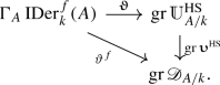
• (iv) Let us denote $\Gamma _A M$ the universal power divided algebra of the A-module M and $\gamma _m: M \rightarrow \Gamma _A M$, $m\ge 1$, the universal power divided maps (cf. [1, Appendix A]). There are unique maps of graded A-algebras

  $$\begin{aligned} \vartheta ^f: \Gamma _A {{\,\mathrm{IDer}\,}}^f_k(A) \rightarrow {{\,\mathrm{\text {gr}}\,}}{\mathcal {D}}_{A/k},\quad {\varvec{\upvartheta }}:\Gamma _A {{\,\mathrm{IDer}\,}}^f_k(A) \rightarrow {{\,\mathrm{\text {gr}}\,}}\mathbb {U}_{A/k}^{\text {HS}} \end{aligned}$$

  such that $\vartheta ^f {\scriptstyle \,\circ \,}\gamma _m = \chi ^m$ and ${\varvec{\upvartheta }}{\scriptstyle \,\circ \,}\gamma _m = {\varvec{\upchi }}^m$ for all $m\ge 1$ (see (2.6) in [10]⁴ and Corollary 3.4.3 of [13]). Moreover, the following diagram is commutative:

  

• (v) If ${{\,\mathrm{IDer}\,}}^f_k(A)={{\,\mathrm{Der}\,}}_k(A)$, then the map ${\varvec{\upvartheta }}:\Gamma _A {{\,\mathrm{IDer}\,}}^f_k(A) \longrightarrow {{\,\mathrm{\text {gr}}\,}}\mathbb {U}_{A/k}^{\text {HS}}$ is surjective (see Proposition 3.4.4 of [13]).

After Proposition 2.1.7, the HS-structure $\Upsilon$ on $\mathbb {U}_{A/k}^{\text {HS}}$ over A / k (see Proposition 2.2.1) induces a natural LR-admissible map $\nabla ^{\text {HS}}: {{\,\mathrm{Der}\,}}_k(A) \rightarrow \mathbb {U}_{A/k}^{\text {HS}}$ given by

$$\begin{aligned} \Upsilon ^1_1(\text {Id}+\delta s) = 1 + \nabla ^{\text {HS}}(\delta ) s,\quad \forall \delta \in {{\,\mathrm{Der}\,}}_k(A), \end{aligned}$$

which in turn induces a unique map of k-algebras over A:

$$\begin{aligned} {\varvec{\kappa }}: \mathbb {U}_{A/k}^{\text {LR}} \rightarrow \mathbb {U}_{A/k}^{\text {HS}} \end{aligned}$$

(12)

such that ${\varvec{\kappa }}{\scriptstyle \,\circ \,}\sigma = \nabla ^{\text {HS}}$, which is obviously filtered and ${\varvec{\upupsilon }}^{\text {HS}} {\scriptstyle \,\circ \,}{\varvec{\kappa }}= {\varvec{\upupsilon }}^{\text {LR}}$.

The goal of this section is to prove the main result of this paper, namely, if ${\mathbb {Q}}\subset k$, then the map (12) is an isomorphism.

From now on, we assume that ${\mathbb {Q}}\subset k$. Let R be a k-algebra over A endowed with a LR-admissible map $\nabla : {{\,\mathrm{Der}\,}}_k(A) \rightarrow R$ (see Definition 2.1.4).

Theorem 2.2.5

Under the above hypotheses, there is a unique HS-structure $\Psi = \left\{ \Psi ^p_\Delta \right\}$ on R over A / k such that for each $p\ge 1$ and each non-empty co-ideal $\Delta \subset {\mathbb {N}}^p$, the following diagram is commutative:

where we denote $\mathbf s =\{s_1,\dots ,s_p\}$ and ${\overline{\nabla }}:{{\,\mathrm{Der}\,}}_k(A)[[\mathbf s ]]_{\Delta ,+} \rightarrow R[[\mathbf s ]]_{\Delta ,+}$ the left $A[[\mathbf s ]]_\Delta$-linear map induced by $\nabla$:

$$\begin{aligned} {\overline{\nabla }} \left( \sum \delta _\alpha \mathbf s ^\alpha \right) = \sum \nabla (\delta _\alpha ) \mathbf s ^\alpha . \end{aligned}$$

Moreover, if $R = \cup _{d\ge 0} R_d$ is filtered and ${{\,\mathrm{Im}\,}}\nabla \subset R_1$, then $\Psi$ is a filtered HS-structure.

Proof

We define $\Psi ^p_\Delta :{{\,\mathrm{HS}\,}}^p_k(A;\Delta ) \longrightarrow {{\,\mathrm{{\mathcal {U}}}\,}}^p(R;\Delta )$ by forcing the diagram in the statement to be commutative. Remember that the vertical arrows $\varepsilon$ are bijective from Proposition 1.2.11 and (9). To simplify, let us write $\Psi = \Psi ^p_\Delta$. For each $E\in {{\,\mathrm{HS}\,}}^p_k(A;\Delta )$ we have $\varepsilon (\Psi (E)) = {\overline{\nabla }}(\varepsilon (E))$, i.e.:

$$\begin{aligned} {\varvec{\chi }}(\Psi (E)) = \Psi (E) \, {\overline{\nabla }}(\varepsilon (E)) \Longleftrightarrow |\alpha | \Psi (E)_\alpha = \sum _{\begin{array}{c} \scriptscriptstyle \beta +\gamma = \alpha \\ \scriptscriptstyle |\beta |>0 \end{array}} \Psi (E)_\gamma \, \nabla (\varepsilon _\beta (E))\ \forall \alpha \in \Delta . \end{aligned}$$

Actually, we have a bigger commutative diagram:

[see (9)] with $\overline{{\overline{\nabla }}} \left( \{\delta ^i\}_{i=1}^p \right) = \{{\overline{\nabla }}(\delta ^i)\}_{i=1}^p$ and $\varepsilon = \Sigma {\scriptstyle \,\circ \,}{\varvec{\varepsilon }}$. In particular, for each $E\in {{\,\mathrm{HS}\,}}^p_k(A;\Delta )$ and each $i=1,\dots ,p$ we have ${\varvec{\chi }}^i(\Psi (E)) = \Psi (E) \, {\overline{\nabla }}(\varepsilon ^i (E))$ and ${\varvec{\chi }}(\Psi (E)) = \Psi (E) \, {\overline{\nabla }}(\varepsilon (E))$, or equivalently:

$$\begin{aligned} \alpha _i \Psi (E)_\alpha = \sum _{\begin{array}{c} \scriptscriptstyle \beta +\gamma = \alpha \\ \scriptscriptstyle |\beta _i|>0 \end{array}} \Psi (E)_\gamma \, \nabla (\varepsilon ^i_\beta (E))\ \text { and }\ |\alpha | \Psi (E)_\alpha = \sum _{\begin{array}{c} \scriptscriptstyle \beta +\gamma = \alpha \\ \scriptscriptstyle |\beta |>0 \end{array}} \Psi (E)_\gamma \, \nabla (\varepsilon _\beta (E)), \end{aligned}$$

for all $\alpha \in \Delta$.

First, we will prove that the $\Psi$ are group homomorphisms. Let us take $D,E\in {{\,\mathrm{HS}\,}}^p_k(A;\Delta )$. In order to prove $\Psi (D{\scriptstyle \,\circ \,}E) = \Psi (D)\, \Psi (E)$ it is enough to prove that:

$$\begin{aligned} {\overline{\nabla }} (\varepsilon (D{\scriptstyle \,\circ \,}E)) = \varepsilon \left( \Psi (D{\scriptstyle \,\circ \,}E) \right) = \varepsilon \left( \Psi (D)\, \Psi (E) \right) , \end{aligned}$$

(13)

but we know that [see 1.2.9, (i)]:

$$\begin{aligned}&\varepsilon (D{\scriptstyle \,\circ \,}E) = E^*\, \varepsilon (D)\, E + \varepsilon (E), \\&\quad \varepsilon \left( \Psi (D)\, \Psi (E) \right) = \Psi (E)^* \, \varepsilon \left( \Psi (D)\right) \, \Psi (E) + \varepsilon \left( \Psi (E)\right) \\&\quad = \Psi (E)^* \, {\overline{\nabla }} (\varepsilon (D))\, \Psi (E) + {\overline{\nabla }} (\varepsilon (E)), \end{aligned}$$

and so identity (13) is equivalent to:

$$\begin{aligned} {\overline{\nabla }} (E^*\, \varepsilon (D) \, E)) = \Psi (E)^* \, {\overline{\nabla }} (\varepsilon ( D)) \, \Psi (E), \end{aligned}$$

(14)

which is a consequence of Lemma 2.2.6.⁵

Second, let us prove that $\Psi (D)$ is a D-element for each $D\in {{\,\mathrm{HS}\,}}_k^p(A;\Delta )$, i.e.:

$$\begin{aligned} \Psi (D)_\alpha \, a = \sum _{\scriptscriptstyle \beta +\gamma =\alpha } D_\beta (a)\, \Psi (D)_\gamma \quad \forall \alpha \in \Delta ,\ \forall a\in A. \end{aligned}$$

For $\alpha =0$ the equality being clear, we proceed by induction on $|\alpha |$:

$$\begin{aligned}&\displaystyle |\alpha | \Psi (D)_\alpha \, a = \sum _{\begin{array}{c} \scriptscriptstyle \beta +\gamma = \alpha \\ \scriptscriptstyle |\beta |>0 \end{array}} \Psi (D)_\gamma \, \nabla (\varepsilon _\beta (D)) \, a \\&\quad {\mathop {=}\limits ^{(\star )}} \quad \displaystyle \sum _{\begin{array}{c} \scriptscriptstyle \beta +\gamma = \alpha \\ \scriptscriptstyle |\beta |>0 \end{array}} \Psi (D)_\gamma \, a \, \nabla (\varepsilon _\beta (D)) + \sum _{\begin{array}{c} \scriptscriptstyle \beta +\gamma = \alpha \\ \scriptscriptstyle |\beta |>0 \end{array}} \Psi (D)_\gamma \, \varepsilon _\beta (D)(a) \\&\quad {\mathop {=}\limits ^{\text {(IH)}}} \displaystyle \sum _{\begin{array}{c} \scriptscriptstyle \beta +\gamma '+\gamma ''= \alpha \\ \scriptscriptstyle |\beta |>0 \end{array}} D_{\gamma '}(a)\, \Psi (D)_{\gamma ''} \, \nabla (\varepsilon _\beta (D)) + \sum _{\begin{array}{c} \scriptscriptstyle \beta +\gamma '+\gamma ''= \alpha \\ \scriptscriptstyle |\beta |>0 \end{array}} D_{\gamma '}(\varepsilon _\beta (D)(a))\, \Psi (D)_{\gamma ''} \\&\quad = \displaystyle \sum _{\begin{array}{c} \scriptscriptstyle \gamma '+\mu = \alpha \\ \scriptscriptstyle |\mu |>0 \end{array}} D_{\gamma '}(a)\, \left( \sum _{\begin{array}{c} \scriptscriptstyle \beta +\gamma ''= \mu \\ \scriptscriptstyle |\beta |>0 \end{array}} \Psi (D)_{\gamma ''} \, \nabla (\varepsilon _\beta (D)) \right) \\&\qquad + \displaystyle \sum _{\begin{array}{c} \scriptscriptstyle \nu +\gamma ''= \alpha \\ \scriptscriptstyle |\nu |>0 \end{array}} \left( \sum _{\begin{array}{c} \scriptscriptstyle \beta +\gamma '= \nu \\ \scriptscriptstyle |\beta |>0 \end{array}} (D_{\gamma '} {\scriptstyle \,\circ \,}\varepsilon _\beta (D))(a) \right) \, \Psi (D)_{\gamma ''}= \sum _{\begin{array}{c} \scriptscriptstyle \gamma '+\mu = \alpha \\ \scriptscriptstyle |\mu |>0 \end{array}} |\mu | \, D_{\gamma '}(a)\, \Psi (D)_\mu \\&\qquad + \displaystyle \sum _{\begin{array}{c} \scriptscriptstyle \nu +\gamma ''= \alpha \\ \scriptscriptstyle |\nu |>0 \end{array}} |\nu |\, D_\nu (a) \, \Psi (D)_{\gamma ''}= |\alpha | \sum _{\scriptscriptstyle \beta +\gamma =\alpha } D_\beta (a)\, \Psi ^p_\Delta (D)_\gamma . \end{aligned}$$

Notice that that equality $(\star )$ uses that $\nabla$ satisfies Leibniz rule.

To finish, it remains to prove that for any substitution map $\varphi : A[[\mathbf s ]]_\Delta \rightarrow A[[\mathbf t ]]_\Omega$, with $\mathbf t =\{t_1,\dots ,t_q\}$ and $\Omega \subset {\mathbb {N}}^q$ a non-empty co-ideal, and any $D\in {{\,\mathrm{HS}\,}}^p_k(A;\Delta )$ we have:

$$\begin{aligned} \Psi ^q_\Omega (\varphi {\scriptstyle \bullet }D) = \varphi {\scriptstyle \bullet }\Psi ^p_\Delta (D). \end{aligned}$$

This is equivalent to ${\varvec{\varepsilon }}(\Psi ^q_\Omega (\varphi {\scriptstyle \bullet }D)) = {\varvec{\varepsilon }}(\varphi {\scriptstyle \bullet }\Psi ^p_\Delta (D))$, but we know from Theorem 1.5.2 that:

$$\begin{aligned}&\displaystyle \varepsilon ^j_e(\varphi {\scriptstyle \bullet }\Psi ^p_\Delta (D)) = \sum _{\begin{array}{c} \scriptscriptstyle 0<|h|\le |e|\\ \scriptscriptstyle i\in {{\,\mathrm{\text {supp}}\,}}h \end{array}} \mathbf N ^{j,i}_{e,h} \varepsilon ^i_h(\Psi ^p_\Delta (D)) = \sum _{\begin{array}{c} \scriptscriptstyle 0<|h|\le |e|\\ \scriptscriptstyle i\in {{\,\mathrm{\text {supp}}\,}}h \end{array}} \mathbf N ^{j,i}_{e,h} \nabla (\varepsilon ^i_h(D)) \\&\quad \displaystyle {\mathop {=}\limits ^{(\star \star )}} \nabla \left( \sum _{\begin{array}{c} \scriptscriptstyle 0<|h|\le |e|\\ \scriptscriptstyle i\in {{\,\mathrm{\text {supp}}\,}}h \end{array}} \mathbf N ^{j,i}_{e,h} \varepsilon ^i_h(D) \right) = \nabla ( \varepsilon ^j_e(\varphi {\scriptstyle \bullet }D) ) = \varepsilon ^j_e( \Psi ^q_\Omega (\varphi {\scriptstyle \bullet }D) ) \end{aligned}$$

for all $j=1,\dots ,q$ and for all $e\in \Omega$, and we are done. Let us notice that equality $(\star \star )$ uses that $\nabla$ is A-linear.

For the last part, if $R = \cup _{d\ge 0} R_d$ is filtered and ${{\,\mathrm{Im}\,}}\nabla \subset R_1$, then the image of each map

$$\begin{aligned} {\overline{\nabla }}: {{\,\mathrm{Der}\,}}_k(A)[[\mathbf s ]]_{\Delta ,+} \longrightarrow R[[\mathbf s ]]_{\Delta ,+} \end{aligned}$$

is contained in $R_1[[\mathbf s ]]_{\Delta ,+}$, and it is easy to see that $\varepsilon ^{-1} \left( R_1[[\mathbf s ]]_{\Delta ,+} \right) \subset {{\,\mathrm{{\mathcal {U}}}\,}}_{\text {fil}}^p(R;\Delta )$. $\square$

Lemma 2.2.6

Under the hypotheses of Theorem 2.2.5, for each $\delta \in {{\,\mathrm{Der}\,}}_k(A)[[\mathbf s ]]_\Delta$ and each $E\in {{\,\mathrm{HS}\,}}^p_k(A;\Delta )$ the following identity holds:

$$\begin{aligned} \Psi (E) \, {\overline{\nabla }} (E^*\, \delta \, E) = {\overline{\nabla }} (\delta ) \, \Psi (E). \end{aligned}$$

Proof

Since all the involved maps and operations are compatible with truncations and any series in $R[[\mathbf s ]]_\Delta$ is determined by its finite truncations, we may assume that $\Delta$ is finite, and since both terms are $k[[\mathbf s ]]_\Delta$-linear in $\delta$, we may assume $\delta \in {{\,\mathrm{Der}\,}}_k(A)$. By definition of $\Psi$, we have:

$$\begin{aligned} {\varvec{\chi }}(\Psi (E)) = \Psi (E) \, {\overline{\nabla }}(\varepsilon (E)),\quad \text {with}\ {\varvec{\chi }}= \sum _{i=1}^p s_i \frac{\partial }{\partial s_i}. \end{aligned}$$

Since the 0-term of the series $\Psi (E) \, {\overline{\nabla }} (E^*\, \delta \, E)$ and ${\overline{\nabla }} (\delta ) \, \Psi (E)$ coincide (they are equal to $\nabla (\delta )$) and ${\mathbb {Q}}\subset k$, it is enough to prove that both series are solution of the differential equation:

$$\begin{aligned} {\varvec{\chi }}(Y) = Y \, {\overline{\nabla }}(\varepsilon (E)). \end{aligned}$$

Namely:

$$\begin{aligned}&\displaystyle {\varvec{\chi }}\left( \Psi (E) \, {\overline{\nabla }} (E^*\, \delta \, E) \right) = {\varvec{\chi }}(\Psi (E)) \, {\overline{\nabla }} (E^*\, \delta \, E) + \Psi (E) \, {\varvec{\chi }}({\overline{\nabla }} (E^*\, \delta \, E) ) \\&\quad =\displaystyle \Psi (E)) \, {\overline{\nabla }}(\varepsilon (E)) \, {\overline{\nabla }} (E^*\, \delta \, E) + \Psi (E) \, {\overline{\nabla }} ({\varvec{\chi }}(E^*\, \delta \, E) ) \\&\quad = \displaystyle \Psi (E)) \, {\overline{\nabla }}(\varepsilon (E)) \, {\overline{\nabla }} (E^*\, \delta \, E) + \Psi (E) \, {\overline{\nabla }} ({\varvec{\chi }}(E^*) \, \delta \, E + E^*\, \delta \, {\varvec{\chi }}(E)) \\&\quad {\mathop {=}\limits ^{(\star )}} \displaystyle \Psi (E)) \, {\overline{\nabla }}(\varepsilon (E)) \, {\overline{\nabla }} (E^*\, \delta \, E) + \Psi (E) \, {\overline{\nabla }} ( - \varepsilon (E) \, E^* \, \delta \, E + E^*\, \delta \, E \, \varepsilon (E)) \\&\quad =\displaystyle \Psi (E)) \, {\overline{\nabla }}(\varepsilon (E)) \, {\overline{\nabla }} (E^*\, \delta \, E) + \Psi (E) \, {\overline{\nabla }} ( [E^*\, \delta \, E,\varepsilon (E)]) \\&\quad = \displaystyle \Psi (E)) \, {\overline{\nabla }} (\varepsilon (E)) \, {\overline{\nabla }} (E^*\, \delta \, E) + \Psi (E) \, [{\overline{\nabla }}(E^*\, \delta \, E),{\overline{\nabla }}(\varepsilon (E))] \\&\quad = \displaystyle \Psi (E)) \, {\overline{\nabla }} (E^*\, \delta \, E) \, {\overline{\nabla }}(\varepsilon (E)), \end{aligned}$$

where equality $(\star )$ comes from 1.2.9, (ii), and

$$\begin{aligned} {\varvec{\chi }}({\overline{\nabla }}(\delta )\, \Psi (E)) = {\overline{\nabla }}(\delta )\, {\varvec{\chi }}(\Psi (E)) = {\overline{\nabla }}(\delta )\, \Psi (E)\, {\overline{\nabla }}(\varepsilon (E)). \end{aligned}$$

$\square$

Theorem 2.2.7

If ${\mathbb {Q}}\subset k$, then the map (12)

$$\begin{aligned} {\varvec{\kappa }}: \mathbb {U}_{A/k}^{\text {LR}} \rightarrow \mathbb {U}_{A/k}^{\text {HS}} \end{aligned}$$

is an isomorphism of filtered k-algebras over A.

Proof

By applying Theorem 2.2.5 to the universal LR-admissible map

$$\begin{aligned} \sigma :{{\,\mathrm{Der}\,}}_k(A) \longrightarrow \mathbb {U}_{A/k}^{\text {LR}}, \end{aligned}$$

there is a unique filtered HS-structure $\Psi ^{\text {LR}}$ on $\mathbb {U}_{A/k}^{\text {LR}}$ over A / k such that ${\overline{\sigma }} {\scriptstyle \,\circ \,}\varepsilon =\varepsilon {\scriptstyle \,\circ \,}\left( \Psi ^{\text {LR}}\right) ^p_\Delta$ for each $p\ge 1$ and each non-empty co-ideal $\Delta \subset {\mathbb {N}}^p$, and so, by Proposition 2.2.1, there is a unique map ${\varvec{\lambda }}: \mathbb {U}_{A/k}^{\text {HS}} \longrightarrow \mathbb {U}_{A/k}^{\text {LR}}$ of filtered k-algebras over A such that $\Psi ^{\text {LR}} = {\varvec{\lambda }}{\scriptstyle \,\circ \,}\Upsilon$.

Let us prove that ${\varvec{\lambda }}$ is the inverse map of ${\varvec{\kappa }}$. For each $\delta \in {{\,\mathrm{Der}\,}}_k(A)$ we have:

$$\begin{aligned}&\sigma (\delta ) s = {\overline{\sigma }}(\delta s) = {\overline{\sigma }}(\varepsilon (\text {Id}+ \delta s)) = \varepsilon \left( \left( \Psi ^{\text {LR}}\right) ^1_1(\text {Id}+ \delta s)\right) = \varepsilon ({\overline{{\varvec{\lambda }}}}(\Upsilon ^1_1(\text {Id}+ \delta s))) = \\&\quad \varepsilon ({\overline{{\varvec{\lambda }}}}(1 + \nabla ^{\text {HS}}(\delta ) s)) = \varepsilon (1+ {\varvec{\lambda }}(\nabla ^{\text {HS}}(\delta ))s) = ({\varvec{\lambda }}{\scriptstyle \,\circ \,}\nabla ^{\text {HS}})(\delta )s. \end{aligned}$$

So, $\sigma = {\varvec{\lambda }}{\scriptstyle \,\circ \,}\nabla ^{\text {HS}} = {\varvec{\lambda }}{\scriptstyle \,\circ \,}{\varvec{\kappa }}{\scriptstyle \,\circ \,}\sigma$ and we deduce that ${\varvec{\lambda }}{\scriptstyle \,\circ \,}{\varvec{\kappa }}= \text {Id}$.

Since ${\mathbb {Q}}\subset k$, we have ${{\,\mathrm{IDer}\,}}^f_k(A)={{\,\mathrm{Der}\,}}_k(A)$ and so the map ${\varvec{\upvartheta }}:\Gamma _A {{\,\mathrm{IDer}\,}}^f_k(A) \rightarrow {{\,\mathrm{\text {gr}}\,}}\mathbb {U}_{A/k}^{\text {HS}}$ is surjective (see 2.2.4, (v)). We easily check that the following diagram is commutative:

and since ${\mathbb {Q}}\subset k$, we have ${{\,\mathrm{Sym}\,}}_A {{\,\mathrm{Der}\,}}_k(A) \xrightarrow {\sim } \Gamma _A {{\,\mathrm{Der}\,}}_k(A)$ and we deduce that ${{\,\mathrm{\text {gr}}\,}}{\varvec{\kappa }}$ is surjective, and so ${\varvec{\kappa }}$ is surjective too. We conclude that ${\varvec{\lambda }}$ is the the inverse map of ${\varvec{\kappa }}$. $\square$

Corollary 2.2.8

Under the above hypotheses, the category of left (resp. right) HS-modules over A / k coincide with the category of A-modules endowed with a left (resp. right) integrable connection over A / k.

References

Berthelot, P., Ogus, A.: Notes on Crystalline Cohomology. Mathematical Notes, vol. 21. Princeton University Press, Princeton (1978)
Brown, W.C.: On the embedding of derivations of finite rank into derivations of infinite rank. Osaka J. Math. 15, 381–389 (1978)
Deligne, P.: Equations Différentielles à Points Singuliers Réguliers. Lecture Notes in Mathematics, vol. 163. Springer, Berlin (1970)
Grothendieck, A.: Éléments de Géométrie Algébrique (Rédigés Avec la Collaboration de Jean Dieudonné): IV. Étude Locale des Schémas et de Morphismes de Schémas, Quatrième Partie. Publ. Math. Inst. Hautes Études Sci, vol. 32. Press University de France, Paris (1967)
Hasse, H., Schmidt, F.K.: Noch eine Begründung der theorie der höheren differrentialquotienten in einem algebraischen Funktionenkörper einer Unbestimmten. J. Reine Angew. Math. 177, 223–239 (1937)
Huebschmann, J.: Duality for Lie-Rinehart algebras and the modular class. J. Reine Angew. Math. 510, 103–159 (1999)
Matsumura, H.: Integrable derivations. Nagoya Math. J. 87, 227–245 (1982)
Matsumura, H.: Commutative Ring Theory. Cambridge Studies in Advanced Mathematics, vol. 8. Cambridge University Press, Cambridge (1986)
Mirzavaziri, M.: Characterization of higher derivations on algebras. Comm. Algebra 38(3), 981–987 (2010)
Narváez Macarro, L.: Hasse-Schmidt derivations, divided powers and differential smoothness. Ann. Inst. Fourier (Grenoble) 59(7), 2979–3014 (2009)
Narváez Macarro, L.: On the modules of \(m\)-integrable derivations in non zero characteristic. Adv. Math. 229(5), 2712–2740 (2012)
Narváez Macarro, L.: On Hasse–Schmidt derivations: the action of substitution maps. In: “Singularities, Algebraic Geometry, Commutative Algebra, and Related Topics. Festschrift for Antonio Campillo on the Occasion of his 65th Birthday”, 219–262. Springer International Publishing, Cham, 2018
Narváez Macarro, L.: Rings of differential operators as enveloping algebras of Hasse–Schmidt derivations. J. Pure Appl. Algebra 224(1), 320–361 (2020)
Narváez Macarro, L.: Hasse–Schmidt derivations versus classical derivations. In: “A panorama of Singularities”. Contemporary Mathematics, Amer. Math. Soc., Providence, RI, to appear. (arXiv:1810.08075)
Rinehart, G.S.: Differential forms on general commutative algebras. Trans. Am. Math. Soc. 108, 195–222 (1963)
Author information
Authors and Affiliations
Corresponding author
Ethics declarations
Funding
Funding was provided by Ministerio de Economía, Industria y Competitividad, Gobierno de España (Grant No. MTM2016-75027-P) and Consejería de Economía, Innovación, Ciencia y Empleo, Junta de Andalucía (Grant No. P12-FQM-2696).
Additional information
Publisher's Note
Springer Nature remains neutral with regard to jurisdictional claims in published maps and institutional affiliations.
Partially supported by MTM2016-75027-P, P12-FQM-2696 and FEDER.
Rights and permissions
About this article
Cite this article
Narváez Macarro, L. Hasse–Schmidt modules versus integrable connections. Rev Mat Complut 34, 75–98 (2021). https://doi.org/10.1007/s13163-019-00340-z
Received:
Accepted:
Published:
Issue Date:
DOI: https://doi.org/10.1007/s13163-019-00340-z
Keywords
- Hasse–Schmidt derivation
- Integrable derivation
- Differential operator
- Substitution map
- HS-structure
- Integrable connection