

- EAER>
- Journal Archive>
- Contents>
- articleView
Contents
Citation
| No | Title |
|---|
Article View
East Asian Economic Review Vol. 22, No. 1, 2018. pp. 75-114.
DOI https://dx.doi.org/10.11644/KIEP.EAER.2018.22.1.339
Number of citation : 0View
214
Download
125
Equivalence between Increasing Returns and Comparative Advantage as the Determinants of Intra-industry Trade: An Industry Analysis for Korea

Abstract
A two-part model is estimated to see if increasing returns and comparative advantage are empirically equivalent in explaining intra-industry trade. The model has separate mechanisms for determining the occurrence and the extent of intra-industry trade. Estimation is based on an augmented Grubel-Lloyd index derived from the data set on SITC 7 goods at the 3-digit SITC (Revision 4) for country pairs in which Korea is fixed as a source country. Estimation results show that both increasing returns and comparative advantage can explain the occurrence and the extent of intra-industry trade.
JEL Classification: F11, F12, F14
Keywords
Grubel-Lloyd Index, Increasing Returns, Comparative Advantage, Intra-industry Trade, Trade Costs, Export Margins, Two-part Model
I. INTRODUCTION
There are two stylized arguments about intra-industry trade in the literature. The first argument is that comparative advantage and increasing returns are equivalent in explaining the occurrence of intra-industry trade. That intra-industry trade can arise in comparative advantage as well as in increasing returns models (e.g. Harrigan, 1994) has been widely recognized ever since monopolistic competition with increasing returns was identified as the driver of intra-industry trade (e.g. Krugman, 1979; Helpman and Krugman, 1985).1 The second argument is that the two causes of trade have opposite influence on the expansion of intra-industry trade. The asymmetric influence argument emphasizes specific connections that are supposed to exist between intra-industry trade and its causes: the extent of intra-industry trade is negatively related to comparative advantage, but positively to increasing returns (e.g. Greenaway et al., 1995; Hummels and Levinsohn, 1995).
The arguments about the relationship between intra-industry trade and the two causes of trade are not always
This paper aims to investigate whether the two strands of arguments about intra-industry trade are compatible with Korea’s trade data. Specifically, it tries to examine if equivalence arises between the causes of trade in explaining the occurrence of Korea’s intra-industry trade, and if specific connections exist between the extent of Korea’s intra-industry trade and its causes. For that investigation, this paper adapts a two-part model for the Grubel-Lloyd (GL) index of intra-industry trade. The GL index is a corner solution response variable, which not only has a continuous distribution over strictly positive values, but also takes on a zero value with positive probability (Wooldridge, 2010: 667). What is advantageous about the GL index for investigating the relationship between intra-industry trade and its causes is that it can be expressed as a function of ‘normalized unit costs’ (representing comparative advantage) and ‘fixed trade costs’ (representing increasing returns).2 Such transformation facilitates estimation which uses a two-part model that allows different mechanisms for the choice of trade types (i.e. intra-industry versus interindustry trade) on the one hand and the expansion of intra-industry trade attributable to each cause of trade on the other (Wooldridge, 2010: 690-703). The idea of using a two-part model is justifiable since profit maximizing firms’ decisions on specialization may result in zero trade for some bilateral trading relations (i.e. “participation decision” or a zero GL index), but may lead to strictly positive trade for others once intra-industry trade occurs (i.e. “amount decision” or a positive GL index). The extent of intra-industry trade may be quite differently determined than the probability of its occurrence.
Estimation proceeds in two parts: the first part estimates the probability of intra-industry trade to occur, and the second part estimates the extent of intra-industry trade once it occurs. If there exists an empirical equivalence between increasing returns and comparative advantage, the estimated coefficients on these causes of trade will have the same sign, if not the same magnitude, in the occurrence equation (i.e. the first part of the model). On the other hand, if there are specific connections between intra-industry trade and its causes, they will be verified by the estimates of the competing causes of trade in the extent equation (i.e. in the second part of the model). The data used in this paper are trade flows in SITC 7 goods at the 3-digit SITC (Revision 4) compiled from the UN Commodity Trade Statistics Database for country pairs in which Korea is fixed as a source country. The SITC 7 data have been intentionally chosen because, as Bergstrand (1990: 1224) argued, the industry groups comprising SITC 7 are representative of most manufacturing industries.
Estimation results show that, in the extent equation (for a censored data set of the strictly positive intra-industry trade indexes), the GL index is positively related to both increasing returns and comparative advantage. The coefficients on the competing causes of trade in the GL index have the same positive signs. Both causes of trade expand the extent of intra-industry trade. Similarly, in the occurrence equation (for an uncensored data set of the nonnegative intra-industry trade indexes in which sample types are not discriminated), both increasing returns and comparative advantage have positive effects on the
Earlier investigations focused on the effects of country- and industry-specific determinants on the intensity of intra-industry trade (e.g. Loertscher and Wolter, 1980; Greenaway and Milner, 1984; Bergstrand, 1990; and Greenaway et al., 1995). In particular, Greenaway et al. (1995) separated total intra-industry trade into vertical and horizontal parts, and related them separately to industry specificities such as product differentiation, scale economies, and market structure.3 Dividing the total GL index into the horizontal and vertical indexes would have helped avoid ambiguity about the expected signs of some determinants because information priors could then be used more distinctively under discriminating specification.4 However, vertical and horizontal GL indexes in Greenaway et al. (1995) were arbitrarily assigned dependent variables with different data sets each represented by comparative advantage and increasing returns respectively.
In this paper, however, comparative advantage and increasing returns are not dependent but explanatory variables. Their causal relationship to the GL index testifies the equivalence between them in explaining within-industry trade and identifies the characteristic connections between intra-industry trade and its causes. Both causes of trade can explain the occurrence and the extent of intra-industry trade, although they are not alike in the magnitude of influence. The equivalence between the causes of trade in predicting the occurrence of intra-industry trade is already corroborated in theoretical investigations. For example, Weder (1995) showed that comparative advantage based on differences in demand across countries could cause intra-industry trade.5 Davis and Weinstein (1996) also showed that idiosyncratic demand is crucial in determining trade patterns not only in comparative advantage but also in increasing returns models. This happens because the relative (not absolute) market size matters for production patterns, while the relative demand plays a crucial role in assigning production of goods across countries.
The results in this paper, however, are not consistent with the predictions of the Helpman-Krugman model, in which interindustry trade is motivated by comparative advantage, while intra-industry trade is motivated by increasing returns. The estimation results in this paper do not support a unified account of intra-industry and interindustry trade that associates intra-industry trade with relative country size (i.e. increasing returns), and interindustry trade with relative factor abundance (i.e. comparative advantage). On the other hand, the results in this paper are much stronger than the findings in Hummels and Levinsohn (1995), in which differences in factor endowment are not as effective in explaining intra-industry and interindustry trade as country specific differences in geography, cultural and language ties, trade barriers, or endowments of land.6
This paper also contrasts with Evenett and Keller (2002), in which neither increasing returns nor comparative advantage could single-handedly replicate the predictions of the gravity model. Instead, Evenett and Keller showed that the hybrid model of increasing returns and comparative advantage better supported the predictions of the gravity equation for the samples with high GL index values, while the ‘unicone’ factor-proportions model (i.e. a diversified comparative advantage model) did it for the samples with low GL index values. Deriving the support for imperfect specialization models, Evenett and Keller in effect established that the two causes of trade should differ from each other in explaining the extent of intra-industry trade.
The rest of the paper is organized as follows. Section II introduces empirical methods. Section III reports empirical results, and Section IV concludes.
1)Intra-industry trade arises in a monopolistic competition model if international exploitation of scale economies induces concentrated production of a variety commonly demanded across countries
2)The conventional GL index by construction does not differentiate increasing returns and comparative advantage. The GL index just focuses on the degree of concurrence in exporting and importing between a pair of countries. The larger GL index merely indicates the more equal amount of goods exported and imported simultaneously, while the smaller GL index an increase in the amount of goods either imported or exported but not both.
3)
4)
5)When countries differ in the demand for differentiated products within an industry, home market advantage leads to intra-industry trade
6)In
II. EMPIRICAL STRATEGY
1. The Grubel-Lloyd Index
The Grubel-Lloyd index between countries  (country
  (country

The export and import components of the GL index are defined as in Chaney (2008). (See the Appendix A for details.)

where  and ‘fixed trade costs’
  so that it will increase if unit costs and/or fixed trade costs fall.
Dividing exports by imports in equation (1) transforms the GL index into a function of the export-import ratio 

The export-import ratio  in turn is a function of ‘normalized unit costs’ and ‘fixed trade costs’ if consumer preferences are identical across countries (i.e. for the common budget share
  (See equations (A-10A) and (A-10B) in the Appendix A.) With simple substitution,
  becomes a function of increasing returns (through fixed trade costs
  and comparative advantage (through normalized unit costs
The connections between intra-industry trade and the competing causes of trade in the GL index are identified because of the variable and fixed costs that profit maximizing firms have to incur in the export market. Information about ‘fixed trade costs’ helps separate increasing returns and comparative advantage since their effects on trade flows differ depending not only on demand substitutability but also on firm heterogeneity.9 Similarly, information about ‘normalized unit costs’ (including transport costs) also helps discriminate comparative advantage and increasing returns because the ‘home market effect’ causes the two competing forces to yield the opposite predictions regarding the patterns of production and trade (Davis and Weinstein, 1996).10
The GL index above has some noticeable features. First, it allows of ‘imperfect specialization’ that nests increasing returns with comparative advantage as shown in Evenett and Keller (2002) and Davis and Weinstein (1996).11 Second, the GL index helps infer the effects of ‘fixed trade costs’ (or market entry costs) on bilateral trade flows as illustrated in Chaney (2008) that modified Melitz (2003) to show how market entry costs affect trade flows through the extensive and intensive margins of exports.12 The different levels of market entry costs distinguish firms from one another. Since only efficient firms can bear the burden of market entry costs with future export profits (but less efficient ones cannot), ‘fixed trade costs’ will set the limits to the extensive margin of exports. Third, the GL index helps deal with the effects of variable trade barriers on trade flows. Trade barriers separate countries in a way analogous to the Armington assumption, inducing changes in the intensive and extensive margins of exports.13
2. A Two-part Model
A two-part model (i.e. a lognormal hurdle model) is useful to estimating the relationship of the GL index with the causes of trade.14 The first part of the model consists of a binary equation  where
where  The second part of the model is a linear equation
  whose lognormal form is written as
  for which
  Combining both parts of the model yields the expectation as
 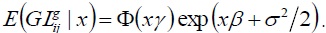 The discrete choice model uses all observations, while the conditional density model
 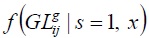 uses observations with
  only. The two parts of the model are usually assumed to be independent, and may have different regressors.
3. Regression Specification
For estimation, the GL index is specified in regression equation form as

where

where 
In dealing with ln  For that purpose, it is necessary to substitute the linear projection of
  from the regression of ln
  can be used instead. Still the OLS estimators of the following equation with will be consistent.

where is the fitted value of
4. Instrumentation
The setup above is conditioned on the availability of observations on ‘normalized unit costs’ and ‘fixed trade costs’  Yet information on ‘fixed trade (entry) costs’ is not readily available. To control for the data unavailability, observable export margins will be used in the following.17 The rationale is that export margins are inversely related to changes in ‘normalized unit costs’ and ‘fixed trade costs.’ For example, new firms enter the export market to profit from a reduction in ‘fixed trade costs,’ while incumbent firms expand exports in response to a reduction in ‘normalized unit costs’ (Hummels and Klenow, 2005: 706).
Further, the elasticities of export margins with respect to these unobserved costs are derived in Chaney (2008: 1715-1717), which would help infer ‘fixed trade costs’ (Hummels and Klenow, 2005; Chaney, 2008 and Helpman et al., 2008). The Appendix B describes how ‘normalized unit costs’ and ‘fixed trade costs’ are related to export margins through the Chaney elasticities. What is sufficient here, however, is to note in Table 1 that changes in ‘fixed trade costs,’  are negatively correlated with the extensive margin,
  Specifically, since changes in ‘fixed trade costs’ affect the extensive margin negatively, the extensive margin,
  can be used as an IV for ‘fixed trade costs,’
With the extensive margin in place of ‘fixed trade costs,’ equation (4) is rewritten as

where 
With simple substitution, equation (5) is expressed as

where  is the fitted value of
7)The GL index is a sum of the absolute differences between bilateral exports and imports divided by the total amount of bilateral trade. The calculations of the GL index start with classifying observations on bilateral trade flows between countries into two different categories, intra-industry and interindustry. The GL index varies from zero (i.e. if a country either exports or imports each of its products unilaterally, no intra-industry trade occurs) to one (i.e. if a country exports and imports the same number of varieties simultaneously, there is only intra-industry trade).
8)Aggregating  over entire industries yields the GL index between countries
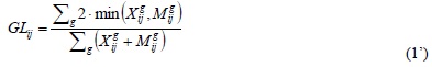
9)
10)In the presence of transport costs, the interaction between demand conditions and production opportunities (i.e. the home market effect) generates fundamentally different trade patterns for increasing returns and comparative advantage models
11)
12)
13)The
14)The two-part model is based on
15)Equation (3) is a first-degree Taylor series approximation of the log of the Grubel-Lloyd index (i.e. 
16)The control function approach is adopted from
17)Export margins explain how aggregate exports  increase through adjustments in the extensive (i.e. a change in the productivity threshold
  and intensive (i.e. a change in the volume of exports of an incumbent firm
  margins.
III. EMPIRICAL ANALYSIS
1. Data
The sample consists of data on SITC 7 goods at the 3-digit SITC (Revision 4) for country pairs, in which Korea is fixed as the reporter country during the period from 2007 to 2013. The bilateral trade flows data are from the UN Commodity Trade Statistics Database. The SITC 7 industry groups are selected because they are deemed to represent most manufacturing industries (Bergstrand, 1990: 1224).
The data on consumer price indexes (for multilateral resistance terms), output per worker in constant 2005 US dollars (for labor productivity adjusted unit costs), and trade costs are from the World Development Indicators, the ILO Database of Labor Statistics, and the ESCAP-World Bank International Trade Costs Database respectively. The other variables such as GDP and preferential trade agreements (FTAs) are from the World Bank and the World Trade Organization.
1) Dependent Variables
The dependent variable in equation (6),  is the ratio of Korea’s bilateral exports to imports with its trading partners at the 3-digit industry groups in SITC 7. The dependent variable in equation (7),
  is an average of bilateral Grubel-Lloyd indexes calculated over SITC 7 goods at the 3-digit SITC for country pairs in which Korea is the source country.
The number of exportable and importable items is thirty at the 3-digit SITC.18 The number of Korea’s bilateral trading partners in the data set is 197 for 3-digit industry groups in SITC 7. Forty one partners for which data other than trade flows were missing were excluded, which left usable data on bilateral trade flows for 156 countries. The total number of possible observations for the period from 2007 to 2013 between Korea and its trading partners is 1,092, of which 232 are zero trade flows. The number of trade in one direction only is 69, leaving the number of trade in both directions remaining at 791.While estimation proceeds on the same sample of data, the model uses a different data set for each part.19 Of all 1,092 bilateral trade relations, 791 data points are associated with intra-industry trade (i.e.  is positive), and only 69 observations with interindustry trade (i.e. is zero). The discrete choice model (i.e. the occurrence equation) of the two-part model uses all observations available on both intra-industry trade and zero-trade (i.e. 1023 data points). The conditional density model (i.e. the extent equation) where the response variable is positive uses observations on intra-industry trade only (i.e. 791 data points), which leaves observations on interindustry trade in effect censored.
2) Independent Variables
To substitute for comparative advantage (‘normalized unit costs’), the product of unit costs (labor productivity adjusted) and trade costs is divided by multilateral resistance terms. For labor productivity adjusted unit costs, output per worker data in constant 2005 US dollars is used whose data come from the ILO Database of Labor Statistics. Trade costs data are from the ESCAP-World Bank International Trade Costs Database. For multilateral resistance terms, consumer prices indexes are compiled from the World Development Indicators.
To get the measure of increasing returns (‘fixed trade costs’), the export margins of Korea for each destination country are calculated using the formulas given in Hummels and Klenow (2005: 710). For country

where

Korea’s average extensive margins calculated for 156 destination countries over the 2007-2013 period range from 0.356 (Bahamas) to 1.000 (China and Japan during 2007-2013, Indonesia during 2010-2013), while its average intensive margins range from 0.002 (Mauritania during 2011-2013) to 0.215 (Syria during 2008-2010). The means of the destination extensive and intensive margins over the period are 0.887 and 0.038 respectively.
The export margins show consistent patterns with regard to the competing causes of trade. The measure of comparative advantage (‘normalized unit costs’) is positively related to the intensive margin, while the extensive margin and the measure of comparative advantage are positively related to the GL index. These relationships are illustrated in Figure 1 to Figure 3.
In the two-part model, the occurrence equation may have an exogenous variable that is excluded from the extent equation. The excluded exogenous variable may change the probability of a positive outcome. Yet it should not affect the size of the extent of intra-industry trade once intra-industry trade occurs. Although it is difficult to find such a variable, having one in the occurrence equation will increase the precision of the estimates (Cameron and Trivedi, 2010: 561-562). For that reason, additional controls are included in the estimation equations. For example, common membership to FTAs or the log ratio of per capita GDP partner to per capita GDP Korea,  is controlled for. Common membership may facilitate the relocation of factor services, which may help increase intra-industry trade. Dummies for FTA membership assume one when trade occurs between Korea and its FTA partners. Relative income may also affect the demand for differentiated goods and intra-industry trade. The relative income data show consistent patterns with respect to intra-industry trade. The scatter plots show a positive relationship between
  in Figure 4. Controls for the destination country fixed effects are included in the fixed-effects equations to reflect special bilateral trade relationship. (For summary statistics, see Table C-1 in the Appendix C.)
2. Estimation Results
For reference, the export-import ratio and the GL index have been estimated using a single-equation method, in which three panel-data estimation methods have been used to allow for various assumptions about possible correlation between the unobserved effect in the error term and the explanatory variables. Estimates of single equations based on panel GLS (GLS), fixed-effects (FE), and random-effects (RE) methods are given in Table 2.
In the regression of the export-import ratio in Table 2, the coefficient on relative ‘normalized unit costs’ is negative and statistically significant except the fixed-effects model. What this implies is that comparative advantage does not necessarily expand unidirectional trade. Even though Korea’s trading partner is more productive (i.e. Korea’s trading partner has comparative advantage in terms of ‘normalized unit costs’), the gap between Korea’s exports and imports (i.e. its ‘trade balance’) may not widen because trade less tends to be carried out through inter-industry specialization (i.e. unidirectional trade) than through intra-industry specialization (i.e. bidirectional trade).
This result does not contradict the result obtained in the regression of the GL index, where the coefficient on relative ‘normalized unit costs’ is positive and significant except the fixed-effects model. In the regression of the GL index, a larger difference in ‘normalized unit costs’ between Korea and its trading partner makes trade more likely to be based on intra-industry specialization. Given common preferences across countries, intra-industry trade is inevitable if domestic production cannot replace foreign production because of technological disadvantage.
When it comes to the coefficient on relative ‘fixed trade costs,’ the export-import ratio is negatively related to smaller ‘fixed trade costs’ (i.e. a larger extensive margin), while the GL index is positively related. This indicates that the effects of increasing returns (‘fixed trade costs’) on the GL index and the export-import ratio are moving in the opposite direction. This makes sense because GL index measures the extent of intra-industry trade, while (the absolute value of the log of) the exportimport ratio the extent of interindustry trade.
The residual term  in the GL index that controls for the endogeneity of the export-import ratio
Regression on the pooled data shows that there is agreement in the signs of regression coefficients on the variables representing increasing returns and comparative advantage in explaining the extent of intra-industry trade. This implies that comparative advantage and increasing returns does not have discriminate influence on the extent of intra-industry trade measured by the GL index.
The coefficient estimates of the two-part model are presented in Table 3. Coefficients on ‘normalized unit costs’ and ‘fixed trade costs’ have positive signs both in the uncensored probit estimation (in which the intra-industry trade index is nonnegative) and in the censored linear estimation (in which the intra-industry trade index is strictly positive). An increase in ‘normalized unit costs’ and a decrease in ‘fixed trade costs’ (i.e. an increase in the extensive margin) would increase the probability of intra-industry trade to occur in a probit regression of  Again, in the extent of intra-industry trade regression, ‘normalized unit costs’ and ‘fixed trade costs’ have the same signs. Larger ‘normalized unit costs’ and smaller ‘fixed trade costs’ (i.e. a larger extensive margin) would increase the extent of intraindustry trade in a linear regression of
  on explanatory variables
Why is it that relative ‘normalized unit costs’ have a positive effect on the occurrence and the extent of intra-industry trade? First, the probability of intraindustry trade increases with relative ‘normalized unit costs’ because the likelihood of intra-industry specialization increases due to the widening productivity gap. Second, the effect of comparative advantage on the extent of intra-industry trade is positive. This could happen only if the decrease in the extent of intra-industry trade due to a reduction in the extensive margin (because fewer firms enter the export market due to a rise in the productivity threshold – with fewer varieties, there will be less room for intra-industry trade) is more than cancelled out by the increase in the extent of intra-industry due to a reduction in trade based on comparative advantage (a reduction in the intensive margin). If inter-industry trade based on comparative advantage decreases (i.e. a reduction in the intensive margin due to an increase in ‘normalized unit costs’), the room for intra-industry trade based on comparative advantage will increase since the possibility of intra-industry specialization will replace inter-industry trade.
The residual term  that controls for the endogeneity of the export-import ratio
The coefficient on ln(
The estimation results in Table 3 implicate that the variables representing comparative advantage and increasing returns are moving in the same direction in explaining the extent of intra-industry trade as well as the occurrence of intraindustry trade. This does not contradict the predictions of theoretical models in which not only increasing returns but also comparative advantage can explain the occurrence of intra-industry trade. On the other hand, the extent equation results are not consistent with the predictions of other theoretical models that give a unified account of interindustry and intra-industry trade: the extent of intra-industry trade increases with increasing returns, but decreases with comparative advantage.
Under the assumption that the two component models are independent, the twopart model is flexible and simple. However, if that assumption does not hold, the second-stage regression may possibly suffer from ‘selection bias.’ In that case, the bivariate sample-selection model better deals with selection bias which may arise in the two-part model (Cameron and Trivedi, 2010: 556). So, for comparison, estimates of the Heckman selection model are reported in Table 4. The estimated coefficients are generally significant except relative income in the occurrence equation. The results of the Heckman model do not seem to be qualitatively different from those of the two-part model. Smaller ‘fixed trade costs’ (i.e. a larger extensive margin) and larger ‘normalized unit costs’ both would yield a larger predicted GL index. For that reason, it can be said that the variables representing the causes of trade are not distinctive in explaining the extent of intra-industry trade. Again, when it comes to explaining the occurrence of intra-industry trade, they are indistinguishable in the sense that they both would increase the probability of intra-industry trade to occur.
The residual term that controls for the endogeneity of the export-import ratio
Finally, it is important to note that the effect of ‘fixed trade costs’ on the GL index is much more elastic than that of ‘normalized unit costs’ in the absolute value as shown in the coefficient estimates in Table 3 and Table 4. The correlation between the GL index and increasing returns is much larger than the correlation between the GL index and comparative advantage. The GL index is much more responsive to the variable representing increasing returns than that representing comparative advantage in both the occurrence and the extent equations of intra-industry trade.
3. Discussion
The level of aggregation (or disaggregation) is crucial to determining the occurrence and evaluating the extent of intra-industry trade. Yet this does not invalidate the use of the Grubel-Lloyd indexes constructed for a particular choice of aggregation scheme. Otherwise, previous attempts to explain the variability of these indexes (whatever the level of aggregation) would have been futile. Moreover, as Harrigan (1994: 323) noted, the properties of different product classification systems do not matter in evaluating the underlying causes of intra-industry trade. The evaluation of trade models as the causes of intra-industry trade does not require resolving arguments about the appropriate way to construct Grubel-Lloyd indexes.
That said, one may wonder how to make sense of the claim that both causes of trade positively affect the variability and magnitude of the Grubel-Lloyd indexes. Justification can be provided as follows. The larger (smaller) the digits of categories is, the smaller (larger) will be both the indexes and the extent of intra-industry trade (the extent of trade based on comparative advantage). The presumption is that a sample with a larger (smaller) share of intra-industry trade in total trade is likely to be one in which increasing returns (comparative advantage) are responsible for intra-industry trade (Evenett and Keller, 2002). Further, for a given level of aggregation, a particular (Grubel-Lloyd) index can be classified either as the component of trade based on comparative advantage (usually referred to as “vertical intra-industry trade”), or as that of trade based on increasing returns (usually referred to as “horizontal intra-industry trade”). So one can split the Grubel-Lloyd indexes of a country’s trade with its trading partners on a bilateral basis into two subsamples (one for “vertical intra-industry trade” and the other for “horizontal intra-industry trade”). Or alternatively one can do the same to the Grubel-Lloyd indexes of industries in a country’s trade with its trading partners on a multilateral basis as in Greenaway et al. (1995), who split the data into the two groups of samples referred to as horizontal and vertical intra-industry trade using relative unit values of exports and imports as the cut-off criteria. Once splitting is done, one can claim that comparative advantage is the right model for explaining smaller indexes (or “vertical intra-industry trade”) and the lower level of aggregation (larger digits of categories), while increasing returns (monopolistic competition) for explaining larger indexes (or “horizontal intra-industry trade”) and the higher level of aggregation (smaller digits of categories). For example, under the SITC 6 digit coding system, comparative advantage is highly likely to be the better candidate for explaining intra-industry trade, while, under the SITC 2 digit coding system, increasing returns will be the better one. A simple extension of this logic leads to a conjecture that at a certain level of aggregation both causes of trade can explain intra-industry trade unlike at the extreme levels of aggregation at which increasing returns and comparative advantage are mutually exclusive as causes of trade.
The level of aggregation chosen in this paper may not be the best choice. Yet the regression results make sense because, except for the two extremes in the range of intra-industry trade indexes, the signs of the coefficients on the causes of trade cannot be determined
18)The amount of trade flows is the sum over all 3-digit categories comprising SITC 7. Two-digit SITC groupings in SITC 7 Machinery and Transport Equipment are as follows: 71 - Power-generating machinery and equipment 72 - Machinery specialized for particular industries 73 - Metalworking machinery 74 - General industrial machinery and equipment, n.e.s., and machine parts, n.e.s. 75 - Office machines and automatic data-processing machines 76 - Telecommunications and sound-recording and reproducing apparatus and equipment 77 - Electrical machinery, apparatus and appliances, n.e.s., and electrical parts thereof (including non-electrical counterparts, n.e.s., of electrical household-type equipment) 78 - Road vehicles (including air-cushion vehicles) 79 - Other transport equipment
19)The two-part model uses the pooled panel data, in which data are regarded as one long cross section of size
20)The reference country here is the rest-of-the world.
21)The  is obtained from the regression of ln
  and increasing returns
22)The  is obtained from the regression of ln
  and increasing returns
23)The  is obtained from the regression of ln
  and increasing returns
24)
IV. CONCLUSION
This paper has estimated a two-part model, in which the choice of trade types and the extent of intra-industry trade are simultaneously determined. Estimation of the two-part model is an attempt to reconcile the two potentially conflicting observations on intra-industry trade. For estimation, a trade data set of SITC 7 goods at the 3-digit SITC (Revision 4) for country pairs has been used, in which Korea is fixed as a source country. This paper has shown two interesting estimation results. First, it has shown that the GL index is positively related to increasing returns and comparative advantage for the data set of the strictly positive GL indexes. A symmetry exists in the interaction of intra-industry trade with its causes in explaining the
Tables & Figures
Table 1.
Elasticities with Respect to Comparative Advantage and Increasing Returns

Notes:  denotes exports of an individual firm,
  the productivity threshold,
  normalized unit costs, and
  fixed trade costs.
Source:
Figure 1.
The Intensive Margin and Normalized Unit Costs

Figure 2.
The GL Index and the Extensive Margin

Figure 3.
The GL Index and Normalized Unit Costs

Figure 4.
The GL Index and Relative Income

Table 2.
Panel Regression Dependent Variables: ln

A Country and time effects are controlled for, but their coefficient estimates are not reported for brevity.
B Heteroskedasticity/ serial correlation adjusted estimation Superscripts (*) (**) (***) indicate 10, 5, 1 percent significant levels respectively.
Notes: GLS - pooled regression; FE - fixed effects; RE - random effects
Table 3.
Two-Part Model Estimation Dependent Variables d

A Time effects are controlled for, but their coefficient estimates are not reported for brevity.
B d is a binary indicator of positive intra-industry trade. Superscripts (*) (**) (***) indicate 10, 5, 1 percent significant levels respectively.
Table 4.
Hackman Selection Model Estimation Dependent Variables d

A Time effects are controlled for, but their coefficient estimates are not reported for brevity.
B d is a binary indicator of positive intra-industry trade. Superscripts (*) (**) (***) indicate 10, 5, 1 percent significant levels respectively.
Appendix A. Export and Import Functions
In the Chaney model, exports of product

Where  is the price of product
  is the consumption of product
  is derived from the utility maximization problem,
  and
and  the price index in country
For a firm with the productivity level at

where  the fixed cost of exporting product

Then the price index in country  can be expressed as a function of productivity

where  the Pareto distribution of productivity
A firm’s decision on whether to enter a particular market depends on its productivity. Since less productive firms cannot generate enough profits abroad to cover fixed entry costs, not all firms can enter the export market. The profits of the exporting firm are given by

The productivity threshold  which makes profits break-even
  coincides with the productivity of the least efficient firm in country

Solving simultaneously for the price index and the productivity threshold yields

where 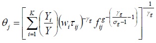 is an aggregate index of country
  is world output.27
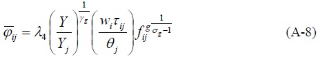
Substituting the price index and the productivity threshold into exports of an individual firm yields a bilateral export function that depends on productivity, trade costs (both fixed and variable), aggregate demand, remoteness, and input costs.

The bilateral export function for a firm with  indicates that, with lower trade costs, exports at the firm level increase through changes in the intensive margin. One obvious implication of the bilateral export function (A-9) is that the extent to which exports respond to changes in trade costs depends on the elasticity of substitution (
The sum of exports of firms with productivity  equals aggregate exports of product
 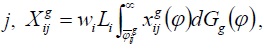 where
where

where
Analogously, aggregate imports of product  where
where

where
Substituting the productivity threshold, equation (A-8), into equations (A-10A) and (A-10B) yields

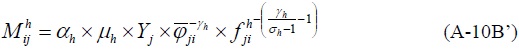
where  is the productivity of the least efficient firm in country
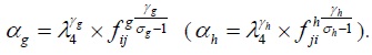
25)The numeraire good 0 is homogeneous, and good
26)
27)See
28)See 
29)The aggregate bilateral trade functions in
Appendix B. Instrumentation
In Table 1, the elasticity of total trade flows  with respect to comparative advantage
  for country
  for country
  which equals the extensive margin elasticity.
Given these elasticities, it is straightforward to retrieve information on  using the intensive margin elasticity
  and information on
  using the extensive margin elasticity
However, information retrieved above does not precisely represent unobservable costs. The intensive margin  is not proportional to
  in equation (4) since
  Nor is the extensive margin
  proportional to
  in equation (4) since
  So, the observable
  cannot exactly represent
  nor can the observable
  exactly represent
The inaccurate proxy problem, however, can be solved by applying multiple indicator IV methods (Wooldridge, 2010: 112-114). First,  can be used as the indicators of
  respectively. The relative position in the normalized unit costs of the source country against the destination country will affect the extensive and intensive margins of the source country. So will the relative advantage in the fixed trade costs of the source country against the destination country. Second,
  can be used as the second indicators of
  respectively. Since
  is correlated with both
  is correlated with
  only as shown in Table 1,
  can be used as an IV for
Appendix C.
Appendix Tables & Figures
Table C-1.
Korea’s Trading Partners in SITC 7 (2007-2013 average)

Table C-1.
Continued

Table C-1.
Continued

Table C-1.
Continued

Table C-1.
Continued

Notes: EM – extensive margin; IM – intensive margin; GL index – the Grubel Lloyd Index;  – GDP Partner/GDP Korea;
  – per capita GDP partner/per capita GDP Korea; FTA (years) – the number of years during which Korea and its trading partner maintain the common membership of an FTA. The data on GDPs are taken from the World Bank.
References
-
Bergstrand, J. H. 1990. “The Heckscher-Ohlin-Samuelson Model, the Linder Hypothesis and the Determinants of Bilateral Intra-Industry Trade,”
Economic Journal , vol. 100, no. 403, pp. 1216-1229.
-
Cameron, A. C. and P. K. Trivedi. 2010.
Microeconometrics Using Stata . (revised ed.) College Station: Stata Press. -
Chaney, T. 2008. “Distorted Gravity: The Intensive and Extensive Margins of International Trade,”
American Economic Review , vol. 98, no. 4, pp. 1707-1721.
-
Davis, D. R. 1995. “Intra-industry Trade: A Heckscher-Ohlin-Ricardo Approach,”
Journal of International Economics , vol. 39, no. 3-4, pp. 201-226.
- Davis, D. R. and D. E. Weinstein. 1996. Does Economic Geography Matter for International Specialization?. NBER Working Paper, no. 5706.
-
Davis, D. R. and D. E. Weinstein. 1999. “Economic Geography and Regional Production Structure: An Empirical Investigation,”
European Economic Review , vol. 43, no. 2, pp. 379-407.
-
Davis, D. R. and D. E. Weinstein. 2003. “Market Access, Economic Geography and Comparative Advantage: An Empirical Test,”
Journal of International Economics , vol. 59, no. 1, pp. 1-23.
-
Evenett, S. J. and W. Keller. 2002. “On Theories Explaining the Success of the Gravity Equation,”
Journal of Political Economy , vol. 110, no. 2, pp. 281-316.
-
Greenaway, D. and C. Milner. 1984. “A Cross-Section Analysis of Intra-Industry Trade in the UK,”
European Economic Review , vol. 25, no. 3, pp. 319-344.
-
Greenaway, D., Hine, R. and C. Milner. 1995. “Vertical and Horizontal Intra-Industry Trade: A Cross Industry Analysis for the United Kingdom,”
Economic Journal , vol. 105, no. 433, pp. 1505-1518.
-
Grubel, H. and P. Lloyd. 1975.
Intra-industry Trade: The Theory and Measurement of International Trade in Differentiated Products . London: Macmillan. -
Harrigan, J. 1994. “Scale Economies and the Volume of Trade,”
Review of Economics and Statistics , vol. 76, no. 2, pp. 321-328.
-
Helpman, E. 1987. “Imperfect Competition and International Trade: Evidence from Fourteen Industrial Countries,”
Journal of the Japanese and International Economies , vol. 1, no. 1, pp. 62-81.
-
Helpman, E. and P. R. Krugman. 1985.
Market Structure and Foreign Trade: Increasing Returns, Imperfect Competition, and the International Economy . Cambridge: MIT Press. -
Helpman, E., Melitz, M. and Y. Rubinstein. 2008. “Estimating Trade Flows: Trading Partners and Trading Volumes,”
Quarterly Journal of Economics , vol. 123, no. 2, pp. 441-487.
-
Hummels, D. and P. J. Klenow. 2005. “The Variety and Quality of a Nation’s Exports,”
American Economic Review , vol. 95, no. 3, pp. 704-723.
-
Hummels, D. and J. Levinsohn. 1995. “Monopolistic Competition and International Trade: Reconsidering the Evidence,”
Quarterly Journal of Economics , vol. 110, no. 3, pp. 799-836.
-
Krugman, P. R. 1979. “Increasing Returns, Monopolistic Competition, and International Trade,”
Journal of International Economics , vol. 9, no. 4, pp. 469-479.
-
Krugman, P. R. 1980. “Scale Economies, Product Differentiation, and the Pattern of Trade,”
American Economic Review , vol. 70, no. 5, pp. 950-959. -
Loertscher, R. and F. Wolter. 1980. “Determinants of Intra-Industry Trade: Among Countries and across Industries,”
Welftwirtschaftliches Archiv , vol. 116, no. 2, pp. 280-293.
-
Melitz, M. J. 2003. “The Impact of Trade on Intra-Industry Reallocations and Aggregate Industry Productivity,”
Econometrica , vol. 71, no. 6, pp. 1695-1725.
-
Weder, R. 1995. “Linking Absolute and Comparative Advantage to Intra-industry Trade Theory,”
Review of International Economics , vol. 3, no. 3, pp. 342-354.
-
Wooldridge, J. 2010.
Econometric Analysis of Cross Section and Panel Data . (2nd ed.) Cambridge: MIT Press.