I. INTRODUCTION

Living in the world where trade is becoming more active and the frequency and scale of capital movements are increasing among countries around the world, a proper understanding of the movements of the foreign exchange rate cannot be overemphasized. A diffusion process is used to model a variety of economic and financial variables. Among them, the exchange rate is an important example. Using a geometric Brownian motion (Black and Scholes, 1973) and (Merton, 1973) for the spot exchange rate, foreign currency option pricing formulas are derived by Garman and Kohlhagen (1983) and Grabbe (1983). Bollerslev and Zhou (2002) and Baldeaux et al. (2015) suggest a stochastic volatility model for the exchange rate. Researchers also combine jumps or regime-switching with diffusion models for the exchange rate, for example Akgiray and Booth (1988), Bates (1996), Swishchuk et al. (2014), and Goutte and Zou (2013). On the other hand, to explain the behavior of the exchange rate under a target zone regime, Krugman (1991) and Froot and Obstfeld (1991a) assume that the exchange rate follows a geometric Brownian motion.1 Alternatively, Froot and Obstfeld (1991b) use the Vasicek (Vasicek, 1977) model and Larsen and Sørensen (2007) employ the Jacobi diffusion and a generalization of the Vasicek model.

Univariate diffusion models employed by existing articles seem to be too simple to capture various features observed in the exchange rate. Their models do not seem to reflect the movements of the real data. Tucker and Scott (1987) provide empirical evidence contradicting the assumption of the geometric Brownian motion and constant elasticity of variance for the exchange rate.

Therefore, it is necessary to estimate general models with the exchange rate data to determine which model fits the data better. This paper considers five univariate different diffusion models including more general models than those proposed for the exchange rate in the literature to find a more appropriate model for each exchange rate. They are the Vasicek, CIR (Cox et al., 1985), CKLS (Chan et al., 1992), general drift and constant elasticity of volatility (hereafter GD-CEV), and general drift and general volatility (henceforth GD-GV) models. Choi (2009) generalizes Aït-Sahalia (1996)’s model by adding the third order term to the drift to get the latter two models. The GD-GV model has flexible drift and volatility functions and encompasses the other four models. We therefore expect it to explain the various characteristics of the exchange rate.

We use daily exchange rate quotations for 1 euro, 1 British pound and 100 Japanese yen in terms of US dollars. These three exchange rates are represented by USD/EUR, USD/GBP, and USD/100JPY, respectively. The data period of the first is January 4, 1999 to July 29, 2016 and the other two are January 6, 1986 to July 29, 2016.

The maximum likelihood estimation method is implemented to estimate the models. To do so, we must have the transition density function (TDF) or the logarithmic of the TDF (log-TDF) of a diffusion model. Although the true TDFs of the Vasicek and CIR models are known, those of the other three diffusions are unavailable. Hence the irreducible method developed by Aït-Sahalia (2008) is used to construct an approximate log-TDF.

In general, the TDF of a diffusion process is unknown. In order to address this problem, Aït-Sahalia (2002) first proposed to approximate the true TDF of a time-homogeneous univariate diffusion using Hermite polynomials. This has been generalized by Aït-Sahalia (2008) to obtain an approximate log-TDF of a time-homogeneous multivariate diffusion. Then, his work is extended to the cases of a time-inhomogeneous univariate diffusion by Egorov, Li, and Xu (2003), a time-inhomogeneous multivariate diffusion by Choi (2013) and Choi (2015), a time-homogeneous multivariate jump diffusion by Yu (2007), and a time-inhomogeneous multivariate jump diffusion by Choi (2019). Naming a few more related papers, they are Aït-Sahalia (1999), Li (2010), Bakshi and Ju (2005), Bakshi, Ju, and Ou-Yang (2006), Chang and Chen (2011), and Aït-Sahalia and Kimmel (2007, 2010).

Interestingly, of the five models, the CKLS model is sufficient to describe the USD/EUR exchange rate while the GD-GV model is the best of the 5 models for the cases of USD/GBP, and USD/100JPY. It appears that the volatility term plays a more important role in describing the dynamics of the exchange rate. Although we could not find any evidence of the mean-reverting property for the USD/EUR exchange rate, the USD/GBP, and USD/100JPY exchange rates show a tendency to revert to their long-run mean values as the exchange rate moves away from the mean. The volatility function of the USD/EUR exchange rate is increasing in the exchange rate. But the volatility functions of the USD/GBP and USD/100Yen exchange rates have a U-shape, which implies that the volatility has a minimum when the exchange rate around the long-run mean value and then it increases as the exchange rate moves away from the long-run average.

The estimation results reveal that different exchange rates behave differently. Therefore, when modeling exchange rates more care should be taken to ensure that the model reflects the dynamics of the real data. The results also imply that we may have to use a more general diffusion model than those proposed in the literature when developing economic theories for the behavior of the exchange rate and pricing foreign currency options or derivatives.

After showing data we discuss motivation of this research in the next section. We present five diffusion models we employ in this article and the estimation method in Section 3. Next section contains estimation results and how to interpret them. Then we conclude. Finally, more explanations about how to get an approximate log-likelihood function is in Appendix.

1)That is to say, the logarithm of the spot exchange rate is a Brownian motion with drift.

II. DATA AND MOTIVATION

Daily spot exchange rates expressed as the prices of 1 euro, 1 British pound and 100 Japanese yen in US dollars, respectively denoted by USD/EUR, USD/GBP, and USD/100JPY, have been obtained from Datastream. The sample period for the USD/EUR exchange rate is January 4, 1999 through July 29, 2016 and it is from January 6, 1986 to July 29, 20162 for the USD/GBP and USD/100JPY exchange rates. Descriptive statistics for these exchange rates are summarized in Table 1.

Figures 1A and 1B respectively exhibit daily exchange rates and daily changes in the exchange rate for the euro in terms of the US dollar (USD/EUR) for the period from January 4, 1999 to July 29, 2016. And a scattered plot of the daily changes in the USD/EUR exchange rate against the daily USD/EUR exchange rate over the same period is drawn in Figure 1C. Looking at Figures 1A and 1B, it is unclear whether or not the variability of the exchange rate is dependent on the level of the exchange rate. Figure 1C does not appear to reveal that changes in the exchange rate increase as the exchange rate moves away from the sample mean. Hence the USD/EUR exchange rate may not tend to revert to its long run mean level. However, it would be more appropriate to estimate proper models for the exchange rate and conduct statistical inference to investigate if we can find evidence for such behavior or not and to account for the movements of foreign exchange rates.

Analogously to Figures 1A through 1C, Figures 2A, 2B, and 2C display time series plots of the daily observations and its daily changes, and a scattered plot of the daily changes against the level, respectively, for the USD/GBP exchange rate between January 6, 1986 and July 29, 2016. For the same period, we have depicted similar graphs of the USD/100JPY exchange rate data in Figures 3A, 3B and 3C. It is difficult to tell if these two exchange rates have a tendency to return to their long-run mean values and there is any relationship between the exchange rate and its variability from a visual inspection of these graphs. In this article, we use continuous-time diffusion models that are capable of capturing the rich dynamics of exchange rates.

2)All the data available on July 29, 2016 were used. The data period for the USD/EUR exchange rate differs from the other two because the euro was introduced to world financial markets from January 1, 1999.

III. MODEL AND ESTIMATION METHODOLOGY

As discussed above, in the literature, researchers have adopted continuous time diffusions such as a Gaussian diffusion, the Vasicek model, and a geometric Brownian motion to model foreign exchange rates (Krugman, 1991) and (Froot and Obstfeld, 1991a; 1991b). However, their models have some limitations in describing real exchange rate data. Therefore, we need to adopt more general diffusion models which can capture various features of the exchange rate.

A diffusion model for a stochastic process X_t is expressed as a stochastic differential equation:

where μ(X_t; θ) and σ²(X_t; θ) are the infinitesimal mean and variance of the process X_t, respectively. Various specifications of the drift function, μ(X_t; θ) and the volatility function, σ(X_t; θ) are employed for many different economic and financial variables. One of the most popular variable used for diffusion process is the short-term interest rate. This paper estimates five diffusion models popularly suggested for short-term interest rates to describe and compare the dynamics of the USD/EUR, USD/GBP and USD/100JPY exchange rates. We consider more general models than the aforementioned diffusions utilized for the exchange rate in the literature and Table 2 provides all models examined in this paper. They are the Vasicek (Vasicek, 1977), CIR (Cox et al., 1985), CKLS (Chan et al., 1992), GD-CEV, and GD-GV models. Choi (2009) has added the third order term to the drift of Aït-Sahalia (1996)’s GD-CEV and general parametric models to get the GD-CEV and GD-GV models in Table 2, which are able to capture a steep drift when the state variable X_t is high.

The GD-GV model encompasses not only the other four diffusion processes but also most of univariate diffusion models proposed by researchers. It has flexible drift and volatility functions. The drift function is designed to examine whether or not the exchange rate has a tendency to return to its long-run mean level when the exchange rate is too high or too low. In addition, it allows the exchange rate to revert at different speeds depending on its values. Similarly, the general form of volatility function can reveal if the volatilities of the exchange rate are high when it is too big or too small. By estimating this general model and comparing it with the other four models, we can identify the best model that explains the movement of the exchange rate. At the same time, we can investigate distinct features of exchange rates from various aspects.

To ensure stationarity of diffusion processes some restrictions for the space of parameter values are derived following Aït-Sahalia (1996). Those conditions are

and

Conditions (1) and (2) are imposed for σ²(X_t; θ) to be positive in the neighborhood of the zero and infinity boundaries, respectively. Mean reversion of the drift term at high values of X_t is guaranteed by restriction (3) that makes infinity unattainable. Lastly, zero cannot be reached by condition (4).

In order to estimate the parameters of the models in Table 2 we adopt the maximum likelihood estimation method. Although a diffusion process is a continuous time model, data are observed only at discrete time points. Even so, we can carry out the MLE using discrete observations, x_iΔ, i = 0,1, … , n, where Δ is the time difference between two consecutive observations. Because we have daily time series data Δ = 1/252.3

To do the MLE we must know the joint probability density function of all variables,

which can be rewritten as

by the Bayes’ rule. Thanks to the Markov property a diffusion model this can be further simplified to

Ignoring the initial observation, the log-likelihood of the data is

Therefore if we know the transition density function (TDF), p(x|x_o; θ) or the log-likelihood function ln[p(x|x_o; θ)] = l_X(Δ, x|x_o) we can find the maximum likelihood estimates of θ by maximizing (5).

However, the true TDF of a diffusion process is unknown in general. The true TDFs of the Vasicek and CIR models are known while those of the other more general models in Table 2 are unavailable. Aït-Sahalia (2002) has done a pioneering work of finding an approximate TDF (ATDF) of a time-homogeneous univariate diffusion model explicitly by exploiting Hermite series expansion. Then he developed a way to obtain a closed-form approximate log-TDF of a time-homogeneous multivariate diffusion process in Aït-Sahalia (2008). We make use of the method from Aït-Sahalia (2008) to derive log-likelihood expansions of all models we consider in this article.

Let us briefly explain how to get an approximate log-TDF of a time-homogeneous univariate diffusion model. A diffusion process is said to be reducible if it can be transformed into a unit diffusion model where the volatility is an identity matrix. If it is not reducible we call it irreducible. Univariate diffusion is reducible, but not all multivariate diffusions are reducible. Aït-Sahalia (2008) suggested two different methods of obtaining log-likelihood expansions for reducible and irreducible cases. Although all of our models are univariate and reducible, we cannot adopt the reducible method as there does not exist a closed-form formula of the transformation4 by which the GD-GV model can be converted into a unit diffusion. Therefore the irreducible method is applied to acquire approximate log-likelihood functions.5 For more explanations about the irreducible method please see Appendix.

3)For the weekly and monthly data Δ= 1/52 and Δ= 1/12, respectively. Moreover, if the time differences of two successive data are not equal, for instance due to missing observations, the values of Δ can be adjusted accordingly.

4)Such a transformation is called Lamperti transformation.

5)We could have used Hermite series expansion proposed by Aït-Sahalia (2002) since all of our models are time-homogeneous univariate cases. Hermite series expansion is a Taylor series expansion of the true TDF in the state variable x and Δ, which is actually equivalent to the log-likelihood expansion obtained by the irreducible method. The true TDFs of the Vasicek and CIR models are available and the reducible method can be used for the CKLS and GD-CEV models. Nonetheless, the irreducible method is used to get approximate log-likelihood functions of all models for the sake of consistency. Moreover, those approximations perform fairly well comparing to the true TDF. See Aït-Sahalia (2002, 2008) for more details.

IV. ESTIMATION RESULTS AND DISCUSSION

Tables 3, 4 and 5 tabulate estimation results of the USD/EUR, USD/GBP and USD/100Yen exchange rates, respectively. ML estimates of the parameters with standard errors in parentheses, maximum log-likelihood values, p-values of the likelihood ratio (LR) test to compare the other four models with the GD-GV model and information criteria AIC and BIC6 are presented in each table. Figures 4 through 6 are for the USD/EUR, USD/GBP and USD/100Yen exchange rates in order. For each of these exchange rates, using the estimates of the parameter and covariance, the first and second columns of Figures 4, 5, and 6 respectively draw drift and the volatility functions and their 95% confidence bands for all models. Interestingly, our findings show that those three exchange rates behave differently.

The CKLS model is sufficient to describe the USD/EUR exchange rate, while the GD-GV model is preferred over the other four models in the cases of USD/GBP and USD/100Yen. There is no evidence of mean reversion for the USD/EUR exchange rate, but the USD/GBP and USD/100Yen exchange rates are found to have such a property. When it comes to the volatility, all parameters of the volatility function are statistically significant at the usual level in all exchange rates. It is very interesting that the volatility functions of the USD/GBP and USD/100Yen exchange rates have a U-shape, compared to having a monotone increasing volatility function for the USD/EUR case.

For the USD/EUR exchange rate, of the 5 models, the CKLS model is found to be sufficient to explain the dynamics of the data. The Vasicek and CIR models are rejected while the CKLS and GD-CEV models cannot be rejected when tested against the GD-GV model. The CKLS model is preferred over the other 4 models based on the information criteria, AIC and BIC.

None of the parameters of the drift functions in any models are significantly different from zero. Looking at drift functions and their 95% confidence bands, all of the confidence bands include the x-axis, which illustrates that the drift function is statistically indistinguishable from zero.

On the other hand, all parameters of volatility functions except the GD-GV case are statistically quite significant. The second column of Figure 4 tells that the volatility is increasing in observed exchange rates.7 These imply that the volatility plays a more important role in describing the dynamics of USD/EUR exchange rates than the drift.

Unlike the USD/EUR case, the GD-GV model is the best as the other four models are rejected in the LR test even at the 1% significance level for the USD/GBP exchange rate. Besides, the AIC and BIC values of the GD-GV model are the smallest.

We have also found some evidence of mean reversion in the Vasicek, CIR and CKLS models that have a linear drift function. In these models all of the drift parameters are statistically significant and the 95% confidence bands do not contain the x-axis at high and low exchange rates as can be seen in Table 4 and Figure 5. Noticeably, when the USD/GBP exchange rate goes away from 1.6 it demonstrates the mean reverting behavior. However, we do not observe this phenomenon in the GD-CEV and GD-GV models where we employ a more general nonlinear drift function.

In all models, the parameters of the volatility function are all statistically significant at the 1% level. This means that the volatility of the USD/GBP exchange rate varies with the exchange rate. More interestingly, the volatility function of the GD-GV model is U-shaped.

The volatility of the USD/GBP exchange rate has a minimum when the exchange rate is about 1.6 and increases as it moves away from 1.6. Note that the sample average of the USD/GBP exchange rate is 1.64.

Similarly to the USD/GBP case, the GD-GV model describes the dynamics of the USD/100Yen data better than the other four models because the p-values of the LR test for the other four nested models against the GD-GV model are all very small. And in terms of the information criteria AIC and BIC, the GD-GV is also preferred over the other four models.

All of the drift parameters for the Vasicek, CIR, and CKLS models and some parameters of the drift function for the GD-CEV and GD-GV models are statistically significant at the 1% or 5% significance level. Even so, we need to draw the drift function with confidence bands to see if the USD/100Yen exchange rate tends to revert to its long run mean. The first column of Figure 6 shows that the 95% confidence bands do not include x-axis when the exchange rate is high or low in all models, which indicates that the USD/100Yen exchange rate exhibits the mean reverting property when it moves away from 0.9. It is worth mentioning that the sample mean of the USD/100Yen is 0.89.

All of the volatility parameters are statistically significant at the 1% or 5% level. Checking the second column of Figure 6, in the cases of CIR, CKLS, and GD-CEV, the volatility is a monotone increasing function of the exchange rate. However, the volatility of the GD-GV model decreases at first and then begins to increase as the exchange rate passes 0.6. This result is analogous to that of the USD/GBP case, but the turning point is slightly smaller than the sample average in this case.

What we can learn from our estimation results is that different exchange rates behave differently. As is the case for the USD/EUR exchange rate, more general models do not necessarily perform better. However, our findings show that we need to use a more general diffusion model than those assumed in the existing literature to explain and describe the dynamics of the exchange rate. Even if we have not compared diffusion models in terms of developing economic theories for the movements of the exchange rate and pricing foreign currency options and derivatives, we might have obtained distinct results in these areas if we have used a more general diffusion process. This can be an interesting future research topic.

6)The AIC is proposed by 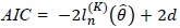Akaike (1973) is and the BIC suggested by Schwarz (1978) is is the maximized value of the log-likelihood of a model and d is the number of parameters in the model. The model with the smallest AIC or BIC value is preferred.

7)It is not the case for the Vasicek model just because it has a constant volatility.

V. CONCLUSION

This paper compares three different foreign exchange rates by estimating five different univariate diffusion models. Those exchange rates are daily quotations in US dollars for 1 euro (USD/EUR) from January 4, 1999 to July 29, 2016 and 1 British pound (USD/GBP) and 100 Japanese yen (USD/100Yen) from January 6, 1986 to July 29, 2016. The Vasicek (Vasicek, 1977), CIR (Cox et al., 1985), CKLS (Chan et al., 1992), GD-CEV, and GD-GV (Aït-Sahalia, 1996) and (Choi, 2009) models are adopted for the estimation of each exchange rate. We employ the maximum likelihood estimation method to estimate these models. In doing so, the irreducible method (Aït-Sahalia, 2008) is applied to approximate the true but unavailable log-transition density function of the diffusion process.

As a result of estimation, the most general model (GD-GV) performs the best for the USD/GBP and USD/100JPY exchange rates while the CKLS model is sufficient to describe the USD/EUR data based on the likelihood ratio test and the information criteria, AIC and BIC. Even if we could not find any evidence for the existence of mean-reversion for the USD/EUR case, the USD/GBP and USD/100JPY exchange rates illustrate a tendency for them to return to their long-run average values when the exchange rates are relatively high or low. The volatility function of the USD/EUR exchange rate is increasing in the exchange rate while the volatility functions of the USD/GBP and USD/100Yen exchange rates have a U-shape.

Our findings indicate that different exchange rates behave differently and more general models do not necessarily fit the data better. Therefore, we need to choose a model that can reflect and explain the movements of the exchange rate case by case. We also learned that we need a more general diffusion model for the exchange rate than those suggested in the literature. Studying implications of our estimation results for developing economic theories for the movements of the exchange rate or pricing foreign currency options or derivatives would be an interesting future research topic. Moreover, estimating a jump diffusion model or a regime-switching diffusion model or multivariate diffusion models using the exchange rate data would be another nice future work to do. As explained in Section 1, researchers have developed how to approximate the TDF or log-TDF of a jump diffusion or a multivariate diffusion models. Moreover, if we want to use a stochastic volatility model for the exchange rate, the volatility factor is unobservable. In this case, we can use high frequency data to calculate realized volatilities or exploit option prices to obtain implied volatilities. These can be used for the latent variable. Finally, some researchers employ models for a logarithm of exchange rates. We could have considered diffusion models in a logarithm of exchange rates rather than in levels. In fact, it is possible to find the relationship between two diffusion models in a log of exchange rates and in levels using the Itô lemma. Furthermore, because a logarithmic function is monotone increasing; we expect to get qualitatively quite similar results when using a log of the exchange rate.

The key idea of the irreducible method is to postulate the form of K-th order log-likelihood expansion as the one from the reducible method as follows:

Then, using the fact that l_X(Δ, x|x_o; θ) satisfies the Kolmogorov forward partial differential equation (PDE),

if we put (6) in (7) and equate the same order terms of Δ we end up getting the following PDEs for the coefficients of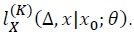

and when k ≥ 1

where

and for all k ≥ 2

These PDEs of 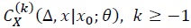cannot be solved analytically when an explicit form of the Lamperti transformation is unobtainable as is the case for the GD-GV model. In this case, Aït-Sahalia (2008) suggested to Taylor expand μ(x; θ), and σ(x; θ) in x about x_o in each PDE and to compare both sides of the PDE to come by the coefficients of the Taylor expansion.

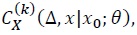
To make the same approximation error as 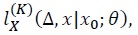each coefficient 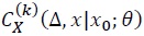needs to be Taylor-expanded up to 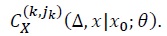j_k-th order and we denote it by If the approximation error is of order 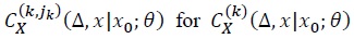O_p(Δ^K+1) we need to set j_k = 2(K - k + 1) for each k. For example, when K = 2, only five coefficients are required and j_-1 = 8, j_o = 6, j₁ = 4 , j₂ = 2, j₃ = 0. Substituting in equation (6),

In obtaining it has to be done from k = −1 sequentially because all of the subsequent coefficients are dependent on the previous coefficients. Besides, we must attain the Taylor expansion from the lower order term since higher order terms hinge upon the lower order terms.

Using the approximate log-likelihood expansion (8) we maximize

to get the approximate MLE, which has been proved to behave just like the true MLE theoretically and by Monte Carlo simulation studies.