
Corruption, Taxation and the Impact on the Shadow Economy


1
Faculty of Economics and Administration, Masaryk University, 601 77 Brno, Czech Republic
2
School of Business Administration, Silesian University, 733 40 Karviná, Czech Republic
3
Department of Economics and Economic Policy, PRIGO University, 736 01 Havířov, Czech Republic
4
Department of Business Economy and Law, PRIGO University, 736 01 Havířov, Czech Republic
*
Author to whom correspondence should be addressed.
Economies 2021, 9(1), 18; https://doi.org/10.3390/economies9010018
Submission received: 22 December 2020
/
Revised: 19 January 2021
/
Accepted: 28 January 2021
/
Published: 4 February 2021
(This article belongs to the Special Issue Impact of Corruption on the Economy)
Abstract
:While assessing the economic impacts of corruption, the corruption-related transmission channels which influence taxation as such have to be duly considered. Taking the example of the Czech Republic, this article aims to evaluate the impacts corruption has on the size of the shadow economy as well as on the individual sources of long-term economic growth, making use of a transmission channel through which corruption affects the tax burden components. Using the method of an extended DSGE model, it confirms the initial assumption that an increase in perceived corruption supports the shadow economy’s growth, but at the same time, it demonstrates that corruption and especially its perception has a significantly different effect on two key areas—the capital accumulation and the labour force size. It further identifies another sector of the economy representing taxes which are prone to tax evasion while asserting that corruption has a much more destructive effect on this sector of the economy, offering generalized implications for other post-communist EU member states in a similar situation.
JEL Classification:
A10; H20; E601. Introduction
Corruption is a phenomenon probably as old as mankind itself. The negative and sometimes even devastating effects it has on most areas of society and economy are far-reaching and have been widely described by numerous researchers. As far as the economic impacts are concerned, the consequences related to the investment impact, capital accumulation, labour force and the relevant economic growth are of particular importance. Meanwhile, it is essential to underline at an early stage that it is not only the erosion of these variables that undermines the economic level and social well-being, but it is also the corruption-related transmission channels that significantly impact taxation as such. Quite commonly, economic agents perceive an even higher taxation level, yet without significant tax uncertainty, as a positive trait which usually translates into a stable and transparent surrounding institutional environment. Consequently, even with a relatively high tax burden, an economy may find itself in good shape given that the corruption level, lobbying and non-transparent behaviour is low. This is intuitively visible, for example, in the Scandinavian countries. In this regard, we must not underestimate the negative effects a corrupt and non-transparent environment has on increasing the share of the shadow economy while adding up all the negative consequences to this.
A large part of the new post-communist European Union member states is to some extent affected by the negative consequences related to corruption and conflict of interest of strong lobby groups or individuals. Therefore, the European Union is, as a whole entity, facing significant challenges in the areas of the rule of law and transparency, which can be generally attributed to the post-communist EU member states. This results in the current stalemate concerning the approval of the EU budget. It is our belief that by selecting the example of Czech Republic as a representative sample among these countries, our research can draw pertinent conclusions and can be further used for valid approximation of the results and their broader application to other European states. Indeed, since the Czech Republic shows similar institutional parameters as other post-communist members and because of its central position on the border between former and new EU member states, it may serve as a convenient example in either confirming or refuting the hypothesis of the negative impact corruption has on the side of the shadow economy as well as on individual economic factors that are being considered as sources of long-term economic growth. The Czech Republic is a country where the concept of fighting corruption is rhetorically present on all levels of the public space. Similarly, anti-corruption rhetoric accounts for a regular subject in pre-election debates and public debates in general. Despite that, corruption is still perceived as a relatively frequent practice in the country, and the situation in other post-communist EU countries is rather similar in this regard. To elaborate, the local Transparency International branch which deals with corruption issues is very active in the Czech Republic. At the same time, its chairman is the only representative from the EU post-communist countries within the Board of Directors’ supreme body.
The aim of this article is to evaluate the impacts corruption has on the size of the shadow economy as well as on the individual sources of long-term economic growth. We shall make use of a transmission channel through which corruption affects the tax burden components. The conclusions from the selected Czech Republic’s benchmarks are then used as the basis for the general assessment of the (especially post-communist) members of the European Union. The implications arising from this article may be thus used by economic policymakers not only within the individual countries but especially within the implementation processes at the level of EU institutions.
The extended DSGE model developed by Orsi et al. (2014), which considers both official and shadow economies, shall be used. Given the key role which corruption impact transmission plays via perceiving individual components of the tax burden, this model shall be significantly expanded to address the separate impact that individual components of tax burden have in the tax mix, including social security contributions.
2. Literature Review
Concerning the definition, in this article, corruption is to be understood in accordance with the Transparency International’s definition which stands for “an abuse of entrusted power for private gain” (Transparency International 2020b). Being aware of other definitions that can be traced in scientific literature and which often take into account the individual attributes of corruption according to how corruption is perceived, we would like to note the following: Nye (1967) ranges among the best-known and most frequently cited authors to have defined corruption. He sees it not only as the result of a conflict between the private and the public sector but as “any behaviour violating the rules in order to increase private influence”. Additionally, the issue of corruption is frequently associated with economic impacts, but it is also dealt with by the humanities, which view it, for example, as deviant or pathological behaviour or a form of social disorganization (Frič 2001).
The practical manifestation of corruption and its implications are, however, far more complex. They are related to the transmission channels through which corruption takes place. It is also necessary to consider, particularly in relation to national legal systems, what conduct falls under “corrupt” and what conduct may establish criminal liability. Notably, it seems crucial to acknowledge the importance of how corruption is perceived, as it is not the actual, but mostly the perceived corruption, which is transmitting into the perception of the tax burden and the tax rates (see Torgler and Schneider 2009; Schneider 2011), and as is assumed later in this article, too.
Despite the fact that the share of the shadow economy has been declining over time, according to Medina and Schneider (2018), corruption forms a key factor impacting the transfer of some activities to the informal, or rather shadow economy. A study by Dreher and Schneider (2010) reflects how closely corruption and the shadow economy are linked. According to their analysis, corruption and the shadow economy can be seen as substitutes in developed high-income countries, whereas in countries with a low per capita income, they may be perceived as complementaries, that is, as complementary economic phenomena. These conclusions are more or less confirmed by a subsequent study by Borlea et al. (2017), which demonstrated, based on an analysis carried out in the EU countries in the 2005–2014 period, a positive relationship between corruption and the shadow economy. As a matter of fact, higher corruption levels lead to a higher shadow economy share, and according to this specific study, almost one-fifth of the EU countries’ GDP can be attributed to the shadow economy. In addition, Shahab et al. (2015) concluded in their analysis that the relationship between corruption and the shadow economy depends on the size of corruption. With the perceived level of corruption growing, its positive relationship with the shadow economy becomes more evident.
Moreover, the relationship between corruption and taxation, which can be described as multifaceted, appears to be significant. Liu and Feng (2014) focused on the relationship between corruption and direct/indirect taxes. They concluded that countries relying more heavily on direct taxes tend to enjoy a lower level of corruption, while countries with more complex tax systems tend to have a higher level of corruption, precisely because a more complex tax system can be controlled less properly. Tax morale, the quality of institutions and their impact on the shadow economy are also related to this, as reported by Zubaľová et al. (2020), Kirn et al. (2019), or Torgler and Schneider (2009) who, based on cross-sectional analysis, concluded that reducing corruption helps eliminate the effort to move to a shadow economy.
Corruption or, at its best, lobbying already becomes evident in the constitution of tax laws where certain groups of agents are often favoured without showing any obvious logic. Currently, there is a worldwide discussion going on, for example, related to tax advantages provided for technology giants as far as income tax is concerned. The suspicion of a sub-optimally set tax system cannot be avoided even when it comes to the key value-added tax (VAT) and the setting of a reduced tax rate for certain groups of products and services or, for example, with the exemption of financial services.
Corruption manifests itself when it comes to applying tax laws, especially tax administration ones, in many areas. This refers both to the tax audit itself and to potential subsequent criminal proceedings. Several authors (Fjeldstam 1996, 2003; Buehn and Schneider 2009; Kaufmann 2010; Ivanyna et al. 2010; Ghosh and Neanidis 2011) state that corruption serves as a mean of tax evasion.
Corruption can therefore affect the taxpayer in a way that non-payment of taxes not only becomes legally intangible but also morally acceptable. Significant demotivation on the part of the taxpayer therefore arises, including a legally non-conforming behaviour. In particular, those taxes which are prone to tax evasion according to the tax theory, such as the excise tax, are not properly collected due to corruption. As a consequence, the official economy’s share is declining in favour of the shadow economy, as evidenced by studies by Borlea et al. (2017), Kaufmann (2010), or Hoinaru et al. (2020), who, based on their analysis, postulate that the negative effects of corruption and the shadow economy are higher in high-income countries than in the case of low-income countries. These conclusions reveal that the transmission channel of the impact corruption has on economic fundamentals and the shadow economy, and which is conditioned by perceiving an efficient tax burden by the taxpayer himself, is of essential importance.
3. Research Design and Methodology
Based on the literature review, we formulate a hypothesis that corruption negatively affects tax morale and thus the extent of the shadow economy. If this hypothesis is confirmed, then we can further assume that the growing importance of the shadow economy will also mean a shift in activities related to the key factors of economic growth from the official to the shadow economy and the associated distortion effects. In other words, we assume that through the channel of tax evasion, corruption leads to a shift of activities including labour size and capital accumulation from the official to the shadow economy, however, not necessarily to the same extent.
This article thus examines the links between corruption, taxation and the shadow economy. From a methodological point of view, it uses a dynamic stochastic general equilibrium model (the DSGE model), based on microeconomic variables and capturing all major sectors as a system. The Orsi model (Orsi et al. 2014), which already includes the shadow economy and, in general, direct and indirect taxes, is significantly extended to the elementary level of individual types of taxes in the tax mix. A comprehensive approach in the field of tax policy modelling methodology can be found in the work of Auerbach (2017).
The DSGE model, into which corruption through tax rates is integrated, is a comprehensive equilibrium model that is able to examine the short-term dynamics of model variables and simulate economic shocks. The unique way of integrating corruption into the DSGE model is not very common in the literature when examining its effects, despite the fact that, currently, DSGE modelling is one of the mainstream ways of describing economic behaviour. Corruption is usually included as an explanatory variable mainly in long-term regression growth models, in which individual variables (direction of action and quantitative influence) are examined, where, however, not all interrelations resulting from optimization behaviour can be affected. In these models, it is also problematic to affect links in shorter periods.
Estimates and presentations of the results of the DSGE model we construct are based on the standard and usual structure presented in recognized journals by leading authors in the field of DSGE modelling, such as Pappa et al. (2015), or Solis-Garcia and Xie (2018). Lindé’s (2018) work is crucial for the current debate on the usefulness of the DSGE approach for economic policy.
The starting point for modelling the impact that corruption has on our economy is a calibrated DSGE model that considers the shadow economy sector, as based on the model described in Orsi et al. (2014). However, for the purposes of the present study, the model was substantially modified in analogy to the approach described in Kotlán et al. (2019) so as to include tax rates structurally corresponding to the current tax mix in the researched economy. However, in contrast to this work, attention is given to the implementation of transmission mechanisms of the factor reflecting how corruption is being perceived in the tax area. A key aspect of the methodology used, however, remains the modification and full-scale derivation into a two-sector model of companies including the production of goods that are subject to the value-added tax (VAT) only, and goods that are also subject to the excise taxes. This aspect was further reflected through the modified consumption function which considers both types of goods.
There are three types of representative agents included in the model: companies, households and government. Tax revenues are composed of personal income taxes (), social security contributions (), corporate tax (), withholding tax (dividend tax, ), of the value-added tax (), excise taxes () and the fines imposed for government-controlled and detected activities of companies in the shadow economy ( when XXX is defined as a surcharge on the assessed tax liability).
Corruption is integrated into the model through the effect it has on each component of the effective tax rate within a specific partial tax. This mechanism corresponds to the approach shown in Born and Pfeifer (2014), or Kotlán et al. (2019), where it is incorporated as a multiplicative term to the corresponding stochastic components of the model. In our case, the corruption indicator is common to all stochastic tax rates, differing only in the relative weights of their impact on the resulting perceived tax rate.
Companies and households can carry out their activities both in the official economy sector (the relevant variables will be marked with a superscript ), and in the shadow economy sector (referred to using the superscript ). In every period, companies are facing the risk of being controlled by the government. The consequence of the inspection is that, in addition to unpaid taxes, companies furthermore must pay the relevant fines. Similarly, households are trying to avoid their tax obligations by offering part of their work (and capital renting) to the shadow economy sector. The short-term economy dynamics are affected by shocks in the productivity of individual companies’ production technologies, shocks in household preferences, investment shocks and fiscal shocks.
Due to the introduction of specific goods subject both to VAT and excise taxes, we shall consider two production areas. The first area refers to producing normal goods (not subject to excise tax, variables related to this area are indicated by superscript 1), the second area refers to producing specific goods subject to excise taxes (activities in this area are indicated by superscript 2. Every company is using work in the official sector of the economy, , and capital, , for producing final goods and using technologies described by Cobb-Douglas production functions:
where the parameters , , and represent temporary technological shocks. The XXX stands for a permanent technological shock affecting exclusively labour force and having the character of a deterministic trend , where XXX can be identified with the growth of the potential product of the economy. Each unit of companies’ net income (defined as the difference between final output, labour costs and leased capital) is taxed using a stochastic corporate tax , which is directly proportional to the perceived corruption factor referring to the corporate tax, , where represents a relative weight with respect to the overall perception of the corruption indicator, . Thus, the increase in perceived corruption generally raises the effective tax rate, implicitly in line with the Baklouti and Boujelbene (2019) mechanism, where the increase in perceived corruption is identified as a higher willingness to enter the shadow economy, linked with declining tax revenues and compensation by further raising tax rates. Subsequently, in the case of some companies, , the profit after taxation, distributed as dividends, is taxed according to the withholding tax , which is again directly proportional to the factor of perceived corruption as far as corporate tax is concerned, .
Companies may hide part of their production to avoid tax liability. Thus, companies can produce part of the output within the shadow economy sector making use of Cobb-Douglas production functions analogous to Equation (1), where the index for the shadow economy and the definition and as temporary technological shocks is used. Due to the specific nature of the value-added tax and excise taxes, which directly affect the price of goods and services, we shall assume possible differences in the products of the official and shadow economy. Assuming perfectly competitive markets, companies shall be treated as price recipients, while prices on the official market (excluding taxes) and on the shadow economy market may differ reflecting, for example, a risk premium.
Labour and capital markets are also perfectly competitive. Consequently, companies pay interest on renting capital or rather . On the official market, labour costs are determined by the wage rate per labour unit , increased by the social insurance stochastic tax rate (including corruption factor ). Labour costs in the shadow economy are determined merely by the wage rate .
In order to prevent tax evasion, the government uses a control process in each period, where each company is facing the probability of , or in individual parts of its activities within the shadow economy that their potential business in the shadow economy will be investigated and revealed. In this case, companies are forced to tax their net output in the shadow economy valued at the usual prices of the official economy at the tax rate increased proportionally by penalties and additionally, they have to pay the excise taxes and value-added tax, increased proportionally by penalties or . We neither consider additional taxation of profits resulting from the withholding tax nor an additional assessment of social security contributions rates.
As part of their decision-making, households are trying to maximize the benefits of consumption in the economy of manufactured goods, while offering their work and available capital to companies to obtain these values. A representative household is striving to maximize its utility function:
where represents the inverse value of the interstitial elasticity of the substitution, is a subjective discount factor, represents a parameter of preferences for the benefit of acquiring goods in the shadow economy (including e.g., the cost of leisure time to find a given market), which provides that the goods’ prices in the official and shadow economy can differ. The parameter represents an inverse elasticity of substituting the consumption of individual goods generated by shadow economy, and are preference parameters referring to benefits from work activities. The and parameters reflect the inverse elasticities of the substitution of the total labour supply and the labour supplied to the shadow economy. represents a transient shock in labour supply affecting the marginal rate of substitution between consumption and leisure.
As a result of considering two types of goods, represents a consumption index corresponding to the standard CES specification of the utility function, in the following form:
where is the share of consumption of specific goods in total consumption, and expresses the elasticity of substitution between the two types of goods, while in the basic consumer index, the consumer does not distinguish qualitatively between the consumption of given goods obtained from the official or shadow sector of the economy. Households offer their work to companies in both parts of the economy, just as they are renting their capital. Capital stock, , is evolving in time according to the following rule:
where indicates investment throughout time and represents the rate of capital depreciation. The transfer efficiency of final goods into physical capital is a random variable determined by transient shocks . The capital is homogeneous, and a household can decide at any time which portion it will lend to companies within the official sector of the economy (amounting to ) and how much it assigns to the shadow economy sector (in volume ). Households can avoid paying household income tax when shifting their labour and capital supply from the official sector to the shadow economy, where income from the shadow economy amounting to is not subject to income tax at a given rate of , including the corruption perception factor . Given these assumptions, the budgetary household constraint at any given time is determined as:
with the capital provided to both sectors of the economy fulfilling the condition of
The value-added tax rate, , and the excise tax rate, , reflect factors of corruption perception , or .
The government sector is modelled according to the government adjusting at all times tax rates to finance a given volume of government consumption, .
where the first item on the right side of the equation gradually represents the total fiscal income from personal income taxation, , from taxation of corporate profits, , from withholding tax on profit sharing, , from social security contributions, , from the value-added tax, , and excise taxes, . Government revenues represent tax revenues and revenues from additional tax assessments and imposed penalties. The values of steady-state tax rates shall be further calibrated as averages of observed statutory tax rates in individual tax categories.
Exogenous stochastic processes (productivity shocks, fiscal shocks, or shocks in tax rates) and other exogenous variables shall be modelled as independent autoregressive processes similar to Orsi et al. (2014), or Kotlán et al. (2019). The non-linear form of the model expresses the relevant indicator in a technically similar way as in Born and Pfeifer (2014), that is, multiplicatively to the corresponding stochastic components of the model. The model was log-linearized for the purposes of further simulations.
4. Data
Annual as well as quarterly data covering the period from the first quarter of 2002 until the fourth quarter of 2019 were used to calibrate the steady states of the parametrized linearized model and part of the model parameters. The time series used (with relevant source included in brackets) and their model counterpart (following a corresponding transformation) are as follows:
- Gross fixed capital formation (in CZK mio. CZK at constant prices, quarterly data (CNB 2020), .
- Consumer price index, CPI, basic index with a reference value of 100 for 2005, seasonally adjusted by the X13-ARIMA procedure, quarterly data, ARAD (CNB 2020), .
- Real wage, expressed via the nominal wage in CZK for the Czech Republic using the consumer price index, seasonally adjusted by the X13-ARIMA procedure, quarterly data (CNB 2020), .
- Personal income tax (dependent activity, return), collection of national tax revenues in CZK billion, annual data, ARAD (CNB 2020), .
- Corporate income tax, collection of national tax revenues in CZK billion, annual data, ARAD (CNB 2020), .
- Personal income tax (withholding tax), collection of national tax revenues in CZK billion, annual data, ARAD (CNB 2020), .
- Social security and health insurance premiums, selected indicators of the state budget in CZK billion, annual data, ARAD (CNB 2020), .
- Value-added tax, collection of national tax revenues in CZK billion, annual data, ARAD (CNB 2020), .
- Excise taxes, collections of national tax revenues in CZK billion, annual data, ARAD (CNB 2020), .
- Production at constant prices according to NACE codes, in CZK ths., 2015 constant prices, annual data (CZSO 2020), . Categories 6 (oil and gas extraction), 11 (beverage production) and 12 (tobacco production) were chosen as representatives of the sectors being subject to excise tax. This is an approximation in the sense that from the point of view of oil and mineral oil production, the Czech Republic is an importer of these raw materials. However, given the dynamic development within this industry, these sectors can be considered representative.
- Hours worked according to NACE codes, annual data (CZSO 2020), .
- Number of inspections and audited entities-VAT and corporate income tax, annual data (MFCR 2020), . The detection probability is set as the average value of the number of inspections and the number of controllable entities for the case of corporate income tax inspection (probability of detection within industry 1) and for the case of VAT inspection (probability of detection in industry 2).
- Corruption Perception Index (CPI), annual data (Transparency International 2020a), .
We are aware that there exist other indicators that are used to measure corruption. These focus mainly on corruption experiences, such as the World Bank Enterprise Survey. This is data collected directly from companies in the country, and one indicator is the percentage of companies that consider corruption to be the biggest obstacle in their business (World Bank 2020). However, this survey is not carried out even annually, but in much longer periods of time. For example, data for the Czech Republic are available only for the years 2009, 2013 and 2019, which is insufficient for the purposes of our analysis, given the selected time period (2002–2019) and the method of estimating the model. Another one of the composite indices that is compiled and contains data on corruption is the International Country Risk Guide from PRS Group. Corruption is one of the components of the overall index and, as in the case of World Bank, it focuses on corruption experiences in the form of excessive patronage, nepotism, job reservations, “favour-for-favours”, secret party funding, etc. (PRS Group 2020). The difference between the perception of corruption and real corruption (experience with it) is described, for example, in papers by Olken (2009), or Donchev and Ujhelyi (2014). These authors agree that distinguishing corruption perception and experience can, indeed, affect the results of the analyses performed and, in particular, their interpretation. Nevertheless, we use the Corruption Perceptions Index because both indices focused on corruption experiences are compiled exclusively on the basis of companies’ experience, while CPI data are obtained not only from company managers but also from public administration representatives. This fact will enable more meaningful and precise integration into the DSGE model through the impact of corruption on individual types of tax rates, which include all taxes of the tax mix, that is, not just corporate taxes.
Annual time series were interpolated into quarterly time series using the so-called cubic Hermitian interpolation polynomial method. Based on the calibrated parameter values as well as the values of steady states of exogenous quantities, the steady states of endogenous quantities were calculated within the non-linear form of the model using the Dynare toolbox version 4.6.1 (Adjemian et al. 2011). The observed variables enter the model as centred growth rates. Steady states are indicated by a comma above the variable symbol in the following tables.
5. Empirical Results and Discussion
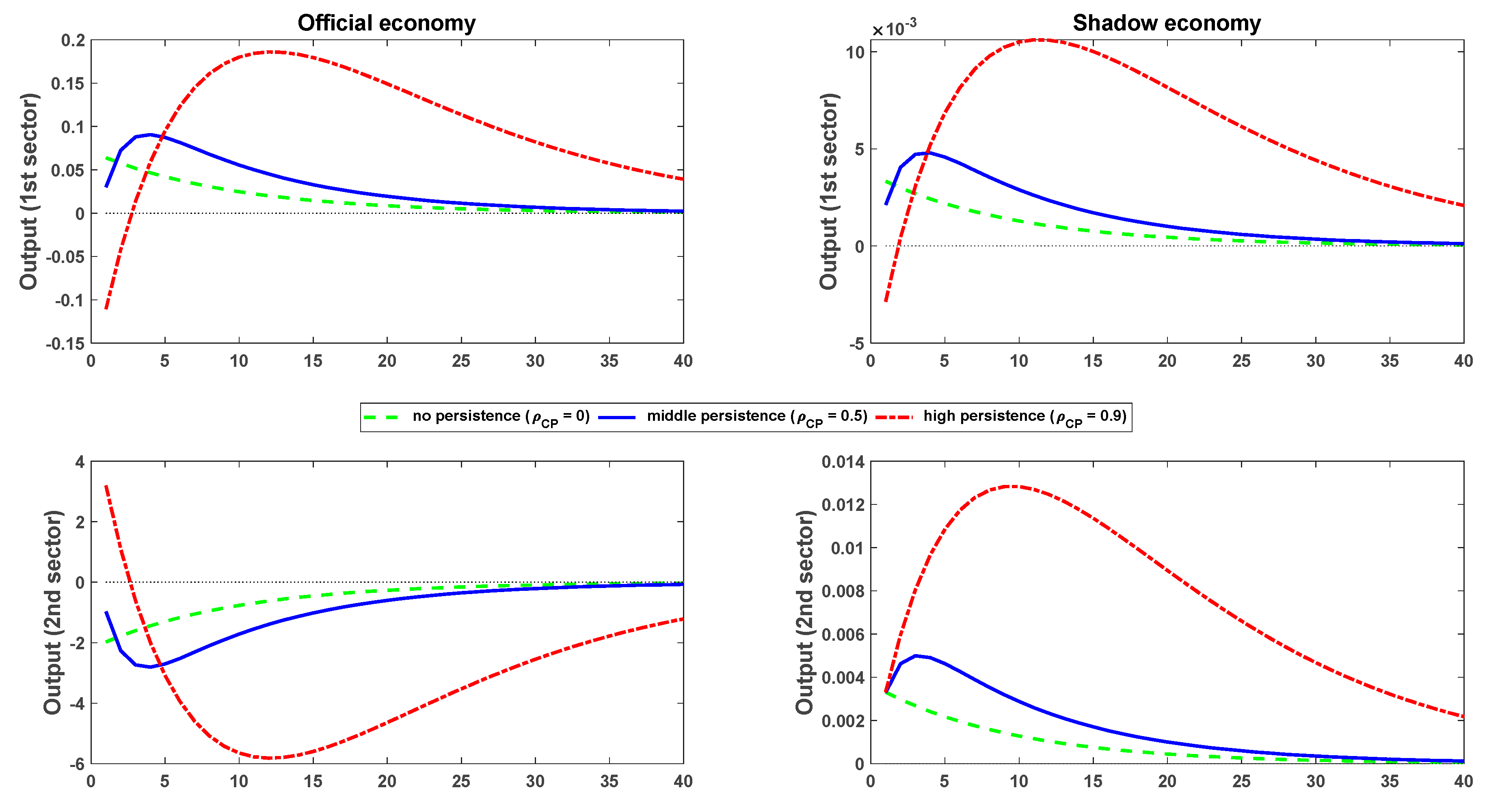
Figure 1 and Figure 2 graphically display the results of the simulations carried out. They describe the effects of shocks bearing the size of one standard deviation on the dynamics of capital, labour and output of individual sectors of the economy. Simulations were performed for alternative settings of shock persistence using the production perception indicator, , at 0 (no persistence), 0.5 (medium persistence) and 0.9 (high persistence). Zero persistence illustrates the relatively random and isolated corruption behaviour that is reflected in the perception of corruption deteriorating, which, however, quickly subsides and is not a systematic corruption phenomenon. On the contrary, the high persistence does not subside, as the given phenomenon means that the corrupt environment fundamentally deteriorates and across individual periods, it decreases by only 10% per period. It can in fact be identified with the corrupt environment’s systemic deterioration.
The figures show that in all cases, corruption moves the activities from the official economy to the shadow economy, which confirms the conclusions of the studies mentioned above. Regardless of whether it is a low persistence shock, manifested as a unique publicly presented corrupt behaviour, or whether it is a highly persistent act in the sense of creating an immanent corrupt environment. The transfer to the shadow economy occurs in the areas of labour, capital accumulation and actual production, that is, in case of both sources of economic growth as well as the growth of production itself. Activities are shifted to the shadow economy regardless of the specific modelled sector, that is, both in the sector burdened by excise taxes (fuel, alcohol, tobacco, etc.), which can be expected to have a significant tendency to tax evasion, and in the sector where no excise tax is imposed. The intensity of the activities transfer into the shadow economy zone is determined both by how persistent the perception of corruption is and by the type of production factor or sector of the economy.
The previous results clearly reveal that in all cases, the growth of corruption results in an increase in activity in the shadow economy sector, while the impact is greater the higher the persistence is (i.e., the expected persistence of the impulse in the perception of corruption). In simple terms, it is possible to confirm the intuitive opinion, which is also backed by theoretical studies and the empirical experience, that an increase in perceived corruption supports the shadow economy’s growth. However, an important finding emerging from the simulations is the fact that corruption and its perception have a significantly different effect on the two key production factors.
In the case of capital accumulation, gross fixed capital formation in the official economy shows a drop in all cases and referring to a situation of high persistence and the creation of a symptomatic corruption environment, this counts even four times than if it were a relatively rare corruption phenomenon. This is always accompanied by a mirrored increase in gross fixed capital formation within the shadow economy. It should be also mentioned that in case of high persistence, capital does not accumulate again in the official economy sector to its original level even after a shock subsides, neither does capital formation in the shadow economy return to its original level. Thus, we can state that if inertia in perceiving corruption persists, be it even without real corruption cases, the investment environment remains permanently distorted and the shadow economy is the preferred option for gross fixed capital formation. If a country shows a problematic corruption perception index, then this accounts for significant negative consequences in this area.
As for the second important long-term economic growth factor, the labour force size, in principle, it can be described via the processes in a similar way to capital accumulation. Taking a more detailed look at the results based on the above-mentioned figures, one fundamental fact cannot be overlooked. Although an indisputable shift of labour activities to the shadow economy occurs, these shifts are smaller by an order of magnitude, that is, about 10 times (measured in percent), lower than in the case of capital accumulation. Workforce changes in the official economy are also more complex. Especially the situation of the notoriously perceived corruption environment serves as an illustrative example (high persistence). Although a short-termed massive workforce size decline in the official economy occurs, comparable in percentage to the decline in capital accumulation, relatively soon, that is, after about four periods (one year) the original status and employment levels return. Afterwards, there are almost three years when the workforce in the official economy is increasing and then gradually declining, but this always refers to a value above the level prior to the simulating of the corruption induced shock. After a very long period of about 10 years, we may even find ourselves in a situation where the workforce size both in the official and the shadow economy figures is slightly above the level prior to the corruption-induced shock.
The above-mentioned is also illustrated in Figure 2, where the impacts on production are modelled. In a sector not burdened by an excise tax, that is, in the largest portion of our economy, there is a certain shift in activity to the shadow economy, but after a very short period, the official economy recovers and is better off than it would have been without a corruption shock. This even refers to the case of zero persistence and thus isolatedly occurring corruption. The graphical display of the official and shadow economy thus quite surprisingly reveals that objectively perceived corruption and an increase thereof stimulates production both in the official and the shadow economy, with the percentage increase in the official economy being higher by an order of magnitude.
The rationale for a shadow economy output growth can be relatively easily explained by the activities being transferred into this economy. The output growth in the official economy sector may represent a model mechanism, where losses due to increased corruption (associated with declining government revenues and the need to offset them via an implicit taxation increase within the official economy sector) make it necessary to increase production in order to provide for resources to meet tax obligations.
This article served to substantially widen the original Orsi model (2014) from the methodological point of view by adding the individual taxes of the usual tax mix. However, we did not restrain ourselves only to classifying taxes into direct and indirect ones as it is common in similar cases, but instead, we categorized individual partial tax items, too. This approach made it possible to identify another sector of the economy, representing taxes potentially prone to significant tax evasion. This production sector burdened by excise taxes is illustrated in the last part of Figure 2 and its impacts are entirely different. Undoubtedly, the production in the official economy shows a quite significant drop. It is evident that it is very difficult and time-consuming to reverse this practice and get back to the original state. The shadow economy growth in this sector is unquestionable as well. These data can be generalized in the sense that corruption has a significantly more destructive effect on that sector of the economy which is more prone to tax evasion. If such a sector has a relatively larger size in a given country, corruption also shows a more fatal effect on production generated in the official economy.
Unlike economic growth models, our model also allows us to examine and analyze a complete set of variables which describe the entire modelled economy in detail in the areas that are the subject of the article. With regard to the focus of the article, we can mention the characteristics of the modelled economy of the Czech Republic listed in Table 4. Our model including corruption and the real tax mix shows that net real wages in the official economy are almost 30% higher than in the shadow economy, and corruption can thus possibly affect the living standards of households. The size of the shadow economy makes 4.1%, which is a lower value than some other estimates based on not very sophisticated estimation methods using, for example, energy consumption or other indicators. These analyses are often not very robust and their conclusions are questionable.
Within the model presented by us, we believe that the size of the shadow economy is rather small, and is a kind of lower limit, which, however, is based on a complex structural model. In terms of sources of economic growth, the share of the workforce in the shadow economy is higher (4.9%) than the share of capital accumulation (3.2%), and it can be stated with a little simplification that corruption has a higher impact on labour in this sense.
6. Conclusions
This article and the results based on the estimates in it confirm many generalized ideas related to the link between corruption, economic growth and growth factors. Corruption and an increase in perceived corruption undoubtedly cause a shift of activities into the shadow economy sector. We can confirm this especially with respect to capital accumulation, where in particular a permanent corruption environment with a high persistence of corruption perception causes a permanent or at least very long-lasting reduced gross fixed capital formation in the official economy sector including its increased formation within the shadow economy. However, our results partially tear down the idea of corruption having an exclusively negative impact on the labour force size in the official economy sector while confirming the hypotheses about the rapid fading of this negative effect or even the positive effect. This may be both due to the concept of rational expectations as well as negotiations, and the above-mentioned motivation to compensate corruption-induced lost government spending. This is clearly reflected especially by the possible increasing size of production in the official economy in the case of goods which are not quite prone to tax evasion. A far as the sector with potential for tax evasion is concerned, that is, especially the fuel production sector, tobacco or alcohol, which are all subject to excise taxes, the growing corruption regarding production in the official economy sector has a clearly negative and even deadly impact.
The findings in the article confirm our assumption that the increase in perceived corruption supports the growth of the shadow economy, but also shows that corruption and especially its perception has a significantly different effect on two key pro-growth factors, capital accumulation and labour size. It further identifies another sector of the economy representing commodities burdened by taxes that are prone to tax evasion (excise taxes), and at the same time argues that corruption has a much more destructive effect on this sector of the economy. Under certain circumstances, these results may also be generalized for other post-communist EU Member States in a similar situation. We believe that these findings move knowledge in this area in a direction that has not yet been explored by more sophisticated methods.
As already mentioned, the use of DSGE modelling is currently a common way of describing economic reality. Unlike the (and often currently) theoretically used VAR models, which can often be perceived as an empirical exercise with a tendency to data mining, or also the usual panel regressions, DSGE models have an economic foundation based on economic theory. The behaviour of individual sectors of the economy, such as households, companies or the government, is precisely derived and modelled here. The model is thus in line with economic theory. The limit of DSGE modelling is the imposition of greater demands on the derivation or completion of the model itself in the theoretical level and the need for more sophisticated estimation techniques. At the same time, the limit of the model used may be its relative complexity. For example, Nobel laureate in Economics Milton Friedman (Friedman 1966) in his Methodology of Positive Economics recommends using those models that provide the best predictions and are also relatively simple, even regardless of the reality or unreality of the model’s assumptions. Another direction and a possible way of development of the presented topic is, at the empirical level, the estimation of the model using alternative indicators of corruption or taxation, or estimation on real data of other post-communist members of the European Union. However, the problem is obtaining some time series, especially concerning the penalty for tax evasion.
Author Contributions
Conceptualization, I.K. and D.N.; methodology, I.K., E.K., D.N. and Z.M.; validation, E.K. and Z.M.; formal analysis, D.N.; investigation, E.K. and Z.M.; resources, E.K. and Z.M.; data curation, D.N. and E.K.; writing—original draft preparation, I.K., D.N. and Z.M.; writing—review and editing, E.K. and Z.M.; project administration, I.K.; All authors have read and agreed to the published version of the manuscript.
Funding
This research was funded by the EACO, grant number EACO/RP08/2016, under the project “WTI Application in DSGE Modelling” and by the Technology Agency of the Czech Republic (TAČR), grant number TL02000210, under the project “Development of specialized software for measuring of tax burden and its application in the business sphere”.
Institutional Review Board Statement
Not applicable.
Informed Consent Statement
Not applicable.
Conflicts of Interest
The authors declare no conflict of interest.
References
- Adjemian, Stéphane, Houtan Bastani, Michel Juillard, Ferhat Mihoubi, George Perendia, Marco Ratto, and Sébastien Villemot. 2011. Dynare Reference Manual, Version 4. Dynare Working Papers for CEPREMAP, No. 1. Available online: https://EconPapers.repec.org/RePEc:cpm:dynare:001 (accessed on 20 November 2020).
- Auerbach, Alan J. 2017. Demystifying the Destination-Based Cash-Flow Tax. Brookings Papers on Economic Activity 2017: 409–432. [Google Scholar] [CrossRef] [Green Version]
- Baklouti, Nedra, and Younes Boujelbene. 2019. Shadow Economy, Corruption, and Economic Growth: An Empirical Analysis. The Review of Black Political Economy, 276–94. [Google Scholar] [CrossRef]
- Borlea, Sorin Nicolae, Monica Violeta Achim, and Monica Gabriela A. Miron. 2017. Corruption, Shadow Economy and Economic Growth: An Empirical Survey Across the European Union Countries. Available online: https://content.sciendo.com/configurable/contentpage/journals$002fsues$002f27$002f2$002farticle-p19.xml (accessed on 7 December 2020).
- Born, B., and J. Pfeifer. 2014. Policy Risk and the Business Cycle. Journal of Monetary Economics 68: 68–85. [Google Scholar] [CrossRef] [Green Version]
- Buehn, A., and F. Schneider. 2009. Corruption and the Shadow Economy: A Structural Equation Model Approach. IZA DP 4182. Available online: http://ftp.iza.org/dp4182.pdf (accessed on 12 December 2020).
- CNB. 2020. Czech National Bank: The ARAD Database. Available online: http://www.cnb.cz/docs/ARADY/HTML/index.htm (accessed on 12 December 2020).
- CZSO. 2020. National Accounts Statistics. Production and Pension Establishment Indicators. Available online: http://apl.czso.cz/pll/rocenka/rocenkavyber.socas (accessed on 8 December 2020).
- Donchev, D., and G. Ujhelyi. 2014. What Do Corruption Indices Measuere? Economic Politics 26: 309–31. [Google Scholar] [CrossRef]
- Dreher, A., and F. Schneider. 2010. Corruption and the Shadow Economy: An Empirical Analysis. Public Choice 144: 215–38. [Google Scholar] [CrossRef] [Green Version]
- Fjeldstam, O. H. 1996. Tax Evasion and Corruption in Local Governments in Tanzania: Alternative Economic Approaches. Available online: https://core.ac.uk/download/pdf/59168403.pdf (accessed on 12 December 2020).
- Fjeldstam, O. H. 2003. Fighting fiscal corruption: Lessons from the Tanzania Revenue Authority. Public Administration and Development 23: 165–175. [Google Scholar] [CrossRef]
- Frič, P. 2001. Corruption–Deviant Behaviour or Social Disorganisation? Sociologický Časopis (Czech Sociological Review) 37: 65–72. [Google Scholar] [CrossRef]
- Friedman, M. 1966. The Methodology of Positive Economics. In Essays In Positive Economics. Chicago: University of Chicago Press, vols. 30–43, pp. 3–16. [Google Scholar]
- Ghosh, S., and K. C. Neanidis. 2011. Corruption, Fiscal Policy, and Growth: A Unified Approach. London: Brunel University, pp. 1–42. [Google Scholar]
- Hoinaru, R., D. Buda, S. N. Borlea, V. L. Văidean, and M. V. Achim. 2020. The Impact of Corruption and Shadow Economy on the Economic and Sustainable Development. Do They “Sand the Wheels” or “Grease the Wheels?” Sustainability 12: 481. [Google Scholar] [CrossRef] [Green Version]
- Ivanyna, M., A. Moumouras, and P. Rangazas. 2010. The Culture of Corruption, Tax Evasion, and Optimal Tax Policy. Available online: https://mivanyna.files.wordpress.com/2018/02/ivanyna_mourmouras_rangazas_corruption_and_tax_policy_2010.pdf (accessed on 8 December 2020).
- Kaufmann, D. 2010. Can Corruption Adversely Affect Public Finances in Industrialized Countries? Available online: https://www.brookings.edu/opinions/can-corruption-adversely-affect-public-finances-in-industrialized-countries/ (accessed on 8 December 2020).
- Kirn, M., L. Umek, and I. Rakar. 2019. Transparency in Public Procurement–the Case of Slovenia. DANUBE Law Economics and Social Issues Review 10: 221–39. [Google Scholar]
- Kotlán, I., D. Němec, and Z. Machová. 2019. Legal Uncertainty in Taxation and Its Impacts on Labour Supply in the Czech Republic. Politická ekonomie (Political Economy) 67: 371–84. [Google Scholar] [CrossRef]
- Lindé, J. 2018. DSGE models: Still useful in policy analysis? Oxford Review of Economic Policy 34: 269–86. [Google Scholar] [CrossRef]
- Liu, Y., and H. Feng. 2014. Tax Structure and Corruption: Cross-Country Evidence. Public Choice 162: 57–78. [Google Scholar] [CrossRef] [Green Version]
- Medina, L., and F. Schneider. 2018. Shadow Economies Around the World: What Did We Learn over the Last 20 Years? IMF Working Paper, WP/18/17. Available online: https://www.imf.org/en/Publications/WP/Issues/2018/01/25/Shadow-Economies-Around-the-World-What-Did-We-Learn-Over-the-Last-20-Years-45583 (accessed on 8 December 2020).
- MFCR. 2020. Reports on the Financial Administration and the Customs Administration Activities in the 2002–2019 Period. Available online: http://www.mfcr.cz/cs/verejny-sektor/dane/danove-a-celni-statistiky/zpravy-o-cinnosti-financni-a-celni-sprav (accessed on 8 December 2020).
- Nye, J. S. 1967. Corruption and Political Development: A Cost-Benefit Analysis. American Political Science Review 61: 417–27. [Google Scholar] [CrossRef]
- Olken, B. A. 2009. Corruption Perception vs. Corruption Reality. Journal of Public Economics 93: 950–64. [Google Scholar] [CrossRef] [Green Version]
- Orsi, R., D. Raggi, and F. Turino. 2014. Size, Trend, and Policy Implications of the Underground Economy. Review of Economic Dynamics 17: 417–36. [Google Scholar] [CrossRef] [Green Version]
- Pappa, E., R. Sajedi, and E. Vella. 2015. Fiscal Consolidation with Tax Evasion and Corruption. Journal of International Economics 96: S56–S75. [Google Scholar] [CrossRef] [Green Version]
- PRS Group. 2020. International Country Risk Guide Methodology. Available online: https://www.prsgroup.com/explore-our-products/international-country-risk-guide/ (accessed on 7 December 2020).
- Shahab, M. R., J. Pajooyan, and F. Ghaffari. 2015. The Effect of Corruption on Shadow Economy: An Empirical Analysis Based on Panel Data. International Journal of Business and Development Studies 7: 85–100. [Google Scholar]
- Schneider, F. 2011. The Shadow Economy and Shadow Economy Labor Force: What Do We (Not) Know? IZA Discussion paper no. 5769, 1–66. Available online: https://www.iza.org/publications/dp/5769/the-shadow-economy-and-shadow-economy-labor-force-what-do-we-not-know (accessed on 7 December 2020).
- Solis-Garcia, M., and Y. Xie. 2018. Measuring the size of the shadow economy using a dynamic general equilibrium model with trends. Journal of Macroeconomics 56: 258–75. [Google Scholar] [CrossRef] [Green Version]
- Štork, Z., J. Závacká, and M. Vávra. 2009. DSGE Model of the Czech Republic. Ministry of Finance of the Czech Republic Working Paper 2/2009. Available online: https://www.mfcr.cz/cs/o-ministerstvu/odborne-studie-a-vyzkumy/2009/hubert-dsge-model-ceske-republiky-9444 (accessed on 7 December 2020).
- Torgler, B., and F. Schneider. 2009. The Impact of Tax Morale and Institutional Quality on the Shadow Economy. Journal of Economic Psychology 30: 228–45. [Google Scholar] [CrossRef] [Green Version]
- Transparency International. 2020a. Corruption Perceptions Index. Available online: https://www.transparency.org/en/cpi# (accessed on 6 December 2020).
- Transparency International. 2020b. Definition of Corruption. Available online: https://www.transparency.org/en/what-is-corruption (accessed on 7 December 2020).
- World Bank. 2020. World Bank Enterprise Survey. Available online: https://www.enterprisesurveys.org/ (accessed on 7 December 2020).
- Zubaľová, A., M. Geško, and M. Borza. 2020. Effectivity of Progressive Taxation from the Micro- and Macroeconomic Perspective. DANUBE Law Economics and Social Issues Review 11: 228–38. [Google Scholar]
Figure 1.
Shock impacts on the perception of corruption on the labour and capital markets.

Figure 2.
Shock impacts on the perception of corruption on an economy’s output.


Table 1.
Calibration of structural parameters.
| Parameter | Value | Description | Source: |
|---|---|---|---|
| 0.2 | share of dividend-paying companies | expert estimate | |
| 1 | inverse intertemporal substitution in consumption | logarithmic preferences | |
| 0.5 | inverse substitution elasticity among goods (both branches) | substitutability of goods from both sectors | |
| 0.05 | share of the second sector goods in total consumption | calibrated estimate based on production shares according to NACE categories | |
| 0.5 | inverse substitution elasticity of the consumption of goods from the shadow economy | substitutability of goods within the shadow economy (assumption similar to the official economy) | |
| 1.1 | coefficient of use from consumption, or work activities in the shadow economy | coefficient penalizing the consumption of shadow economy goods (scaling parameter) | |
| 0.99 | discount factor | Štork et al. (2009) | |
| 1.006 | economic potential growth rate | calibration based on data (average quarter-on-quarter GDP growth) | |
| 1 | coefficient of use from work activity | scaling parameter calibration | |
| 1 | Inverse elasticity of labour supply substitution | logarithmic preferences | |
| 5 | inverse elasticity of labour supply substitution in the shadow economy | the same value as for the official economy | |
| , | 1.2 | penalty coefficient for corporate income tax, VAT and excise duty | penalty estimate of 20% according to MFCR (2020) |
| 0.65 | Production labour factor share in sector 1 | calibration based on official economy data (same settings for shadow economy) | |
| 0.6 | Production labour factor share in sector 2 | ||
| 0.02 | capital depreciation rate | Orsi et al. (2014) | |
| 1.5 | the relative weight of perceiving the impact of corruption on corporate income tax | expert estimate based on analysing the tax elasticity effect | |
| 1.25 | the relative weight of perceiving the impact of corruption on personal income tax | expert estimate based on analysing the tax elasticity effect | |
| 1.25 | the relative weight of perceiving the impact of corruption on withholding tax | expert estimate based on analysing the tax elasticity effect | |
| 0.75 | the relative weight of perceiving the impact of corruption on social and health insurance contributions | expert estimate based on analysing the tax elasticity effect | |
| 1 | the relative weight of perceiving the impact of corruption on excise tax | expert estimate based on analysing the tax elasticity effect | |
| 1 | the relative weight of perceiving the impact of corruption on value-added tax | expert estimate based on analysing the tax elasticity effect |
Source: own calculations based on the DSGE model estimation.
Table 2.
Calibration of steady states of exogenous quantities.
| Variable | Value | Description | Comment |
|---|---|---|---|
| 1 | stable efficiency status of total investments | assumption of full average investment efficiency | |
| 1 | stable status in the use of work activities | calibrated value | |
| 1 | stable status in the price of goods in sector 1 of the official economy | Setting the numeraire (relative price) similar to Orsi et al. (2014) | |
| 1 | stable status of production technology in individual sectors of the economy | assuming the same efficiency in all sectors | |
| 0.028 | stable probability status of detection within sector 1 | data-based calibration | |
| 0.039 | steady probability status of detection within sector 2 | data-based calibration | |
| 0.15 | stable personal income tax rate | average rates for the 2002-2020 period | |
| 0.2285 | stable corporate income tax rate | ||
| 0.15 | stable withholding tax rate | ||
| 0.45 | stable social and health insurance contribution rates | ||
| 0.1444 | stable VAT rate | ||
| 3.47 | stable excise tax “rate” | expert estimate of the “average” rate for the 2002–2020 period |
Source: own calculations based on the DSGE model estimation. Note: the steady status calibration of endogenous quantities is based on the steady-state solution of the non-linear forms of the model.
Table 3.
Calibration of shock standard deviations.
| Shock | Standard Deviation | Comment |
|---|---|---|
| 0.0216 | calibration based on the estimated variability of tax revenue shocks | |
| 0.0390 | ||
| 0.0303 | ||
| 0.0116 | ||
| 0.0094 | ||
| 0.0150 | ||
| 0.0161 | calibration based on the observed values of the corruption perception indicator |
Source: own calculations based on the DSGE model estimation. Note: the setting of autoregressive shock parameters (except for the shock in the indicator of corruption perception) had an identical value of 0.9, similarly to the work of Orsi et al. (2014).
Table 4.
Selected additional characteristics of the modelled economy.
| Size of the shadow economy given by the shadow economy GDP-to-official economy GDP ratio | 4.1% |
| Shadow economy workforce-to-official economy workforce ratio | 4.9% |
| Shadow economy capital-to-official economy capital ratio | 3.2% |
| Shadow economy net real wages-to-official economy net real wages ratio | 129.2% |
Source: own calculations based on the DSGE model estimation. Note: The characteristics of the modelled economy are based on the calculation of the steady states of the nonlinear form of the DSGE model.
Publisher’s Note: MDPI stays neutral with regard to jurisdictional claims in published maps and institutional affiliations. |
© 2021 by the authors. Licensee MDPI, Basel, Switzerland. This article is an open access article distributed under the terms and conditions of the Creative Commons Attribution (CC BY) license (http://creativecommons.org/licenses/by/4.0/).
Share and Cite
MDPI and ACS Style
Němec, D.; Kotlánová, E.; Kotlán, I.; Machová, Z. Corruption, Taxation and the Impact on the Shadow Economy. Economies 2021, 9, 18. https://doi.org/10.3390/economies9010018
AMA Style
Němec D, Kotlánová E, Kotlán I, Machová Z. Corruption, Taxation and the Impact on the Shadow Economy. Economies. 2021; 9(1):18. https://doi.org/10.3390/economies9010018
Chicago/Turabian StyleNěmec, Daniel, Eva Kotlánová, Igor Kotlán, and Zuzana Machová. 2021. "Corruption, Taxation and the Impact on the Shadow Economy" Economies 9, no. 1: 18. https://doi.org/10.3390/economies9010018
Note that from the first issue of 2016, this journal uses article numbers instead of page numbers. See further details here.