Energy modeling of Hoeffding tree ensembles

1.Introduction

Energy consumption in machine learning is starting to gain importance in state-of-the-art research. This is clearly visible in areas where researchers are incorporating the inference or training of the model inside the device (i.e. edge computing or edge AI). An area whose main focus is on real-time prediction on the edge is data stream mining.

One of the most well-known and used classifier is the decision tree, due to its explainability advantage. In the data stream setting, where we can only do one pass over the data, and we can not store all of it, the main problem of building a decision tree is the need to reuse the examples to compute the best splitting attributes. Hulten and Domingos [16] proposed the Hoeffding Tree or VFDT, a very fast decision tree for streaming data, where instead of reusing instances, we wait for new instances to arrive. The most interesting feature of the Hoeffding tree is that it builds an identical tree with a traditional one, with high probability if the number of instances is large enough, and that it has theoretical guarantees about that.

Decision trees are usually not used alone, but within ensembles methods. Ensemble methods are combinations of several models whose individual predictions are combined in some manner (e.g., averaging or voting) to form a final prediction. They have several advantages over single classifier methods: they are easy to scale and parallelize, they can adapt to change quickly by pruning under-performing parts of the ensemble, and they therefore usually also generate more accurate concept descriptions.

Advancements in data stream mining have been primarily focused on creating algorithms that output higher predictive performance. For that, they used ensembles of existing algorithms. However, these solutions output high predictive performance at the cost of higher energy consumption. We recently conducted an experiment comparing Online Boosting [34, 35] to standard Hoeffding trees for the Forest dataset (Section 5.1). Online Boosting was able to achieve 14% more accuracy but consuming 5 times more energy. To address this challenge, we present the nmin adaptation method for ensembles of Hoeffding Tree algorithms [16], to make them more feasible to run in the edge.

The nmin adaptation method is a method presented in [18], which reduces the energy consumption of standard Hoeffding tree algorithms by adapting the number of instances needed to create a split. We extend that study by incorporating the nmin adaptation method to ensembles of Hoeffding trees. The goal of this paper is two-fold:

We have conducted experiments on five different ensembles of Hoeffding trees (Leveraging Bagging [6], Online Coordinate Boosting [37], Online Accuracy Updated Ensemble [11], Online Bagging [36],and Online Boosting [36]), with and without nmin adaptation, on 11 publicly available datasets. The results show that we are able to reduce the energy consumption by 21%, affecting accuracy by less than 1%, on average.

This approach achieves similar levels of accuracy as state-of-the-art ensemble online algorithms, while significantly reducing its energy consumption. We believe this is a significant step towards a greener data stream mining, by proposing not only more energy efficient algorithms, but also creating a better understanding of how ensemble online algorithms consume energy.

The rest of the paper is organized as follows: The work related to this study is presented in Section 2. Background on Hoeffding trees and the nmin adaptation method is presented in Section 3. The main contribution of this paper is presented in Section 4. There we first describe how to build energy models for any kind of algorithm (Fig. 2), we then present extensive theoretical energy models for the Online Bagging, Leveraging Bagging, Online Boosting, Online Coordinate Boosting, and Online Accuracy Updated Ensemble algorithms. This helps at understanding the energy bottlenecks of the algorithm, and why nmin adaptation is efficient at handling those bottlenecks. The design of the experiments together with the results are presented in Sections 5 and 6 respectively. The paper ends with conclusions in Section 7.

2.Related work

Energy efficiency has been widely studied in the field of computer architecture for decades [23]. Moore’s law stated that the performance of CPUs was going to double every 18 months, by doubling the number of transistors. This prediction was made considering one fundamental constraint, that the energy consumed by each unit of computing would decrease as the number of transistors increased.11 The CPU scaling from Moore does not apply anymore, and the main reason is because there was not enough focus on scaling the power while increasing performance [25]. This has created a paradigm shift, where power is the key factor studied to improve computer performance, creating processors that handle more operations using the same amount of power [28].

Machine learning research, and in particular deep learning, is aware of the need to focus not only on creating more accurate models, but also on creating energy efficient models [21, 20, 38]. The researchers in this area have realized that the amount of energy and resources (e.g. GPUs) needed to perform training and inference on such models is impractical, especially for mobile platforms. Currently most of the machine learning models used in the phone are accessed through the cloud, since doing inference in the phone is challenging. Some research is going in that direction, such as The Low Power Image Recognition Challenge (LPIRC) [19], and the work by [13, 39].

Approaches to mine streams of data have been evolving during the past years. We consider the Hoeffding tree algorithm [16] to be the first algorithm that was able to classify data from an infinite stream of data in constant time per example. That approach was later improved to be able to handle concept drift [26], that is, non-stationary streams of data that evolve through time. The ability to handle concept drift introduces many computational demands, since the algorithm needs to keep track of the error to detect when a change occurs. ADWIN (adaptive windowing) [3] is the most efficient change detector that can be incorporated to any algorithm. The Hoeffding Adaptive Tree (HAT) [4] was introduced as an extension to the standard Hoeffding tree algorithm that is able to handle concept drift using the ADWIN detector.

In relation to energy efficiency and data stream mining, several studies have recently focused on creating more energy efficient versions of existing models. The Vertical Hoeffding Tree (VHT) [29] was introduced to parallelize the induction of Hoeffding trees. Another approach for distributed systems is the Streaming Parallel Decision Tree algorithm (SPDT) [2]. Marrón et al. [33] propose a hardware approach to improve Hoeffding trees, by parallelizing the execution of random forests of Hoeffding trees and creating specific hardware configurations. Another streaming algorithm that was improved in terms of energy efficiency was the KNN version with self-adjusting memory [30].

A recent publication at the International Conference on Data Mining [31] presented an approach similar to ours, which estimates the value of nmin to avoid unnecessary split attempts. Although their approach seems to better estimate the value of nmin, our approach is still more energy efficient (based on their results), which is the ultimate goal of our study. We believe that trading off a few percentages of accuracy is necessary in some scenarios (e.g. embedded devices) where energy and battery consumption is the main concern. This work is an extension of an already published study where we introduced nmin adaptation [18]. While in that work the nmin adaptation method was only applied to the standard version of the Hoeffding tree algorithm, this study proposes more energy efficient approaches to create ensembles of Hoeffding trees, validated by the experiments on five different algorithms and 11 different datasets. On top of that, this study presents, to the best of our knowledge, the first approach to create generic energy model for any class of machine learning algorithm.

3.Background

This section explains in detail Hoeffding trees, together with the ensembles of Hoeffding trees used in this study.

3.2nmin adaptation

The nmin adaptation method was previously introduced in [18]. While that study only focused on the energy reduction of standard Hoeffding tree algorithms, this study proposes to use the nmin adaptation method on ensembles of Hoeffding trees, to align with the current approaches in data stream mining.

The goal of the nmin adaptation method is to estimate the number of instances (nmin) that are needed to make a split with confidence 1-δ. Current Hoeffding tree algorithms use a fixed value of nmin instances. Thus the batch of instances that are observed on each node before checking for a possible split is the same for each node, and during the complete execution of the algorithm. As is explained in Section 4.2.1, having a fixed nmin value is energy inefficient. This is because there are many times where those instances are not enough to make a confident split, thus all those computations are done unnecessarily.

Our method estimates, for each node, the nmin instances that ensure a split, to calculate the splitting attributes only when there is going to be a split. Since each node will have their own nmin, we allow the tree to grow faster (lower nmin) in those branches where there is a clear attribute to split on, and to delay the growth (higher nmin) in those branches where there is no clear attribute to split on.

Figure 1.

Example of the nmin adaptation method. The value of nmin is going to be adapted based on two scenarios: scenario 1 (left plot), and scenario 2 (right plot).

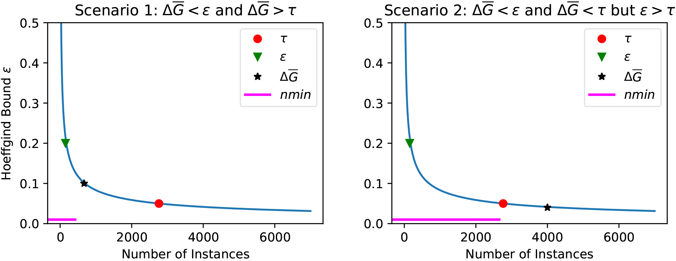
The value of nmin is going to be adapted only when a non-split occurs, otherwise we assume that the current value is the optimal one. The method follows two approaches, illustrated in Fig. 1.

The first approach (scenario 1) approximates the value of nmin when the non-split occurred because no attribute was the clear winner (Fig. 1 left plot). In this case, nmin is estimated as the number of instances needed for the best attribute to be higher than the second best attribute with a difference of ε. Taking a look at the left plot from Fig. 1, nmin are the instances needed for the green triangle (ε), to reach the black star(Δ⁢G¯). When we wait for those nmin instances, then Δ⁢G¯>ε, satisfying the condition for a split. More formally, for the first scenario:

(2)

𝑛𝑚𝑖𝑛=⌈R2⋅ln⁡(1/δ)2⋅(Δ⁢G)2⌉

The second approach (scenario 2) approximates the value of nmin when the non-split occurred because ε>τ. In this scenario, although the attributes are very similar (Δ⁢G¯<ε), and their difference in entropy is smaller than τ, the confidence is still not high enough to make a split. Taking a look at the right plot from Fig. 1, nmin are the instances needed for the green triangle (ε), to reach the red dot (τ). When we wait for those instances, then ε<τ, satisfying the condition to create a split. More formally, the nmin approximation for the scenario 2 is defined as:

(3)

𝑛𝑚𝑖𝑛=⌈R2⋅l⁢n⁢(1/δ)2⋅τ2⌉

The nmin adaptation implemented for the Hoeffding tree algorithm is portrayed in Algorithm 1.

[tbh] Hoeffding Tree with nmin adaptation. Symbols:nmin: hyperparameter initially set by the user that is going to be adapted; H⁢T: Initial tree; X: set of attributes; G⁢(⋅): split evaluation function; τ: hyperparameter used for attributes with tied information gain[1] stream is not empty Read instance Traverse the tree using H⁢TUntil leaf l is reached Update statistics at leaf lNominal and numerical attributes Increment nl: instances seen at lnmin⩽nlAttemptSplit(l) Call Function from Algorithm 3.1Split==True CreateChildren(l) New leaf lm with initialized statistics Disable attr {Xp⁢|(G¯l⁢(Xp)-G¯l⁢(Xa))>⁢ε}Adapt the value of nmin Δ⁢G¯⩽τ𝑛𝑚𝑖𝑛=⌈R2⋅l⁢n⁢(1/δ)2⋅τ2⌉Scenario 2 𝑛𝑚𝑖𝑛=⌈R2⋅l⁢n⁢(1/δ)2⋅(Δ⁢G)2⌉Scenario 1

4.Energy modeling of Hoeffding tree ensembles

This section presents the main contribution of this paper, guidelines on how to construct energy efficient ensembles of Hoeffding trees, validated with the experiments on Section 6. In order to reduce the energy consumption of ensembles of Hoeffding trees, we apply the nmin adaptation method to the Hoeffding tree algorithm, and use that algorithm as the base for the different ensembles. To have a more detailed view on how energy is consumed on ensembles of Hoeffding tees, we first portray an approach to create generic theoretical energy models for any kind of algorithm (Section 4.1). We then show how that generic approach applied for ensemble of Hoeffding trees (Section 4.2 and Fig. 3). That section finalizes with a detailed energy model and explanation of each algorithm: Online Bagging, Online Boosting, Leveraging Bagging, Online Coordinate Boosting, Online Accuracy Updated Ensemble, and Hoeffding tree with nmin adaptation.

4.1Generic approach to create energy models

We have summarized the different steps to create theoretical energy models in Fig. 2.

Figure 2.

Generic approach to build energy models for any kind of algorithm.

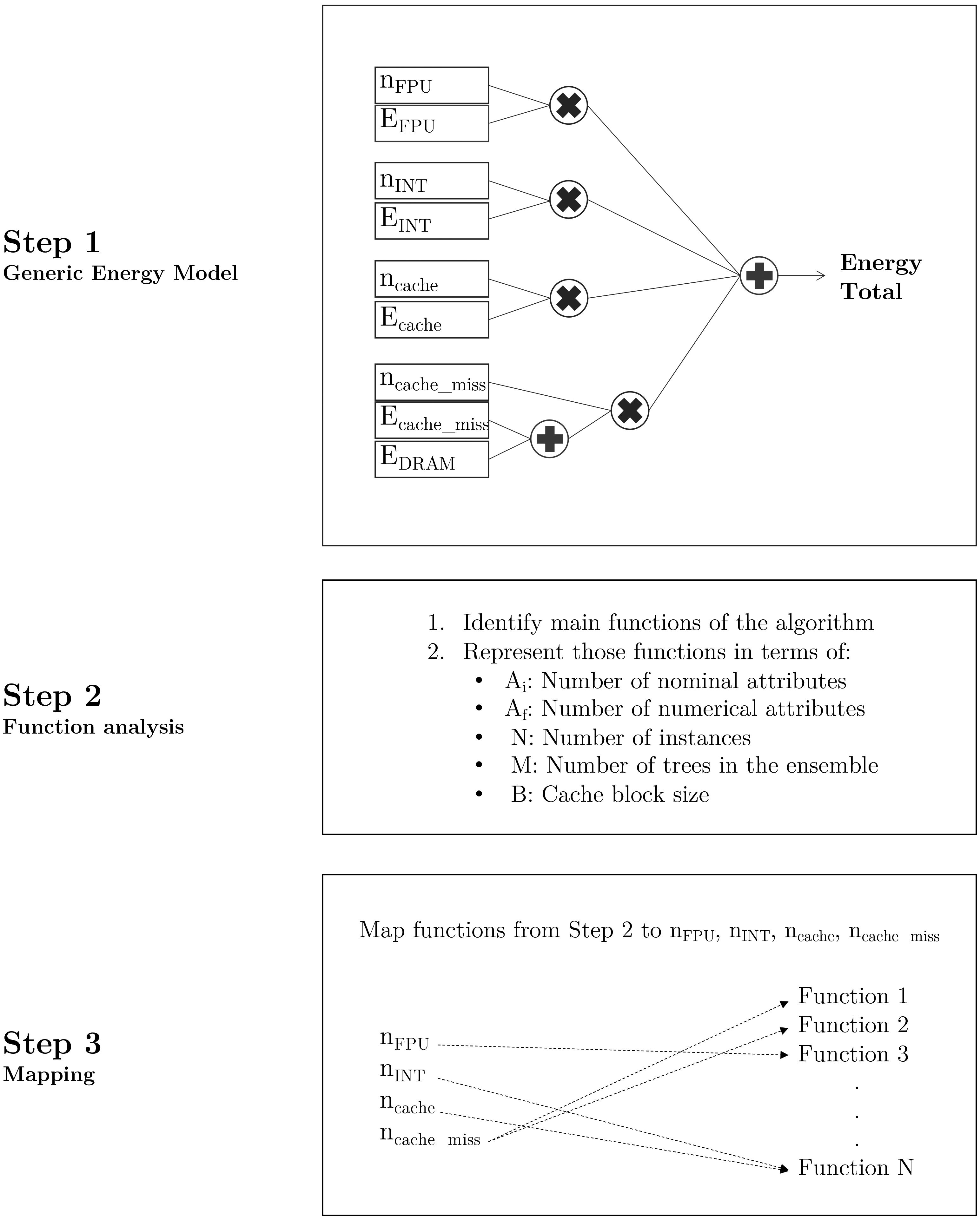
First, Step 1 formalizes the generic energy model, as a sum of the different operations (mapped then to algorithm functions) categorized by type of operation. Thus, the total energy of a model can be expressed as:

E=n𝐹𝑃𝑈⋅E𝐹𝑃𝑈+n𝐼𝑁𝑇⋅E𝐼𝑁𝑇+n𝑐𝑎𝑐ℎ𝑒⋅E𝑐𝑎𝑐ℎ𝑒+ncache_miss⋅(Ecache_miss+E𝐷𝑅𝐴𝑀)

The operations are divided into integer, floating point operations, and DRAM and cache accesses. We consider a DRAM access everytime a cache miss occurs. The energy per access or per computation (E𝐹𝑃𝑈,E𝐼𝑁𝑇,Ecache_miss,E𝐷𝑅𝐴𝑀) will depend on the specific hardware where the algorithm is run. However, knowing which type of operations consumes more energy (example a DRAM access consumes 100 times more energy than a floating point operation), together with the amount of operations for each type, gives a detailed overview of the theoretical energy consumption of the algorithm. Step 1 can be done only once, as appears in the figure, and can be used for any algorithm. It can be adapted to specific hardware components if needed.

Step 2 focuses on identifying the main functions of the algorithm, and then representing them in terms of generic features such as number of attributes or size of the ensemble.

In Step 3 the goal is to map the functions from Step 2 to the different type of operations. For example, a function that counts the number of instances can be expressed as one integer operation per instance.

An example of how to apply these steps is shown in Section 4.2.

4.2Ensembles energy models

The process to create an energy model for any ensemble of other algorithms is summarized in Fig. 3. The goal is to combine the energy model of the ensemble and the energy model of the base algorithm for the ensemble. In the case of Online Bagging, for instance, we need to sum the energy model of Online Bagging plus the energy model of the Hoeffding tree with nmin adaptation. If another model is used in the ensemble, it can be substituted by the Hoeffding tree with nmin adaptation (dashed box).

Figure 3.

Energy model approach for ensembles of Hoeffding trees with nmin adaptation. Steps: i) Obtain the energy model (following Fig. 2) for the general ensemble of trees; ii) Obtain the energy model of Hoeffding trees with nmin adaptation; iii) Sum the energy model variables. The energy model for Hoeffding trees (dashed box) can be substituted by the energy model of any other algorithm that is going to be part of the ensembles (for example Hoeffding Adaptive Trees [4]).

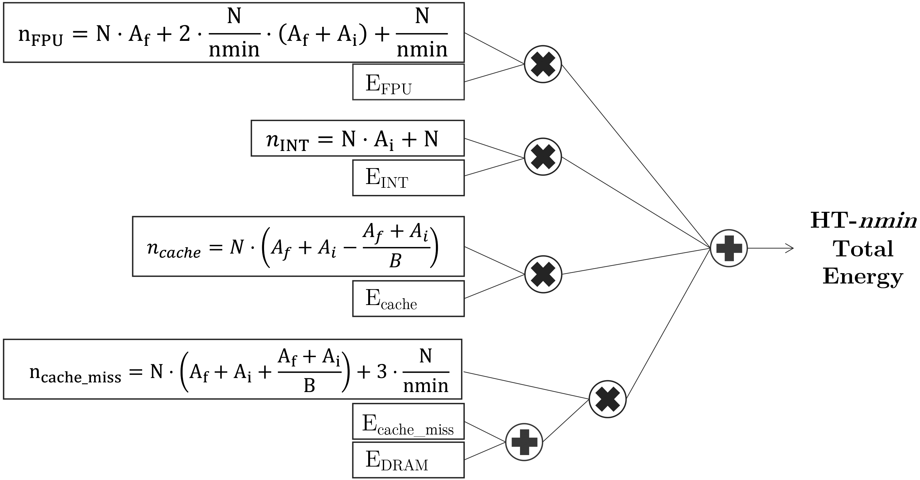
Figure 4.

Energy model for the Hoeffding tree with nmin adaptation.

This section details, first, the energy model of Hoeffding Trees with nmin adaptation (Fig. 4), then the energy models of the ensembles: Online Bagging (Fig. 5), Leveraging Bagging (Fig. 6), Online Boosting (Fig. 7), Online Coordinate Boosting (Fig. 8), Online Accuracy Updated Ensemble (Fig. 9).

4.2.1Hoeffding trees with nmin adaptation

The energy consumption of Hoeffding trees with nmin adaptation (HT-nmin for the remainder of the paper), explained in detail in Section 3.2, is summarized with the energy model from Fig. 4.

The second step (Fig. 2) after defining the generic energy model is to identify the main functions of the HT-nmin. The HT-nmin algorithm spends energy on training (traversing the tree, updating the statistics, checking for a split, doing a split), and doing inference (traversing the tree, Naive Bayes or majority class prediction at the leaf). In particular:

• • Traverse the tree: The energy spent on traversing the tree is calculated as the number of cache misses, which we assume as one access per attribute per instance (for every time as instance is read), as the worst case scenario.

• • Updating statistics: The energy spent on updating statistics is divided in nominal and numerical attributes. The energy spent in updating attributes regarding computations is one integer computation per instance per nominal attribute, and one floating point operation per numerical attribute. In terms of accesses, for both nominal and numeric attributes, we have a cache miss the first time we access the table, and then one cache hit per nominal attribute, and then a cache miss for every attribute that exceeds the block size.

• • Checking for a split: To check for a split we need to calculate the entropy for all attributes, calculate the Hoeffding bound, and sort the attributes to obtain the best one. Calculating the entropy, calculating the Hoeffding bound, and sorting the attributes, is one floating point operation per attribute, every nmin instances. Regarding memory accesses, we consider one cache miss every nmin instances.

• • Doing a split: To create a new node we consider one floating point operation and one cache miss every nmin instances.

Finally, those functions are mapped to the corresponding n𝐹𝑃𝑈,n𝐼𝑁𝑇,n𝑐𝑎𝑐ℎ𝑒,ncache_miss, as shown in Fig. 4.

What we believe is more important to observe from this energy model is the impact of the nmin parameter. The amount of times that the algorithm check for split, which involves a significant part of the energy consumption, depends on the value of nmin. That is why having a bad approximation of nmin incurs in high energy costs without increasing the predictive performance. This model is the input presented in the energy models of the ensembles from the following paragraphs.

4.2.2Online Bagging

Online Bagging, presented in Algorithm 4.2.2, was proposed by Oza and Russell [36] as a streaming version of traditional ensemble bagging. Bagging is one of the simplest ensemble methods to implement. Non-streaming bagging [9] builds a set of M base models, training each model with a bootstrap sample of size N created by drawing random samples with replacement from the original training set. Each base model’s training set contains each of the original training examples K times where P(K=k) follows a binomial distribution:

P(K=k)=(nk)pk(1-p)n-k=(nk)1nk(1-1n)n-k.

This binomial distribution for large values of n tends to a Poisson(1) distribution, where Poisson(1) =exp⁡(-1)/k!. Using this fact, [36] proposed Online Bagging, an online method that instead of sampling with replacement, gives each example a weight according to Poisson(1).

[htb] Online Bagging(h,d)[1] each instance deach model hm,(m∈1,2,…,M)k=𝑃𝑜𝑖𝑠𝑠𝑜𝑛(λ=1)Train the model on the new instance k times

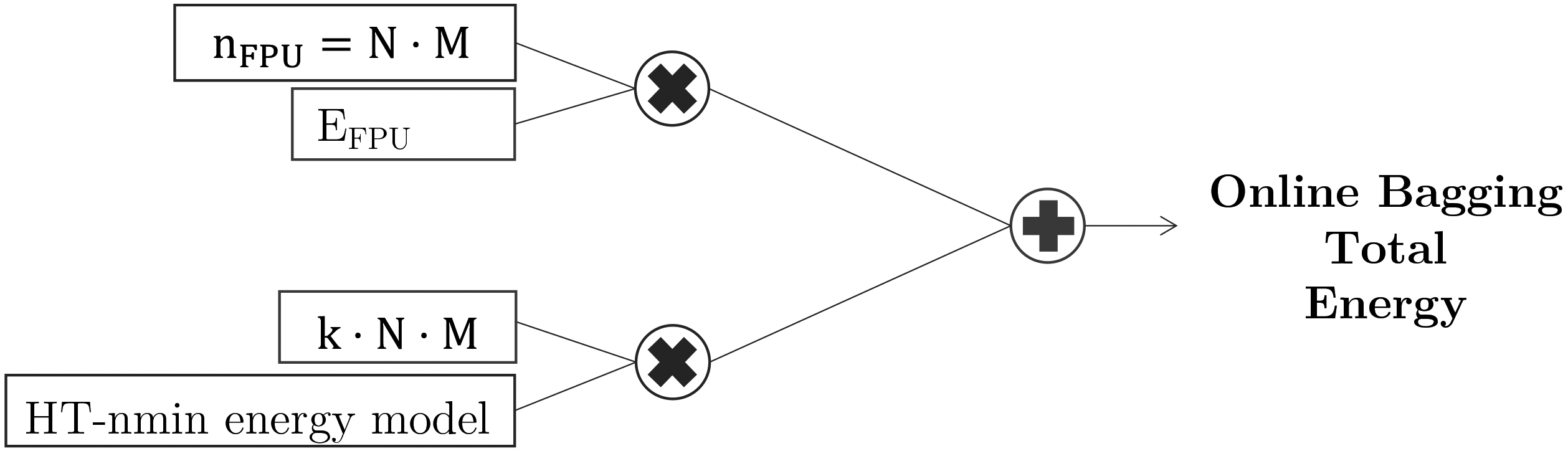
This algorithm has two main functions, one involved in training the model, that depends on the base algorithm, and the other function that calculates k. Training the model can be represented as the energy model of the Hoeffding tree with nmin adaptation, from Fig. 4. Calculating k involves one floating point operation per instance (N) per model (M). The final energy model for Online Bagging is represented in Fig. 5.

4.2.3Leveraging Bagging

When data is evolving over time, it is important that models adapt to the changes in the stream and evolve over time. ADWIN bagging [7] is the online bagging method of Oza and Russell with the addition of the ADWIN algorithm [3] as a change detector and as an estimator for the weights of the boosting method. When a change is detected, the worst classifier of the ensemble of classifiers is removed and a new classifier is added to the ensemble. Leveraging Bagging [6], shown in Algorithm 5, extends ADWIN bagging by leveraging the performance of bagging with two randomization improvements: increasing resampling and using output detection codes. Leveraging bagging increases the weights of this resampling using a larger value λ to compute the value of the Poisson distribution. For every instance, on top of training the model for each ensemble as for Online Bagging, Leveraging Bagging checks if the instance is correctly classified by the model, and inputs such error value to the ADWIN detector (Algorithm 5), to check for a possible change.

Figure 5.

Online Bagging energy model based on the number of models (M) and number of instances (N), considering the Hoeffding tree with nmin adaptation as the base tree classifier.

[ht] ADWIN. Symbols:h: ensemble of models hm: model in particular. d: instance[1] y𝑝𝑟𝑒𝑑= Classify instance d with classifier hmy= True class of dy𝑝𝑟𝑒𝑑 == ycorrectlyClassifies ← True 𝐸𝑟𝑟𝐸𝑠𝑡𝑖𝑚= getEstimation(hm) setInput(hm, correctlyClassifies) == True getEstimation(hm) >E⁢r⁢r⁢E⁢s⁢t⁢i⁢mAfter new input from Line 8 Change ← True [ht] Leveraging Bagging(h,d,λ)[1] each instance deach model hm,(m∈1,2,…,M)k=𝑃𝑜𝑖𝑠𝑠𝑜𝑛⁢(λd)Train the model on the new instance k times ADWIN(h,hm,d) Call function from Algorithm 5ADWIN detects change on hmReplace classifier with highest error with a new classifier

Figure 6.

Energy model for Leveraging Bagging. N= number of instances, M= number of models, W= window size, s= speed of change, c= percentage of correctly classified instances.

Leveraging Bagging has a similar energy consumption pattern than Online Bagging with the addition of the ADWIN detector and the output codes. The ADWIN detector introduces significant overhead since it has to keep track of the error. For every instance ADWIN calculates if model hm correctly classifies instance d, for each model hm,(m∈1,2,…,M). It then inputs a 0 for misclassification or 1 for a correct classification to the ADWIN detector. With this information, ADWIN outputs if there has been a change in the current window. If the size of the window exceeds the maximum value assigned, ADWIN resizes the window. Finally, if a change is detected, the worst performing classifier is removed from the ensemble, and a new one is created.

The main functions of the baseline algorithm are: calculate k, train with HT-nmin, and replace classifier. The main functions of ADWIN are: traverse the tree, obtain the true class y, compare y with the prediction, get the estimation, and set the input to ADWIN. The following list details these functions in terms of type of operations and number of instances, models, etc. Computing the output codes are omitted since they are not activated by default in the algorithm.

• • Calculate k is one FPU operation per instance per model.

• • Replacing the classifier is one cache miss per classifier to get the error of each classifier, and one cache miss to replace it. That is per instance per model per everytime change is detected (S variable).

• • Traverse the tree. As for the HT-nmin, the energy is calculated as the number of cache misses, assuming one access per attribute per instance.

• • Obtaining the true class is one cache miss per instance per model.

• • Comparing y with the prediction is one cache access per instance per model.

• • Getting the estimation is just dividing the amount of error by the number of instances, which outputs to one floating point operation per instance per model.

• • Setting the input is quite energy consuming, since there are several operations involved. First it inserts the element in the window bucket, which is one cache miss per instance per model. Second it compresses the buckets, which we calculate as one cache miss per instance per model for the first access, and then (log(W)-1) cache accesses per instance per model for the rest of the window accesses, W being the window size. Third it reduces the window, which is the same energy consumption pattern as compressing the buckets, one cache miss per instance per model and (log(W)-1) cache accesses per instance per model.

Figure 6 shows the energy model of the Leveraging Bagging algorithm, based on the function explanations presented in the previous list. M is the number of models in the example, N the number of instances, W is the window size for ADWIN, s is the speed of change (the percentage of instances with change), c is the percentage of correctly classified instances.

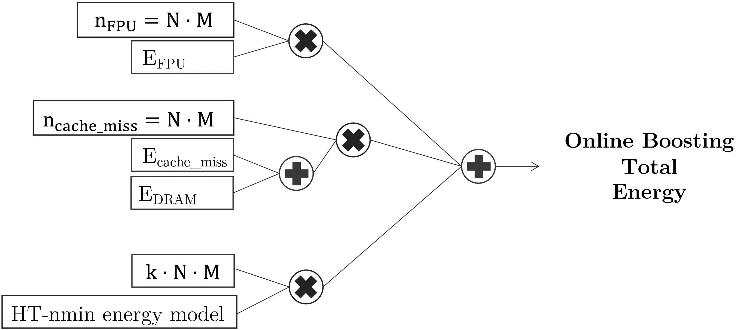
4.2.4Online Boosting

Online Boosting [34, 35] is an extension of boosting for streaming data, presented in Algorithm 4.2.4. The main difference with Online Bagging is that Online Boosting updates the λ of the Poisson distribution for the next classifier based on the preformance of the current classifier (Fig. 4). If classifier m classifies the instance correctly, that instance will be assigned a lower weight for the next classifier m+1. On the other hand, if the instance is classified incorrectly, that instance gets updated with a higher weight. Each instance is passed through each model in sequence.

[ht] Online Boosting(h,d)[1] λd=1each instance deach model hm,(m∈1,2,…,M)k=𝑃𝑜𝑖𝑠𝑠𝑜𝑛⁢(λd)Train the model on the new instance k times instance is correctly classified instance weight λd updated to a lower value instance weight λd updated to a higher value

Regarding its energy consumption and energy model, we observe that Online Boosting presents a similar energy consumption pattern than Online Bagging. Online Bagging introduces an extra memory access to update the weight, which we assume that the access is a DRAM access because each instance is updated sequentially, not fitting in cache. We assume one instance update per instance per model, the worst case scenario if all instances are classified incorrectly. The detailed energy model is presented in Fig. 7.

Figure 7.

Online Boosting energy model based on the number of models (M) and number of instances (N), considering the Hoeffding tree with nmin adaptation as the base tree classifier. k represents the output value of the Poisson distribution from Algorithm 4.2.4, line 4.

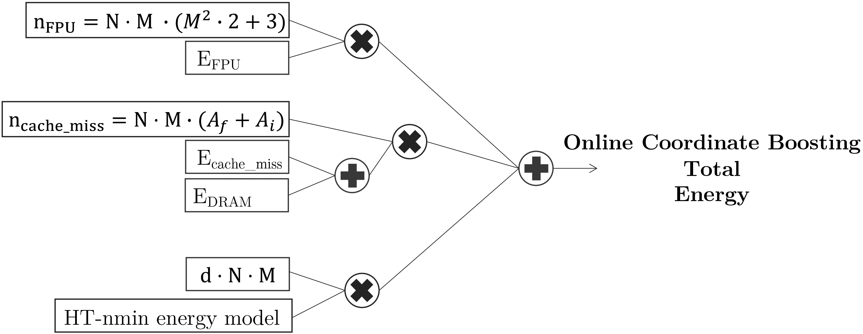
4.2.5Online Coordinate Boosting

Online Coordinate Boosting [37](Algorithm 4.2.5) is an extension to Online Boosting, that uses a different procedure to update the weight, to yield a closer approximation to Freund and Schapire’s AdaBoost algorithm [17]. The weight update procedure is derived by minimizing AdaBoost’s loss when viewed in an incremental form.

From Algorithm 4.2.5 we can observe the different calculations in lines 8, 11, 13, 14, and 15. Once the weight is calculated, the HT-nmin algorithm is trained with weight d. They use the following formulas to calculate πj+, πj+, Wj⁢k+ and Wj⁢k-.

[h] Online Coordinate Boosting(h,x)[1] d=1each instance xeach model hm,(m∈1,2,…,M)instance is correctly classified mj=1every model seen so far -1 Calculate πj+ and πj+ using Eqs (4) and (5) every model seen so far Calculate Wj⁢k+ and Wj⁢k- using Eqs (6) and (7) αji=12⁢log⁡Wj⁢j+Wj⁢j-Δ⁢αj=αji-αji-1d←d⁢e-αji⁢mi⁢jTrain the model on the new instance with weight d

(4)

πj+=∏k=j0j-1(Wj⁢k+Wj⁢j+⁢e-Δ⁢αk+(1-Wj⁢k+Wj⁢j+)⁢eΔ⁢αk)

(5)

πj-=∏k=j0j-1(Wj⁢k-Wj⁢j-⁢e-Δ⁢αk+(1-Wj⁢k-Wj⁢j-)⁢eΔ⁢αk)

(6)

Wj⁢k+=Wj⁢k+⁢πj++d⁢𝟏[mi⁢k=+1]⋅𝟏[mi⁢j=+1]

(7)

Wj⁢k-=Wj⁢k-⁢πj-+d⁢𝟏[mi⁢k=-1]⋅𝟏[mi⁢j=-1]

where j represents the model of the ensemble, j0 is set to 0, and mj is defined in line 5 of the algorithm. To iterate over the product we introduced the loops in lines 7 and 10.

In relation to energy consumption, this energy model, presented in Fig. 8 adds the extra floating point operations of calculating the values of Wj⁢k, πj, αji, Δ⁢αj, and d, and the cache accesses related to traversing the tree to calculate if the instance is correctly classified. Traversing the tree is the same as for ADWIN, one access per attribute per instance. Calculating πj can be estimated as

∑k=0M-1k,

and Wj⁢k as

∑k=0Mk.

Since the sum of πj and Wj⁢k result in M2 operations, the amount of floating point operations of lines 8 and 11 can be simplified as: M⋅N⁢(M2⋅2+3). Finally, lines 13, 14, and 15 of Algorithm 4.2.5 require one floating point operation per instance per model.

Figure 8.

Energy model for Online Coordinate Boosting.

4.2.6Online Accuracy Updated Ensemble

Batch-incremental methods create models from batches, and they remove them as memory fills up; they cannot learn instance-by-instance. The size of the batch must be chosen to provide a balance between best model accuracy (large batches) and best response to new instances (smaller batches). The Online Accuracy Updated Ensemble (OAUE) [11, 12], presented in Algorithm 4.2.6 maintains a weighted set of component classifiers and predicts the class of incoming examples by aggregating the predictions of components using a weighted voting rule. After processing a new example, each component classifier is weighted according to its accuracy and incrementally trained.

[ht] Online Accuracy Updated Ensemble. Symbols:ε: ensemble w: window M: ensemble size [1] ε←∅C′←new candidate classifier each instance xtCalculate the prediction error of all classifiers Ci∈ε on xtt>0andt mod w = 0 |ε|<MAdd classifier C′ to the ensemble εweight all classifiers Ci∈ε and C′ using Eq. (8) substitute least accurate classifier in ε with C′C′← new candidate classifier incrementally train classifier C′ with xtweight all classifiers Ci∈ε using Eq. (8)

all classifiers Ci∈εincrementally train classifier Ci with xt

Figure 9.

Energy model for Online Accuracy Updated Ensemble.

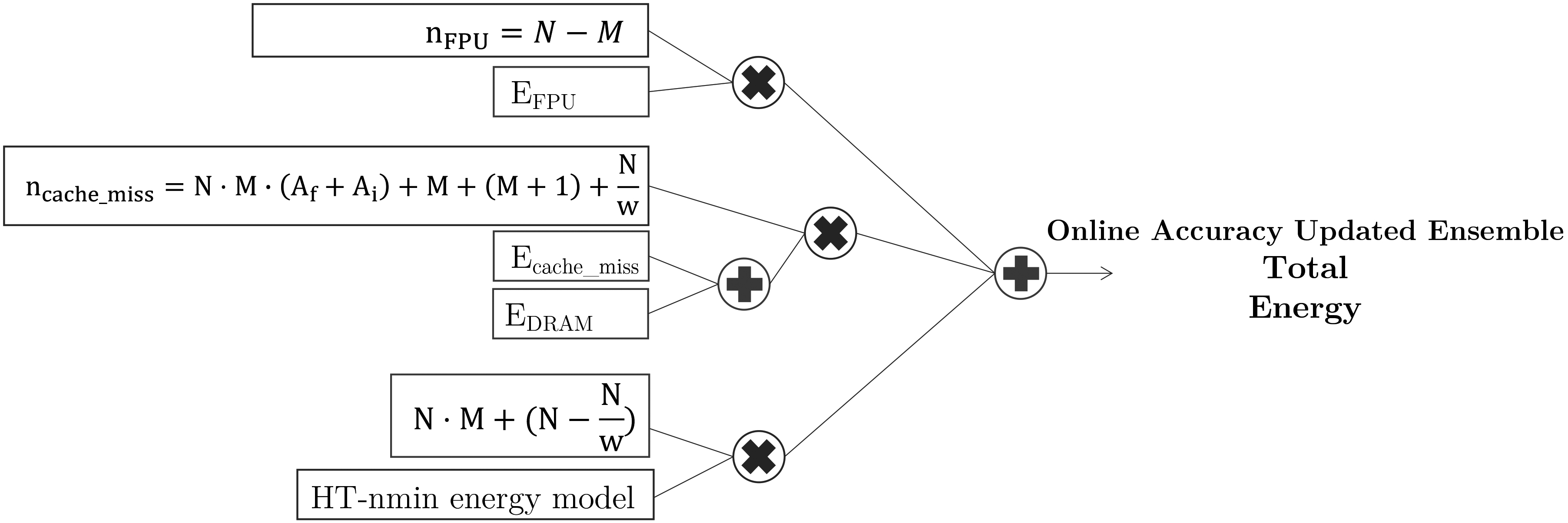
Regarding its energy consumption, we first present the main functions of the algorithm, to then present its energy patterns, combined in an energy model on Fig. 9. The main functions are: create a new classifier, calculate the prediction error, add classifier, weight classifier, and replace classifier.

• • Creating a new classifier requires one cache miss every w instances (lines 5 and 12), thus Nw.

• • Calculating the prediction error is the same energy as traversing the tree, that as previously explained for the HT-nmin and the Leveraging Bagging algorithms is one cache miss per attribute per instance (line 4), per model.

• • Adding a new classifier (line 7) is one cache miss every w instances, only the first M times.

• • Calculating the weight for each classifier requires one floating point operation per classifier per N-Nw instances, using the Eq. (8) on line 9, and then on line 15 for the rest of the instances. Thus it requires N floating point operations minus M (condition on line 6).

• • Replacing the classifier is the same as the function used in ADWIN, one cache miss per classifier to calculate the error for each classifier, plus one extra cache miss to replace it. This occurs for every Nw instances.

(8)

wit=1M⁢S⁢Ert+M⁢S⁢Eit+ε

5.Experimental design

We have performed several experiments to evaluate our proposed method, nmin adaptation, in ensembles of Hoeffding trees. The experiments have a dual purpose: i) first, to see how much energy consumption is reduced by applying the nmin adaptation method in ensembles of Hoeffding trees; ii) and second, to see how much accuracy is affected in case of this energy reduction. To fulfill those purposes, we have run a set of five different ensemble algorithms of Hoeffding trees, with and without nmin adaptation, and compared their energy consumption and accuracy. We have tested these algorithms over six synthetic datasets and five real world datasets, described in Table 1.

The ensembles used for this paper are: LeveragingBag, OCBoost, OnlineAccuracyUpdatedEnsemble, OzaBag, and OzaBoost. They have already been described in Section 4. All of them use the Hoeffding tree as the base classifier, with and without the nmin adaptation method.

The next subsections explain the datasets in more detail, together with the framework and tools for running the algorithms and measuring the energy consumption.

6.Results and discussion

The accuracy and energy consumption results of running algorithms LeveragingBag, OCBoost, OnlineAccuracyUpdatedEnsemble, OZaBag, and OzaBag, on the datasets from Table 1, are presented in Tables 2 and 3, respectively.

Figure 10.

Accuracy comparison between running the algorithms with and without nmin adaptation on all datasets. The results of each dataset are averaged for all algorithms.

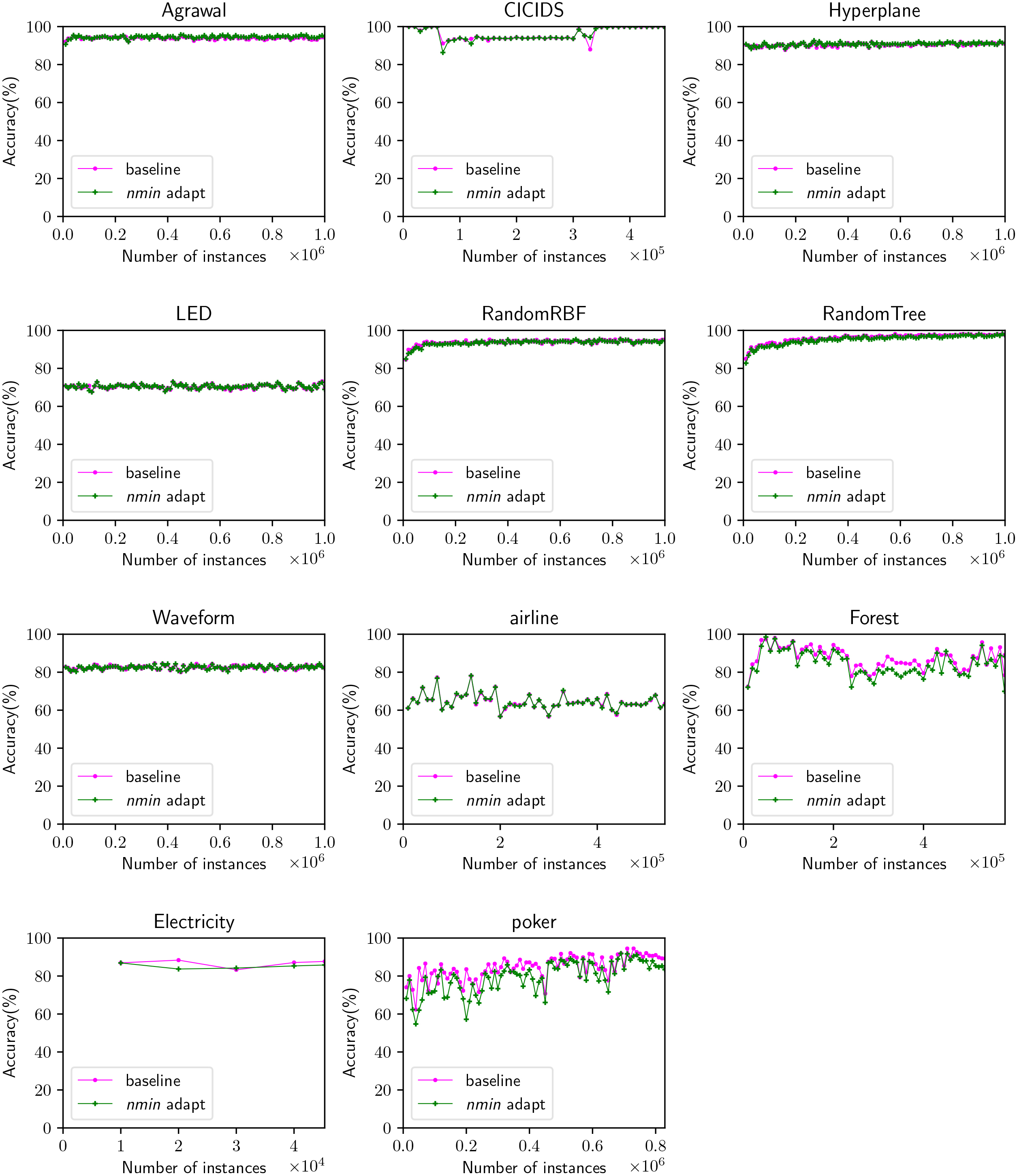
Figure 11.

Energy consumption for all datasets and all algorithms, with and without nmin adaptation.

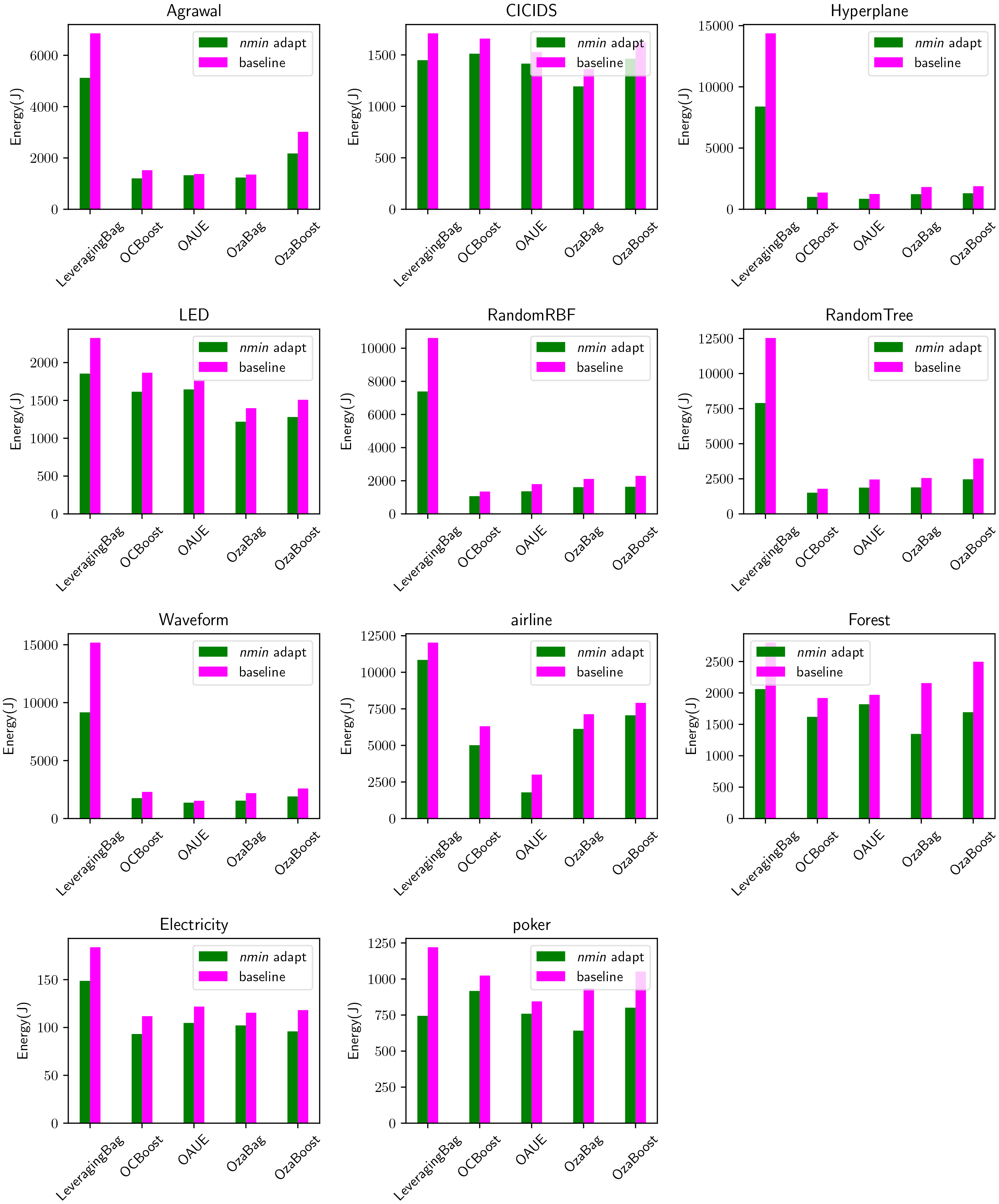
Figure 12.

Energy consumption and accuracy comparison for each algorithm, averaged for all datasets and for the nmin adaptation and baseline setups.

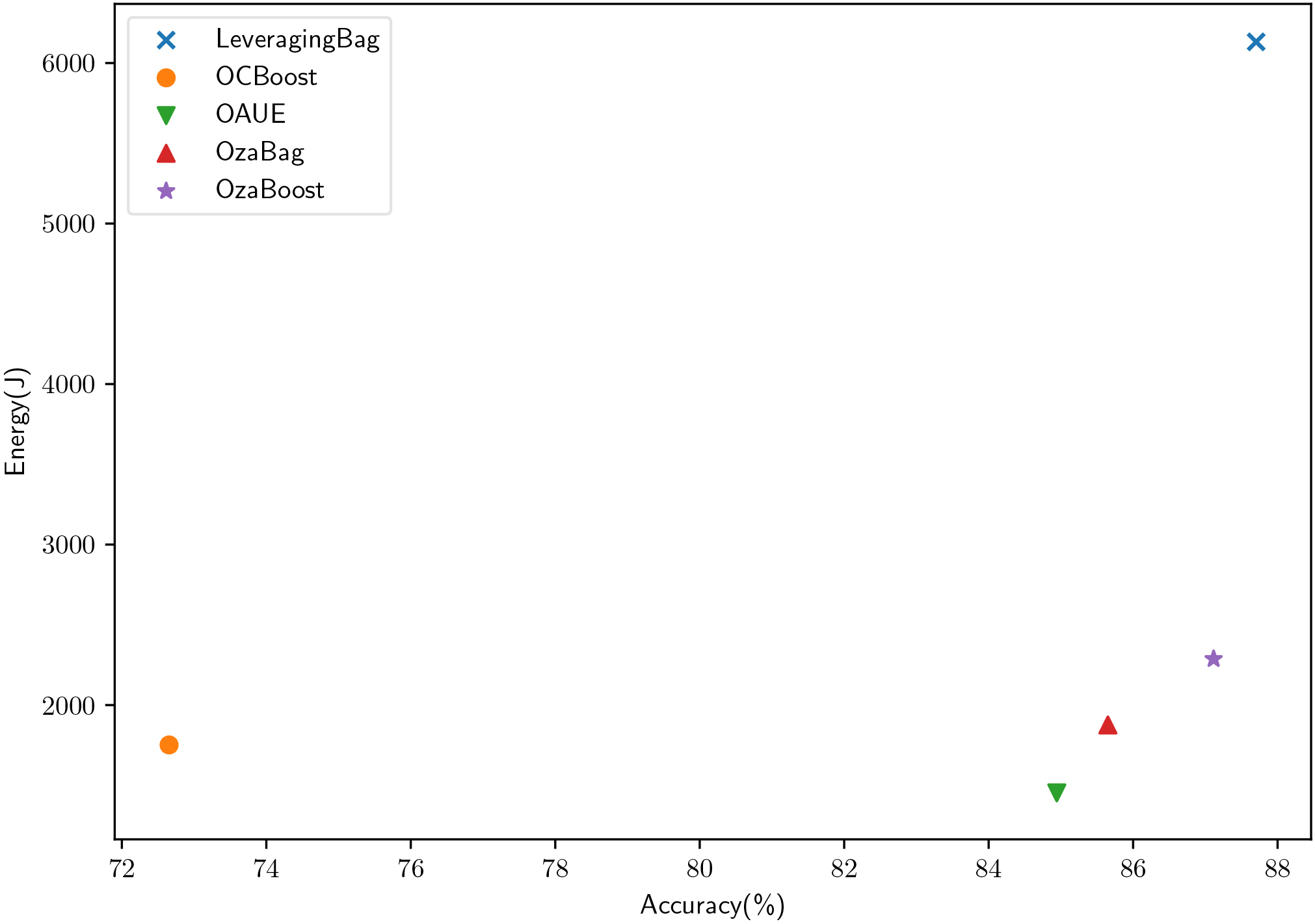
Table 4 presents the difference in accuracy and energy consumption between running the algorithm with and without nmin adaptation, our proposed method. The column Δ% details the difference, in percentage, between the accuracy of running the algorithm with and without nmin adaptation. A negative value represents that the algorithm with nmin adaptation obtained lower accuracy than the algorithm with the original implementation. The column Δ⁢(J) presents the difference, in percentage, between the energy consumption of running the algorithm with and without nmin adaptation. The lower the value the better, since it means that we reduced the energy consumption by that amount.

Looking at Table 4, we can see how for all algorithms and for all datasets nmin adaptation reduced the energy consumption by 21 percent, up to a 41 percent. Accuracy is affected by less than 1 percent on average. The poker dataset obtained the highest difference in accuracy between both methods, up to a 10 percent. However, the other datasets show how the original ensembles of Hoeffding trees and the version with nmin adaptation are comparable in terms of accuracy.

Figure 10 shows how accuracy increases with the number of instances. Each subplot represents all algorithms averaged for that particular dataset. Our goal with this figure is to show the difference between running the ensembles with and without nmin adaptation in terms of accuracy. We can observe how for most of the datasets (Agrawal, Hyperplane, LED, RandomRBF, RandomTree, Waveform, and airline) the difference is indiscernible, suggesting that the algorithm performs equally well for both the nmin adaptation approach and the standard approach. For the poker and forest dataset, we can see how nmin adaptation obtains lower accuracy than the standard approach. This was also visible in Table 2.

Figure 11 shows the energy consumption per dataset, per algorithm, with and without nmin adaptation. This figure clearly shows how all algorithms with nmin adaptation consume less energy than the standard version. This occurs in all datasets, even in datasets where the accuracy is higher for the nmin adaptation approach (e.g. Agrawal dataset, OzaBoost algorithm).

At a first glance, and without analyzing the results in depth, one could think that a higher accuracy requires a higher energy cost. However, our results show that there is not a direct relationship between accuracy increase and an increase in energy consumption. This can be observed in Fig. 12, which shows a comparison between accuracy and energy, per algorithm, averaged for all datasets, for the nmin adaptation and baseline setups. Looking also at Table 4, for instance at the OzaBoost algorithm, we can see how there is a high energy decrease (30 percent for the Hyperplane dataset) while still obtaining a higher accuracy (0.39 percent). Another algorithm with a high energy decrease is the OAUE for the airline dataset, where we decrease 40% the energy and accuracy is affected by 0.14 percent. A similar energy reduction is obtained in the poker dataset, for the LeveragingBag algorithm. However in this case the accuracy is significantly affected by 10%. These results are very promising, since they suggest that there is not a correlation between energy consumption and accuracy. Thus, there are ways, such as our current approach, to reduce the energy consumption of an algorithm without having to sacrifice accuracy. The importance lies on finding those hotspots that make the algorithm consume energy inefficiently.

In overall, our results show how nmin adaptation is able to reduce the energy consumption by 21 percent on average, affecting accuracy by less than one percent on average. This demonstrates that our solution is able to create more energy efficient ensembles of Hoeffding trees trading off less than one percent of accuracy.

7.Conclusions

This paper presents a simple, yet effective approach to reduce the energy consumption of ensembles of Hoeffding tree algorithms. This method, nmin adaptation, estimates the batch size of instances needed to check for a split, individually for each node. Thus, allowing the Hoeffding tree to grow faster in those branches where the confidence for choosing the best attribute is higher, and delaying the split in those branches where the confidence is lower.

We also present a generic approach to build theoretical energy models for any class of algorithms, together with energy models for the ensembles of Hoeffding trees used in this paper.

We conduct a set of experiments where we compare the accuracy and energy consumption of five ensembles of Hoeffding trees with and without nmin, on 11 publicly available datasets. The results show that nmin adaptation reduces the energy consumption significantly, on all datasets (up to a 41%, with 21% on average). This is achieved by trading off a few percentages of accuracy (up to a 10% for one particular dataset, on average of less than 1%). Our results also show that there is no clear correlation between a higher accuracy and a higher energy consumption. Thus, opening the possibility for more research to create more energy efficient algorithms without sacrificing accuracy.

While data stream mining approaches are focused on running on edge devices, still there has not been much research that tackle the energy efficiency of the approaches, which is a key variable for these devices. This study provides one step forward into achieving more energy efficient algorithms that are able to run in embedded devices. For future work, we plan on designing more energy efficient Hoeffding trees that are able to compete with high accurate current approaches[32].

References

[1] | R. Agrawal, T. Imielinski and A. Swami, Database mining: A performance perspective, IEEE Transactions on Knowledge and Data Engineering 5: (6) ((1993) ), 914–925. |
[2] | Y. Ben-Haim and E. Tom-Tov, A streaming parallel decision tree algorithm, Journal of Machine Learning Research 11: (Feb (2010) ), 849–872. |
[3] | A. Bifet and R. Gavalda, Learning from time-changing data with adaptive windowing, In Proceedings of the 2007 SIAM international conference on data mining, SIAM, (2007) , pp. 443–448. |
[4] | A. Bifet and R. Gavaldà, Adaptive learning from evolving data streams, In International Symposium on Intelligent Data Analysis, Springer, (2009) , pages 249–260. |
[5] | A. Bifet, G. Holmes, R. Kirkby and B. Pfahringer, Moa: Massive online analysis, Journal of Machine Learning Research 11: (May (2010) ), 1601–1604. |
[6] | A. Bifet, G. Holmes and B. Pfahringer, Leveraging bagging for evolving data streams, In Joint European conference on machine learning and knowledge discovery in databases, Springer, (2010) , pp. 135–150. |
[7] | A. Bifet, G. Holmes, B. Pfahringer, R. Kirkby and R. Gavaldà, New ensemble methods for evolving data streams, In Proceedings of the 15th ACM SIGKDD International Conference on Knowledge Discovery and Data Mining, Paris, France, June 28–July 1 2009, (2009) , pp. 139–148. |
[8] | A. Bifet, J. Zhang, W. Fan, C. He, J. Zhang, J. Qian, G. Holmes and B. Pfahringer, Extremely fast decision tree mining for evolving data streams, In Proceedings of the 23rd ACM SIGKDD International Conference on Knowledge Discovery and Data Mining, ACM, (2017) , pp. 1733–1742. |
[9] | L. Breiman, Bagging predictors, Machine Learning 24: (2) ((1996) ), 123–140. |
[10] | L. Breiman, Classification and regression trees, Routledge, (2017) . |
[11] | D. Brzeziński and J. Stefanowski, Accuracy updated ensemble for data streams with concept drift, In International conference on hybrid artificial intelligence systems, Springer, (2011) , pp. 155–163. |
[12] | D. Brzezinski and J. Stefanowski, Combining block-based and online methods in learning ensembles from concept drifting data streams, Information Sciences 265: ((2014) ), 50–67. |
[13] | Y.-H. Chen, T. Krishna, J.S. Emer and V. Sze, Eyeriss: An energy-efficient reconfigurable accelerator for deep convolutional neural networks, IEEE Journal of Solid-State Circuits 52: (1) ((2017) ), 127–138. |
[14] | H. David, E. Gorbatov, U.R. Hanebutte, R. Khanna and C. Le, Rapl: memory power estimation and capping, In Proceedings of the 16th ACM/IEEE international symposium on Low power electronics and design, (2010) , pp. 189–194. |
[15] | D. Dheeru and E. Karra Taniskidou, UCI machine learning repository, (2017) . |
[16] | P. Domingos and G. Hulten, Mining high-speed data streams, In Proc. 6th SIGKDD International Conference on Knowledge discovery and data mining, (2000) , pp. 71–80. |
[17] | Y. Freund and R.E. Schapire, A decision-theoretic generalization of on-line learning and an application to boosting, In Computational Learning Theory, Second European Conference, EuroCOLT ’95, Barcelona, Spain, March 13–15 1995, Proceedings, (1995) , pp. 23–37. |
[18] | E. García-Martín, N. Lavesson, H. Grahn, E. Casalicchio and V. Boeva, Hoeffding trees with nmin adaptation, In 2018 IEEE International Conference on Data Science and Advanced Analytics (DSAA), (2018) . |
[19] | K. Gauen, R. Rangan, A. Mohan, Y.-H. Lu, W. Liu and A.C. Berg, Low-power image recognition challenge, In Design Automation Conference (ASP-DAC), 2017 22nd Asia and South Pacific, IEEE, (2017) , pp. 99–104. |
[20] | S. Han, H. Mao and W.J. Dally, Deep compression: Compressing deep neural networks with pruning, trained quantization and huffman coding, In International Conference on Learning Representations (ICLR), (2016) . |
[21] | S. Han, J. Pool, J. Tran and W. Dally, Learning both weights and connections for efficient neural network, In Advances in neural information processing systems, (2015) , pp. 1135–1143. |
[22] | M. Harries, Splice-2 comparative evaluation: Electricity pricing, Technical report, The University of New South Wales, (1999) . |
[23] | J.L. Hennessy and D.A. Patterson, Computer architecture: a quantitative approach, Elsevier, (2011) . |
[24] | W. Hoeffding, Probability inequalities for sums of bounded random variables, Journal of the American Statistical Association 58: (301) ((1963) ), 13–30. |
[25] | M. Horowitz, 1.1 computing’s energy problem (and what we can do about it), In Solid-State Circuits Conference Digest of Technical Papers (ISSCC), 2014 IEEE International, IEEE, (2014) , pp. 10–14. |
[26] | G. Hulten, L. Spencer and P. Domingos, Mining time-changing data streams, In Proceedings of the seventh ACM SIGKDD international conference on Knowledge discovery and data mining, ACM, (2001) , pp. 97–106. |
[27] | E. Ikonomovska, Datasets, Retrieved from http://kt.ijs.si/elena_ikonomovska/data.html, 2013. Online; accessed 1 August 2018. |
[28] | J.G. Koomey, S. Berard, M. Sanchez and H. Wong, Assessing trends in the electrical efficiency of computation over time, IEEE Annals of the History of Computing 17: ((2009) ). |
[29] | N. Kourtellis, G.D.F. Morales, A. Bifet and A. Murdopo, Vht: Vertical hoeffding tree, In Big Data (Big Data), 2016 IEEE International Conference on, IEEE, (2016) , pp. 915–922. |
[30] | V. Losing, B. Hammer and H. Wersing, KNN classifier with self adjusting memory for heterogeneous concept drift, In IEEE 16th International Conference on Data Mining (ICDM), Dec (2016) , pp. 291–300. |
[31] | V. Losing, H. Wersing and B. Hammer, Enhancing very fast decision trees with local split-time predictions, In 2018 IEEE International Conference on Data Mining (ICDM), IEEE, (2018) , pp. 287–296. |
[32] | C. Manapragada, G. Webb and M. Salehi, Extremely fast decision tree, In Proceedings of the seventh ACM SIGKDD international conference on Knowledge discovery and data mining, ACM, (2018) . |
[33] | D. Marrón, E. Ayguadé, J.R. Herrero, J. Read and A. Bifet, Low-latency multi-threaded ensemble learning for dynamic big data streams, In Big Data (Big Data), 2017 IEEE International Conference on, IEEE, (2017) , pp. 223–232. |
[34] | N.C. Oza, Online bagging and boosting, In 2005 IEEE international conference on systems, man and cybernetics, volume 3, Ieee, (2005) , pp. 2340–2345. |
[35] | N.C. Oza and S. Russell, Experimental comparisons of online and batch versions of bagging and boosting, In Proceedings of the seventh ACM SIGKDD international conference on Knowledge discovery and data mining, ACM, (2001) , pp. 359–364. |
[36] | N.C. Oza and S. Russell, Online bagging and boosting, In In Artificial Intelligence and Statistics 2001, Morgan Kaufmann, (2001) , pp. 105–112. |
[37] | R. Pelossof, M. Jones, I. Vovsha and C. Rudin, Online coordinate boosting, In Computer Vision Workshops (ICCV Workshops), 2009 IEEE 12th International Conference on, IEEE, (2009) , pp. 1354–1361. |
[38] | C.F. Rodrigues, G. Riley and M. Luján, Fine-grained energy profiling for deep convolutional neural networks on the jetson tx1, In Workload Characterization (IISWC), 2017 IEEE International Symposium on, IEEE, (2017) , pp. 114–115. |
[39] | C.F. Rodrigues, G. Riley and M. Luján, Synergy: An energy measurement and prediction framework for convolutional neural networks on jetson tx1, In International Conference on Parallel and Distributed Processing Techniques and Applications, CSREA Press, (2018) , pp. 375–382. |
[40] | I. Sharafaldin, A.H. Lashkari and A.A. Ghorbani, Toward generating a new intrusion detection dataset and intrusion traffic characterization, In ICISSP, (2018) , pp. 108–116. |