


INTRODUCTION
Interrelations between ocean surface water, atmosphere, and continental environments play a key role in understanding mechanisms and causes of environmental change in terrestrial ecosystems. For the European continent, the North Atlantic Ocean represents the main source of humidity and precipitation (Trigo et al., Reference Trigo, Osborn and Corte-Real2002), and stipulated temperatures and general climate configurations during the Quaternary (Rahmstorf, Reference Rahmstorf2002; Rousseau et al., Reference Rousseau, Sima, Antoine, Hatté, Lang and Zöller2007; Martin-Garcia, Reference Martin-Garcia2019; Pinto and Ludwig, Reference Pinto and Ludwig2020). A general relationship between reduced North Atlantic sea surface temperatures (SST) and colder climate conditions over the continent during glacial/stadial periods has been demonstrated based on vegetation reconstructed from analysis of deep-sea sediment cores along the Iberian margin (Roucoux et al., Reference Roucoux, de Abreu, Shackleton and Tzedakis2005; Sánchez Goñi et al., Reference Sánchez Goñi, Landais, Fletcher, Naughton, Desprat and Duprat2008, Reference Sánchez Goñi, Desprat, Fletcher, Morales-Molino, Naughton, Oliveira, Urrego and Zorzi2018; Margari et al., Reference Margari, Skinner, Tzedakis, Ganopolski, Vautravers and Shackleton2010). It has been shown that vegetation changes closely corresponded to the millennial-scale variability of Dansgaard-Oeschger (D-O) cycles, however, vegetation response to specific D-O warming events and subsequent Greenland interstadials (GI) varied across Europe, pointing to variable effects of different D-O events (Fletcher et al., Reference Fletcher, Sánchez Goñi, Allen, Cheddadi, Combourieu-Nebout, Huntley and Lawson2010; Sánchez Goñi et al., Reference Sánchez Goñi, Desprat, Fletcher, Morales-Molino, Naughton, Oliveira, Urrego and Zorzi2018; see also Torner et al., Reference Torner, Cacho, Moreno, Sierro, Martrat, Rodriguez-Lazaro and Frigola2019). On the other hand, Greenland stadials (GS) were generally linked with marine cold spells in the North Atlantic with severe effects on marine dynamics as well as on vegetation development, especially in SW Europe. In this context, Heinrich Events (HE) (Heinrich, Reference Heinrich1988; Broecker, Reference Broecker1994) that presumably strongly altered the thermohaline circulation as the main heat supplier to the NE Atlantic were related to the most drastic marine temperature drops during the last glacial period, with equally strong effects on continental environments in Iberia (Cacho et al., Reference Cacho, Grimalt, Pelejero, Canals, Sierro, Flores and Shackleton1999; Bard et al., Reference Bard, Rostek, Turon and Gendreau2000; Sánchez Goñi et al., Reference Sánchez Goñi, Turon, Eynaud and Gendreau2000; Moreno et al., Reference Moreno, Cacho, Canals, Grimalt, Sánchez-Goñi, Shackleton and Sierro2005; Roucoux et al., Reference Roucoux, de Abreu, Shackleton and Tzedakis2005; Salgueiro et al., Reference Salgueiro, Voelker, de Abreu, Abrantes, Meggers and Wefer2010). As noted by Ganopolski and Rahmstorf (Reference Ganopolski and Rahmstorf2001), marine cooling linked to HEs was most pronounced in the subtropical Atlantic instead of the northern Atlantic where conditions were already cold. At the Iberian margin, in addition to the detection of ice-rafted debris (IRD) and strong declines of North Atlantic SSTs, a dramatic decrease of thermophilous flora over the Iberian mainland has also been related to Heinrich stadials (HS; stadials comprising Heinrich Events, see, e.g., Sánchez Goñi and Harrison, Reference Sánchez Goñi and Harrison2010) (Turon et al., Reference Turon, Lézine and Denèfle2003; Roucoux et al., Reference Roucoux, de Abreu, Shackleton and Tzedakis2005). Given the close proximity to the North Atlantic, a strong effect of marine cold spells on terrestrial systems of the Iberian Peninsula should be expected, in particular when related to HEs. But apart from Iberian marine records and some findings mainly from the northern Iberian mainland (González-Sampériz et al., Reference González-Sampériz, Valero-Garcés, Moreno, Jalut, García-Ruiz, Martí-Bono, Delgado-Huertas, Navas, Otto and Dedoubat2006; Moreno et al., Reference Moreno, Stoll, Jiménez-Sánchez, Cacho, Valero-Garcés, Ito and Edwards2010; Vegas et al., Reference Vegas, Ruiz-Zapata, Ortiz, Galán, Torres, García-Cortés, Gil-García, Pérez-González and Gallardo-Millán2010; Ortiz et al., Reference Ortiz, Moreno, Torres, Vegas, Ruiz-Zapata, García-Cortés, Galán and Pérez-González2013), terrestrial records providing such indications are very rare (González-Sampériz et al., Reference González-Sampériz, Leroy, Fernández, García-Antón, Gil-García, Uzquiano, Valero-Garcés and Figueiral2010; Moreno et al., Reference Moreno, González-Sampériz, Morellón, Valero-Garcés and Fletcher2012). In this context, a major research gap exists for the central part of Iberia, which is characterized by a strong continental climate due to isolating effects of the framing mountain ranges. When effects of HEs on terrestrial systems on a global scale is considered (Ganopolski and Rahmstorf, Reference Ganopolski and Rahmstorf2001; Claussen et al., Reference Claussen, Ganopolski, Brovkin, Gerstengarbe and Werner2003; Pausata et al., Reference Pausata, Li, Wettstein, Kageyama and Nisancioglu2011; Thomas et al., Reference Thomas, Burrough and Parker2012; Han et al., Reference Han, Li, Yi, Stevens, Chen, Wang and Lu2015; Xiong et al., Reference Xiong, Li, Chang, Algeo, Clift, Bretschneider and Lu2018), the Iberian interior seems to be particularly suitable to examine whether relations between terrestrial system behavior and marine cold spells (and HEs in particular) can be established in regions linked to certain continentality. In that regard, observations have been hampered so far by the absence of appropriate archives.
The upper Tagus Basin (Fig. 1) is part of the Iberian Southern Meseta and is characterized by vast deposits of Tertiary gypseous and calcareous marls that have been intensely dissected during the Quaternary (Silva et al., Reference Silva, Roquero, López-Recio, Huerta and Martínez-Graña2017). This erosive environment generally prevented the preservation of sedimentary sequences during the Pleistocene except for fluvial deposits (Panera et al., Reference Panera, Torres, Pérez-González, Ortiz, Rubio-Jara and Uribelarrea del Val2011; Silva et al., Reference Silva, López-Recio, Tapias, Roquero, Morín, Rus, Carrasco-García, Giner-Robles, Rodríguez-Pascua and Pérez-López2013; Wolf et al., Reference Wolf, Seim, Diaz del Olmo and Faust2013; Wolf and Faust, Reference Wolf and Faust2015; Wolf and Faust, Reference Wolf and Faust2016; Moreno et al., Reference Moreno, Duval, Rubio-Jara, Panera, Bahain, Shao, Pérez-González and Falguères2019), which reveal an incomplete record of the last glacial period. Continuous pollen records exist almost exclusively in higher altitudes of the Spanish Central System (Sierra des Gredos and Sierra de Guadarrama) and the Iberian Range, and are temporally restricted to the time after mountain glaciers retreated in the course of Marine Isotope Stage (MIS) 2 (Turu et al., Reference Turu, Carrasco, Pedraza, Ros, Ruiz-Zapata, Soriano-López and Mur-Cacuho2018). Glacial landforms provide valuable information on glacier advances and retreats in the Spanish Central System (SCS; Palacios et al., Reference Pausata, Li, Wettstein, Kageyama and Nisancioglu2011, Reference Palacios, de Andrés, de Marcos and Vázquez-Selem2012; Domínguez-Villar et al., Reference Domínguez-Villar, Carrasco, Pedraza, Cheng, Edwards and Willenbring2013; Carrasco et al., Reference Carrasco, Pedraza, Domínguez-Villar, Willenbring and Villa2015) that correlate with main environmental changes in the high mountain area. However, because glacier growth strongly depends on both cold temperatures and sufficient moisture availability (Domínguez-Villar et al., Reference Domínguez-Villar, Carrasco, Pedraza, Cheng, Edwards and Willenbring2013), the glacial record is largely insensitive to the most arid stages of the last glacial period. Also, the last glacial maximum (LGM) advance has generally overtaken deposits of older and less intensive glacier advances.

Figure 1. In the left portion of the figure, location of the study area in the center of the Iberian Peninsula indicated by red square; Eagle Cave in the Gredos Range indicated by black star (SCS, Domínguez-Villar et al. Reference Domínguez-Villar, Carrasco, Pedraza, Cheng, Edwards and Willenbring2013); locations of deep ocean sediment cores MD95-2042 and SU81-18 indicated by black stars in the Atlantic Ocean off the Iberian margin (Sánchez Goñi et al., Reference Sánchez Goñi, Turon, Eynaud and Gendreau2008). In the right portion of the figure, distribution of loess deposits is indicated in orange (following the geological map by de San José, Reference De San José Lancha1973); studied sections are marked by yellow triangles. (For interpretation of references to color in this figure caption, the reader is referred to the web version of this article.)
Another area of the Southern Meseta, specifically the upper catchment of the Guadiana River south of the Montes de Toledo (Fig. 1), is characterized by having had less intense surface erosion during the late Quaternary due to a higher local base level of erosion. Here, the wetlands of the upper Guadiana River represent a valuable Late Pleistocene archive that is being intensively researched (e.g., Santisteban et al., Reference Santisteban, Mediavilla, Galán de Frutos and López Cilla2019). The sedimentary record of the Fuentillejo maar lake in the volcanic field of Campo de Calatrava (Ortiz et al., Reference Ortiz, Moreno, Torres, Vegas, Ruiz-Zapata, García-Cortés, Galán and Pérez-González2013) shows evidence of environmental fluctuations corresponding to D-O cycles. More specifically, Vegas et al. (Reference Vegas, Ruiz-Zapata, Ortiz, Galán, Torres, García-Cortés, Gil-García, Pérez-González and Gallardo-Millán2010) found cold and arid conditions related to HE 2, HE 1, and the Younger Dryas, whereas HEs 3–5 were assumed to relate to rather warm and arid conditions. However, relatively low chronological resolution was the limiting factor here. Finally, there are numerous playa lakes in the Southern Meseta (Schütt, Reference Schütt2000). However, due to high salinity and frequent desiccation events, these lake sediments revealed a limited potential in recording last glacial paleoenvironmental evolution.
From this, it follows that reliable information about the effect of marine cold spells linked to stadial phases on geomorphological systems in central Iberia is lacking, even more if stadials comprising HEs (HS) are considered. Hence, there is a need for systematic studies on fluvial, aeolian, and glacial sedimentary archives relating to relevant past earth surface processes. In order to meet this need and to verify whether Greenland stadials as well as Heinrich stadials exercised a decisive influence on geomorphological systems, we undertook comprehensive studies on loess deposits in the upper Tagus Basin to obtain a more complete picture of late Pleistocene landscape dynamics in central Spain. Besides a general evaluation of phases linked to loess deposition and surface stability, we used a broad multi-proxy approach in order to accurately characterize hydrological conditions, paleotemperatures, and wind strengths during the last glacial period.
METHODS
Stratigraphic work
In total, five loess sections were included in this study in order to obtain a representative composite profile for the last glacial period (Fig. 1). All sections were analyzed in the field, including differentiation of sedimentary units, the presence of paleosols or processes indicating soil formation, and evidence for relocation processes. We took samples from all sections for laboratory analyses. In general, sampling was oriented towards stratigraphic layers with the aim of providing a representative record of all dynamic phases during the last glacial period. On average, samples for standard analyses were taken at ~15 cm intervals from all sections. We took 28 samples for heavy mineral analyses from each layer in three sections (Fuentidueña, Paraíso, and A3). We also took seven samples from surrounding areas (for more details, see Wolf et al., Reference Wolf, Ryborz, Kolb, Calvo Zapata, Sanchez Vizcaino, Zöller and Faust2019). The same three sections sampled for heavy mineral analysis were also chosen for luminescence dating on 25 samples. The most complete section (Paraíso) was sampled for n-alkane biomarker analyses and stable isotope measurements, with 25 samples with an average sampling density of 25 cm taken.
Standard analyses
Grain-size determination was conducted by pipette analyses and wet sieve techniques (Schlichting et al., Reference Schlichting, Blume and Stahr1995) after dispersion with sodium pyrophosphate. Because samples contained gypsum that disrupted the settling process in the sample cylinder by flocculation, all samples were passed through a repeated cycle of dissolution and centrifugation until measured electrical conductivity fell below a value of 400 μS cm−3 (Frenkel et al., Reference Frenkel, Gerstl and van de Veen1986). For determining fraction-specific carbonate contents for different grain-size classes, we conducted grain-size analysis twice, with a first run implemented without decalcification, and a second run after carbonates were dissolved using 10% HCl. Following this procedure, a particle size index (PSI) was calculated based on samples that were not decalcified by forming a ratio between the coarse silt/fine sand fractions (> 20 μm and < 200 μm) and all finer fractions, including medium silt, fine silt, and clay. The calcium carbonate content was determined by measuring the carbon dioxide gas volume after adding hydrochloric acid in a Scheibler apparatus (Schlichting et al., Reference Schlichting, Blume and Stahr1995). Soil organic matter was measured via suspension and catalytic oxidation (TOC-VCPN/DIN ISO 16904). Total iron content (Fe(t)-values) was determined after pressure digestion with concentrated nitric and hydrofluoric acid using atomic adsorption spectrometry (Analytic Jena, Vario 6). Pedogenic iron content (Fe(d)-values) was measured after dithionite extraction using atomic adsorption spectrometry (Schlichting et al., Reference Schlichting, Blume and Stahr1995). The ratio between pedogenic and total iron may provide information of the intensity of weathering, and thus may indicate soil formation in the case of higher values in comparison to the parent material.
Micromorphological analyses
For micromorphological analyses, 18 oriented and undisturbed samples were collected from selected horizons of the sequences at Paraíso and Fuentidueña. Vertical thin sections were prepared at the Laboratory of Soil Science and Geoecology at the Institute of Geography, Eberhard-Karls-University, Tübingen. Thin sections were then analyzed and photographed using a polarizing microscope (Zeiss Axiovision). Thin section descriptions mainly are based on the terminology after Bullock et al. (Reference Bullock, Fedoroff, Jongerius, Stoops and Tursina1985) and Stoops (Reference Stoops2003).
Age determination: luminescence dating
Optically stimulated luminescence (OSL) measurements were applied to the coarse-grained quartz fraction (90–200 μm). Following standard procedures (e.g., Fuchs et al., Reference Fuchs, Fischer and Reverman2010), sample preparation was performed under subdued red-light conditions (640 ± 20 nm), including wet sieving, removal of carbonates and organic material, and a density separation using sodium polytungstate. We etched the quartz separates in 40% HF for 50 minutes.
For OSL measurement, quartz grains were mounted on aluminum cups, using a 3-mm mask that restricted the number of grains to ~100–300 grains per disc. Except for samples HUB 470, HUB 471, and HUB 472, which were measured at the Humboldt University in Berlin, all luminescence measurements were carried out at the University of Bayreuth using an automated Risø-Reader TL/OSL-DA-15 equipped with a 90Y/90Sr β-source for artificial irradiation. Blue LEDs (470 ± 30 nm) were used for OSL stimulation, and the luminescence signal was detected by a Thorn-EMI 9235 photomultiplier combined with a 7.5 mm U-340 Hoya filter (290–370 nm).
All luminescence shine-down curves were recorded for 40 seconds at an elevated temperature of 125°C, using a single aliquot regenerative-dose (SAR) protocol (Murray and Wintle, Reference Murray and Wintle2000), which was enhanced by an additional hot-bleach step (Murray and Wintle, Reference Murray and Wintle2003). Equivalent doses were determined using the first 0.6 seconds of the OSL signal after subtracting a background that was derived from the last 7.5 seconds.
Only aliquots with a recycling ratio of 0.9–1.1, a recuperation of ≤ 5% of the natural sensitivity corrected signal intensity (Murray and Wintle, Reference Murray and Wintle2000), and an OSL-IR depletion ratio (Duller, Reference Duller2003) in the range of 0.9–1.1 were accepted for equivalent dose calculation. Because dose response curves of some samples (BT 1368, BT 1372, BT 1374, BT 1376, BT 1383, BT 1384, and HUB 470) suggested that these samples might be close to their saturation levels, we would like to emphasize that all ages derived from these samples may seriously underestimate the true burial age and can only be interpreted as minimum ages.
For dose rate (Ḋ) determination, the U- and Th-concentrations were detected by thick source α-counting, and the K-contents were measured by ICP-OES. Calculations for determining the environmental dose rate were done applying DRAC v1.2 (Durcan et al., Reference Durcan, King and Duller2015) in combination with the conversion factors given by Guérin et al. (Reference Guérin, Mercier and Adamiec2011). Applying an interstitial water content of 8 ± 3% for samples BT 1375, BT 1381, BT 1383, BT 1384, and BT 1544, a water content of 5 ± 3% was assumed to be representative for all other samples as derived from measurements of present-day water contents and considering both sedimentological properties and differences in the geographical settings of the locations. Cosmic dose rates were calculated according to Prescott and Hutton (Reference Prescott and Hutton1994) using the ‘calc_CosmicDoseRate’ function provided by the R package ‘Luminescence’ (Kreutzer et al., Reference Kreutzer, Schmidt, Fuchs, Dietze, Fischer and Fuchs2012, Reference Kreutzer, Dietze, Burow, Fuchs, Schmidt, Fischer and Friedrich2016; R Development Core Team, 2016).
Heavy mineral analyses
The separation of heavy minerals was conducted after the procedure described by Mange and Maurer (Reference Mange and Maurer1991), including drying the samples, sieving to a grain-size fraction between 40 μm and 400 μm, removal of carbonates by adding acetic acid, eliminating gypsum by repeated soaking and sieving, and dispersing with Na4P2O7. Finally, the heavy mineral fraction was separated by using sodium polytungstate. For the identification of the heavy minerals, we produced strewn slides after Kurze (Reference Kurze1987) for transmitted light microscopy by coating with gelatin, and unilateral embedding in the immersion fluid α-chloronaphtalene with a light refraction of 1.633. For optimal analyses, we identified and counted at least 200 translucent mineral grains. Determination of the identity of translucent minerals was based on grain morphologies, colors, pleochroism features, fissility, break, light refraction, double refraction, as well as inclusions (for details, see Wolf et al., Reference Wolf, Ryborz, Kolb, Calvo Zapata, Sanchez Vizcaino, Zöller and Faust2019).
Rock magnetic measurements
Magnetic susceptibility was measured on two different frequencies (300 and 3000 Hz) using the MAGNON VFSM susceptibility bridge (320 Am−1 AC field, sensitivity greater than 5 x 10⁻⁶ SI) and transferred to mass specific susceptibility χ after determining sample density. The frequency dependent susceptibility (χfd) was calculated using the difference of both measured frequencies. The isothermal remanent magnetisation (IRM) was generated employing a MAGNON Pulse Magnetiser II with fields of 2000 mT and 200 mT (backfield) and resulting imposed magnetic remanences were determined using an AGICO JR6-spinner magnetometer. The s-ratio was calculated based on both values (s-ratio = ((IRM200 mT/IRM2000 mT) + 1)/2).
Stable isotope analyses
In order to reconstruct paleoclimatic and paleohydrological changes, we performed compound-specific stable isotope analyses of δ13C and δ2H on the aliphatic lipid fraction containing n-alkanes. The δ13C signal of leaf waxes can be used to distinguish between C3 and C4 vegetation (Rommerskirchen et al., Reference Rommerskirchen, Eglinton, Dupont and Rullkötter2006), with C3 plants showing lower values (−23‰ to −34‰) compared to C4 plants (−6‰ to −23‰, Schidlowski, Reference Schidlowski1987). Additionally, the δ13C value of leaf wax n-alkanes depends on the δ13C of the atmospheric CO2, as well as on its concentration, air temperature, relative humidity, and precipitation during the growing season (e.g., Diefendorf et al., Reference Diefendorf, Mueller, Wing, Koch and Freeman2010). The δ2H values of leaf waxes reflect the isotopic signal of the precipitation, which depends mainly on the isotopic composition of the moisture source, but is also influenced by the temperature, amount, continentality, and altitude effect (Berke et al., Reference Berke, Tipple, Hambach and Ehleringer2015; Sachse et al., Reference Sachse, Billault, Bowen, Chikaraishi, Dawson, Feakins and Freeman2012; Tipple et al., Reference Tipple, Berke, Doman, Khachaturyan and Ehleringer2013). Because we assume that δ2Hwax variations in the upper Tagus loess correspond to changes in δ18O in the North Atlantic surface waters, thus indicating that the source effect was one dominant control on δ2Hwax (Schäfer et al., Reference Schäfer, Bliedtner, Wolf, Kolb, Zech, Faust and Zech2018), here we focus solely on δ13C as proxy for hydrological changes.
Total lipid extraction and separation into lipid fractions is described in Schäfer et al. (Reference Schäfer, Bliedtner, Wolf, Faust and Zech2016a). The compound-specific carbon isotope measurements were performed on an IsoPrime 100 mass spectrometer, coupled to an Agilent 7890A gas chromatograph via a GC5 Pyrolysis/Combustion interface that operated in combustion mode (CuO reactor) at 850°C. Samples were injected using a split/splitless injector in splitless mode. The GC was equipped with a 30 m fused silica column (HP5-MS, 0.32 mm i.d., 0.25 μm film thickness). The precision was checked by injecting a standard alkane mix (C27, C29, C33) with known isotopic composition (Schimmelmann) twice every six runs. The analytical error was generally better than 0.5‰ (triplicate measurements). The stable carbon isotope composition is given in the delta notation (δ13C) versus Vienna Pee Dee Belemnite (V-PDB). For the compound-specific hydrogen isotope measurement, the GC5 mode was changed to pyrolysis by using a Cr (ChromeHD) reactor at 1000°C. Adjustments for the GC, the standard and the injection procedure were the same as for the stable carbon isotope measurements. The H3+ correction factor was checked every two days and was stable at 3.48 ± 0.06. The analytical error was generally better than 5‰ (three replicates), and we report only values with a standard deviation better than 6‰ (for more details, see Schäfer et al., Reference Schäfer, Bliedtner, Wolf, Kolb, Zech, Faust and Zech2018).
RESULTS
Lithofacies and pedostratigraphic patterns of the Upper Tagus loess record
The Upper Tagus loess record can be subdivided into 10 main stratigraphic units (SU-1 to SU-10). The basal two units contain the underlying substrates: Miocene marls (SU-1) and Middle Pleistocene fluvial gravel terraces (SU-2). Unit SU-3 is comprised of relocated material at the base of the sections, while SU-4 to SU-9 contain loess deposits that were formed during the last glacial period. Holocene colluvial deposits (SU-10) cover the top of most of sections. All stratigraphic columns together with standard analytical results are show in Figures 2–7. The Villamanrique section is strongly influenced by slope processes and also contains runoff channels in its upper part (Fig. 5E), indicating active surface dynamics during loess deposition.

Figure 2. (color online) Stratigraphic sequence and analytical data for the Fuentidueña section (40°05′14.76″N, 03°12′18.03″W; 560 m asl), showing OSL dating results, sediment units (SU), sampling points, palaeo surfaces (PS), grain-size parameters (soil texture %, coarse silt content % sand content %), organic content, carbonate content (total and coarse silt sized fractions), ratio between pedogenic and total iron as a weathering index, and results of rock magnetic measurements (magnetic susceptibility, frequency-dependent susceptibility, s-ratio). See key for detailed sedimentological features, pedogenic features, and kind of samples taken.

Figure 3. Fuentidueña section photographs and schematic stratigraphic sketch of cross-section. Insets with red lines in the stratigraphic sketch refer to photographs. Shovel (~60 cm) for scale in photos. (A) Lower part of the section is comprised of layered loamy soil sediments (SU-3) above fluvial gravels of mid- to late Pleistocene age (SU-2). (B) Photograph shows transition from the brownish sediments of SU-3 to loess deposits above. PS-1 marks the dark reddish paleosol that was formed in SU-4 and the lighter loess of SU-5. (C) Middle and upper part of the section. Above the intense PS-1, palaeo surface PS-3 appears much weaker. A whitish horizon with secondary carbonate enrichment is apparent at the base of SU-7. The strong boundary between SU-8 and SU-9 marks the limit of moisture penetration from the surface. (For interpretation of references to color in this figure caption, the reader is referred to the web version of this article.)

Figure 4. (color online) Stratigraphic sequence and analytical data for the A3 section (40°06′38.9″N, W 03°08′47.5″W; 560 m asl), showing OSL dating results, sediment units (SU), sampling points, palaeo surfaces (PS), and grain-size parameters (soil texture %, coarse silt content % sand content %), organic content, carbonate content (total and coarse silt-sized fractions), and ratio between pedogenic and total iron as a weathering index. For legend, see Figure 2.

Figure 5. (color online) Photographs of various loess sections with shovel for scale (~60 cm); schematic cross-section of the Villamanrique section. (A, B) Typical appearance of SU-3 in the Villamanrique section (B) and another section near the valley bottom (A); note alternation between dark-brown clayey deposits and the hardened laminar carbonate enrichments. (C) Lower and middle parts of the Paraíso section with indication of sediment units (SU) and palaeo surfaces (PS-1 to PS-3); note the whitish marls of SU-1 at base of the section. (D) Lower and middle part of the Villarubia section. The paleosol PS-1 shows less intense development compared to the other sections, and PS-3 has very weak features. (E) Schematic cross-section of the Villamanrique section (40°5′32.75″N, 3°11′29.46″W; 546 m asl). The outcrop is located at the bottom of a tributary valley and was strongly influenced by slope processes and surface runoff during the last glacial period as shown by the admixture of pebbles and coarse-grained sediments, a secondary fluvial channel-fill at the top of the sequence, and erosion discordances. Nevertheless, units SU-3 and SU-4 show features that are similar to those found in other sections, including the strong paleosol linked to PS-1.
Lower part of the sections (SU-2 and SU-3)
General topographic positions of the described loess sections are shown in Figures 1 and 8. The lower parts of the sections differ significantly in relation to their respective elevation above the recent river level. In the Fuentidueña (Figs. 2, 3), A3 (Fig. 4), and Villamanrique (Fig. 5) sections, which are elevated between 10–20 m above recent river level, the last glacial deposits rest on older fluvial terraces consisting of poorly sorted, well-rounded gravels and coarse-grained sand lenses (SU-2). The subsequent unit (SU-3) is characterized by a more than 2-m-thick succession of alternating layers of dark brown clayey sediments with clay contents of up to 55%, and sandy layers, some with more than 50% of fine and medium sand. Among the sandy and clayey layers, there are very thin, laminar, carbonate accumulations with carbonate contents of up to 66% that indicate precipitation from carbonate-saturated runoff (Fig. 5A, B). SU-3 lacks clear indications of in-situ soil formation. Instead, the high soluble salts and clay contents, and high values of magnetic susceptibility (Fig. 2), indicate that SU-3 mainly consists of relocated loamy soil material that was derived from surface erosion of the surrounding evaporate marls. Sedimentation features in these footslope positions are tentatively interpreted as a mixture of slope processes and fluvial sedimentation processes in a still-active floodplain environment.
In contrast to the sections at Fuentidueña and Villamanrique, loess and loess derivates of the Paraíso (Figs. 5C, 6) and Villarubia (Figs. 5D, 6, 7) sections, located 50 m and 93 m above recent river level (Fig. 8), rest directly on Miocene marls (SU-1). These marls are characterized by soluble salt contents between 48 and 78%, and carbonate contents between 9 and 29% (Figs. 6, 7). At the beginning of section accumulation, these more elevated areas were not influenced by floodplain processes, but rather were affected by erosive instead of depositional processes. Accordingly, in the Paraíso section, there is no indication of major SU-3 deposition apart from a thin layer of relocated marl deposits.
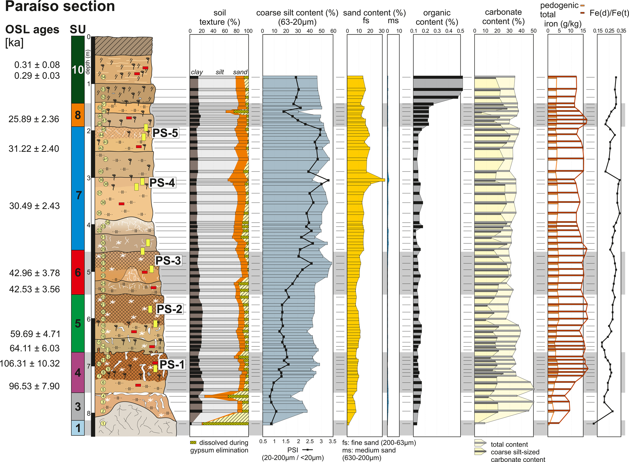
Figure 6. (color online) Stratigraphic sequence and analytical data for the Paraíso section (40°01′51.07′N', 03°28′01.70″W; 556 m asl), showing OSL dating results, sediment units (SU), sampling points, palaeo surfaces (PS), and grain-size parameters (soil texture %, coarse silt content % sand content %), organic content, carbonate content (total and coarse silt-sized fractions), and ratio between pedogenic and total iron as a weathering index. For legend, please see Figure 2.

Figure 7. (color online) Stratigraphic sequence and analytical data of the Villarubia section (40°01′42.2″N, 03°25′30.3″W; 607 m asl), showing sediment units (SU), sampling points, palaeo surfaces (PS), and grain-size parameters (soil texture %, coarse silt content % sand content %), organic content, carbonate content (total and coarse silt-sized fractions), and ratio between pedogenic and total iron as a weathering index. For legend, please see Figure 2.

Figure 8. (color online) Schematic sketch showing topographic positions of individual loess sections with respect to vertical (blue arrows) and horizontal (dark grey arrows) distances from the river floodplain/braid plain as dominant sediment source. Higher aeolian transport distances are accompanied by gradual sediment fining (decreasing % fS and mean grain-size) due to particle size-sorting (after Wolf et al., Reference Wolf, Ryborz, Kolb, Calvo Zapata, Sanchez Vizcaino, Zöller and Faust2019). Simplified figure; loess sections are not on a single transect. For actual section positions, please see Fig. 1. fS = fine sand
First indications of loess deposition (SU-4)
The next unit, SU-4, marks the beginning of the last glacial loess formation in the study area. Sediment samples show higher silt and fine sand contents, while sections located closer to the river level show generally higher sand contents (e.g., Fuentidueña) compared to sections in more elevated positions (Fig. 8).
These relations are well expressed in form of texture-related indices, such as the grain-size index (GSI) that compares coarse silt contents with all finer fractions, thus indicating wind strength in loess archives (Rousseau et al., Reference Rousseau, Antoine, Hatte, Lang, Zoller, Fontugne and Ben Othman2002). In view of the high fine sand contents (e.g., up to 27% in Fuentidueña section, Fig. 2), loess deposits appear to be mainly of local origin (see e.g., Bosq et al. Reference Bosq, Bertran, Degeai, Kreutzer, Queffelec, Moine and Morin2018). In order to consider the fine sand fraction for calculating a wind-strength-related proxy, we applied a new particle-size index (PSI = (20–200μm)/<20μm) which, besides coarse silt, also emphasizes fine sand (Calvo et al., Reference Calvo, Sanchez, Acosta, Wolf and Faust2016; Wolf et al., Reference Wolf, Ryborz, Kolb, Calvo Zapata, Sanchez Vizcaino, Zöller and Faust2019). In the Paraíso section, which is (along with the Villarubia section) the most suitable section for studying aeolian transport processes due to its distal position from the deflation area, the PSI rises to about 1.5 in SU-4 (Fig. 6), which is quite low compared to other loess units. Further sedimentological characteristics of SU-4 include the highest carbonate contents in all sections (Figs. 2, 6, 7), the highest content of medium and coarse sand in Fuentidueña (Fig. 2), and a scattered occurrence of angular, several-cm-thick stones or pebbles in Paraíso and Fuentidueña that indicate the contribution of slope processes during the formation of SU-4. In the upper part of SU-4, a strongly weathered paleosol (palaeo surface (PS) 1; Fig. 5C) shows a strong reddish ochre-brown color, bioturbation features, and numerous carbonate nodules as well as up to 15-cm-long carbonate concretions with rhizolith-like shapes. The paleosol (PS-1) exhibits maximum values of magnetic susceptibility and a peak in the Fe(d)/Fe(t)-ratio. However, the grain-size patterns require closer consideration. Generally, in all sections, ~30–70% of the silt and sand fraction are comprised of calcium carbonate minerals. The clay fraction shows a much lower percentage of carbonate, but in line with maximum values of the total carbonate content, it rises up to more than 50%, showing a sedimentary origin for the clay-sized carbonate minerals. Therefore, grain-size patterns appear to be suitable for analyzing sedimentation processes, but less suitable for detecting pedogenic processes. This can be seen, e.g., in the Paraíso section in SU-4, in which clay contents show higher values in the parent material as compared to the paleosol (Fig. 6), although it is the most intensely developed paleosol of the whole section. However, if we also consider clay contents measured after decalcification of the samples (Fig. 9), 37–54% of the clay below the paleosol consists of calcium carbonate minerals, while the paleosol itself also shows an increase of clay after decalcification. This may be due to the disaggregation of clay aggregates during decalcification or the release of clay from inside of secondary carbonate concretions. Finally, this paleosol shows the highest carbonate-free clay contents in the Paraíso and Villarubia sections.
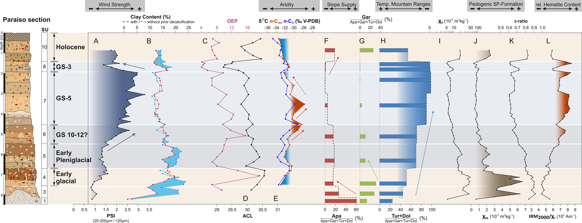
Figure 9. Results of extended analyses of the Paraíso section. Stratigraphic sketch includes general sampling points (yellow circles), positions of luminescence (red boxes) and heavy mineral samples (blue circles labeled SM), stratigraphic units (SU), and glacial and GS events. (A) Particle-size index (PSI; (fine sand + coarse silt)/(medium silt + fine silt + clay)), reflecting wind strength. Grey arrows indicate increasing/decreasing wind strength. (B) Clay content (upper scale) with (red line) and without (blue line) prior decalcification. (C) Odd-over-even predominance (OEP) of n-alkanes (light purple line and upper scale) as an indication of preservation (higher values imply better preservation). (D) Average chain length (ACL) of n-alkane homologues (black line and lower scale) (Schäfer et al., Reference Schäfer, Bliedtner, Wolf, Faust and Zech2016a), with values > 30 indicating grass vegetation and < 30 pointing to tree and shrub vegetation, based on comparative studies on mid-European n-alkane patterns (e.g., Schäfer et al., Reference Schäfer, Lanny, Franke, Eglinton, Zech, Vysloužilová and Zech2016b). (E) δ13C values of the most abundant n-alkane compounds n-C29 (red) and n-C31 (blue) as indicator for environmental moisture availability. Solid red arrows indicate increase, dashed red arrow indicates decrease. (F–H) Results of heavy mineral analyses with relative proportions of apatite (F; in red, lower scale) indicating slope supply, relative proportions of garnet (G; in green, upper scale), and relative proportions of tourmaline and dolomite (H; in blue, lower scale), indicating contributions of deflated Tagus River sediments and thus, high weathering dynamics in the framing mountain ranges due to presumably cold temperatures (Wolf et al., Reference Wolf, Ryborz, Kolb, Calvo Zapata, Sanchez Vizcaino, Zöller and Faust2019). (I–L) Results of rock magnetic measurements with: mass-specific magnetic susceptibility (χ300 Hz in 10−8 m3kg−1) (I); absolute frequency dependence of mass-specific magnetic susceptibility (χfd in 10−8 m3kg−1) indicating presumably pedogenic enrichment of superparamagnetic particles (SP) (J); the s-ratio [(IRM200/IRM2000 + 1)/2] (K); and IRM2000/χ300 Hz in 103Am−1 (L) as an indicator of relative hematite content. (For interpretation of references to color in this figure caption, the reader is referred to the web version of this article.)
Middle part of the sections (SU-5 and SU-6)
In SU-5, the content of coarse silt increases slightly with almost no coarse components except for some pebbles in Fuentidueña. SU-5 is characterized by bioturbation features and secondary carbonate concretions. In Paraíso, a paleosol (PS-2; Fig. 5C) developed in the upper part of SU-5 showing a dark reddish-brown color and reduced carbonate contents (~28%; Fig. 6) compared to the loess below (~40%). Clay contents again reach values higher than 19%, but the less intense color suggests a lower degree of pedogenesis compared to the paleosol below. Except for Paraíso, the paleosol (PS-2) is missing in all other sections, pointing to surface erosion before the deposition of the next loess layer.
In all sections, SU-6 contains the highest contents of coarse silt encountered thus far (>50% in Paraíso and Fuentidueña), which is likewise expressed by a PSI surpassing 2.5 in Paraíso and 2.76 in Fuentidueña. In all sections, the coarse silt fraction is dominated by calcium carbonate minerals, while in Paraíso, it consists almost entirely of carbonate minerals. Similarly, fine sand content also increases. The upper part of SU-6 shows signs of a weak paleosol (PS-3; Fig. 5C, D) with a reddish ochre-brown color and a sharp boundary with high concentrations of calcified roots in the lower part. The Fe(d)/Fe(t)-ratios show a minimal increase, but all other analytical information including magnetic susceptibility and clay contents do not indicate that soil-forming processes happened. Thus, we propose that the weak coloring was caused by surface exposure under environmental conditions that hampered the occurrence of major pedogenic processes. Higher carbonate contents within the paleosol (PS-3) were most probably caused by secondary recalcification originating from overlying sediments.
Massive loess deposition in SU-7
The formation of SU-7 was related to the most pronounced phase of loess deposition during the last glacial period. In SU-7, coarse silt and fine sand reach maximum values, with portions of the unit containing >20% fine sand, indicating highest wind strengths during the last glacial period. This is likewise demonstrated by a PSI of more than 3, and up to 3.6 in a sample from ~2.5-m-depth in the Villarubia section (Fig. 7). Loess deposits have slightly reddish-ochre colors with some intercalated pale greyish-ochre layers. In the Villarubia section, small sandy lenses appear at a depth of 3 m and probably indicate short-distance relocation by slope processes or maximum wind gusts. At least one temporarily stable palaeo surface is indicated within SU-7 (PS-4; Fig. 3C) by a reddish coloring and a concentration of fine calcified roots below (found at ~2.6-m-depth at Villarubia and 3-m-depth at Paraíso), and fine sand together with PSI reaches maximum values in this part of the section. Likewise, the uppermost part of SU-7 (PS-5) shows more reddish-ochre colors, calcified roots, and macro biospurs (ø 4 cm), decreasing values of total iron content, and very low clay contents. Finally, these more-reddish layers may again indicate a prolonged period of surface stability and exposure linked to an interruption of loess deposition without the initiation of major soil-forming processes.
Upper part of the sections (SU-8 and SU-9)
Sediments of SU-8 are distinguished from those of SU-7 based on individual geochemical properties (Figs. 9, 10) that indicate the presence of two separate loess deposition phases. Higher contents of clay, fine silt, and medium silt cause a strong decrease of the PSI to values below 1.7 (Figs. 2, 6). An exception is section A3 that is located very close to the recent Tagus River. Here, SU-8 consists of silty sand layers with silt contents in some layers as low as 30%. Apparently, the location closer to the sediment source was responsible for the high sand peaks, indicating very short transport distances during wind gusts. The top of SU-8 reveals a sharp erosion discordance in the Paraíso section that hampers the estimation of its original thickness.

Figure 10. (color online) Correlation of Fuentidueña, Paraíso, and Villarubia sections based on: stratigraphic findings, the ratio between pedogenic and total iron, chemical proxy of alteration (CPA; lower scale), and mass-specific magnetic susceptibility. CPA is based on the ratio between aluminum and sodium (Buggle et al., Reference Buggle, Glaser, Hambach, Gerasimenko and Marković2011). SU = stratigraphic unit; sample sites indicated by yellow circles.
Unit SU-9 marks the final loess deposition phase that only appears in the Fuentidueña and A3 sections located closest to the Tagus River floodplain (Figs. 1, 8). It consists of light reddish-ochre and partly relocated material as seen in its slightly higher contents of medium and coarse sand.
Colluvial cover (SU-10)
Except for Fuentidueña, all sections are topped by a colluvial deposit (SU-10) comprised of pale reddish and grayish ochre material with pebbles up to 2 cm in diameter and light, silty bands that represent washing surfaces linked to erosion processes. The lower boundary is sharp and undulating and reveals a blackish fringe, probably indicating burning by fire (Fig. 6). The material is strongly enriched in organic carbon and shows higher values of magnetic susceptibility. All of this evidence suggests that SU-10 consists of slope deposits derived from the erosion of soil horizons in the surrounding area.
Micromorphological observations
Except for deposition phases, phases of surface stability reveal paleoenvironmental information, e.g., by means of soil-forming processes. Therefore, micromorphological features of the main palaeo surfaces (PS) were analyzed.
Micromorphological analyses of the loess sections in the Paraíso and Fuentidueña sections show a general uniformity in the groundmass of the material, which consists of well-sorted silt with minor amounts of sand grains. The apedal material is characterized by a channel microstructure and a calcitic crystallitic b-fabric (Fig. 11), due to micrite produced as a product of weathering of sediment rich in calcite (Boixadera et al., Reference Boixadera, Poch, Lowick and Balasch2015). The soil formation processes related to the palaeo surfaces are minimal, mainly consisting of bioturbation and different degrees of carbonate/gypsum redistribution.

Figure 11. (color online) Microphotographs in plain polarized light (PPL) and crossed polarized light (XPL): (A) Apedal material, channel microstructure, mainly silt-sized particles (PPL) in sample Pa3 (Paraíso section, 570 cm; see also Table 3); (B) Same image as (A) under XPL, calcitic crystallitic b-fabric, note the sand-sized grain in the silty matrix. (C) Depletion hypocoating (DH), note the speckled b-fabric of the matrix adjacent to the void (XPL) in sample Pa1 (Paraíso section, 710 cm); (D) Calcitic hypocoating (CH), note the strong calcitic crystallitic b-fabric of the matrix adjacent to the void (XPL) in sample Pa3 (Paraíso section, 570 cm); (E) Compound calcitic hypocoating and depletion infilling (CH-DI) (PPL) in sample Pa5 (Paraíso section, 460 cm); (F) Gypsum coating of a void (GC) (XPL) in sample Pa5 (Paraíso section, 460 cm).
Table 1 presents an overview of different types of calcite enrichment or depletion pedofeatures as well as gypsum pedofeatures that were detected in the thin sections. Generally, the sequences can be divided into three parts.
Table 1. Overview of micromorphological pedofeatures of carbonate/gypsum redistribution and bioturbation of the Fuentidueña (Fu) and Paraíso (Pa) sections with indication of sediment units (SU) and palaeo surfaces (PS). Blank space = absent; (•) = very rare/very weak; • = rare/weak; •• = few/average; ••• = common/strong; MD = matrix depletion; H = depletion hypocoating; DI = depletion infilling; CC/CI = calcitic coating/calcitic infilling; CH = calcitic hypocoating; CH-DI = compound calcitic hypocoating and depletion infilling; GC/GI = gypsum coating/gypsum infilling; DH-GC = compound depletion hypocoating and gypsum coating; Bio = bioturbation.

First, in the lowest part comprising units SU-4 to SU-6 (PS-1 to PS-3), the occurrence and distribution of carbonate dissolution and accumulation features indicate the strongest phases of pedogenesis. Despite the dominance of micritic impregnation of the material in PS-1, a weak dissolution of carbonate took place, resulting in a formation of residual clay partly enveloping mineral grains without a complete decalcification of the material (MD, Table 1). This process did not impair the calcitic crystallitic b-fabric of the sediment. Decalcification can be observed along some biogenic voids forming depletion hypocoatings (DH, Table 1) with a speckled b-fabric in PS-1, PS-2, and PS-3. These features are formed by removal of calcite in solution (Durand et al., Reference Durand, Monger, Canti, Stoops, Marcelino and Mees2010). The decalcification tendency that can be observed in PS-1 indicates that some moist environmental conditions allowed subsequent weak carbonate dissolution following its sedimentation. PS-2 lacks depletion pedofeatures but shows carbonate enrichment in the form of calcitic hypocoatings (CH, Table 1) of voids and a strong micrite impregnation of the matrix. There are two main hypotheses concerning the formation of calcitic hypocoatings (Becze-Deák et al., Reference Becze-Deák, Langohr and Verecchia1997; Barta, Reference Barta2011): they form from soil solutions percolating along the pores and penetrating into the matrix (Kemp, Reference Kemp1995; Durand et al., Reference Durand, Monger, Canti, Stoops, Marcelino and Mees2010); or they represent rapid accumulations in connection with root metabolism (water suction and desiccating effect, Wieder and Yaalon, Reference Wieder and Yaalon1982). Generally, calcitic hypocoatings are formed under arid and semiarid conditions (Durand et al., Reference Durand, Monger, Canti, Stoops, Marcelino and Mees2010) with a patchy vegetation cover, probably during phases of loess accumulation (Barta, Reference Barta2011). Although hypocoatings indicate dry formation conditions, some percolation during periodic moister conditions must have taken place during their development (Becze-Deák et al., Reference Becze-Deák, Langohr and Verecchia1997). Regarding PS-2, in the upper part, depletion pedofeatures dominate, while the lower part is characterized by a strong accumulation of calcite that indicates local redistribution of carbonate as a result of soil formation. PS-3 shows both carbonate dissolution (depletion hypocoatings) in its upper part and accumulation (calcitic infillings) in its lower part, and therefore can be integrated into the same kind of pedogenesis.
Second, the lower part of SU-7 is mainly characterized by strong bioturbation and the common appearance of compound calcitic hypocoatings and depletion infillings (CH-DI, Table 1) that most probably indicate the decalcification of channel infillings and subsequent precipitation of micrite as hypocoating in the adjacent matrix (Kemp, Reference Kemp1995). This means that the redistribution of carbonate was restricted to larger biogenic voids facilitating preferential flow of percolating water.
Third, the uppermost part of the sequences comprising the upper SU-7 and SU-8 including PS-4 and PS-5 shows a strong decline of the intensity of soil formation processes. The matrix contains large amounts of micrite, and pedofeatures characterizing carbonate redistribution processes rarely appear or are absent. From this it follows that these palaeo surfaces were characterized by only short exposure times or lacking soil formation (e.g., due to the absence of percolating water), respectively.
The lower part of the Paraíso sequence (SU-4 to SU-6, base of SU-7) contains accumulations of gypsum appearing as infillings and void coatings. The crystals are predominantly tabular or lenticular shaped and poorly sorted (silt to sand sized). Because the gypsum crystals were accumulated in pores, they are regarded as pedogenic (see Poch et al., Reference Poch, Artieda, Herrero, Lebedeva-Verba, Stoops, Marcelino and Mees2010; Boixadera et al., Reference Boixadera, Poch, Lowick and Balasch2015).
Stratigraphic correlation of loess sections along the upper Tagus River
Each loess section was logged independently using litho- and pedo-stratigraphic characterization. A comparison of the sections revealed differences in the presence or absence and lithological character of specific units. As noted previously, SU-3 shows evidence of fluvial accumulation processes in sections Fuentidueña, A3, and Villamanrique located near the river, while no such sediments were found in the more elevated sections. Moreover, sections in footslope positions near the river show incorporation of rounded pebbles in the lower parts (e.g., SU-4). In the Villamanrique section, the whole sequence is more or less characterized by the presence of pebbles and rounded gravel, and covered by a gravelly channel deposit on top (Fig. 5E). This illustrates that the same stratigraphic unit may show quite different properties according its position along slopes, footslopes, or within tributary depth contours (Fig. 8). This same relationship may account for differing intensities of surface erosion dynamics. For example, the only site where a paleosol was found within SU-5 is the well-preserved surroundings of a small tributary valley at the Paraíso section. In all other sections, no indications of this paleosol were found, pointing to stronger erosion processes that affected these sections. This demonstrates that the inclusion of numerous profile sections enabled compilation of a representative stratigraphic standard profile because each site is affected by a different interplay of various earth surface processes. Processing any one individual section would not have led to obtaining a complete sedimentary sequence. However, it also follows that a precise stratigraphic correlation between different sections may be challenging. Therefore, we used a combination of stratigraphic results as well as geochemical and geophysical information in order to correlate the sections. This became especially important in the less differentiated upper parts comprising SU-7, SU-8, and SU-9. In Figure 10, we demonstrate that the stratigraphic correlation is supported by the values of Fe(d)/Fe(t), chemical proxy of alteration (CPA), and magnetic susceptibility.
Chronological information of the Upper Tagus loess record
In order to provide the Tagus loess record with a chronological framework, luminescence dating was performed on 25 samples. These samples were taken from the Paraíso, Fuentidueña, and A3 sections to try to obtain a record from each sedimentary unit where possible.
OSL dating of two samples from SU-3 (A3 section; Fig. 4) yielded ages of 112.6 ± 11.9 and 95.4 ± 9.2 ka (see Table 2 for details). Because of clear indications of signal saturation, both ages should be considered as minimum ages, thus pointing to a sedimentation period older than 100 ka. Because SU-3 mainly consists of fluvial-reworked loams and sand layers, indicating active river dynamics, we expect that the subsequent floodplain incision, and thus terrace formation, started at the earliest during middle MIS 5. OSL dating of SU-4 suggests an accumulation around 96.5 ± 7.9 and 106.3 ± 10.3 ka in the Paraíso section (Fig. 6), or until 80.7 ± 8.1 ka in Fuentidueña section (Figs. 2, 3), although these dates should be considered as minimum ages due to signs of signal saturation. Soil formation in SU-4 lasted until about 64.1 ± 6.0 to 73.0 ± 6.9 ka (Fig. 3), when the accumulation of unit SU-5 began. According to OSL dating, unit SU-5 was deposited during the early Pleniglacial (MIS 4) until 59.7 ± 4.7 ka. Sedimentation of SU-6 took place in a narrow time frame in the middle of MIS 3 around 43.0 ± 4.8 to 41.3 ± 4.0 ka (Figs. 2, 6), where the age of 41.3 ± 4.0 ka is a minimum age estimation due to clear signs of dose saturation within the sample. Following the accumulation of SU-6, OSL dating points towards a prolonged interruption of loess deposition until ~32.2 ± 2.7 ka (Fig. 3). In most sections, unit SU-7 is up to or more than 2-m thick, and accumulated in a very short time span between 32.2 ± 2.7 and 28.4 ± 2.4 ka (Figs. 2, 4). The deposition of SU-8 took place between 25.9 ± 2.4 and 23.2 ± 1.6 ka (Figs. 4, 6). For SU-9, a single OSL date suggests deposition at about 16.2 ± 1.4 ka (Figs. 2, 3).
Table 2. Analytical data for luminescence age calculation: sample codes, radionuclide concentrations, total dose rates, equivalent doses, and OSL ages.

a Determined by thick source α-counting.
b Determined by ICP-OES.
c For total dose rate calculation, cosmic dose rates were considered according to Prescott and Hutton (Reference Prescott and Hutton1994). An interstitial water content of 5 ± 3% was used for all samples except for samples BT 1375, BT 1381, BT 1383, BT 1384, and BT 1544 (8% ± 3%).
According to stratigraphical and chronological patterns, the following phases of surface stability linked to an interruption of loess deposition have been detected (ages determine maximum time spans, especially the onset of surface stability may have started later): (i) PS-1 (SU-4): between 96.5 ± 7.9 and 73.0 ± 6.9 ka; (ii) PS-2 (SU-5): between 59.7 ± 4.7 and 43.0 ± 3.8 ka; (iii) PS-3 (SU-6): between 41.3 ± 4.0 and 32.2 ± 2.7 ka; (iv) PS-4 and PS-5 (SU-7): ~31 ka and between 28.4 ± 2.4 and 25.9 ± 2.4 ka.
Environmental magnetic measurements
Results of magnetic measurements support previous evidence of somewhat stronger pedogenic processes linked to PS-1 and PS-2 as well as reduced or no pedogenesis linked to the overlying units and palaeo surfaces.
As seen in Fig. 12, there is a clear relationship between higher values of low-frequency magnetic susceptibility and higher values of frequency-dependent magnetic susceptibility, which indicate typical so-called magnetic enhancement, implying an increase of χlf solely caused by an increase of superparamagnetic particles. This relationship is most likely the result of pedogenic processes. This finding is supported by the observation that all values in the upper range of the diagram belong to units SU-3 and SU-4, comprised of relocated, strongly weathered soil material derived from erosion of older surface soils (SU-3) as well as a strong, in situ paleosol formed during the upper MIS 5 (PS-1). The following lower values are linked to a group of samples belonging to PS-2, the paleosol formed during the lower MIS 3 in Paraíso section. All other samples plot below an χlf of ~1.5*10−8 m3kg−1 and lack evidence of a pedogenic influence. The analyzed samples thus reveal a clear pattern of magnetic enhancement due to pedogenic effects resulting from climate control (Fig. 12, left side). The initial magnetic values of loess in central Spain (detrital background susceptibility: χB = 2.5*10−8 m3kg−1) show a higher dispersion and are lower (Fig. 12, right side) than the values at Semlac (Romanian Banat, χB = 1.6*10−7 m3kg−1), which are assumed to represent the average geochemical composition of the earth's crust (Buggle et al., Reference Buggle, Hambach, Müller, Zöller, Marković and Glaser2014; Zeeden et al., Reference Zeeden, Kels, Hambach, Schulte, Protze, Eckmeier, Marković, Klasen and Lehmkuhl2016). This lowering of the background susceptibility very likely resulted from a dilution effect through dominantly diamagnetic mineral fractions dominated by quartz and feldspars as well as calcite or dolomite (carbonate contents 30–50%), or even gypsum that was inherited from the evaporate marls and Tagus River deposits. However, when looking each different loess section (Fig. 13), it becomes clear that the sections start from different initial magnetic values between χB = 1.4 and 3.9*10−8 m3kg−1 while showing the same vector for pedogenic enrichment. The gradient from lower χB to higher χB corresponds more or less to the gradient shown in Fig. 9, which means that lower χB values (A3 section) relate to more coarse-grained deposits that were only transported short distances and are rich in calcite and dolomite. In contrast, higher χB values (Villarubia section) relate to finer-grained material with longer transport distances, which exemplifies the combined effect of grain sizes and mineralogical composition (content of diamagnetic particles) on magnetic susceptibility.

Figure 12. Low field susceptibility χ300 Hz (in m3kg−1) vs. frequency dependent susceptibility (χfd = χ300 Hz - χ3000 Hz in m3kg−1). (A) Samples from the different Iberian loess sections (Villamanrique–light blue; Paraíso–dark blue; A3–green; Fuentidueña–red; Villarubia–yellow) follow the same trend showing increasing χ300 Hz with increasing χfd, so-called magnetic enhancement. This magnetic enhancement is based on climatically controlled weathering processes and formation of magnetic particles. The calculated detrital background susceptibility of the parent material χB varies between 1.4 and 3.9 * 10−8 m3kg−1. (B) All samples from the upper Tagus loess were combined and plotted against a reference data set from the Semlac loess-paleosol sequence in Romania (Zeeden et al., Reference Zeeden, Kels, Hambach, Schulte, Protze, Eckmeier, Marković, Klasen and Lehmkuhl2016, Reference Zeeden, Kels, Hambach, Schulte, Protze, Eckmeier, Marković, Klasen and Lehmkuhl2018). Both data sets show the same trend of magnetic enhancement; however, the detrital background susceptibility χB of the Tagus loess is considerably lower than the values from Romania. (For interpretation of references to color in this figure caption, the reader is referred to the web version of this article.)

Figure 13. Heavy mineral composition of all analyzed samples plotted on ternary diagrams. (A) Ternary diagram showing tourmaline + dolomite, apatite, and garnet, which are indicative of the three potential source areas. Colored squares indicate representative reference samples for the source areas (Tagus River/Iberian Range–yellow; gypsum marl–blue; Algodor River/Montes de Toledo–green). See key for loess sample section locations. Less transparent colored areas represent the range of the reference samples, while more transparent colored areas represent the relation of data points to the different source areas. (B) Ternary diagram showing heavy mineral composition of the Paraíso section according to formation ages. Data points are colored according to sediment units (SU). Arrow indicates an abrupt shift between SU-6 (middle MIS 3) and SU-7 (upper MIS 3), which is the result of a substantial increase in the deflation of loess sediments from the Tagus River floodplain (modified from Wolf et al., Reference Wolf, Ryborz, Kolb, Calvo Zapata, Sanchez Vizcaino, Zöller and Faust2019). (For interpretation of references to color in this figure caption, the reader is referred to the web version of this article.)
Magnetic parameters (χlf, χfd, and s-ratio) plotted for the Fuentidueña and Paraíso sections (Figs. 2, 9) reveal following patterns: (i) marl deposits at the base of the section show very low values for all parameters. (ii) Sediments deposited during MIS 5 (SU-3 and SU-4) are linked to highest values for all magnetic parameters, indicating high contents of ferromagnetic minerals (s. l.) and superparamagnetic particles. (iii) Likewise, the paleosol linked to PS-1 shows high values at least in the lower part of the unit, although an exclusive in situ pedogenic enhancement is unlikely because of inherited high values in the parent material. (iv) A second maximum of all values is linked to the paleosol of PS-2, which is less pronounced compared to PS-1 but still clearly indicated. Higher up, all values decrease and are characterized by homogeneity. This may indicate loess deposition under increasingly arid environmental conditions that hampered the formation and preservation of ferrimagnetic and superparamagnetic particles carrying elevated signals of χ and s-ratio, even during periods of surface stability. Clear indications of pedogenic magnetic enhancement are also missing in PS-3. In Fuentidueña, PS-3 even relates to a minimum in all magnetic parameters (Fig. 2). This may be a result of unfavorable climate conditions during the time of surface exposure or to the dominance of hematite over magnetite/maghemite (e.g., Buggle et al., Reference Buggle, Hambach, Müller, Zöller, Marković and Glaser2014). PS-4 and PS-5 also show a decline of χlf, χfd, and the s-ratio. These well-expressed minima in the s-ratio may indicate a higher relative abundance of high coercive minerals, such as hematite and goethite, on the total fraction of remanence-carrying iron minerals. In view of the generally low proportion of magnetic particles in units SU-6 to SU-9, a higher hematite content may be demonstrated by minima in the s-ratio in PS-5, PS-4, and part of PS-3. This does not mean that hematite content is lower in SU-3 to SU-5, but that the general content of magnetic particles is higher, presumably including low coercive minerals such as magnetite/maghemite. Therefore, we added a curve showing the IRM2000/χlf ratio as an indication of relative share of hematite (Fig. 9). We assume that the incorporation of hematite-bearing dust (see Roettig et al., Reference Roettig, Kolb, Wolf, Baumgart, Richter, Schleicher, Zöller and Faust2017, Reference Roettig, Varga, Sauer, Kolb, Wolf, Makowsky, Recio Espejo, Zöller and Faust2019) instead of climatically controlled in situ hematite formation may explain the observed stratigraphic trend of the IRM2000/χlf -ratio.
Finally, the colluvial deposits in the Paraíso section (SU-10) again express high values for all parameters, indicating a magnetic enhancement during the course of the Holocene.
Vegetation patterns and paleo-hydrological information from isotopic analyses
n-alkane patterns
The n-alkane patterns from the Paraíso section show partly disputable results. In general, the odd-over-even-predominance (OEP) as an indicator of degradation processes (e.g., Tipple and Pagani, Reference Tipple and Pagani2010) reveals values higher than 4 throughout the whole profile, which can be considered as a good preservation state (Zech et al., Reference Zech, Buggle, Leiber, Marković, Glaser, Hambach and Huwe2009; Fig. 9). However, values are lowest in SU-8 (middle MIS 2). Average chain length (ACL) ranges from 30.6 to 29.3, and again, the lowest values are linked to SU-8. In order to evaluate the effect of degradation effects, an end member analysis was carried out based on a comparison data set of plant samples from central Europe (Schäfer et al., Reference Schäfer, Lanny, Franke, Eglinton, Zech, Vysloužilová and Zech2016b). All samples from the Paraíso section plot along the degradation line of grasses except for samples of SU-8 that fall closer to the degradation line of deciduous trees. However, a straightforward interpretation is strongly hampered by results linked to fresh plant samples from the study area. For example, Juniperus and Olea both plot in the range of the central European grass line or even higher (Schäfer et al., Reference Schäfer, Bliedtner, Wolf, Faust and Zech2016a). On the other hand, shorter n-alkane chain lengths are not necessarily an indication of deciduous trees in arid environments. Numerous studies have shown that, e.g., Artemisia as an aridity-adapted, semi-desertic shrub also reveals a maximum in short chain lengths (n-C29) (Wang et al., Reference Wang, Xu, Zhou, Shi, Axia, Jia, Chen, Li and Wang2018), and, for loess deposits in Southern Caucasia, a dominance of shorter n-alkane chain lengths related to semi-desertic shrub species has been discussed (Trigui et al., Reference Trigui, Wolf, Sahakyan, Hovakimyan, Sahakyan, Zech, Fuchs, Wolpert, Zech and Faust2019; Richter et al., Reference Richter, Wolf, Walther, Meng, Sahakyan, Hovakimyan, Wolpert, Fuchs and Faust2020). Thus, the minimum of ACL in SU-8 could be linked to more humid conditions, assuming that deciduous trees caused the decrease in chain lengths, but alternatively also could be linked to more arid conditions if drought-adapted, semi-desertic shrubs produced the signal. More research on recent plant material is necessary to shed light on this question.
Compound-specific δ13C and δ2H analyses on long-chain n-alkanes
Additional δ2H analyses on n-alkanes from the Paraíso section show that δ2H values may be sensitive to evapotranspirative enrichment or changes in atmospheric circulation, but according to its hydrographic record, we expect that δ2H mainly reflects isotopic changes in the source, i.e., the North Atlantic Ocean offshore from Portugal. This means that δ2H is not suitable for reconstructing onsite paleohydrological conditions from the loess sections (see Schäfer et al., Reference Schäfer, Bliedtner, Wolf, Kolb, Zech, Faust and Zech2018). A more revealing aspect for the reconstruction of paleoclimatic and paleohydrological changes may arise from compound-specific δ13C analyses on the same samples. Because all δ13Cwax values are in the range of published C3 plant waxes, we conclude that there was a reduced influence of C4 plants during the last glacial period. Moreover, the δ13Cwax variations in the loess section do not correlate with the pattern of the atmospheric CO2 curve. Thus, the basic assumption is that variations in δ13Cwax in the Paraíso section were most likely controlled by water availability, i.e., precipitation and relative humidity. According to plant physiological processes, the incorporation of carbon into plant leaves, and thus the significance of our δ13Cwax moisture record, is highest during the vegetation period. However, because the moisture budget in the Mediterranean is a result of complex relations between, e.g., atmospheric moisture content, atmospheric circulation patterns, evaporation from the sea and over land, etc. (see D'Agostino and Lionello. Reference D'Agostino and Lionello2020), statements about the last glacial rainfall distribution over a year or seasonal effects are not feasible at this time. Accordingly, we assume that the decrease of δ13Cwax during MIS 4 (SU-5) indicates a trend to generally less arid conditions, while SU-6 shows significant increase of δ13C (Fig. 9), reflecting generally higher aridity. We expect that the formation of SU-6 may have been linked to so-far unprecedented aridity in the Iberian interior because δ13Cwax values of more than −30‰ surpass the values of all previous phases. After maximum values appear in SU-7 (end of MIS 3, beginning of MIS 2), a trend to more depleted values in SU-8 indicates less arid conditions during the middle MIS 2 (Fig. 9).
Provenience of loess deposits
Based on heavy mineral analyses on different loess sections and representative samples from potential source areas, we were able to identify adjacent river floodplains as the most likely local loess sources. Moreover, the contribution of the different sources changed over time, enabling reconstruction of regional paleoenvironmental changes. A summary of the heavy mineral results is presented here (for more information, see Wolf et al., Reference Wolf, Ryborz, Kolb, Calvo Zapata, Sanchez Vizcaino, Zöller and Faust2019).
In total, 42 samples were analyzed from five different loess sections. Another seven samples were taken from potential source regions: (i) Tertiary marls that mark the underlying substrate of all loess deposits (gypsum marl in Fig. 13); (ii) Paleozoic metamorphic and granitic rocks located west of the loess deposits (represented by Algodor River sediments; see Fig. 1); and (iii) Mesozoic sedimentary rocks east of the study area (represented by Tagus River sediments; see Fig. 1).
The most important findings are that the reference samples show significant changes in heavy mineral composition and heavy mineral concentration (HMC). Marls show the lowest concentrations (HMC = 0.04%) and are characterized by a dominance of apatite minerals. Paleozoic rocks (Algodor River sediments) reveal highest values for HMC (0.51–0.78%) and are characterized by higher garnet contents. Finally, Mesozoic rocks (Tagus River sediments) show a HMC between 0.08–0.13%, and are represented by higher tourmaline contents, and only these samples showed an admixture of dolomite minerals.
While the heavy mineral composition of the loess samples is quite similar, the proportions of the different trace minerals show significant variation. As shown in the ternary diagram in Fig. 13A, samples from the same loess section plot generally close together, while different sections show a considerably higher scatter. This indicates marginal homogenization of the sediments during aeolian transport, pointing to different local sources and short transport distances. Moreover, there are strong similarities between dominant trace minerals in individual loess sections and the closest local source (Algodor River floodplain vs. Tagus River floodplain vs. marls). However, due to methodological limitations, grains smaller than 40 μm could not be analyzed, and statements on the origin of medium and fine silt are not feasible as of yet.
Samples with higher proportions of apatite that are considered as evidence for a more intense admixture of marl substratum belong, without exception, to unit SU-3, which further strengthens the scenario that SU-3 is comprised of soil sediments derived from surface erosion of surrounding marl areas. In addition, a recent flood loam sample from the Algodor River floodplain shows high apatite content, clearly demonstrating that these cohesive floodplain deposits originate from soil erosion of the surrounding marl slopes.
The Paraíso section reveals a general increase of HMC from bottom to top, in line with increasing fine sand contents. Because this section is considered to be a key section for analyzing aeolian transport processes due to its more distant location from the river floodplain, this trend points to an increasing wind strength over the last glacial period. Moreover, in the Paraíso section, changes in the dominant sediment source appear, beginning with sediment contributions from a certain portion of Paleozoic rocks (Algodor River sediments) during MIS 5, to a dominance of sediments from the Tagus River floodplain during MIS 3, and finally to an exclusive contribution of Tagus floodplain sediments during the end of MIS 3 and MIS 2 (Figs. 9, 13B). This might indicate a change from dominant west winds during the early glacial period towards a stronger effect of close-to-ground winds. Alternatively, this might indicate a strong increase in fluvial sediment supply from the Iberian Range. The transition from middle MIS 3 (SU-6) to upper MIS 3 (SU-7) is characterized by a three-fold increase of HMC and dolomite, pointing to a strong increase in the amount of material that was deflated from the floodplain. Therefore, apart from increasing wind strength, we likewise expect a stronger supply of fluvial sediments to the Tagus River floodplain starting from the upper MIS 3.
Spatial aspects of loess characteristics
As already discussed, the base (SU-3) of all sections located on the middle to late Pleistocene terrace level (Fuentidueña, A3, Villamanrique) is characterized by relocated material derived from catchment erosion. Likewise, unit SU-4 shows evidence of slope processes indicated by higher contents of medium and coarse sands. If we solely consider units that can be linked to aeolian-dominated sedimentation processes (SU-5 to SU-9), maximum mean grain sizes (and by extension maximum wind strengths), are seen in SU-7 in the Paraíso and Villarubia sections. The same applies to SU-6 in the Fuentidueña section, and to SU-8 in section A3. Furthermore, when comparing just average mean values of grain sizes for all sections (excluding SU-1 to SU-4), a clear fining gradient becomes obvious starting from section A3, followed by Fuentidueña, then Paraíso, and finally Villarubia (Fig. 8). This gradient is a direct reflection of the vertical distance between the loess sections and the river floodplain as the main sediment source. It thus exemplifies an increasing effect of particle size-sorting due to aeolian transport processes. Because loess deposits were accumulated on both sides of the Tagus River, this may indicate rather close-to-the-ground winds along the Tagus valley instead of winds blowing homogeneously from a specific direction, which makes interpretations of horizontal transport distances difficult. Similar effects related to wind channeling and acceleration have been reported for (e.g.) the Rhône Valley (Bosq et al., Reference Bosq, Bertran, Degeai, Kreutzer, Queffelec, Moine and Morin2018).
DISCUSSION
Timing of aeolian dynamics against the background of last glacial climatic changes in the North Atlantic region
Phases of loess deposition
The information from marine records off the Iberian margin (38°N, Sánchez Goñi et al., Reference Sánchez Goñi, Landais, Fletcher, Naughton, Desprat and Duprat2008), a δ18O record of the NGRIP ice core (Rasmussen et al., Reference Rasmussen, Bigler, Blockley, Blunier, Buchardt, Clausen and Cvijanovic2014), and the timing of central Iberian loess dynamics are compiled in Figure 14. During MIS 2 and the end of MIS 3, it shows a general temporal agreement between Greenland stadials (GS), temperature reductions in the North Atlantic off the Iberian margin, and phases of loess deposition. As shown in the upper part of Figure 14, OSL dating results coming from the loess sequences in this period (MIS 2–MIS 3) are accompanied by a relative standard deviation in the range of 5–9%. The resultant age range of a particular OSL date is between 3 ka and 5 ka, and potentially covers two to three D-O cycles. This demonstrates the challenge of clearly defining the duration of loess deposition phases and assigning it to specific GS. However, the formation of SU-9 (16.2 ± 1.4 ka) perfectly agrees with GS-2.1a (17.5–14.7 ka b2k based on GICC05, Andersen et al., Reference Andersen, Svensson, Rasmussen, Steffensen, Johnsen, Bigler and Röthlisberger2006; Rasmussen et al., Reference Rasmussen, Bigler, Blockley, Blunier, Buchardt, Clausen and Cvijanovic2014). For SU-8 (formation between 25.9 ± 2.4 ka and 23.2 ± 1.6 ka), the explicitness in the age assessment is reduced, although the mean ages again fit well with GS-3 (27.5–23.3 ka b2k). Considering SU-7 as the thickest accumulation (formation between 31.7 ± 2.6 ka and 28.4 ± 2.4 ka), the mean ages span a period of two GS (GS-5.1 between 30.6 ka and 28.9 ka b2k, and GS-5.2 between 30.8 ka and 32.0 ka b2k). If the youngest age from the A3 section (Fig. 4) is ignored, the formation time of SU-7 could be narrowed to between 31.7 ± 2.6 and 31.2 ± 2.4 ka, fitting GS-5.2. Even if SU-8 and SU-7 show an overlap in age uncertainties, both units can be clearly distinguished based on field evidence and analytical results from sediment samples (Fig. 10).

Figure 14. Loess deposition periods (indicated by vertical yellow bars) in the upper Tagus Basin and related proxy-information from the past 120 ka compared with human occupation patterns of interior Iberia and other paleoclimate indicators from central Spain and marine records. (A) Temporal placement of Upper Paleolithic and Middle Paleolithic occupations of interior Iberia (Wolf et al., Reference Wolf, Kolb, Alcaraz-Castaño, Heinrich, Baumgart, Calvo and Sánchez2018). (B) Timing of HS-1 to HS-6 (Heinrich Stadials) after Rasmussen et al. (Reference Rasmussen, Bigler, Blockley, Blunier, Buchardt, Clausen and Cvijanovic2014), and timing of North Atlantic ice rafting events C-19 to C-24 after Chapman and Shackleton (Reference Chapman and Shackleton1999). (C) Age model of the upper Tagus loess record based on OSL dating results together with indication of sediment units. Mean ages are shown together with relative errors (for details, see Table 2). (D) Summary of results from heavy mineral analyses and δ13Cwax values. Each phase was classified according to moisture availability (arid–less arid) and temperature (very cold–less cold). (E) δ13C values of the n-alkane compounds n-C29 (red) and n-C31 (blue) from the Paraíso loess section (Schäfer et al., Reference Schäfer, Bliedtner, Wolf, Kolb, Zech, Faust and Zech2018); red dashed horizontal line marks the estimated limit for habitability of the interior of Iberia. (F) Palaeo surfaces (PS) linked to soil development. Designation of soil formation as an indication of higher humidity is based on micromorphological results and rock magnetic measurements. (G) Particle size index (PSI) (200–20 μm/20–2 μm) as an indication of wind strength. (H) Estimated loess deposition rates based on the thickness of loess units and mean OSL ages. Note that deposition rates are in line with the PSI curve. (I) Maximum extension stages of glaciers in the Spanish Central System (black vertical lines) with standard error given as blue bars (Domínguez-Villar et al., Reference Domínguez-Villar, Carrasco, Pedraza, Cheng, Edwards and Willenbring2013). Ages based on a probability distribution function of 25 10Be ages from nine different paleoglaciers. (J) Eagle Cave δ18O record (purple line; Domínguez-Villar et al., Reference Domínguez-Villar, Carrasco, Pedraza, Cheng, Edwards and Willenbring2013). (K) Heinrich Events (black boxes). (L) North Atlantic SST (thin blue line). (M) Pollen percentage of Mediterranean forest detected in the marine drilling cores MD95-2042 and SU81-18 (in green, Sánchez Goñi et al., Reference Sánchez Goñi, Landais, Fletcher, Naughton, Desprat and Duprat2008. For location, see Figure 1). (N) δ18O record of the NGRIP ice core with numbers referring to Greenland stadials (Rasmussen et al., Reference Rasmussen, Bigler, Blockley, Blunier, Buchardt, Clausen and Cvijanovic2014). (For interpretation of references to color in this figure caption, the reader is referred to the web version of this article.)
When older aeolian deposits are considered, age uncertainties become larger. This is seen in SU-5, where OSL dating suggests formation between 73.0 ± 6.9 and 59.7 ± 4.7 ka, although the former date marks a minimum age due to signs of sample saturation. However, this period comprises MIS 4 including GS-18 (63.8–59.4 ka b2k), GS-19.1 (69.4–64.1 ka b2k), and GS-19.2 (70.4–69.6 ka b2k), which becomes clearer if only the mean ages are used (Fig. 14), and thus is linked to a global cold period (e.g., Cutler et al., Reference Cutler, Edwards, Taylor, Cheng, Adkins, Gallup, Cutler, Burr and Bloom2003) that has been documented in an Iberian context (Moreno et al., Reference Moreno, González-Sampériz, Morellón, Valero-Garcés and Fletcher2012). The accumulation of SU-4 took place at the latest around 80.7 ± 8.1 or 95.5 ± 7.9 ka, according to OSL minimum ages. A period during middle MIS 5 after the formation of the Eemian Interglacial soil seems probable, but cannot be determined precisely based on the available data.
A particular case is represented by the loess layer SU-6 that was formed within a narrow time frame between 42.5 ± 3.6 and 41.3 ± 4.0 ka (Fig. 14), where the latter date marks a minimum age estimation because of indications of dose saturation. Referring to mean ages, the period that is represented in the middle of MIS 3 took place at the same time as GS-11 (42.2–41.5 ka b2k). However, considering the age uncertainties, GS-10 (40.8–40.2 ka b2k), GS-12 (44.3–43.3 ka b2k), or even GS-9 (39.9–38.2 ka b2k) may also potentially overlap with loess deposition in central Spain.
Phases of soil development
Phases of loess deposition are generally linked to harsh environmental conditions. In contrast, phases showing an interruption of loess deposition as indicated by surface exposure and the initiation of soil forming processes are generally assumed to indicate more favorable environmental conditions that often accompanied Greenland interstadials (GI, e.g., Fischer et al., Reference Fischer, Jöris, Fitzsimmons, Vinnepand, Prud'homme, Schulte and Hatté2021) and are therefore interpreted as D-O-like events (Rousseau et al., Reference Rousseau, Boers, Sima, Svensson, Bigler, Lagroix, Taylor and Antoine2017, Reference Rousseau, Antoine, Boers, Lagroix, Ghil, Lomax and Fuchs2020). Based on variations of NGRIP δ18O and dust concentration, Rousseau et al. (Reference Rousseau, Boers, Sima, Svensson, Bigler, Lagroix, Taylor and Antoine2017) calculated onset and duration of the various GIs in the Northern Hemisphere during the last glacial period and found a strong conformity between higher GI duration and more intense soil development in northwestern Europe as indicated by loess-paleosol sequences (LPS). Here the question arises as to whether these patterns together with related climatic conditions also apply to southern Europe—in particular, the more continental regions of the Iberian Peninsula. For example, a compilation of pollen information from long continuous marine and terrestrial records by Fletcher et al. (Reference Fletcher, Sánchez Goñi, Allen, Cheddadi, Combourieu-Nebout, Huntley and Lawson2010) revealed that in southernmost Europe, development of temperate forest occurred below 40°N during GI-17 and 16, GI-14, GI-12, and GI-8. In contrast, between 40°N and 44°N latitudes, strong temperate forest development was primarily found during GI-14 and GI-12, but not GI-17 and 16 and GI-8. Possible reasons suggested for these patterns were an interstadial period of sufficient duration to enable temperate forest development in general, or climatic causes and regional variability in climatic impact that may have induced regional differences in temperate forest development.
Approaching this issue based on LPS in the upper Tagus Basin reveals that in central Spain, different GIs also refer to varying degrees of soil forming processes. The strongest paleosol was formed in SU-4 (PS-1) between 96.5 ± 7.9 and 73.0 ± 6.9 ka according to OSL dating results. These dates are very uncertain because of dose saturation and high relative standard deviations, but if we use these ages, this period of soil formation comprises GI-23 (104.5–90.1 ka b2k) and GI-21 (85.1–77.8 ka b2k, Rasmussen et al., Reference Rasmussen, Bigler, Blockley, Blunier, Buchardt, Clausen and Cvijanovic2014), which appear to be the longest interstadial periods during the last glacial period. During MIS 3, the upper Tagus loess record has an insufficient resolution for evaluating the manifestation of individual GIs in the form of soil development. According to OSL dating results, PS-2, which was formed within SU-5 between 59.7 ± 4.7 and 43.0 ± 3.8 ka, comprises several Greenland interstadials between GI-12 and GI-17. Accordingly, the intensity of soil development of PS-2 is much stronger compared to the following phases of the last glacial (Figs. 9, 14). PS-3 was formed between 41.3 ± 4.0 and 32.2 ± 2.7 ka and is assumed to comprise all interstadial periods between GI-5 and GI-9 (or even GI-10; see Fig. 14). However, it has a low degree of soil development, and the relative hematite content (Fig. 9) suggests that incorporated iron-bearing dust may be the main reason for the more reddish coloring. Based on these pedological indications, no major soil development was initiated during interstadial periods of the upper MIS 3 including GI-8 (assuming that no stronger surface erosion affected the LPS in that period), which may indicate unfavorable conditions for soil-forming processes. For the uppermost part of the sections, we assume interruptions of loess deposition between 28.4 ± 2.4 and 25.9 ± 2.4 ka, and between 23.2 ± 1.6 and ~16.2 ± 1.4 ka (Fig. 14), but because no evidence for soil development was found, we assume that neither GI-4 and GI-3 nor GI-2 referred to paleoenvironmental conditions enabling soil development. The upper Tagus loess record located at exactly 40°N latitude supports the view of less favorable climatic conditions during GI-8 in interior Iberia, in line with information Fletcher et al. (Reference Fletcher, Sánchez Goñi, Allen, Cheddadi, Combourieu-Nebout, Huntley and Lawson2010) found from pollen records. An attempt to compare phases of soil development between central Iberian LPS and northwest European LPS (Rousseau et al., Reference Rousseau, Boers, Sima, Svensson, Bigler, Lagroix, Taylor and Antoine2017) revealed that formation of brown arctic soils during GI-14 and GI-12 in northwestern Europe may be equivalent to the formation of a Mediterranean cambisol in the upper Tagus Basin, although temporal differentiation between GI-14 and GI-12 is not possible in central Iberian LPS. However, formation of a brown arctic soil during GI-8 that appears in several LPS in mid-Europe (e.g., Antoine et al., Reference Antoine, Coutard, Guerin, Deschodt, Goval, Locht and Paris2016) assumedly has no equivalent in central Iberia because environmental conditions presumably did not enable significant soil development.
Potential link between loess deposition and Heinrich events?
As shown above, not every GS seems to be reflected by loess deposition in central Iberia. Considering only the reasonably reliable age information within the last 70 ka, loess deposition generally took place in line with the strongest and most prolonged GSs as indicated by the δ18O record, and low SSTs and Mediterranean forest percentages determined by cores from off the Iberian Margin (Fig. 14). An exception is the formation of SU-6, which was most likely deposited during GS-11 (or 10 or 12), while the most severe cold stages were the bracketing GS-9 and GS-13. Apart from this exception, all other loess deposition phases took place in the most intense cold phases at the end of the so-called Bond cycles (Broecker, Reference Broecker1994), in which likewise the occurrence of Heinrich events has been recorded in numerous sedimentary records, including along the Iberian margin (e.g., Sánchez Goñi et al., Reference Sánchez Goñi, Turon, Eynaud and Gendreau2000; Moreno et al., Reference Moreno, Cacho, Canals, Grimalt, Sánchez-Goñi, Shackleton and Sierro2005; Roucoux et al., Reference Roucoux, de Abreu, Shackleton and Tzedakis2005; Salgueiro et al., Reference Salgueiro, Voelker, de Abreu, Abrantes, Meggers and Wefer2010, also see Fig. 14). However, the duration of Heinrich events is estimated at a couple of centuries (Roche et al., Reference Roche, Paillard and Cortijo2004), while loess sedimentation dynamics are assumed to range on a millennial rather than on a centennial scale. Therefore, a definite assignment of loess deposition phases to particular Heinrich events is afflicted with uncertainty, all the more so if dating uncertainties are considered. However, we assume that especially for the last 35 ka, the strong chronological correlation between phases of loess deposition and the most intense GS at the end of the Bond cycles including Heinrich events may indicate a causal relationship to some extent. In the following, we refer to these periods by considering just the mean ages of OSL dates and by naming both Greenland stadials as well as respective Heinrich stadials (HS) (Sánchez Goñi and Harrison, Reference Sánchez Goñi and Harrison2010).
Driving forces of central Iberian loess dynamics
The emergence of loess deposition simultaneously with marine cold stages GS-18/HS6, GS-5/HS3, GS-3/HS2, and GS-2.1a/HS1 suggests that climate and environmental conditions were the main responsible factors for loess formation, which can be seen as a general feature in European loess archives (e.g., Rousseau et al., Reference Rousseau, Sima, Antoine, Hatté, Lang and Zöller2007; Antoine et al., Reference Antoine, Rousseau, Fuchs, Hatte, Gauthier, Markovic, Jovanovic, Gaudenyi, Moine and Rossignol2009; Schaetzl et al., Reference Schaetzl, Bettis, Crouvi, Fitzsimmons, Grimley, Hambach and Lehmkuhl2018). The formation of loess generally includes processes of (i) production of fine sediments, (ii) deflation, (iii) aeolian transport, and (iv) deposition (Wright, Reference Wright2001; Li et al., Reference Li, Shi, Aydin, Beroya-Eitner and Gao2020). In the case of the upper Tagus loess, paleoenvironmental indicators point to cold temperatures initiating intense physical weathering processes in the framing mountain ranges (Oliva et al., Reference Oliva, Serrano, Gómez-Ortiz, González-Amuchastegui, Nieuwendam, Palacios and Pérez-Alberti2016; Wolf et al., Reference Wolf, Ryborz, Kolb, Calvo Zapata, Sanchez Vizcaino, Zöller and Faust2019), aridity hampering the fixation of the produced fine sediments in deflation areas, and strong winds that deflated the material from floodplain areas (e.g., Werner et al., Reference Werner, Tegen, Harrison, Kohfeld, Prentice, Balkanski, Rodhe and Roelandt2002; McGee at al., Reference McGee, Broecker and Winckler2010). In fact, corresponding environmental conditions have been documented for periods linked to Greenland stadials and particularly to Heinrich stadials in many places on the Iberian Peninsula (e.g., González-Sampériz et al., Reference González-Sampériz, Valero-Garcés, Moreno, Jalut, García-Ruiz, Martí-Bono, Delgado-Huertas, Navas, Otto and Dedoubat2006, 2010; Sepulchre et al., Reference Sepulchre, Ramstein, Kageyama, Vanhaeren, Krinner, Sánchez-Goñi and d'Errico2007; Fletcher and Sánchez Goñi, Reference Fletcher and Sánchez Goñi2008; Vegas et al., Reference Vegas, Ruiz-Zapata, Ortiz, Galán, Torres, García-Cortés, Gil-García, Pérez-González and Gallardo-Millán2010; Moreno et al., Reference Moreno, González-Sampériz, Morellón, Valero-Garcés and Fletcher2012, Reference Moreno, Svensson, Brooks, Connor, Engels, Fletcher and Genty2014; Denniston et al., Reference Denniston, Houts, Asmerom, Wanamaker, Haws, Polyak and Thatcher2018). Underlying mechanisms are seen in specific land-sea relationships initiated by a decrease of sea surface temperatures linked to a southward incursion of the polar front over the Iberian margin (Roucoux et al., Reference Roucoux, de Abreu, Shackleton and Tzedakis2005; Sánchez Goñi et al., Reference Sánchez Goñi, Landais, Fletcher, Naughton, Desprat and Duprat2008; Eynaud et al., Reference Eynaud, de Abreu, Voelker, Schönfeld, Salgueiro, Turon and Penaud2009; Martin-Garcia, Reference Martin-Garcia2019). This resulted in reduced moisture uptake off the Iberian coast and thus, reduced moisture transfer over the Iberian Peninsula (e.g., Denniston et al., Reference Denniston, Houts, Asmerom, Wanamaker, Haws, Polyak and Thatcher2018; Budsky et al., Reference Budsky, Wassenburg, Mertz-Kraus, Spötl, Jochum, Gibert and Scholz2019; Torner et al., Reference Torner, Cacho, Moreno, Sierro, Martrat, Rodriguez-Lazaro and Frigola2019; see Genty et al., Reference Genty, Blamart, Ouahdi, Gilmour, Baker, Jouzel and Van-Exter2003 for SW France). Evidence for corresponding changes of atmospheric circulation patterns in the course of D-O cycles were likewise found by Moreno et al. (Reference Moreno, Cacho, Canals, Grimalt, Sánchez-Goñi, Shackleton and Sierro2005), and also Florineth and Schlüchter (Reference Florineth and Schlüchter2000), who discussed a shift of westerly storm tracks over the southern tip of Iberia during cold stages of MIS 2 in accordance with a southward shift of the polar front (see also Pailler and Bard, Reference Pailler and Bard2002; Roucoux et al., Reference Roucoux, de Abreu, Shackleton and Tzedakis2005; Colombu et al., Reference Columbu, Chiarini, Spötl, Benazzi, Hellstrom, Cheng and De Waele2020).
Based on the loess sections and the proxy information contained therein, conclusions concerning dominant wind directions seem difficult. For example, grain size and heavy mineral results suggest the prevalence of strong, turbulent, surface winds that may have been predetermined by local topography and relief (Wolf et al., Reference Wolf, Ryborz, Kolb, Calvo Zapata, Sanchez Vizcaino, Zöller and Faust2019). Nonetheless, a general prevalence of west-east oriented winds is still likely, all the more so when considering that most loess deposits in the upper Tagus Basin are situated on eastwardly exposed (and presumably leeward) slope positions of dissected Tagus valley flanks.
Beside these relationships, it is still an open question as to why loess dynamics during middle MIS 3 displayed a completely deviating pattern without loess formation during the most pronounced cold spells of GS-9/HS4 and GS-13/HS5, but instead loess formed in a period between these cold spells. Paleoenvironmental archives in Iberia and marine records along the Iberian margin generally do not show indications of very cold and arid conditions linked to GS-12, GS-11, or GS-10 (e.g., Sánchez Goñi et al., Reference Sánchez Goñi, Landais, Fletcher, Naughton, Desprat and Duprat2008; Moreno et al., Reference Moreno, González-Sampériz, Morellón, Valero-Garcés and Fletcher2012), when the loess unit SU-6 was formed. In turn, these stadials were much more pronounced in central Europe (Kjellström et al., Reference Kjellström, Brandefelt, Näslund, Smith, Strandberg, Voelker and Wohlfarth2010; Staubwasser et al., Reference Staubwasser, Drăgușin, Onac, Assonov, Ersek, Hoffmann and Veres2018) and SW France (Genty et al., Reference Genty, Blamart, Ouahdi, Gilmour, Baker, Jouzel and Van-Exter2003). On the other hand, GS-9 was less prominent in central Europe, but is reflected as the most intense cold period in the western Mediterranean, with a strong influence on inland environments in central and southern Iberia (Sepulchre et al., Reference Sepulchre, Ramstein, Kageyama, Vanhaeren, Krinner, Sánchez-Goñi and d'Errico2007; Eynaud et al., Reference Eynaud, de Abreu, Voelker, Schönfeld, Salgueiro, Turon and Penaud2009; Staubwasser et al., Reference Staubwasser, Drăgușin, Onac, Assonov, Ersek, Hoffmann and Veres2018). Thus far, we are not able to provide a conclusive explanation regarding these patterns, but assume that climate as a main driver of geomorphic system dynamics may have been superimposed upon by other (perhaps local) factors. Below, we give a detailed characterization of SU-6 based on extensive proxy information.
Paleoenvironmental reconstructions based on proxy information from the upper Tagus loess record
Temperature and wind strength reconstruction as inferred from heavy mineral analyses and grain-size distributions
Increasing heavy mineral concentration (HMC) and fine sand contents in the key sections of Paraíso and Villarubia point to gradually increasing wind strength over the last glacial period, with a maximum during GS-5/HS3 and high values for GS-3/HS2 and GS-2.1a/HS1. During MIS 4, wind strengths were reduced, while another maximum appeared in a period around GS-10 to GS-12. We relate these peak phases of gustiness with a higher frequency and magnitude of traversing storms due to a shift of the main storm tracks over central Iberia (between 35°N and 42°N; Naughton et al., Reference Naughton, Sánchez Goñi, Kageyama, Bard, Duprat, Cortijo, Desprat, Malaizé, Joly and Rostek2009; Pinto and Ludwig, Reference Pinto and Ludwig2020) due to higher meridional temperature and atmospheric pressure gradients over the eastern North Atlantic, especially during Heinrich stadials (Roucoux et al., Reference Roucoux, de Abreu, Shackleton and Tzedakis2005). Likewise, local high- or low-pressure cells that were formed by strong cooling in winter or high insolation during summer over the flat plains of the Iberian Meseta may have caused stronger winds in the upper Tagus Basin (Lautensach, Reference Lautensach1964). The real novelty is that GS-5/HS3 appears as the phase with the highest storm activity, which is also obvious from the highest loess accumulation for the complete last glacial period (Fig. 14). Although HS3 has been frequently documented in marine records around the Iberian Peninsula (e.g., Cacho et al., Reference Cacho, Grimalt, Pelejero, Canals, Sierro, Flores and Shackleton1999; de Abreu et al., Reference de Abreu, Shackleton, Schönfeld, Hall and Chapman2003) there is only sporadic evidence in terrestrial archives (e.g., González-Sampériz et al., Reference González-Sampériz, Valero-Garcés, Moreno, Jalut, García-Ruiz, Martí-Bono, Delgado-Huertas, Navas, Otto and Dedoubat2006; López-García et al., Reference López-García, Blain, Bennàsar, Alcover, Bañuls-Cardona, Fernández-García and Fontanals2014). Based on 15 sediment cores from the Iberian margin, Salgueiro et al. (Reference Salgueiro, Naughton, Voelker, de Abreu, Alberto, Rossignol and Duprat2014) observed a particular cooling and drop in productivity during HS3 (and HS1), reflecting the most extreme southward extension of cold waters. The corresponding strong SST gradient along the Iberian margin (~6°C) is in line with our interpretation of a shift in storm tracks.
Using heavy mineral analyses, we deduce that during the upper MIS 3, Tagus River floodplain sediments became the main source for loess formation as indicated by a threefold increase of dolomite in loess layer SU-7. This, in turn, demonstrates a considerable increase in sediment supply from the Iberian Range and Sierra de Altomira (Fig. 13), where intensified (periglacial) weathering and erosion dynamics were presumably initiated by cold environmental conditions. This means that periglacial processes were limited during the first stages of the last glacial period as evidenced by only a minor contribution of Tagus River floodplain sediments to the loess sections. Thus, we assume less cold conditions during MIS 5, MIS 4, and during GS-12 to GS-10. Periglacial mountain processes strongly increased during the course of GS-5/HS3 and remained at a high level during GS-3/HS2 and GS-2.1a/HS1, evidence of cold conditions at least in the mountain ranges.
Reconstruction of environmental moisture based on soil forming intensities, n-alkane ratios and stable carbon isotopes
As discussed above, periods characterized by loess deposition represent mainly arid environmental conditions (e.g., Sima et al., Reference Sima, Rousseau, Kageyama, Ramstein, Schulz, Balkanski, Antoine, Dulac and Hatté2009). However, different levels of aridity can be deduced based on information from various proxies. In general, lower aridity indicated by lower δ13Cwax values correlates well with higher pedogenic formation of superparamagnetic particles (Fig. 9), which is likewise a hint to more moisture availability. The formation of SU-4 during middle MIS 5 is related to moderate aridity as indicated by lower δ13Cwax values and processes linked to surface runoff that require a certain amount of precipitation. Soil formation until the onset of MIS 4 is evidenced by field results, micromorphological indications (Table 1), and environmental magnetic measurements (Figs. 2, 9), and points to more humid conditions that were in line with higher North Atlantic SSTs and still-high percentages of Mediterranean forest over Iberia during GI-23 and GI-21 (Sánchez Goñi et al., Reference Sánchez Goñi, Landais, Fletcher, Naughton, Desprat and Duprat2008; Fig. 14). Even if no complete decalcification and mineral weathering took place in this soil, features of carbonate dissolution indicate infiltration of surface waters (Fig. 11). Considering the time of exposure of ~10 ka to 20 ka together with only minor pedological alteration, the paleosol indicates prolonged surface stability at a somewhat reduced environmental humidity.
During MIS 4, another dry spell initiated loess formation, with δ13Cwax values still indicating a moderate level of aridity. This arid phase is in agreement with the coldest SSTs off the Iberian margin (Pailler and Bard, Reference Pailler and Bard2002; Sánchez Goñi et al., Reference Sánchez Goñi, Landais, Fletcher, Naughton, Desprat and Duprat2008; Fig. 14), although a number of studies in inland Iberia likewise identified MIS 4 as a cold but less arid period. Lewis et al. (Reference Lewis, McDonald, Sancho, Peña and Rhodes2009) reported a maximum of glacial and fluvial activity in the south-central Pyrenees coinciding with MIS 4 and HS6 instead of the global LGM, and expected less arid conditions during MIS 4 as compared to MIS 2. Jiménez-Sánchez et al. (Reference Jiménez-Sánchez, Rodríguez-Rodríguez, García-Ruiz, Domínguez-Cuesta, Farias, Valero-Garcés, Moreno, Rico and Valcárcel2013) described increased glacier growth that led to a local LGM due to cold but less arid conditions between 70 ka and 50 ka in the Pyrenees. Burjachs and Juliá (Reference Burjachs and Juliá1994) likewise reported cold but slightly wetter conditions during MIS 4 in NE Spain based on pollen information from the Abric Romani sequence.
The subsequent period of surface stability between 59.7 ± 4.7 and 43.0 ± 3.8 ka (PS-2 coinciding with GI-12 to GI-17) was linked to weak pedogenic processes in terms of carbonate depletion and calcite accumulation. An increase in the magnetic parameters is far less pronounced but still apparent (Fig. 9). Thus, climatic conditions during lower MIS 3 prevented loess formation and provided enough moisture for initial soil-forming processes. This interpretation is consistent with higher North Atlantic SSTs and higher percentages of Mediterranean forest over Iberia (Fig. 14).
The loess deposition phase between 42.5 ± 3.6 and 41.3 ± 4.0 ka (SU-6) came along with the hitherto most arid conditions during the last glacial period based on stable carbon-isotope results (Figs. 9, 14). δ13Cwax increased to values higher than -30 ‰, exceeding the values of all previous phases and crossing a threshold line that we defined for the inhabitability of interior Iberia. This threshold line is based on the finding that phases with δ13Cwax values above the line correspond to lacking occupation by hominines, with neither Neanderthals nor anatomically modern humans (AMH) occupying the area (Fig. 14; see Wolf et al., Reference Wolf, Kolb, Alcaraz-Castaño, Heinrich, Baumgart, Calvo and Sánchez2018). As soon as δ13Cwax dropped below the threshold line after HS3, the interior of Iberia again revealed traces of human settlement (Fig. 14). Accordingly, we assume that starting with loess deposition during GS-12, GS-11, or GS-10, a climatic deterioration affected central Iberia in terms of unprecedented aridity that strongly limited the availability of key resources for human occupation, such as game, plant foods, and wood. A rough calculation of sedimentation rates is based on OSL age estimates, and shows a strong increase compared to previous phases of loess formation.
During GS-5/HS3, the absolute maximum of aridity is indicated by the highest δ13Cwax values and the highest sedimentation rates (Fig. 14). Strongly arid conditions in central Iberia already prevailed prior to HS3, e.g., during HS4 as suggested by model simulations by Sepulchre et al. (Reference Sepulchre, Ramstein, Kageyama, Vanhaeren, Krinner, Sánchez-Goñi and d'Errico2007) or between 40 and 34 ka as documented by Sala et al. (Reference Sala, Pablos, Gómez-Olivencia, Sanz, Villalba, Pantoja-Pérez, Laplana, Arsuaga and Algaba2020), based on faunal remains in a cave site. Considering the short time span for the formation of SU-7, the detected reddish layers that represent palaeo surfaces (PS-4 and PS-5; Figs. 2, 3, and 6) were linked to exposure periods of not more than a few centuries, which may correspond to the duration of Greenland interstadials such as GI-5.1 (30.8–30.6 ka b2k, Rasmussen et al., Reference Rasmussen, Bigler, Blockley, Blunier, Buchardt, Clausen and Cvijanovic2014). Micromorphological results do not show evidence of soil-forming processes during these short periods. However, δ13Cwax within the reddish layers shows the lowest values during HS3 that might indicate slightly wetter conditions during these potential interstadial phases. Decreased contents of total iron together with the decrease in magnetic parameters (e.g., s-ratio) and certain peaks in sand content (Fig. 9) might indicate changed proveniences during these short and perhaps more stable periods—a question that needs to be addressed in future.
After the strong decline of aridity in the course of GS-5/HS3, GS-3/HS2 was also linked to less arid conditions as indicated by lower δ13Cwax values and strongly reduced sedimentation rates. No indications of loess formation were found for the period of the global LGM (23–19 ka), thus, we expect less dry and less cold conditions in central Iberia during that time. This is in line with mild North Atlantic SSTs (Eynaud et al., Reference Eynaud, de Abreu, Voelker, Schönfeld, Salgueiro, Turon and Penaud2009) and indications of recurrent human occupation due to temperate phases within and around the LGM in the northern part of the upper Tagus Basin (Alcaraz-Castaño, Reference Alcaraz-Castaño2015; Yravedra et al., Reference Yravedra, Julien, Alcaraz-Castaño, Estaca, Alcolea-González, de Balbín-Behrmann, Lécuyer, Hillaire-Marcel and Burke2016; Alcaraz-Castaño et al., Reference Alcaraz-Castaño, López-Recio, Tapias, Cuartero, Baena, Ruiz-Zapata, Morín, Pérez-González and Santonja2017).
For the last loess deposition phase contemporaneous with GS-2.1a/HS1, we are not able to provide further hydrological information because this phase was only dated in one section (Fuentidueña; Figs. 2, 3). However, loess formation during this period indicates arid conditions corresponding to cold North Atlantic SSTs (Bard et al., Reference Bard, Rostek, Turon and Gendreau2000; Sánchez Goñi et al., Reference Sánchez Goñi, Landais, Fletcher, Naughton, Desprat and Duprat2008) and a maximum in semi-desertic and steppic plants in different parts of northern Iberia (González-Sampériz et al., Reference González-Sampériz, Valero-Garcés, Moreno, Jalut, García-Ruiz, Martí-Bono, Delgado-Huertas, Navas, Otto and Dedoubat2006, 2010; Naughton et al., Reference Naughton, Sánchez-Goñi, Rodrigues, Salguiero, Costas, Desprat and Duprat2016). Moreover, cold and dry conditions during HS-1 were derived from a dominance of steppic vegetation elements in north-central Iberia (Gil García et al., Reference Gil Garcı́a, Valiño, Rodrı́guez and Zapata2002), from aeolian activity, and a lacustrine record in south-central Iberia (Rendell et al., Reference Rendell, Calderón, Pérez-González, Gallárdo, Millán and Townsend1994; Vegas et al., Reference Vegas, Ruiz-Zapata, Ortiz, Galán, Torres, García-Cortés, Gil-García, Pérez-González and Gallardo-Millán2010), as well as from paleoclimate modeling (Ludwig et al., Reference Ludwig, Shao, Kehl and Weniger2018).
The Younger Dryas is not expressed in the form of loess formation, but instead, in the development of an alluvial fan covering a fluvial sequence in the Jarama Valley (12.54 ± 0.11 cal ka BP; Wolf et al., Reference Wolf, Seim, Diaz del Olmo and Faust2013), which documents dry conditions in central Iberia that are likewise documented in a number of other archive studies (García-Ruiz et al., Reference García-Ruiz, Palacios, González-Sampériz, de Andrés, Moreno, Valero-Garcés and Gómez-Villar2016; Gázquez et al., Reference Gázquez, Morellón, Bauska, Herwartz, Surma, Moreno, Staubwasser, Valero-Garcés, Delgado-Huertas and Hodell2018).
A hydrological model for central Iberia for MIS 2
In order to provide a detailed reconstruction of hydrological conditions during the late last glacial period in central Iberia, we combined results linked to loess dynamics with information about mountain glacier development. Both geomorphic systems were strongly determined by moisture availability, and a number of well-dated records are available for central Iberia (Oliva et al., Reference Oliva, Palacios, Fernández-Fernández, Rodríguez-Rodríguez, García-Ruiz, Andrés and Carrasco2019 and references therein). In central Iberian mountain ranges, the maximum ice extent (MIE) generally preceded the global LGM (23–19 ka) and was already reached 26 to 25 ka ago (Dominguez-Villar et al., Reference Domínguez-Villar, Carrasco, Pedraza, Cheng, Edwards and Willenbring2013; Oliva et al., Reference Oliva, Palacios, Fernández-Fernández, Rodríguez-Rodríguez, García-Ruiz, Andrés and Carrasco2019; Fig. 14) in the Gredos Mountains (Palacios et al., Reference Palacios, de Marcos and Vázquez-Selem2011), the Guadarrama Mountains (Palacios et al., Reference Palacios, de Andrés, de Marcos and Vázquez-Selem2012), and the Sierra de Béjar Mountains (Carrasco et al., Reference Carrasco, Pedraza, Domínguez-Villar, Willenbring and Villa2015). In a following period, mountain glaciers retained a widespread state until a major glacier retreat preluded the onset of deglaciation around 19 ka, in line with a major temperature increase (Palacios et al., Reference Palacios, de Andrés, de Marcos and Vázquez-Selem2012, Reference Palacios, Andrés, Gómez-Ortiz and García-Ruiz2017; Oliva et al., Reference Oliva, Palacios, Fernández-Fernández, Rodríguez-Rodríguez, García-Ruiz, Andrés and Carrasco2019). Concurrently with HS1, a major readvance took place between 17 and 16 ka in the Gredos Mountains (Palacios et al., Reference Palacios, de Marcos and Vázquez-Selem2011) and at 16.8–16.5 ka in the Iberian Range, respectively (Oliva et al., Reference Oliva, Palacios, Fernández-Fernández, Rodríguez-Rodríguez, García-Ruiz, Andrés and Carrasco2019). In the Sierra de Béjar Mountains, a readvance was dated between 20.6 ± 2.5 and 17.8 ± 1.0 ka, while after a strong retreat until 17.5 ± 0.9 ka, a stabilization of the glacial extent lasted until 15.5 ± 1.0 ka (Carrasco et al., Reference Carrasco, Pedraza, Domínguez-Villar, Willenbring and Villa2015). After 16 ka, central Iberian glaciers generally melted away in the course of a strong warming linked to the Bølling-Allerød period. For the Younger Dryas cold phase (GS-1: 12.9–11.7 ka b2k, Rasmussen et al., Reference Rasmussen, Bigler, Blockley, Blunier, Buchardt, Clausen and Cvijanovic2014), some information from mountain glaciers is available that indicates development of small glaciers despite generally very arid conditions in Iberia (García-Ruiz et al., Reference García-Ruiz, Palacios, González-Sampériz, de Andrés, Moreno, Valero-Garcés and Gómez-Villar2016; Oliva et al., Reference Oliva, Palacios, Fernández-Fernández, Rodríguez-Rodríguez, García-Ruiz, Andrés and Carrasco2019).
Cold temperatures as well as sufficient moisture availability play a decisive role for ice growth (e.g., Dominguez-Villar et al., Reference Domínguez-Villar, Carrasco, Pedraza, Cheng, Edwards and Willenbring2013). While warm season temperatures control the melting of glaciers during retreat phases, the buildup of glaciers strongly depends on cold season snow precipitation. It therefore follows that both glacier buildup and loess formation during MIS 2 and upper MIS 3 indicate cold conditions, with glacier advances linked to higher winter precipitation, and, by contrast, loess formation linked to stronger aridity periods. The latter is likewise expressed by the isotopic record of Eagle Cave in the SCS (Fig. 1; Dominguez-Villar et al., Reference Domínguez-Villar, Carrasco, Pedraza, Cheng, Edwards and Willenbring2013), which reveals peak phases of aridity contemporary with HS3 and HS2 that we tentatively correlate with loess deposition in the upper Tagus Basin (Fig. 14; SU-7 and SU-8). The peak phase of loess formation during GS-5/HS3 was characterized by very cold and arid conditions in line with lowest North Atlantic SSTs. After the transition to GI-4, higher SSTs, and thus higher moisture transfer, induced less arid conditions in the Iberian interior. During subsequent GS-4 and early GS-3, no loess formation was initiated in central Iberia, which we also interpret as an indication of reduced aridity. Instead, mountain glaciers reached a state of MIE at ~26 ka (Fig. 14), which indicates increased winter precipitation. In the middle and late GS-3 (concurrently with HS2 as detected in marine records off the Iberian margin), further glacial advances were seemingly prevented by increasing aridity, which likewise initiated loess formation that continued presumably until the beginning of GI-2. However, according to our δ13Cwax results, aridity was less pronounced during this period (HS2), and together with the still very cold temperatures, resulted in relatively stable positions of mountain glacier margins. After GS-3/HS2 ended, both SSTs and temperatures over the Iberian Peninsula increased during the global LGM (lower GS-2.1), leading to higher moisture availability and a further glacial advance in the interior around 21.3 ± 0.7 ka (Dominguez-Villar et al., Reference Domínguez-Villar, Carrasco, Pedraza, Cheng, Edwards and Willenbring2013; Fig. 14). A temperature increase at the end of the global LGM initiated major deglaciation in central Iberia that was first interrupted by GS-2.1a/HS1, when cold and arid conditions led to loess formation; however, in this case, it was simultaneous with glacier expansion. Similar to the upper GS-3/HS2, the reactivation of glacial dynamics provides evidence of less pronounced aridity that fits with less cold North Atlantic SSTs. After the warming linked to the Bølling-Allerød period, no loess was formed during the Younger Dryas cold phase, probably due to lower dryness that was further strengthened by resurgent glacier development.
Finally, during MIS 2 and upper MIS 3, we see different situations of moisture availability related to D-O cycles, and in particular to Bond cycles, because loess formation was likely linked to the most intense stadial periods in the final stages of these Bond cycles that also included Heinrich events. While referring again to the remaining uncertainties of OSL dating, we tend to differentiate between ‘normal’ D-O stadials (e.g., GS-4, lower GS-3, GS-2.2, GS-2.1b-c) and D-O stadials comprising Heinrich events (GS-5, upper GS-3, GS-2.1), respectively. During a normal stadial, a southward shift of the polar front was associated with an expansion of cold, subarctic water towards the eastern North Atlantic, leading to decreased SSTs. Lower SSTs caused a reduction in moisture uptake and transfer to continental areas. The southern position of the polar front was linked to enhanced gradients of SSTs and atmospheric pressure, which resulted in an increase in storm frequency with a deflection of wind tracks over the interior Iberian Peninsula. Although conditions in central Iberia were significantly drier during stadials as compared to interstadials, air masses still carried enough moisture for glaciers to have a balanced mass equilibrium or even a surplus leading to glacier growth, at least in wintertime. During Heinrich stadials, exceptionally high aridity affected central Iberia due to polar-front displacement farther south to the Iberian margin. This intensified downturn in SSTs largely prevented moisture transfer to central Iberia and hindered glacier growth without leading to large melting because of cold temperatures. Additionally, reinforced temperature and pressure gradients led to marked storminess in inland areas that activated processes of deflation, aeolian transport, and loess formation.
CONCLUSIONS
Our results suggest a strong coupling between marine dynamics in the North Atlantic and the behavior of geomorphic systems in central Iberia during most of the last glacial period. The marine-terrestrial coupling is mainly based on a coincidence in time between marine cold spells and phases of loess deposition in the upper Tagus Basin. More specifically, we found such a coincidence during the most intense Greenland stadials in the final stages of the Bond Cycles that are GS-2.1a (17.5–14.7 ka b2k), GS-3 (27.5–23.3 ka b2k), GS-5.1 (30.6–28.9 ka b2k), and GS-5.2 (30.8–32.0 ka b2k) for MIS 2 and the upper MIS 3, noting that a definite correlation with loess deposition phases is affected by dating uncertainties inherent to the OSL dating procedure. Likewise, during MIS 4, loess deposition coincided with marine cooling in the course of GS-18 (63.8–59.4 ka b2k), GS-19.1 (69.4–64.1 ka b2k), and GS-19.2 (70.4–69.6 ka b2k), although the age uncertainties of the depositional ages in the loess sections are very high. All of these phases show a good correlation with Heinrich events that were detected in marine records off the Iberian margin, which may indicate functional relationships. However, during the middle MIS 3, loess formation correlates to GS-11 (42.2–41.5 ka b2k) or, considering the age uncertainties, to GS-10 (40.8–40.2 ka b2k) or GS-12 (44.3–43.3 ka b2k), instead of the bracketing stadials GS-9 and GS-13 that were linked to Heinrich events 4 and 5.
We see that the link between the most intense marine cold phases and loess formation in the interior of Iberia (at least during MIS 4, MIS 2, and upper MIS 3) was established through pronounced environmental aridity because of strongly reduced North Atlantic SSTs off the Iberian margin, and thus lack of moisture transfer to inland areas. Strong aridity that led to the diminishing of vegetation cover together with stronger winds caused by reinforced temperature and pressure gradients formed the basic prerequisites for intense aeolian dynamics, including deflation processes and loess formation. We also found that after 35 ka, loess formation was most likely supported by a higher sediment supply to the river floodplains as main deflation areas. This may indicate colder temperatures that led to intensified processes of frost weathering in the framing mountain ranges. Periods that were linked to an interruption of loess deposition with simultaneous soil development are assumed to indicate higher environmental moisture availability during interstadial periods. Accordingly, we found higher moisture availability during the middle to upper MIS 5, in line with the most prolonged Greenland interstadials GI-23 and GI-21, as well as during the lower MIS 3. The middle to upper MIS 3 (GI-9 to GI-5) corresponds to very weak indications of soil development. Finally, no pedogenic processes were detected during MIS 2, which may indicate an increasing aridification in the course of MIS 3 and MIS 2.
In summary, and based on an extensive multi-proxy approach, we found that during GS-5 (including HS3), a maximum in loess formation coincided with maximum aridity (highest values of δ13Cwax) and cold-related sediment supply as well as extremely cold SSTs off the Iberian margin (Salqueiro et al., Reference Salgueiro, Naughton, Voelker, de Abreu, Alberto, Rossignol and Duprat2014). After a phase of reduced aridity that led to regional MIE in central Iberian mountains under still very cold temperatures, GS-3 (including HS2), which was already linked to less arid conditions as seen in the lower δ13Cwax values, had reduced loess formation. Apparently, the global LGM (~23–19 ka) was mild enough in central Iberia that the aeolian system remained inactive, while a second peak in glacier dynamics took place that was in line with moderate SSTs (Eynaud et al., Reference Eynaud, de Abreu, Voelker, Schönfeld, Salgueiro, Turon and Penaud2009). As indicated by our results, conditions during HS1 were again arid enough to enable loess formation.
Our results also allow some important statements with regard to the frequently discussed habitability of central Iberia in the context of hominine occupation. We found that conditions during the upper MIS 3 and MIS 2 were generally colder than in the periods before. However, the sudden disappearance of Neanderthals in the region shortly before 42 ka (see review in Wolf et al., Reference Wolf, Kolb, Alcaraz-Castaño, Heinrich, Baumgart, Calvo and Sánchez2018) exactly matched a phase of loess formation reflecting a period of maximum aridity under presumably warmer conditions. After an occupation gap, evidence for modern humans was found ~25 ka, when the Tagus loess record suggests arid (but not extremely arid) and still cold conditions. Thus, we assume that moisture availability instead of cold temperatures was the limiting factor controlling bioproductivity, and thus habitability, in the central Iberian region. Additionally, we assume that aridity combined with warmer temperatures led to enhanced evaporation and thus, higher hostility to human occupation as compared to a combination of aridity and cold conditions.
ACKNOWLEDGMENTS
This work was supported by the German Research Foundation (DFG) (FA 239/17-1, and FA 239/18-1). We would like to thank B. Winkler and S. Gerstenhauer (Technische Universität Dresden) for lab work. Moreover, we are grateful to Philipp Baumgart and Florian Schneider for their support in fieldwork and rock magnetic measurements. Finally, we would also like to thank Philipp Schulte (RWTH Aachen), Denis-Didier Rousseau (CNRS, Paris), and an anonymous reviewer for their constructive remarks.
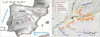

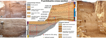

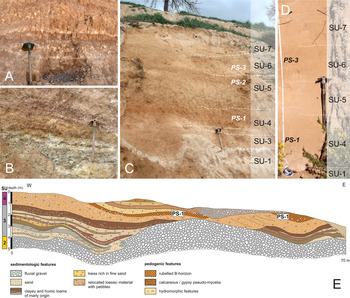


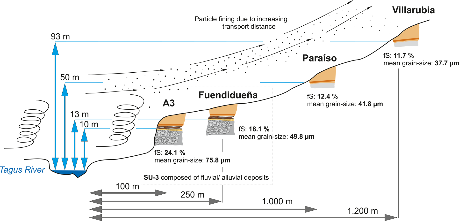


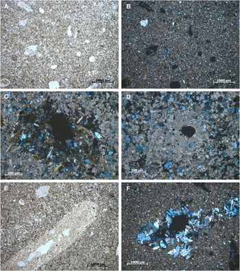


 Open access