Impact of Economic Freedom on Corruption Revisited in ASEAN Countries: A Bayesian Hierarchical Mixed-Effects Analysis


1
Institute for Research Science and Banking Technology, Banking University of Ho Chi Minh City, 39 Ham Nghi Street, District 1, Ho Chi Minh City 700000, Vietnam
2
Finance, Economics and Management Research Group, Ho Chi Minh City Open University, 97 Vo Van Tan Street, District 3, Ho Chi Minh City 700000, Vietnam
*
Author to whom correspondence should be addressed.
Economies 2021, 9(1), 3; https://doi.org/10.3390/economies9010003
Submission received: 14 August 2020
/
Revised: 1 December 2020
/
Accepted: 28 December 2020
/
Published: 5 January 2021
(This article belongs to the Special Issue Impact of Corruption on the Economy)
Abstract
:Conceptual and applied studies assessing the linkage between economic freedom and corruption expect that economic freedom boosts economic growth, improves income, and reduces levels of corruption. However, most of them have concentrated on developed and developing groups, while the Association of Southeast Asian Nations (ASEAN) countries have drawn much less attention. Empirical findings are most often conflicting. Moreover, previous studies performed rather simple frequentist techniques regressing one or some freedom indices on corruption that do not allow for grasping all the aspects of economic freedom as well as capturing variations across countries. The study aims to investigate the effects of ten components of economic freedom index on the level of corruption in ten ASEAN countries from 1999 to 2018. By applying a Bayesian hierarchical mixed-effects regression via a Monte Carlo technique combined with the Gibbs sampler, the obtained results suggest several findings as follows: (i) In view of probability, the predictors property rights, government integrity, tax burden, business freedom, labor freedom, and investment freedom have a strongly positive impact on the response perceived corruption index; (ii) Government spending, trade freedom, and financial freedom exert a strongly negative effect, while the influence of monetary freedom is ambiguous; and (iii) There is an existence of not only random intercepts but also random coefficients at the country level impacting the model outcome. The empirical outcome could be of major importance for more efficient corruption controlling in emerging countries, including ASEAN nations.
Keywords:
economic freedom; corruption; economic growth; Bayesian hierarchical mixed-effects regression; ASEAN countriesJEL Classiflcation Code:
C11; C33; D14; H31; H51; I131. Introduction
Economic growth is greatly dependent on institutions and institutional quality (North 1990). The prosperity of developed countries (e.g., OECD or the United States) is originated from their excellent institutional quality. Acemoglu et al. (2003) state that the institutional arrangement is a vital determinant of social and political development. High income, education, and infrastructure in developed countries are the dream of residents in poor or developing countries. However, changes in an institutional system take place slowly and difficultly (Dias and Tebaldi 2012; Glaeser et al. 2004). In addition, in developing countries, civil war and rampant corruption lead to depleting the beliefs of residents to their governments. So, Obstfeld (1994), Acemoglu and Zilibotti (1997) suggest that economic freedom and integration is a considerable solution for emerging countries.
According to Transparency International, “corruption as the abuse of entrusted power for private gain.” Many previous studies support that economic freedom reduces the level of corruption. The studies confirm this conclusion by Pieroni and d’Agostino (2013) and Graeff and Mehlkop (2003). Nevertheless, on the contrary, among the most corrupt countries, Billger and Goel (2009) discover that greater economic freedom does not reduce corruption and may even exacerbate it. Likewise, Godinez and Liu (2015) find that a higher level of corruption in host countries leads to more attracting foreign direct investment from multinational enterprises. These findings imply that the efficiency of corrupt controlling policies depends on the level of economic freedom and national development. Besides, Graeff and Mehlkop (2003) provide empirical evidence that greater economic freedom affects the likelihood of corruption in poor countries. However, this is not true for rich countries where corruption is better controlled by the legal structure and effectiveness of governments.
According to the report of the global public survey in 2013, about 50 percent of people in the Association of Southeast Asian Nations (ASEAN) countries believe corruption has increased, while only a third say their government’s efforts to fight corruption have been effective. In fact, many anti-corruption authorities in the ASEAN countries fall short of their full potential, often suffering from a lack of operational independence and limited capacities and resources. The report of Transparency International in 2014 shows that most ASEAN countries have medium or high levels of corruption, except for Malaysia and Singapore, while economic freedom tends to increase in these nations, hypothesizing an ambiguous relationship between economic freedom and corruption. This study investigates the impact of economic freedom on the level of corruption in the ASEAN countries during the period 1999–2018. However, our research differs from previous studies in the same field in several points, as follows:
First, the economic freedom index is built on twelve components, including property rights, judicial effectiveness, government integrity, tax burden, government spending, fiscal health, business freedom, labor freedom, money freedom, trade freedom, investment freedom, and financial freedom, while most previous studies used only the aggregate indicator of economic freedom or a few of its components (e.g., business freedom or money freedom) to analyze the influence of economic freedom on other macroeconomic variables, including corruption. These studies suggested several suitable policy implications but did not provide an insightful understanding of this problem because a few components could not stand for all characteristics of economic freedom (Berggren and Nilsson 2016). This work used all the components of the economic freedom index (except for judicial effectiveness and fiscal health index owing to missing data) to examine the influence of economic freedom on corruption (measured by the perceived corruption index), since not all areas affect corruption equally. Additionally, our focus is on the Government integrity indicator because differences in this dimension are a key determinant of anti-corrupt policies issued by governments. This implies that the success of anti-corrupt campaigns depends on the integrity of all political leaders and state officials.
Second, most previous studies were conducted in a simple linear framework, and suggested conclusions are based on frequentist techniques, where coefficient parameters are fixed estimates. More importantly, examining the links between all potential variables is impossible as non-significant coefficients are dropped out of analysis. In this work, we applied the Bayesian inference approach through the integrated Markov chain Monte Carlo sampler to provide probabilistic interpretations of model uncertainty and varying effects of ten components of economic freedom index on the corruption level in the ASEAN countries. The advantage of Bayesian inference as compared to frequentist inference is presented in Section 3. The empirical outcome by Bayesian inference of this study contributes to the existing literature, and for the ASEAN countries, in particular. Besides, the main advantage of the mixed-effects method is to capture differences from country to country, not only in initial corruption level but also in the other national features of government integrity.
The rest of the study is organized as follows: Section 2 focuses on the relevant literature and summarizes available studies. Section 3 presents the research model and methodology, while Section 4 shows the empirical results and discussion. The conclusion and policy implications are presented in Section 5.
2. Theoretical Background and Literature Review
2.1. Theoretical Background
The neoclassical growth theory suggests that the growth of a nation is dependent on four essential factors, including the capacity of raw material capital, physical capital accumulation, human capital accumulation, and technology. However, North (1990) and Acemoglu et al. (2003) explain that capital accumulation and technology are not the fundamental determinants of growth; in fact, they are growth themselves. They emphasize that development is originated from institutions. The difference in institutional quality is a key factor of national development in the long-term, which should generate a rich, medium-income, or poor country. Consistent with this view, Dias and Tebaldi (2012), Rose-Ackerman (2008), and Glaeser et al. (2004) argue that institutions contribute to shaping effective policies, more political stability, less violence, and boost economic growth. Economic freedom is a critical orientation, which influences every side of socio-economic life. So, economic freedom is tightly dependent on the view of the political leaders and the movements of society. In a country with institutional flexibility, all rights and legitimate interests of citizens are protected by national law. The majority of ideas or comments of residents are accepted by the administrators or officials (Davis 2010; Kacprzyk 2015; Krieger and Meierrieks 2016), and residents believe in existing policies issued by governments (Farhadi et al. 2015; Islam 1996, 2018; Shen and Williamson 2016). Unfortunately, this is not observed in the countries with civil war or weak government (Rose-Ackerman 2008).
Corruption is not a new phenomenon; its history predates the dawn of modern civilization (Mauro 1995). Corruption is defined as the abuse of entrusted power/position for private wealth. From the psychological perspective, seeking individual benefit is the primitive behavior of humans. According to the theory of cognitive appraisal proposed by Lazarus (1966), an individual will corrupt when he/she believes that his/her behavior will not be detected or sanctioned. In essence, corruption occurs where private gain and public power overlap. It represents that individuals and enterprises must pay illicit money to receive a public service or decision (e.g., license, certificate). So, corruption aggravates transaction costs for enterprises, stimulates dissatisfaction, and erodes the belief of residents in government. In this study, the level of corruption is measured by their perceived levels of public sector corruption. It uses a scale of zero to 100, where zero is highly corrupt, and 100 is very clean.
2.2. Literature Review
Many studies have analyzed the links between economic growth, corruption, and economic freedom in both developed and emerging countries, whose empirical results provided an insightful look into the economics of corruption. The pioneering study by Mauro (1995) shows that disorganized corruption reduces economic growth. Likewise, Rose-Ackerman (2008) confirms that corruption breeds inefficiencies and distortions of state policies, while Saha and Ben Ali (2017) conclude that corruption increases poverty and worsens income disparity. An alternative view, one of the reasons often cited for the existence of corruption, is that a bribe is simply a transfer and therefore entails no social severe welfare losses. Leff (2016) argues that corruption improves social welfare because it is a way to avoid cumbersome regulations, and it is a reward for badly paid bureaucrats. Even Rashid (1981) shows that corruption can “grease” an economic system and prevent it from reaching Pareto optimum.
Regarding the connection between economic freedom and corruption, Graeff and Mehlkop (2003) investigate the impact of various components of economic freedom on corruption. Using the corruption perception index as a proxy of corruption, the outcome obtained by the Ordinary Least Square (OLS) estimator shows that there is a strong relationship between economic freedom and corruption. However, this relation is different between poor countries and rich countries, which depends on the level of national development. Das and DiRienzo (2009) examine the hypothesis that globalization has increased the opportunity for anti-corrupt practice in 113 countries. The empirical results reveal that economic freedom has a positive impact on the corruption level (measured by the corruption perception index). Accordingly, a one-point increase in the economic freedom index leads to a 0.101 point increase in the corruption perception index, meaning that greater economic freedom reduces corruption behavior in the examined countries.
Likewise, Saha et al. (2009) discover the influence of economic freedom, democracy, and its interaction effect on controlling corruption in 100 countries from 1995 to 2004. The results of the fixed effect model indicate that both economic freedom and democracy significantly combat corruption. Indeed, the obtained estimation shows that economic freedom reduces corruption in any political environment, while democracy increases corruption when economic liberalization is low. A general conclusion that corruption negatively affects economic growth may not be convincing. Carden and Verdon (2010) suspect that the conventional thesis that corruption is always and everywhere a bad thing may not necessarily be true. They explore how different kinds of corruption interact with economic freedom to affect economic growth in 45 countries from 1995 to 2005. Accordingly, the outcome suggests that military corruption appears to have a robust negative effect on economic growth, while corruption in the education system tends to be positively correlated with economic growth. Economic freedom and business corruption independently increase GDP growth, but they work against each other. That means business corruption may “grease the wheels” of commerce in environments with relatively insecure contracting institutions.
“Live free or bribe: On the causal dynamics between economic freedom and corruption in U.S. states” is the title of a study by Apergis et al. (2012). They analyze the connection between economic freedom and corruption in the United States. Using annual data from all 50 U.S. states over the period 1981 to 2004 and applying the panel error correction model, the empirical results reveal that economic freedom has a negative and statistically significant impact on corruption in the long-run, while the causality test presents that there is bi-directional causality between economic freedom and corruption in both the short- and long-run. Another study by Saha and Su (2012) inspects the interaction effects of economic freedom and democracy in controlling corruption for 100 countries. The obtained estimation by the quantile regression technique provides empirical evidence on the interaction variable effect on reducing corruption, especially in the most corrupt countries.
Nevertheless, the influence of democratic and economic freedoms alone is ambiguous in the most-corrupt nations. Furthermore, a sound democratic reform can eliminate corruption substantially only after achieving a threshold level of economic freedom. Pieroni and d’Agostino (2013) analyze the impact of several components of economic freedom on corrupt practices for Africa and transition economy subsamples. The results show that the extent of the macro-effects on the measures of (micro) economic freedom for corruption is identified by the degree of economic development of a country. So, it re-confirms the conclusion by Graeff and Mehlkop (2003).
Recently, Shen and Williamson (2016) used structural equation modeling to examine the linkages between corruption, democracy, economic freedom, and state strength for 91 nations. Their analyses report four major findings: (i) Democracy (measured by political rights, civil liberties, and press freedom) has a positive influence; (ii) State strength has a positive direct effect; (iii) Economic freedom has a positive effect; and (iv) Ethnolinguistic fractionalization has both direct and indirect negative effects on the perceived corruption index. Of course, the above-mentioned studies do not adequately represent all of the existing previous studies on economic growth–corruption–economic freedom connection. However, this review shows that most previous studies are conducted in the linear framework, and their conclusions are based on frequentist inference, which is an obsolete estimator (Kalli and Griffin 2018; Kim 2002; Norets 2015). To the best of our knowledge, no previous studies used Bayesian inference to analyze the impact of all the components of the economic freedom index on the corrupt level in ten ASEAN countries. So, it is a research gapthat the study wants to address. The results acquired by Bayesian inference will enrich the existing literature on economic freedom and could be of major importance for more efficient corrupt control in emerging countries.
3. Research Model, Methodology, and Data
3.1. Research Model and Methodology
Mixed-effects regression models have been employed extensively in a diversity of fields, from the social sciences and health to econometrics. The terms “fixed” and “random” are being used in the statistics-biostatistics sense: A fixed coefficient is an unknown constant of nature, while a random coefficient is one that varies from a sample of groups to a sample of groups. The fixed effects similar to frequentist regression coefficients are estimated directly, while the estimation of the random effects is not direct but through their estimated variances and covariances. Random effects obtain two forms: random intercepts and random coefficients. Mixed-effects models use the grouping structure of the data, which may consist of multiple levels of nested groups. Also, mixed-effects models are well-known in econometrics literature as hierarchical models too. Fixed effects are, essentially, predictor variables. These are the effects we pay attention to after taking random variability into account (thus, fixed). Random effects are best considered as noise in our data as they arise from uncontrollable variability within a sample.
The current research applies a mixed-effects method within the Bayesian approach. To predict the values of a response variable, we can use a simple linear regression. However, as believing that there are differences between countries, we include this in the model, which incorporates both random intercepts and random coefficients. That is, not only intercepts but also slopes are different from country to country. Due to the rapid development of computer sciences and informative technology during the past decades, the Bayesian paradigm has been becoming a more and more widely used methodology (Nguyen et al. 2019a; Nguyen and Thach 2019; Nguyen et al. 2019b; Sriboonchitta et al. 2019; Svítek et al. 2019; Thach 2020a, 2020b; Thach et al. 2020). The Bayesian framework has many superiorities to more traditional frequentist inference. First of all, universality may be the greatest advantage of Bayesian methods, where Bayes’s rule, a simple law of probability, can be applied to all the parametric regressions. In contrast, a frequentist regression method constructed for a class of models is inappropriate for other classes. Frequentist and Bayesian inferences rely on distinct philosophies. Bayesian parameters are random, whereas frequentist parameters are unknown, but fixed. From this feature, Bayesian estimates are an entire probability distribution of a particular coefficient, while frequentist results are point estimates. Besides, combining prior distributions with observed data results in a more balanced, more accurate, and more valid Bayesian inference. More importantly, while data-driven frequentist methods face the effect of small sample size, but Bayesian methods do not. Unlike data-driven frequentist inference, the combination of data likelihood with prior distribution in Bayesian inference allows for overcoming the endogeneity problem attributed to the former method. Last, the Bayesian framework permits us to make probability statements, such as a relationship between parameters is likely or unlikely, or the prespecified probability of an interval containing the true value of a coefficient of interest.
The prior choice is problematic in Bayesian modeling owing to its subjectivity. That is, different researchers might make different prior choices for the same model. Priors are defined as pre-existing information about model parameters and are often derived from theoretical or empirical results or expert knowledge. Fortunately, however, there are underlying principles in prior choice. Firstly, prior distribution should not overwhelm data distribution in a case with a large sample. If our data sample is sufficiently large, then noninformative priors can be specified. Secondly, as we are faced with a small data sample, the employment of noninformative priors may cause Type I error or Type M error. So, it is recommended to apply weakly informative (Lemoine 2019). In our case, following Lemoine (2019), to obtain a balanced posterior regression model, we specify weakly informative priors. Accordingly, we perform simulations with normal prior distributions. A normal (0, 1) prior is assigned to model parameters in previous studies (Block et al. 2011; Thach 2020a, 2020b). As recommended by these authors, to check for model robustness, we can analyze the sensitivity of results to prior specification. We specify the target Markov chain Monte Carlo (MCMC) sample size of 3000 and the first 2500 iterations for the burn-in period discarded from the MCMC sample. The values of parameters simulated during burn-in are used for adaptation purposes only and are not used for estimation. To avoid high autocorrelation of the simulated MCMC sample in a high-dimensioned mixed model, we set a thinning of 500. So, the total number of iterations for the Metropolis-Hastings algorithm equals 1,502,001.
In the application of a Monte Carlo technique, chain convergence diagnostics should be performed before proceeding to inference. Once MCMC convergence is achieved, MCMC chains have converged to the desired distribution. Our general econometric model is specified as follows:
where PCI is the perceived corruption index introduced by Transparency International; X is ten indices of economic freedom introduced by The Heritage Foundation; β is a vector of coefficients; ui are random intercepts; ϑi is a random coefficient (slope) of the variable government integrity of interest; subscripts i, t, and p are country, year, and coefficient parameter, respectively. The CO is the control variable, including: human development index (HDI) and GDP per capita (at the fixed price 2010, unit: U.S. dollar).
3.2. Data Description
The perceived corruption index (PCI) and twelve components of the economic freedom index (EFI) are collected from Transparency International and the Heritage Foundation for ten ASEAN countries from 1999 to 2018. According to experts and business people, the PCI is measured by their perceived levels of public sector corruption. It uses a scale of zero to 100, where zero is highly corrupt, and 100 is very clean. The EFI is measured based on twelve quantitative and qualitative factors, grouped into four pillars, including: (1) Rule of Law (property rights (PR); government integrity (GI); judicial effectiveness, (JE)); (2) Government Size (government spending (GS); tax burden (TB); fiscal health (FH)); (3) Regulatory Efficiency (business freedom (BF); labor freedom (LF); monetary freedom (MF)); (4) Open Markets (trade freedom (TF); investment freedom (IF); financial freedom (FF)). Each of the twelve components is graded on a scale of zero to 100, where a higher point is more advanced in economic freedom. This work used ten components (except for judicial effectiveness (JE) and fiscal health (FH) index, due to the reason for missing data) to examine the influence of economic freedom on corruption. The HDI variable is collected from the United Nations Development Programmer (UNDP), while the GDP variable is collected from the World Bank. The descriptive statistic of all variables is presented in Table 1.
4. Empirical Results and Discussion
4.1. Posterior Simulations
As mentioned above, a great superiority of the Bayesian approach is that Bayesian methods provide intuitive and direct probabilistic interpretations of results that frequentist techniques cannot do. Bayesian results are an entire probability distribution of a particular coefficient. Also, we can state clearly what is a probability that the true value of a parameter of interest falls into a certain range.
The estimated probabilities, recorded in Table 2, demonstrate that the predictor variables PR, GI, TB, BF, LF, and IF have a strongly positive effect on the response PCI, while variables GS, TF, and FF strongly negatively contribute to the response PCI (with a range of probabilities from 0.73 to 1). It is noted that the impact of the predictor MF is ambiguous as the probability of the effect is only about 0.57. Importantly, as mentioned earlier, Bayesian methods allow one to capture the effects of all the parameters despite the weak impact of some certain variables, which might be ignored in standard frequentist statistics.
According to the results shown in Table 2, standard deviation values of the parameters are small, while MCMC errors (MCSE) are close to one decimal, which is, as usual, acceptable for Monte Carlo algorithms. These obtained results confirm the high accuracy of the parameter estimates.
Five estimated random intercepts and random coefficients (for variable Government integrity (GI) in our case) are chosen randomly and displayed in Table 3. The simulation results in this table prove that for these random intercepts and random coefficients, standard deviations are small, MCSE are also inconsiderable, that is, less than one decimal, which is acceptable for MCMC sampling. In general, the less MCSE, the more accurate the mean estimates of the effects. The similar estimates of mean and median show symmetric distributions. In sum, these results suggest that the outcome of our model is influenced not only by fixed effects but also by random effects.
4.2. Checks for Model Robustness
Owing to lack of data, frequentist methods suffer from the endogeneity problem. Fortunately, the Bayesian rule, a universal probability rule allows for a solution to this problem. To prove this advantage of the Bayesian paradigm, referring to Block et al. (2011), we vary the mean of normal prior in a range from −0.5 to 0.5 with an even space of 0.1. If point and interval estimates with regard to various priors for the parameters show no great differences, e.g., posteriors simulation results are not sensitive to prior choice, then our model is robust to endogeneity. Comparison results are presented in Appendix A, where no evident discrepancy is observed.
We are interested in the particular variable GI and consider its endogeneity. In our case, human capital (proxied by HDI) and GDP (proxied by GDP per capita) are suspected to be corrected with government integrity. We compare the outcome of IV regression with that of Bayesian regression. The results of IV regression show that the GI variable is really endogenous and HDI and GDP are its instruments; except for statistically non-significant PR, TB, BF, LF, MF, TF, FF variables resulting from IV regression, the coefficients of three remaining significant variables GI, GS, IF have the same sign as those obtained from Bayesian estimation (GI and IF variables positively affect PCI, while GS negatively impacts PCI). When extending the model by adding variables HDI and GDP as covariates, the overall variance of the extended model becomes smaller, the MCMC errors of three variables GI, GS, IF—smaller, that is, their estimates—more precise than those estimated in the initial model without variables HDI and GDP, that is, model uncertainty becomes less.
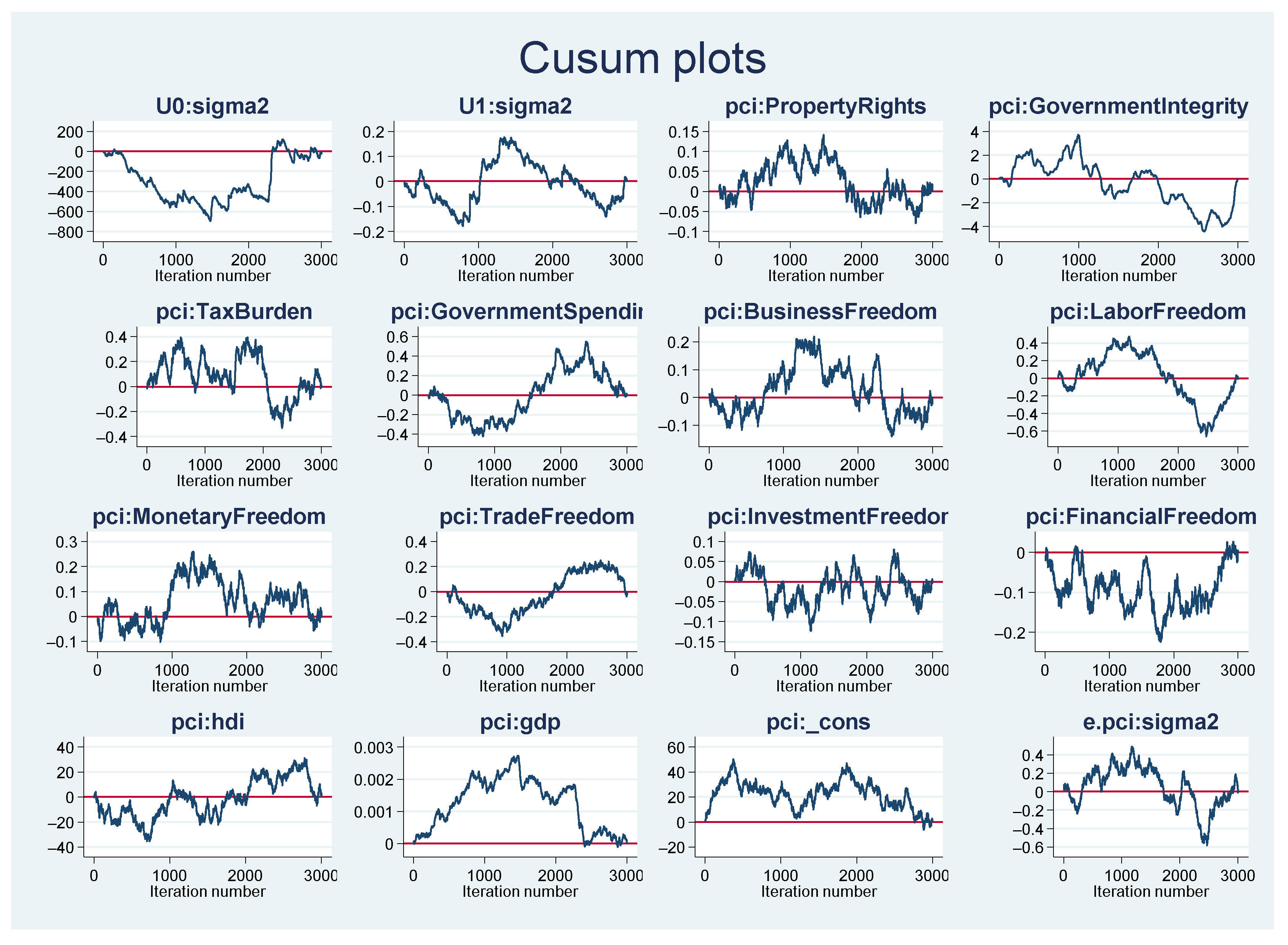
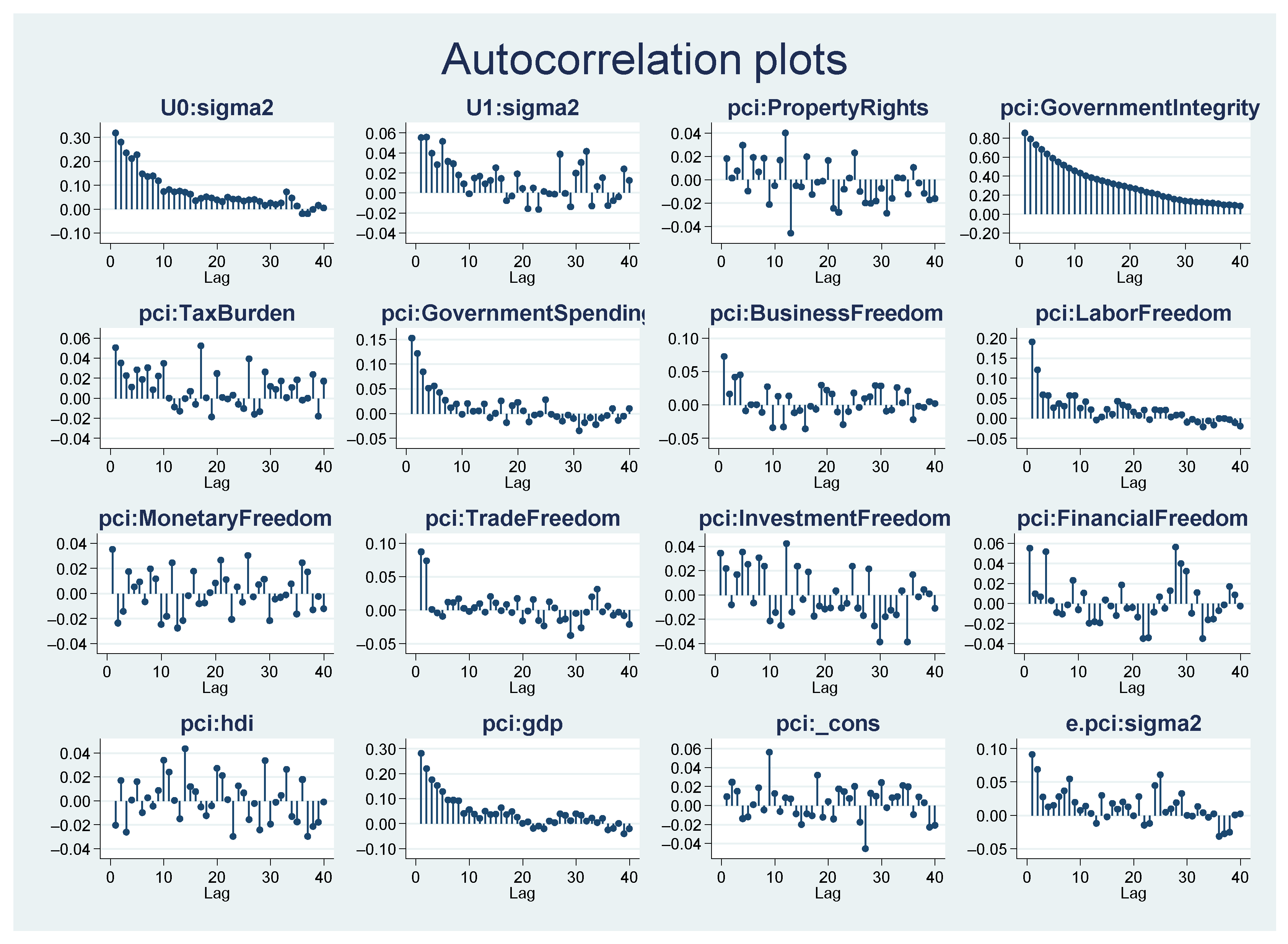
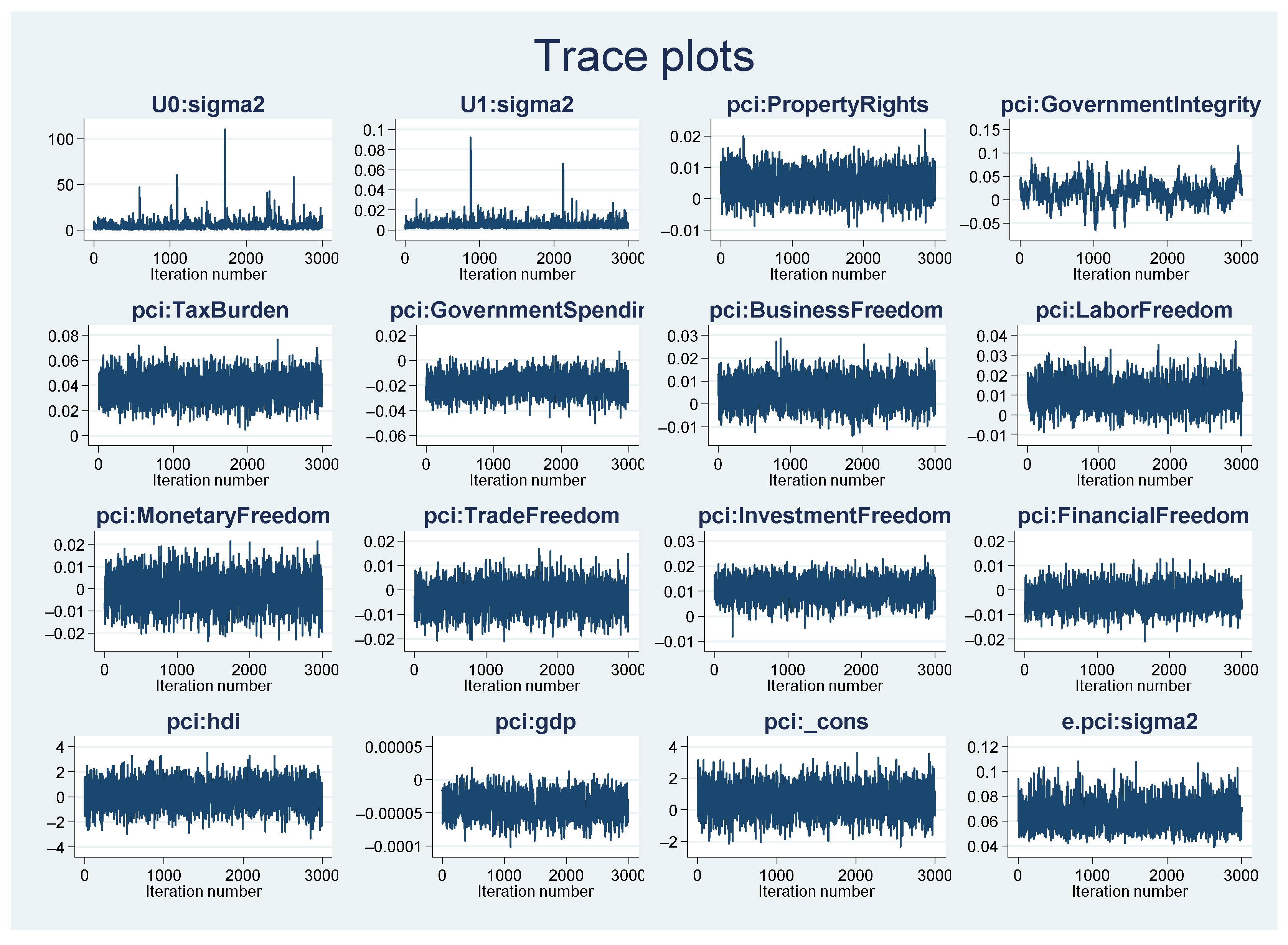
Besides, in applying MCMC algorithms, checks for chain convergence are needed. The estimation summary reports that initial efficiency indicators such as the rate of acceptance and average efficiency are large enough to have MCMC chains to acquire convergence. Concretely, for the model, where the parameters are assigned a (0, 1) normal prior, acceptance rate obtains a value of 0.57 (recommended indicator is 0.1), while average efficiency is equivalent to 0.65 (warning level is 0.01). The visual test shows a sign of good mixing of MCMC sequences when cusum plots are jagged, not smooth, crossing the X-axis. Cusum jagged lines for the parameters show no sign of non-convergence (see Figure 1). In addition to cusum plots, we can use trace and autocorrelation plots as popular tests for convergence check. The autocorrelation plots for all the parameters show that the plots die off after only few lags. Even that the autocorrelation plot for GI dies off after about 28 lags can be considered acceptable (Figure 2). These tests indicate no sign of non-convergence of MCMC chains. For all the model parameters, trace plots traverse rapidly through the posterior domain without exhibiting any trend (Figure 3).
Besides cusum, trace, and autocorrelation plots, we can practice a formal test like effective sample sizes (ESS). The result in Table 4 indicates that for all the parameters, efficiency is more than 0.01 and the largest correlation time (for parameter government integrity) is less than 29, which is acceptable for MCMC convergence.
In sum, we can conclude that our Bayesian model does not suffer from a serious endogeneity problem. As the Markov chains have converged to the stationary distribution, the parameters of our model to reasonable values. Hence, the Bayesian inference will be valid.
4.3. Discussion
Comparing our results with the findings of the previous studies, we are in line with Das and DiRienzo (2009), Saha et al. (2009), Shen and Williamson (2016), confirming a positive impact of property rights (PR), government integrity (GI), business freedom (BF), and investment freedom (IF) on corruption. Indeed, Borensztein et al. (1998), Kumari and Sharma (2017), and Ngoc and Hai (2019) agree that multinational enterprises are more concerned with the level of corruption, infrastructure, and the market scale when choosing the host country. So, “free” competition, government integrity, and efficient regulations would lead to the success of anti-corruption policies and enhance economic growth. Additionally, the ASEAN countries have mutual law consultation, which helps to stabilize and improve the legal system of each country and consistency of administrative procedures. Indonesia and Thailand have passed a freedom of information law, while other countries have ratified the United Nations Convention Against Corruption. Citizens, businesses, and civil society are supported to participate in the reduction of corruption across the region fully.
The obtained results of this study show a negative effect of GDP per capita, government spending, and financial freedom on corruption. The reasons for these results may be: (i) More government spending would open opportunities for private gains (Swaleheen et al. 2018); (ii) More financial freedom boosts economic growth, improves income (Abid et al. 2016; Akhmat et al. 2013; Nguyen et al. 2019c), which provides a “fertile land” for corruption; and (iii) Rose-Ackerman (2008) argues that corruption is not different from trade activities. Individuals or enterprises accept the purchase because they want to achieve their own goal faster than others, or they want to overcome the cumbersome regulations of the law. Even in many cases, this is an “insurance certificate” to avoid risks before unexpected changes from policies that may adversely impact on their business. Transparency International acknowledges that the ASEAN countries have taken a strong approach towards prosecution and punishment of corrupt individuals over the last few years. However, this was not sufficient to fight corruption effectively. According to the World Bank Bribery Index, 30 percent of business transactions concerning public services require informal payments and gifts, and more than 40 percent of companies are expected to give gifts to secure public contracts in the ASEAN region. These imply that the idea to create a regional body or an ASEAN Integrity Community to tackle corruption at the national and regional level is extremely necessary.
In the study, the effect of HDI on PCI is ambiguous. In fact, HDI is a general index, and the interest in human development is partly a response to the concerns raised about the influence of increasing corruption on income per capita. However, the number of the public administrators who have a corrupt opportunity is limited compared to the population. Hence, the ambiguous influence of human development on PCI could be understood (Akhter 2004). In addition, corrupt activities are also transforming, from cash receiving to exploit policy loopholes. As a result, it is a challenging to detect corruption (Dias and Tebaldi 2012; Swaleheen et al. 2018).
5. Conclusions and Policy Implication
Corruption continues to be a pressing issue around the world, contributing to growing inequality and an erosion of democracy and public trust in governments. There is a strong link between corruption and economic freedom that is important to acknowledge, especially within emerging economies like the ASEAN countries. Corruption is much more likely to flourish where democratic foundations are weak and, as we have seen in many countries, where undemocratic and populist politicians can use it to their advantage. By applying the Bayesian hierarchical mixed-effects regression via a Monte Carlo technique combined with Gibbs sampling, the research estimates the impact of ten indices of economic freedom on the perceived corruption index in ten ASEAN countries. The posterior model includes both random intercepts and random coefficients. Our focus is on predictor Government integrity because it is a key determinant of the success of anti-corrupt campaigns. As a result, in view of probability, the predictors property rights, government integrity, tax burden, business freedom, labor freedom, and investment freedom have a strongly positive impact on the response PCI, whereas variables government spending, trade freedom, and financial freedom exert a strongly negative effect on the dependent variable PCI. Importantly, the 57% probability of the effect indicates an ambiguous influence of the predictor monetary freedom. Two control variables, HDI and GDP, have conflicting effects on PCI. The effect of HDI is rather ambiguous, while GDP negatively contributes to PCI. The estimation results point out that variations of initial corruption level and differences in government integrity across the ASEAN countries are significant.
Based on the empirical results, some policy implications are suggested:
Firstly, the Governments in ten ASEAN countries should make public administration procedures transparent. The application of software or E-government will make procedures more clear and easy to be implemented, while also reducing overloading in the state agencies, saving travel expenses for people/businesses. Therefore, corruption does not have any opportunity to develop.
Secondly, governments should encourage the oversight of people and social-political organizations. The rich experience of many countries in the anti-corruption campaign shows a need to promote participation in social-economic processes of residents and social-political organizations. In fact, it is well recognized that the residents of developed countries have a positive view of anti-corruption than residents of emerging countries, including the ASEAN nations (Dias and Tebaldi 2012).
The main limitation of this research is that owing to the high dimensionality of full mixed-effects models, the Monte Carlo simulation is a very time-consuming and highly autocorrelated process. So, the research cannot incorporate in the model random coefficients for all the model parameters, and our focus is only on the predictor government integrity.
Author Contributions
Introduction, literature reviews, discussion, and policy implication, B.H.N.; methodology, empirical results, and conclusion, N.N.T. All authors have read and agreed to the published version of the manuscript.
Funding
The APC was funded by The Banking University HCMC and the Ho Chi Minh Open University.
Data Availability Statement
The data presented in this study are openly available at: https://www.heritage.org/index/explore, and: https://www.transparency.org/en/cpi.
Acknowledgments
We thank anonymous reviewers and Editor-in-chief for very useful comments and suggestions. All errors are ours.
Conflicts of Interest
The authors declare no conflict of interest.
Appendix A

Table A1.
Sensitivity analysis with respect to prior specification.
| Variable | Mean | Std. Dev. | MCSE | Median | [95% Cred. Interval] | ||
| −0.5 | Property Rights | 0.005 | 0.004 | 0.000 | 0.005 | −0.003 | 0.013 |
| Government Integrity | 0.021 | 0.016 | 0.006 | 0.020 | −0.007 | 0.054 | |
| Tax Burden | 0.042 | 0.010 | 0.000 | 0.041 | 0.021 | 0.062 | |
| Government Spending | −0.020 | 0.008 | 0.001 | −0.020 | −0.034 | −0.005 | |
| Business Freedom | 0.006 | 0.006 | 0.001 | 0.005 | −0.006 | 0.018 | |
| Labor Freedom | 0.012 | 0.007 | 0.001 | 0.012 | −0.000 | 0.026 | |
| Monetary Freedom | −0.001 | 0.007 | 0.000 | −0.001 | −0.015 | 0.013 | |
| Trade Freedom | −0.003 | 0.005 | 0.000 | −0.003 | −0.013 | 0.008 | |
| Investment Freedom | 0.011 | 0.004 | 0.000 | 0.011 | 0.003 | 0.019 | |
| Financial Freedom | −0.003 | 0.004 | 0.000 | −0.003 | −0.012 | 0.006 | |
| HDI | −0.280 | 0.933 | 0.039 | −0.307 | −2.094 | 1.571 | |
| GDP | −0.000 | 0.000 | 0.000 | −0.000 | −0.000 | −0.000 | |
| Mean | Std. Dev. | MCSE | Median | [95% Cred. Interval] | |||
| −0.4 | Property Rights | 0.004 | 0.004 | 0.000 | 0.004 | −0.003 | 0.013 |
| Government Integrity | 0.022 | 0.016 | 0.005 | 0.021 | −0.009 | 0.053 | |
| Tax Burden | 0.041 | 0.011 | 0.000 | 0.041 | 0.019 | 0.062 | |
| Government Spending | −0.020 | 0.008 | 0.001 | −0.020 | −0.036 | −0.005 | |
| Business Freedom | 0.007 | 0.006 | 0.001 | 0.007 | −0.005 | 0.019 | |
| Labor Freedom | 0.013 | 0.007 | 0.001 | 0.013 | −0.001 | 0.027 | |
| Monetary Freedom | −0.002 | 0.007 | 0.000 | −0.002 | −0.016 | 0.012 | |
| Trade Freedom | −0.003 | 0.006 | 0.000 | −0.002 | −0.014 | 0.009 | |
| Investment Freedom | 0.010 | 0.004 | 0.000 | 0.010 | 0.002 | 0.018 | |
| Financial Freedom | −0.003 | 0.004 | 0.000 | −0.003 | −0.012 | 0.006 | |
| HDI | −0.116 | 0.966 | 0.032 | −0.123 | −2.019 | 1.769 | |
| GDP | −0.000 | 0.000 | 0.000 | −0.000 | −0.000 | −0.000 | |
| Mean | Std. Dev. | MCSE | Median | [95% Cred. Interval] | |||
| −0.3 | Property Rights | 0.004 | 0.004 | 0.000 | 0.004 | −0.004 | 0.012 |
| Government Integrity | 0.002 | 0.015 | 0.004 | 0.003 | −0.031 | 0.028 | |
| Tax Burden | 0.040 | 0.010 | 0.000 | 0.040 | 0.020 | 0.061 | |
| Government Spending | −0.019 | 0.008 | 0.001 | −0.018 | −0.033 | −0.004 | |
| Business Freedom | 0.005 | 0.005 | 0.000 | 0.005 | −0.005 | 0.016 | |
| Labor Freedom | 0.010 | 0.007 | 0.001 | 0.010 | −0.003 | 0.023 | |
| Monetary Freedom | −0.001 | 0.007 | 0.000 | −0.001 | −0.015 | 0.012 | |
| Trade Freedom | −0.002 | 0.006 | 0.001 | −0.002 | −0.012 | 0.009 | |
| Investment Freedom | 0.011 | 0.004 | 0.000 | 0.011 | 0.002 | 0.019 | |
| Financial Freedom | −0.003 | 0.004 | 0.000 | −0.003 | −0.012 | 0.006 | |
| HDI | −0.106 | 0.960 | 0.038 | −0.089 | −1.957 | 1.813 | |
| GDP | −0.000 | 0.000 | 0.000 | −0.000 | −0.000 | −0.000 | |
| Mean | Std. Dev. | MCSE | Median | [95% Cred. Interval] | |||
| −0.2 | Property Rights | 0.004 | 0.004 | 0.000 | 0.004 | −0.004 | 0.012 |
| Government Integrity | 0.022 | 0.012 | 0.002 | 0.022 | −0.003 | 0.044 | |
| Tax Burden | 0.041 | 0.010 | 0.000 | 0.041 | 0.021 | 0.061 | |
| Government Spending | −0.019 | 0.007 | 0.001 | −0.020 | −0.034 | −0.005 | |
| Business Freedom | 0.006 | 0.005 | 0.001 | 0.005 | −0.005 | 0.017 | |
| Labor Freedom | 0.012 | 0.007 | 0.001 | 0.012 | −0.002 | 0.025 | |
| Monetary Freedom | −0.001 | 0.007 | 0.000 | −0.001 | −0.015 | 0.012 | |
| Trade Freedom | −0.003 | 0.006 | 0.001 | −0.003 | −0.014 | 0.008 | |
| Investment Freedom | 0.011 | 0.004 | 0.000 | 0.011 | 0.003 | 0.019 | |
| Financial Freedom | −0.003 | 0.004 | 0.000 | −0.003 | −0.011 | 0.006 | |
| HDI | −0.015 | 0.945 | 0.034 | −0.009 | −1.854 | 1.856 | |
| GDP | −0.000 | 0.000 | 0.000 | −0.000 | −0.000 | −0.000 | |
| Mean | Std. Dev. | MCSE | Median | [95% Cred. Interval] | |||
| −0.1 | Property Rights | 0.004 | 0.004 | 0.000 | 0.005 | −0.004 | 0.013 |
| Government Integrity | 0.020 | 0.016 | 0.004 | 0.020 | −0.015 | 0.048 | |
| Tax Burden | 0.039 | 0.011 | 0.001 | 0.039 | 0.018 | 0.060 | |
| Government Spending | −0.020 | 0.008 | 0.001 | −0.020 | −0.036 | −0.005 | |
| Business Freedom | 0.006 | 0.006 | 0.001 | 0.006 | −0.005 | 0.017 | |
| Labor Freedom | 0.012 | 0.007 | 0.001 | 0.012 | −0.002 | 0.026 | |
| Monetary Freedom | −0.002 | 0.007 | 0.000 | −0.002 | −0.016 | 0.013 | |
| Trade Freedom | −0.003 | 0.006 | 0.001 | −0.003 | −0.014 | 0.009 | |
| Investment Freedom | 0.011 | 0.004 | 0.000 | 0.011 | 0.002 | 0.018 | |
| Financial Freedom | −0.003 | 0.004 | 0.000 | −0.003 | −0.012 | 0.005 | |
| HDI | 0.077 | 0.964 | 0.030 | 0.067 | −1.780 | 1.984 | |
| GDP | −0.000 | 0.000 | 0.000 | −0.000 | −0.000 | −0.000 | |
| Mean | Std. Dev. | MCSE | Median | [95% Cred. Interval] | |||
| 0 | Property Rights | 0.004 | 0.004 | 0.000 | 0.004 | −0.004 | 0.012 |
| Government Integrity | 0.014 | 0.014 | 0.005 | 0.014 | −0.017 | 0.042 | |
| Tax Burden | 0.039 | 0.011 | 0.001 | 0.039 | 0.018 | 0.060 | |
| Government Spending | −0.019 | 0.008 | 0.001 | −0.019 | −0.036 | −0.004 | |
| Business Freedom | 0.005 | 0.005 | 0.000 | 0.005 | −0.005 | 0.016 | |
| Labor Freedom | 0.010 | 0.007 | 0.001 | 0.010 | −0.003 | 0.024 | |
| Monetary Freedom | −0.001 | 0.007 | 0.000 | −0.001 | −0.015 | 0.012 | |
| Trade Freedom | −0.003 | 0.006 | 0.001 | −0.003 | −0.014 | 0.008 | |
| Investment Freedom | 0.011 | 0.004 | 0.000 | 0.011 | 0.003 | 0.019 | |
| Financial Freedom | −0.003 | 0.004 | 0.000 | −0.003 | −0.012 | 0.005 | |
| HDI | 0.131 | 0.965 | 0.038 | 0.127 | −1.771 | 2.053 | |
| GDP | −0.000 | 0.000 | 0.000 | −0.000 | −0.000 | −0.000 | |
| Mean | Std. Dev. | MCSE | Median | [95% Cred. Interval] | |||
| 0.1 | Property Rights | 0.005 | 0.004 | 0.000 | 0.005 | −0.003 | 0.013 |
| Government Integrity | −0.003 | 0.018 | 0.006 | −0.002 | −0.041 | 0.027 | |
| Tax Burden | 0.037 | 0.010 | 0.000 | 0.037 | 0.016 | 0.058 | |
| Government Spending | −0.020 | 0.008 | 0.001 | −0.020 | −0.036 | −0.006 | |
| Business Freedom | 0.006 | 0.006 | 0.000 | 0.005 | −0.005 | 0.017 | |
| Labor Freedom | 0.010 | 0.007 | 0.001 | 0.010 | −0.003 | 0.023 | |
| Monetary Freedom | −0.002 | 0.007 | 0.000 | −0.002 | −0.016 | 0.012 | |
| Trade Freedom | −0.003 | 0.005 | 0.001 | −0.003 | −0.014 | 0.008 | |
| Investment Freedom | 0.010 | 0.004 | 0.000 | 0.010 | 0.002 | 0.019 | |
| Financial Freedom | −0.003 | 0.004 | 0.000 | −0.003 | −0.012 | 0.005 | |
| HDI | 0.313 | 0.962 | 0.032 | 0.322 | −1.553 | 2.197 | |
| GDP | −0.000 | 0.000 | 0.000 | −0.000 | −0.000 | −0.000 | |
| Mean | Std. Dev. | MCSE | Median | [95% Cred. Interval] | |||
| 0.2 | Property Rights | 0.005 | 0.004 | 0.000 | 0.005 | −0.003 | 0.013 |
| Government Integrity | 0.020 | 0.018 | 0.006 | 0.020 | −0.021 | 0.055 | |
| Tax Burden | 0.036 | 0.011 | 0.001 | 0.036 | 0.016 | 0.058 | |
| Government Spending | −0.020 | 0.007 | 0.001 | −0.020 | −0.035 | −0.006 | |
| Business Freedom | 0.006 | 0.006 | 0.001 | 0.006 | −0.005 | 0.017 | |
| Labor Freedom | 0.010 | 0.006 | 0.001 | 0.009 | −0.003 | 0.022 | |
| Monetary Freedom | −0.002 | 0.007 | 0.000 | −0.002 | −0.016 | 0.012 | |
| Trade Freedom | −0.003 | 0.005 | 0.000 | −0.003 | −0.014 | 0.007 | |
| Investment Freedom | 0.011 | 0.004 | 0.000 | 0.010 | 0.002 | 0.019 | |
| Financial Freedom | −0.003 | 0.004 | 0.000 | −0.003 | −0.012 | 0.005 | |
| HDI | 0.362 | 0.989 | 0.042 | 0.374 | −1.630 | 2.263 | |
| GDP | −0.000 | 0.000 | 0.000 | −0.000 | −0.000 | −0.000 | |
| Mean | Std. Dev. | MCSE | Median | [95% Cred. Interval] | |||
| 0.3 | Property Rights | 0.005 | 0.004 | 0.000 | 0.005 | −0.003 | 0.013 |
| Government Integrity | 0.021 | 0.014 | 0.004 | 0.019 | −0.004 | 0.052 | |
| Tax Burden | 0.035 | 0.011 | 0.000 | 0.035 | 0.015 | 0.057 | |
| Government Spending | −0.021 | 0.008 | 0.001 | −0.021 | −0.036 | −0.006 | |
| Business Freedom | 0.005 | 0.005 | 0.000 | 0.005 | −0.006 | 0.015 | |
| Labor Freedom | 0.009 | 0.006 | 0.001 | 0.009 | −0.003 | 0.021 | |
| Monetary Freedom | −0.002 | 0.007 | 0.000 | −0.002 | −0.015 | 0.012 | |
| Trade Freedom | −0.004 | 0.005 | 0.000 | −0.004 | −0.015 | 0.007 | |
| Investment Freedom | 0.011 | 0.004 | 0.000 | 0.011 | 0.003 | 0.019 | |
| Financial Freedom | −0.003 | 0.004 | 0.000 | −0.003 | −0.012 | 0.005 | |
| HDI | 0.436 | 0.973 | 0.037 | 0.418 | −1.483 | 2.410 | |
| GDP | −0.000 | 0.000 | 0.000 | −0.000 | −0.000 | −0.000 | |
| Mean | Std. Dev. | MCSE | Median | [95% Cred. Interval] | |||
| 0.4 | Property Rights | 0.004 | 0.004 | 0.000 | 0.005 | −0.004 | 0.012 |
| Government Integrity | 0.006 | 0.019 | 0.008 | 0.005 | −0.032 | 0.042 | |
| Tax Burden | 0.035 | 0.010 | 0.000 | 0.035 | 0.015 | 0.055 | |
| Government Spending | −0.021 | 0.008 | 0.001 | −0.021 | −0.037 | −0.007 | |
| Business Freedom | 0.005 | 0.005 | 0.001 | 0.005 | −0.005 | 0.016 | |
| Labor Freedom | 0.010 | 0.007 | 0.001 | 0.010 | −0.003 | 0.024 | |
| Monetary Freedom | −0.002 | 0.007 | 0.000 | −0.002 | −0.015 | 0.012 | |
| Trade Freedom | −0.004 | 0.006 | 0.000 | −0.004 | −0.015 | 0.006 | |
| Investment Freedom | 0.010 | 0.004 | 0.000 | 0.010 | 0.002 | 0.019 | |
| Financial Freedom | −0.003 | 0.004 | 0.000 | −0.003 | −0.011 | 0.005 | |
| HDI | 0.511 | 0.951 | 0.034 | 0.525 | −1.379 | 2.398 | |
| GDP | −0.000 | 0.000 | 0.000 | −0.000 | −0.000 | −0.000 | |
| Mean | Std. Dev. | MCSE | Median | [95% Cred. Interval] | |||
| 0.5 | Property Rights | 0.004 | 0.004 | 0.000 | 0.004 | −0.004 | 0.013 |
| Government Integrity | −0.003 | 0.023 | 0.007 | −0.002 | −0.043 | 0.047 | |
| Tax Burden | 0.035 | 0.011 | 0.001 | 0.035 | 0.013 | 0.055 | |
| Government Spending | −0.020 | 0.008 | 0.001 | −0.020 | −0.036 | −0.005 | |
| Business Freedom | 0.005 | 0.005 | 0.000 | 0.005 | −0.005 | 0.016 | |
| Labor Freedom | 0.009 | 0.007 | 0.001 | 0.009 | −0.005 | 0.022 | |
| Monetary Freedom | −0.002 | 0.007 | 0.000 | −0.002 | −0.016 | 0.012 | |
| Trade Freedom | −0.004 | 0.006 | 0.001 | −0.004 | −0.015 | 0.007 | |
| Investment Freedom | 0.010 | 0.004 | 0.000 | 0.010 | 0.002 | 0.018 | |
| Financial Freedom | −0.004 | 0.004 | 0.000 | −0.004 | −0.012 | 0.005 | |
| HDI | 0.553 | 0.970 | 0.035 | 0.561 | −1.362 | 2.450 | |
| GDP | −0.000 | 0.000 | 0.000 | −0.000 | −0.000 | −0.000 | |
References
- Abid, Fathi, Slah Bahloul, and Mourad Mroua. 2016. Financial development and economic growth in MENA countries. Journal of Policy Modeling 38: 1099–117. [Google Scholar] [CrossRef]
- Acemoglu, Daron, and Fabrizio Zilibotti. 1997. Was Prometheus Unbound by Chance? Risk, Diversification, and Growth. Journal of Political Economy 105: 709–51. [Google Scholar] [CrossRef] [Green Version]
- Acemoglu, Daron, Simon Johnson, James Robinson, and Yunyong Thaicharoen. 2003. Institutional causes, macroeconomic symptoms: Volatility, crises and growth. Journal of Monetary Economics 50: 49–123. [Google Scholar] [CrossRef] [Green Version]
- Akhmat, Ghulam, Khalid Zaman, and Tan Shukui. 2013. Impact of financial development on SAARC’S human development. Quality & Quantity 48: 2801–16. [Google Scholar]
- Akhter, Syed H. 2004. Is globalization what it’s cracked up to be? Economic freedom, corruption, and human development. Journal of World Business 39: 283–95. [Google Scholar] [CrossRef] [Green Version]
- Apergis, Nicholas, Oguzhan C. Dincer, and James E. Payne. 2012. Live free or bribe: On the causal dynamics between economic freedom and corruption in U.S. States. European Journal of Political Economy 28: 215–26. [Google Scholar] [CrossRef]
- Berggren, Niclas, and Therese Nilsson. 2016. Tolerance in the United States: Does economic freedom transform racial, religious, political and sexual attitudes? European Journal of Political Economy 45: 53–70. [Google Scholar] [CrossRef] [Green Version]
- Billger, Sherrilyn M., and Rajeev K. Goel. 2009. Do existing corruption levels matter in controlling corruption? Journal of Development Economics 90: 299–305. [Google Scholar] [CrossRef]
- Block, Joern H., Peter Jaskiewicz, and Danny Miller. 2011. Ownership versus management effects on performance in family and founder companies: A Bayesian reconciliation. Journal of Family Business Strategy 2: 232–45. [Google Scholar] [CrossRef] [Green Version]
- Borensztein, Eduardo, Jose De Gregorio, and Jong-Wha Lee. 1998. How does foreign direct investment affect economic growth? Journal of International Economics 45: 115–35. [Google Scholar] [CrossRef] [Green Version]
- Carden, Art, and Lisa Verdon. 2010. When Is Corruption a Substitute for Economic Freedom? The Law and Development Review 3: 35–70. [Google Scholar] [CrossRef]
- Das, Jayoti, and Cassandra DiRienzo. 2009. The Nonlinear Impact of Globalization on Corruption. The International Journal of Business and Finance Research 3: 33–46. [Google Scholar]
- Davis, Lewis S. 2010. Institutional flexibility and economic growth. Journal of Comparative Economics 38: 306–20. [Google Scholar] [CrossRef]
- Dias, Joilson, and Edinaldo Tebaldi. 2012. Institutions, human capital, and growth: The institutional mechanism. Structural Change and Economic Dynamics 23: 300–12. [Google Scholar] [CrossRef]
- Farhadi, Minoo, Md Rabiul Islam, and Solmaz Moslehi. 2015. Economic Freedom and Productivity Growth in Resource-rich Economies. World Development 72: 109–26. [Google Scholar] [CrossRef]
- Glaeser, Edward L., Rafael La Porta, Florencio Lopez-de-Silanes, and Andrei Shleifer. 2004. Do Institutions Cause Growth? Journal of Economic Growth 9: 271–303. [Google Scholar] [CrossRef]
- Godinez, Jose R., and Ling Liu. 2015. Corruption distance and FDI flows into Latin America. International Business Review 24: 33–42. [Google Scholar] [CrossRef] [Green Version]
- Graeff, Peter, and Guido Mehlkop. 2003. The impact of economic freedom on corruption: Different patterns for rich and poor countries. European Journal of Political Economy 19: 605–20. [Google Scholar] [CrossRef]
- Islam, Sadequl. 1996. Economic freedom, per capita income and economic growth. Applied Economics Letters 3: 595–97. [Google Scholar] [CrossRef]
- Islam, Md Rabiul. 2018. Wealth inequality, democracy and economic freedom. Journal of Comparative Economics 46: 920–35. [Google Scholar] [CrossRef]
- Kacprzyk, Andrzej. 2015. Economic freedom–growth nexus in European Union countries. Applied Economics Letters 23: 494–97. [Google Scholar] [CrossRef]
- Kalli, Maria, and Jim E. Griffin. 2018. Bayesian nonparametric vector autoregressive models. Journal of Econometrics 203: 267–82. [Google Scholar] [CrossRef]
- Kim, Jae-Young. 2002. Limited information likelihood and Bayesian analysis. Journal of Econometrics 107: 175–93. [Google Scholar] [CrossRef]
- Krieger, Tim, and Daniel Meierrieks. 2016. Political capitalism: The interaction between income inequality, economic freedom and democracy. European Journal of Political Economy 45: 115–32. [Google Scholar] [CrossRef] [Green Version]
- Kumari, Reenu, and Anil Kumar Sharma. 2017. Determinants of foreign direct investment in developing countries: A panel data study. International Journal of Emerging Markets 12: 658–82. [Google Scholar] [CrossRef]
- Lazarus, Richard S. 1966. Psychological Stress and the Coping Process. New York: McGraw-Hill. [Google Scholar]
- Leff, Nathaniel H. 2016. Economic Development Through Bureaucratic Corruption. American Behavioral Scientist 8: 8–14. [Google Scholar] [CrossRef]
- Lemoine, Nathan P. 2019. Moving beyond noninformative priors: Why and how to choose weakly informative priors in Bayesian analyses. Oikos 128: 912–28. [Google Scholar] [CrossRef] [Green Version]
- Mauro, Paolo. 1995. Corruption and Growth. The Quarterly Journal of Economics 110: 681–712. [Google Scholar] [CrossRef]
- North, Douglass C. 1990. Institutions, Institutional Change, and Economic Performance. New York: Cambridge University Press. [Google Scholar]
- Ngoc, Bui Hoang, and Dang Bac Hai. 2019. The Impact of Foreign Direct Investment on Structural Economic in Vietnam. In Beyond Traditional Probabilistic methods in Econometrics, Paper presented at ECONVN 2019, Studies in Computational Intelligence, Ho Chi Minh City, Vietnam, January 14–16. Edited by Kreinovich Vladik, Thach Nguyen Ngoc, Trung Nguyen Duc and Van Thanh D. Cham: Springer, vol. 809, pp. 352–62. [Google Scholar]
- Nguyen, Hung T., and Nguyen Ngoc Thach. 2019. A Closer Look at the Modeling of Economics Data. In Beyond Traditional Probabilistic Methods in Econometrics. Paper presented at ECONVN 2019, Studies in Computational Intelligence, Ho Chi Minh City, Vietnam, January 14–16. Cham: Springer, pp. 100–12. [Google Scholar]
- Nguyen, Hung T., Songsak Sriboonchitta, and Nguyen Ngoc Thach. 2019a. On Quantum Probability Calculus for Modeling Economic Decisions. In Structural Changes and Their Econometric Modeling, Paper presented at International Conference of the Thailand Econometrics Society, Chiang Mai, Thailand, January 9–11. Cham: Springer, pp. 18–34. [Google Scholar]
- Nguyen, Hung T., Nguyen Duc Trung, and Nguyen Ngoc Thach. 2019b. Beyond Traditional Probabilistic Methods in Econometrics. In Paper presented at ECONVN 2019, Studies in Computational Intelligence, Ho Chi Minh City, Vietnam, January 14–16. Cham: Springer, pp. 3–21. [Google Scholar]
- Nguyen, Ha Minh, Ngoc Hoang Bui, and Duc Hong Vo. 2019c. The Nexus between Economic Integration and Growth: Application to Vietnam. Annals of Financial Economics 14: 1950014. [Google Scholar] [CrossRef]
- Norets, Andriy. 2015. Bayesian regression with nonparametric heteroskedasticity. Journal of Econometrics 185: 409–19. [Google Scholar] [CrossRef]
- Obstfeld, Maurice. 1994. Risk-taking, global diversification, and growth. The American Economic Review 84: 1310–29. [Google Scholar]
- Pieroni, Luca, and Giorgio d’Agostino. 2013. Corruption and the effects of economic freedom. European Journal of Political Economy 29: 54–72. [Google Scholar] [CrossRef] [Green Version]
- Rashid, Salim. 1981. Public Utilities in Egalitarian LDC’s: The Role of Bribery in Achieving Pareto Efficiency. Kyklos 34: 448–60. [Google Scholar]
- Rose-Ackerman, Susan. 2008. Corruption and Government. International Peacekeeping 15: 328–43. [Google Scholar] [CrossRef] [Green Version]
- Saha, Shrabani, and Mohamed Sami Ben Ali. 2017. Corruption and Economic Development: New Evidence from the Middle Eastern and North African Countries. Economic Analysis and Policy 54: 83–95. [Google Scholar] [CrossRef]
- Saha, Shrabani, and Jen-Je Su. 2012. Investigating the Interaction Effect of Democracy and Economic Freedom on Corruption: A Cross-Country Quantile Regression Analysis. Economic Analysis and Policy 42: 389–96. [Google Scholar] [CrossRef] [Green Version]
- Saha, Shrabani, Rukmani Gounder, and Jen-Je Su. 2009. The interaction effect of economic freedom and democracy on corruption: A panel cross-country analysis. Economics Letters 105: 173–76. [Google Scholar] [CrossRef] [Green Version]
- Shen, Ce, and John B. Williamson. 2016. Corruption, Democracy, Economic Freedom, and State Strength. International Journal of Comparative Sociology 46: 327–45. [Google Scholar] [CrossRef]
- Sriboonchitta, Songsak, Hung T. Nguyen, Olga Kosheleva, Vladik Kreinovich, and Thach Ngoc Nguyen. 2019. Quantum Approach Explains the Need for Expert Knowledge: On the Example of Econometrics. In Structural Changes and Their Econometric Modeling, Studies in Computational Intelligence, Paper presented at International Conference of the Thailand Econometrics Society Chiang Mai, Thailand, January 9–11. Cham: Springer, pp. 191–99. [Google Scholar]
- Svítek, Miroslav, Olga Kosheleva, Vladik Kreinovich, and Thach Ngoc Nguyen. 2019. Why Quantum (Wave Probability) Models Are a Good Description of Many Non-quantum Complex Systems, and How to Go Beyond Quantum Models. In Beyond Traditional Probabilistic Methods in Economics, Studies in Computational Intelligence, Paper presented at International Econometric Conference of Vietnam, Ho Chi Minh City, Vietnam, January 14–16. Cham: Springer, pp. 168–75. [Google Scholar]
- Swaleheen, Mushfiq, Mohamed Sami Ben Ali, and Akram Temimi. 2018. Corruption and public spending on education and health. Applied Economics Letters 26: 321–25. [Google Scholar] [CrossRef]
- Thach, Nguyen Ngoc. 2020a. How to Explain When the ES Is Lower Than One? A Bayesian Nonlinear Mixed-Effects Approach. Journal of Risk and Financial Management 13: 21. [Google Scholar] [CrossRef] [Green Version]
- Thach, Nguyen Ngoc. 2020b. The Variable Elasticity of Substitution Function and Endogenous Growth: An Empirical Evidence from Vietnam. International Journal of Economics and Business Administration VIII: 263–77. [Google Scholar]
- Thach, Nguyen Ngoc, Kreinovich Vladik, and Trung Nguyen Duc. 2020. Data Science for Financial Econometrics. In Proceedings of the ECONVN 2020, Studies in Computational Intelligence, Ho Chi Minh City, Vietnam, January 14–16. Cham: Springer. [Google Scholar]
Figure 1.
Convergence test via cusum plots. Source: the author’s calculations.

Figure 2.
Convergence test via autocorrelation plots. Source: the author’s calculations.

Figure 3.
Convergence test via trace plots. Source: the author’s calculations.

Table 1.
Descriptive Statistics.
| Variable | Obs | Mean | Std. Dev. | Min | Max |
|---|---|---|---|---|---|
| Perceived corruption index (PCI) | 177 | 3.884 | 2.183 | 1.3 | 9.4 |
| Property Rights | 165 | 41.753 | 24.883 | 10 | 98.4 |
| Government Integrity | 165 | 37.725 | 22.643 | 10 | 94 |
| Tax Burden | 165 | 80.428 | 8.884 | 32.5 | 91.6 |
| Government Spending | 165 | 85.739 | 7.525 | 57.3 | 95.4 |
| Business Freedom | 165 | 63.305 | 17.973 | 29.2 | 100 |
| Labor Freedom | 117 | 66.042 | 15.854 | 43.6 | 98.9 |
| Monetary Freedom | 165 | 75.673 | 10.105 | 13.8 | 93 |
| Trade Freedom | 165 | 72.806 | 10.509 | 47.6 | 90 |
| Investment Freedom | 165 | 46.303 | 19.992 | 10 | 90 |
| Financial Freedom | 165 | 45.636 | 16.939 | 10 | 80 |
| Human Development index (HDI) | 200 | 0.664 | 0.132 | 0.402 | 0.932 |
| GDP | 200 | 10,184.723 | 15,361.787 | 269.291 | 58,691.915 |
Table 2.
Posterior simulation results of the model.
| Variables | Mean | Std. Dev. | MCMC Errors | Prob of Mean > 0 | [95% Cred. Interval] |
|---|---|---|---|---|---|
| Dependent Variable: PCI | |||||
| Property Rights | 0.00451 | 0.00405 | 0.00007 | 0.871 | [−0.0035, 0.0127] |
| Government Integrity | 0.01776 | 0.02291 | 0.00222 | 0.807 | [−0.0285, 0.0633] |
| Tax Burden | 0.0383 | 0.01017 | 0.00022 | 1 | [0.0186, 0.0583] |
| Government Spending | −0.01952 | 0.00777 | 0.00021 | 0.994 * | [−0.0349, −0.0045] |
| Business Freedom | 0.00517 | 0.00567 | 0.00012 | 0.815 | [−0.0051, 0.0164] |
| Labor Freedom | 0.01044 | 0.00655 | 0.00019 | 0.951 | [−0.0023, 0.0236] |
| Monetary Freedom | −0.00124 | 0.00704 | 0.00013 | 0.574 * | [−0.0152, 0.0128] |
| Trade Freedom | −0.00327 | 0.00539 | 0.00011 | 0.729 * | [−0.0139, 0.0072] |
| Investment Freedom | 0.01062 | 0.00407 | 0.00008 | 0.993 | [0.0024, 0.0184] |
| Financial Freedom | −0.00305 | 0.00441 | 0.00009 | 0.758 * | [−0.0115, 0.0059] |
| HDI | 0.18100 | 0.96137 | 0.01703 | 0.576 | [−1.7351, 2.0754] |
| GDP | −0.00004 | 0.00002 | 0.0000 | 0.989 * | [−0.0001, -0.0000 |
| Intercept | 0.61360 | 0.87669 | 0.01601 | 0.762 | [−1.0985, 2.3562] |
| U0: sigma2 U1: sigma2 | 4.00026 0.00473 | 4.61210 0.00359 | 0.22154 0.00008 | [0.3776, 14.133] [0.0016, 0.0129] | |
| e.pci | |||||
| sigma2 | 0.06516 | 0.01039 | 0.00025 | [0.0479, 0.0886] | |
Note: * is probability of mean coefficient < 0.
Table 3.
Posterior summaries of representative random intercepts and random coefficients.
| U0[id] | Mean | Std. Dev. | MCMC Errors | Median | [95% Cred. Interval] |
| 1 | 2.6184 | 1.1414 | 0.0523 | 2.5835 | [0.5129, 4.9543] |
| 2 | −1.2997 | 0.8260 | 0.0416 | −1.2414 | [−3.0115, 0.2338] |
| 3 | −1.1378 | 0.7125 | 0.0378 | −1.0973 | [−2.6971, 0.1217] |
| 4 | −0.0666 | 0.6897 | 0.0376 | −0.0207 | [−1.5187, 1.2044] |
| 5 | 1.4085 | 1.0738 | 0.0551 | 1.3528 | [−0.5536, 3.6079] |
| U1[id] | Mean | Std. Dev. | MCMC Errors | Median | [95% Cred. Interval] |
| 1 | −0.0168 | 0.0263 | 0.0021 | −0.0167 | [−0.0687, 0.0345] |
| 2 | −0.0188 | 0.0272 | 0.0022 | −0.0193 | [−0.0739, 0.0356] |
| 3 | 0.0307 | 0.0246 | 0.0022 | 0.0308 | [−0.0175, 0.0797] |
| 4 | −0.0372 | 0.0246 | 0.0022 | −0.0367 | [−0.0856, 0.0138] |
| 5 | −0.0185 | 0.0275 | 0.0023 | −0.0178 | [−0.0737, 0.0374] |
Table 4.
Convergence test via effective sample size.
| Effective Sample Sizes ESS | Corr. Time | Efficiency | |
|---|---|---|---|
| PCI | |||
| Property Rights | 2894.64 | 1.04 | 0.9649 |
| Government Integrity | 106.69 | 28.12 | 0.0356 |
| Tax Burden | 2149.65 | 1.40 | 0.7166 |
| Government Spending | 1407.27 | 2.13 | 0.4691 |
| Business Freedom | 2218.78 | 1.35 | 0.7396 |
| Labor Freedom | 1226.73 | 2.45 | 0.4089 |
| Monetary Freedom | 2913.27 | 1.03 | 0.9711 |
| Trade Freedom | 2268.17 | 1.32 | 0.7561 |
| Investment Freedom | 2697.17 | 1.11 | 0.8991 |
| Financial Freedom | 2702.22 | 1.11 | 0.9007 |
| HDI | 3000.00 | 1.00 | 1.0000 |
| GDP | 683.39 | 4.39 | 0.2278 |
| _Intercept | 3000.00 | 1.00 | 1.0000 |
| id | |||
| U0:sigma2 | 433.41 | 6.92 | 0.1445 |
| U1:sigma2 | 1852.76 | 1.62 | 0.6176 |
| e.pci | |||
| sigma2 | 1753.46 | 1.71 | 0.5845 |
Source: the author’s calculations.
Publisher’s Note: MDPI stays neutral with regard to jurisdictional claims in published maps and institutional affiliations. |
© 2021 by the authors. Licensee MDPI, Basel, Switzerland. This article is an open access article distributed under the terms and conditions of the Creative Commons Attribution (CC BY) license (http://creativecommons.org/licenses/by/4.0/).
Share and Cite
MDPI and ACS Style
Thach, N.N.; Ngoc, B.H. Impact of Economic Freedom on Corruption Revisited in ASEAN Countries: A Bayesian Hierarchical Mixed-Effects Analysis. Economies 2021, 9, 3. https://doi.org/10.3390/economies9010003
AMA Style
Thach NN, Ngoc BH. Impact of Economic Freedom on Corruption Revisited in ASEAN Countries: A Bayesian Hierarchical Mixed-Effects Analysis. Economies. 2021; 9(1):3. https://doi.org/10.3390/economies9010003
Chicago/Turabian StyleThach, Nguyen Ngoc, and Bui Hoang Ngoc. 2021. "Impact of Economic Freedom on Corruption Revisited in ASEAN Countries: A Bayesian Hierarchical Mixed-Effects Analysis" Economies 9, no. 1: 3. https://doi.org/10.3390/economies9010003
Note that from the first issue of 2016, this journal uses article numbers instead of page numbers. See further details here.