Searching for a Theory That Fits the Data: A Personal Research Odyssey

Department of Economics, University of Copenhagen, DK-1353 Copenhagen, Denmark
Econometrics 2021, 9(1), 5; https://doi.org/10.3390/econometrics9010005
Submission received: 6 July 2018
/
Revised: 2 January 2021
/
Accepted: 11 January 2021
/
Published: 1 February 2021
(This article belongs to the Special Issue Celebrated Econometricians: Katarina Juselius and Søren Johansen)
Abstract
:This survey paper discusses the Cointegrated Vector AutoRegressive (CVAR) methodology and how it has evolved over the past 30 years. It describes major steps in the econometric development, discusses problems to be solved when confronting theory with the data, and, as a solution, proposes a so-called theory-consistent CVAR scenario. A number of early CVAR applications are motivated by the urge to find out why the empirical results did not support Milton Friedman’s concept of monetary inflation. The paper also proposes a method for combining partial CVAR analyses into a large-scale macroeconomic model. It argues that an empirically-based approach to macroeconomics preferably should be based on Keynesian disequilibrium economics, where imperfect knowledge expectations replace so called rational expectations and where the financial sector plays a key role for understanding the long persistent movements in the data. Finally, the paper argues that the CVAR is potentially a candidate for Haavelmo’s “design of experiment for passive observations” and provides several illustrations.
Keywords:
cointegrated VAR; methodology; linking theory to evidence; empirically-based macroeconomicsJEL Classification:
B41; C32; C51; C521. Introduction
I was happy to accept the invitation by the guest editors to write this survey paper based on my retirement lecture given at the Economics Department of the University of Copenhagen in 2014. Retirement is one of the important dividing lines in a long active life that gives you the opportunity to slow down and to reflect on your achievements. When preparing for my retirement lecture I asked myself: who inspired me to choose econometrics; what were the main questions that motivated my research; how did I go about answering them; what stones did I stumbled on; and the most important one: did my research contribute to useful answers of important questions. In writing this paper, I have allowed myself to focus almost exclusively on my own research together with my many coauthors. While the paper is far from a balanced account of all the good research that has inspired me, the bibliographies in the papers to be discussed bear witness of the many important contributions on which this research rests.
Over a long academic career it is almost unavoidable that some scholars have been more influential than others. For me, David Hendry and Clive Granger were enormously influential for my thinking in the early formative years. I found the “general-to-specific” error correction approach developed by David utterly exciting and the numerous time-series methods proposed by Clive very inspiring. To be a colleague and a friend of both of them has been an invaluable privilege in all these years.1 My research has benefitted a lot from their highly innovative research.
However, it was the working paper on cointegration and error correction (Granger 1983) that fundamentally changed both my professional career and my personal life. From the outset I was intrigued by the concept of cointegration and how it related to the more familiar concept of error-correction. Clive’s paper defined cointegration as part of a vector moving average model for unobservable errors, whereas error correction models were based on the autoregressive model formulated for variables. At that time it was difficult to estimate moving average models—definitely more so than error correction models—and I could not see how to use cointegration in empirical work. Therefore, I asked Søren Johansen to give a prepared comment on Clive’s paper at the Nordic Statisticians meeting in 1982. Søren, recognizing the great potential of Clive’s cointegration idea as a means for solving the problem of nonstationarity in economic time-series processes, gave an insightful presentation.
As most economic time series are nonstationary, but the statistical theory used to analyze them was based on the assumption of stationarity, this was clearly extremely important. One can say that we stumbled over a gold mine of relevant problems that needed to be solved. The first one was to formulate the concept of cointegration in the context of a vector autoregressive model. With Søren’s formal training in mathematical statistics it did not take long until he had derived a rigorous solution in terms of an autoregression with a reduced rank impact matrix, as well as a maximum likelihood solution for its estimation based on reduced rank regression. Many more useful results followed in a steady stream. I was thrilled—and still am—by the numerous possibilities that cointegration analysis offers to ask new and relevant questions in economics.
In the mid-nineties, most of the econometric tools needed for a full-fledged Cointegrated Vector AutoRegressive (CVAR) analysis were derived and I could start focusing on what interested me most: to develop the CVAR as an empirical methodology in macroeconomics. I had come across Trygve Haavelmo’s Nobel Prize winning monograph “The Probability Approach to Economics” (Haavelmo 1944) and was immediately struck by its beauty. Trygve Haavelmo, as it appeared, had already—before I was born—formulated a stringent vision of a likelihood based approach to economic modeling that seemed to be the answer to my own rather muddled methodological questions. Haavelmo’s concept of a “designed experiment for data by passive observations” was exactly what I needed when I struggled to work out how to associate the theoretical structures of macroeconomic models with the much richer structures of the CVAR model.
Common to almost all my empirical papers was the puzzlement that the CVAR results in one way or the other seemed to contradict basic assumptions of the underlying economic theory. Especially in the early years, it was something I was strongly worried about: had I misunderstood something crucial? Did I apply the CVAR in the correct way? I happened to stumble over a methodology book by David Colander and then read almost everything I could find from his pen. His thorough insight in the methodology of economics helped me see that the problems were not necessarily related to the CVAR model.
All this and much more is discussed in the rest of the paper which is organized around four major themes.
The first one is about the development of the econometric foundations of the CVAR and describes (i) major stepping stones that were needed in order to apply cointegration techniques to relevant economic problems, (ii) my first attempts to confront economic theories with data and my puzzlement when results did not support standard economic assumptions, and (iii) the development of a user-friendly software.
The second theme is about the development of the CVAR as an empirical methodology and describes (i) numerous difficulties to be solved when confronting economic theories with the data; (ii) my many efforts to formulate a viable link between the economic model and the data as structured by the CVAR, which finally lead to the concept of a so called theory-consistent CVAR scenario; and (iii) my attempts to associate the CVAR approach with Trygve Haavelmo’s probability approach to economics.
The third theme is about early applications starting with the Danish money demand which was primarily used as a check of the derived econometric results but also to understand the mechanisms governing price inflation. The Danish money demand study is about successes but also puzzling results, which forced me to search for alternative explanations to inflation pressure. Finally, this part discusses a procedure for how to combine partial CVAR models into a larger model in which all aspects of the inflationary mechanism can be studied.
The forth theme is about a new approach to empirical macro. The long persistent swings in the data are tentatively explained by replacing rational expectations with imperfect knowledge expectations. In particular, real exchange persistence is related to speculative behavior in foreign currency markets affecting nominal exchange rates but not consumer prices. This part also discusses why persistent long swings in real asset prices are prone to generate long swings in the real economy, particularly in the unemployment rate. The potential of the CVAR to act as a “design of experiment” in macroeconomics is illustrated with unemployment dynamics in a crisis period based on the Finnish house price crisis in the nineties and the recent Greek depression.
The paper ends with some personal reflections on obstacles and bumps on the long journey and concludes with a discussion of what we should require from empirically relevant macroeconomics.
2. Econometric Foundations
The starting point of the cointegration project was the unrestricted VAR( model:
where is a data vector, is a vector of constant terms a vector of trend coefficients, a a vector of dummy variables, an vector of seasonal dummies, and . In the first years, (1) was analyzed without a linear trend and dummies in the model. However, as most macroeconomic data are trending and riddled with extreme events, it did not take long before we realized that both are indispensable for an adequately specified model. This led Johansen (1994) to discuss the dual role of the constant and the trend in the CVAR and to provide a solution. With time we learned the simple lesson that the choice of VAR specification from the outset should be either for non-trending data with and with the constant restricted to the cointegration relations, or for trending data with and with the trend restricted to the cointegration relations.
When is integrated of order one, all components in (1) except are stationary. Therefore, either or of reduced rank, It was a defining moment when Søren in 1986 was able to find the likelihood-based solution to where are After that it was possible to address economic problems in an world using a likelihood based VAR analysis.
Inverting (1) with allowed us to express the vector, as a function of the shocks, and the deterministic terms constant, trend, and dummies:
where depends on initial values and and are matrices orthogonal to and is a measure of the stochastic trends, denote the coefficients with which the stochastic trends load into the variables, and represents stationary movements around the trends. The formulation (2) allowed us to calculate impulse response functions and long-run dynamical effects of exogenous shocks to the system, the so called long-run multiplier effects.
Economic data frequently exhibit too much persistence to be tenable with the assumption. The condition that is , i.e., nonstationary of second order, was formulated in Johansen (1992) as the reduced rank of where are .
Fortunately, it was only the cointegration rank test that needed a nonstandard distribution. After the rank was found, the nonstationary data was transformed to stationarity partly by differencing and partly by taking stationary linear combinations of the levels: this leads to standard Gaussian and asymptotic inference in the transformed model. A large number of important economic hypotheses, such as exogeneity, endogeneity, long-run homogeneity, identifying restrictions, zero restrictions, etc. could then be tested using standard procedures.
2.1. Econometric Theory and Economic Applications
Already in 1986, Søren worked out the representation theory, the probability theory, and the statistical theory that were necessary for applying likelihood-based cointegration analysis to empirical problems. The results were subsequently published in Johansen (1988). At the same time as Søren derived the theoretical results, I applied them to the Danish data consisting of real money holdings (M2), real aggregate demand, a weighted deposit rate for M2, and the long-term bond rate. While the primary goal was to have a test case for the theoretical results, the ultimate goal was to obtain a likelihood based estimate of the Danish money demand relation for M2. Luckily, this relation turned out to be incredibly stable over time—possibly the most stable macroeconomic relation I have ever come across. This was invaluable as we were able to develop the main cointegration tools and test them based on data that gave reasonably interpretable results. Later on, we had ample possibilities to tackle more challenging problems which often forced us to rethink both econometrics and economics.
The results of this first “going back and forth” between econometric theory and money demand became a working paper in 1987. It was submitted to Econometrica, where it was lying for more than two years and then rejected. In 1990, it was finally published in Oxford Bulletin of Economics and Statistics and became highly cited.2 The paper discusses, theoretically and empirically, how to test and impose a reduced rank on the VAR model, how to test hypotheses on the cointegration parameters and on the adjustment coefficients . The trace test showed that the rank was one, which was fortunate as it greatly simplified the statistical analysis. It was also fortunate that the cointegration relation was readily interpretable as a deviation from a plausible long-run money demand relation. Furthermore, it turned out that money stock alone was adjusting to with a significant coefficient, i.e., all the remaining coefficients could be set to zero. Johansen (1992) subsequently showed that this was the condition for when the CVAR estimates of the cointegration relation are equivalent to the ones obtained from a single equation error correction model.
In many ways, it was a rich paper illustrating a variety of the rather complex cointegration methods with a realistic application to macroeconomic data. It received a lot of interest both among econometricians and empirical macroeconomists and it therefore bothers me that the deterministic terms were not satisfactorily specified. Today, I would approach the empirical analysis somewhat differently.
The next joint paper, Johansen and Juselius (1992), discusses some additional tests on the cointegration relations based on an empirical application to the purchasing power parity (PPP) and the uncovered interest rate parity (UIP) for UK data. The paper shows theoretically and empirically how to test the same restriction on all vectors, which corresponds to a transformation of the data vector, and how to test the stationarity of a known vector in for example, the stationarity of the real interest rate. The latter test procedure was extended to the case where some of the coefficients of a cointegration vector are known but others have to be estimated, for example, the stationarity of the real interest rate with an equilibrium mean shift.
It was also the first application where some of the cointegration relations ( ) looked nonstationary, but the same cointegration relations corrected for the short-run dynamics () seemed perfectly stationary. This puzzling feature led to the development of the model as will be described below.
A third joint paper, Johansen and Juselius (1994), discusses the important issue of identification of the long-run cointegration structure in terms of formal, empirical, and economic identification. Formal identification is needed to ensure that the parameters are estimable, empirical identification that all parameters necessary for formal identification are statistically significant, and economic identification that the results make economic sense. The paper shows theoretically and empirically how to impose and test identifying restrictions on a full structure and discusses all three aspects of identification based on an IS-LM model for Australian data.
With these three papers, the basic tools for a realistic analysis of economic problems in a nonstationary world had been worked out. This was sufficient as long as economic data were assumed to be either stationary or at most . However, as the puzzling empirical results in Johansen and Juselius (1992) showed, the possibility of variables had to be taken seriously. The test of the hypothesis was formally derived in Johansen (1992) and illustrated with an analysis of PPP and UIP between Australia and the USA. Juselius (1995) reported a similar analysis between Germany and Denmark. Common for these papers was the finding that at least one of the cointegration relations, was nonstationary, whereas (for which the short-run effects had been concentrated out) was definitely stationary. This made sense in a CVAR model where and where . Based on the so-called two-step procedure, it was then straightforward to estimate and analyze the model. Subsequently the two-step procedure was replaced by the likelihood based procedure in Johansen (1997). Juselius (1999a) used the likelihood based procedure to study long-run and medium-run price homogeneity among six US price indices.
Thus, the analysis was initiated by trying to understand why the empirical results looked so strange, illustrating that the theoretical advances often were motivated by empirical necessity.
In the mid-nineties, most of the CVAR theory was developed and all ingredients needed for a successful cointegration analysis were available. Cointegration had become the standard way of analyzing economic time-series. The mathematical results needed for the probability/statistical analysis of cointegration were summarized by Søren in his book “Likelihood based inference in Cointegrated Vector Autoregressive Models” (Johansen 1996). Ten years later, my book “The Cointegrated VAR model: Methodology and Applications” (Juselius 2006) was published, offering detailed discussions of the CVAR as an empirical methodology for macroeconomic applications.
In 1999, the Energy Journal commissioned David Hendry and myself to produce two expository papers on unit roots and cointegration for the readers of the journal. Hendry and Juselius (2000) explained the concepts in the context of a single equation error correction model, and Hendry and Juselius (2001) in the context of a system CVAR model. The two papers became highly cited also outside the field of energy economics demonstrating the profession’s interest in applying cointegration in various branches of economics.
The appealing novelty of the CVAR model was that it was tailor-made to study long-run, medium-run, and short-run structures in the same model, allowing the complexity of the empirical reality to be grasped and better understood. Cointegration and the adjustment dynamics, the so-called pulling forces, were analyzed in the autoregressive representation of the model, while common trends, long-run multipliers and impulse response functions, the so-called pushing forces, were analyzed in the moving average representation. The CVAR offered a detailed and immensely rich analysis of a variety of economic issues, including estimates of dynamic long-run effects of policy changes which had previously been difficult to estimate. Hoover et al. (2009) argue that “the CVAR model has a good chance of nesting a multivariate, path-dependent data-generating process and relevant dynamic macroeconomic theories”. I was convinced that this approach would mean a big step forward toward an improved understanding of our macroeconomy.
2.2. Developing a User Friendly Software
Henrik Hansen translated our various program codes into a nice menu-driven package, CATS in RATS, version 1 (Hansen et al. 1994). It was the first software package to contain all the various tests and tools and the demand for it was correspondingly huge. However, the CVAR methodology was subject to an intense development and the need for an updated version grew for each year. In particular, we desperately needed a menu-driven program for a full-fledged analysis based on likelihood-based principles. For two years, Jonathan Dennis worked extremely hard to produce the next version CATS in RATS, Version 2.0. (Dennis et al. 2006). It contained not just a full analysis, but also a variety of new and improved features. Among others it added an expert system for long-run identification that greatly facilitated the search for empirically meaningful long-run structures in the data. It increased my own productivity enormously, probably by a factor of 50 or more. Recently, Jurgen Doornik translated the RATS code into OxMetrics and invested a huge amount of time and effort into the project. In particular the coding of the analysis into OxMetrics was a major achievement. CATS, version 3.0 is now available (Doornik and Juselius (2017)).
3. The CVAR as an Empirical Methodology
From the outset, the idea of the CVAR was to offer a framework in which data would be allowed to speak freely without being silenced by prior restriction and in which basic hypotheses could be adequately tested and empirically relevant structures estimated. It is Popperian in this sense that the fundamental principle builds on the ability to falsify a hypothesis, to let the statistical analysis guide you toward an empirically relevant model. If the latter is inconsistent with your prior, then the analysis will often help you to see why your prior was wrong.
I was convinced this would make it possible to properly test the basic underlying assumptions of macroeconomic models and hoped it would replace the standard procedure of forcing the chosen theory model onto the data—also when they protest strongly. To my disappointment, not many economists seemed interested in having their models robustified or falsified in this fashion.
3.1. Confronting Theories with Data
While I never expected the empirical results to perfectly support standard theory, it came as a surprise that the results and conclusions differed so much. Discovering that some very fundamental relationships which most macroeconomic models relied on were not supported by the data was very disturbing and forced me to start thinking about methodological issues. After many unsuccessful attempts to interpret the CVAR results in terms of standard theory, it dawned on me that many economic theories might make more sense in a stationary than a non-stationary world. Few economic models at that time made an explicit distinction between stationary and nonstationary processes. Therefore, the idea of stochastic trends as the exogenous drivers of a system and dynamic adjustment to long-run equilibrium relations seemed foreign to most economists. Exogeneity played an important role but was differently defined in economics and econometrics. In the former case, it was essentially assumed, in the latter defined as weak, strong, and super exogeneity. The latter were formulated in terms of the statistical model and, thus, testable. See Engle et al. (1983).
Ever since the seminal paper by Sargan (1964), error correction models had been developed in numerous papers mostly by David Hendry and his followers. These were mostly applied as single equation models and the error correction mechanism was assumed to be a measure of an equilibrium error. However, even these relatively simple and economically intuitive error correction models did not seem to exert much influence on standard economic thinking. What seemed to be needed, I thought, was a bridging principle that would link theoretical macroeconomic models in economics to the pulling and pushing forces of the CVAR model. Juselius (1993) was my first attempt to discuss this dichotomy in terms of a monetary problem without yet offering a bridging principle.
The ceteris paribus assumption—everything else constant or, more realistically, “everything else stationary”—was another issue I was concerned about. In a theoretical model, this assumption allows you to keep certain variables fixed and, therefore, to focus on those of specific interest. In an empirical model you have to bring these ceteris paribus variables into the analysis by conditioning. If they are stationary, the conclusions from the theoretical model are more likely to be robust, but if they are non-stationary, the conclusions can—and often do—change fundamentally. Because of this, it worried me that I frequently found important economic determinants such as the real interest rate, the real exchange rate, and the term spread to be empirically indistinguishable from a unit root process. In those cases when they are not explicitly part of the macroeconomic model, they are nonetheless part of the ceteris paribus clause. When these variables were included in the CVAR system I often found that conclusions changed, sometimes fundamentally so. The theory division of variables into endogenous, exogenous and fixed could not a priori be assumed to hold in the empirical model.
Expectations, which play such a prominent role in economic models, were problematic for CVAR models formulated in terms of observed variables. Economists usually solve this problem by making assumptions on how (rational) economic agents would forecast future outcomes given the chosen theoretical model—the so-called model based rational expectations hypothesis (REH). From the outset, I was skeptical of using REH as an empirical modeling device, mostly because I considered REH behavior to be highly unrealistic or even irrational in a nonstationary world with frequent breaks. The fact that Johansen and Swensen (1999, 2004) found essentially no support for the REH hypotheses when tested in the context of a CVAR model, only confirmed my doubts. Unfortunately, I had no clue how to solve the problem of unobserved expectations in a CVAR and for many years it was a constant worry. After stumbling over the theory of imperfect knowledge expectations, I began to see a possible way forward. However, it took me many attempts and a long time and until I was able to formulate a CVAR scenario that also included testable assumptions on theory-consistent expectations. See Juselius (2017, 2021a).
Finally, there was the important issue of aggregation from the micro to the macro level. Most theoretical models in macroeconomics were based on the assumption of a representative agent. This simplifying assumption facilitated a mathematical formulation of the economic problem but often at the expense of its empirical relevance. It certainly seemed to be one reason why my empirical CVAR results deviated so strongly from the ones assumed in mainstream macroeconomic models.
The adoption of the Euro increased the interest in Euro-wide analyses and, therefore, the need to create sufficiently long historical data series aggregated over individual European countries with national currencies. The practical problem of aggregating the components of a macro variable—e.g., EU-wide GDP—turned out to be utterly complex and even more so when data were nonstationary. Juselius and Beyer (2009) studied the sensitivity of different aggregation methods and proposed a procedure that properly accounted for the nonstationarity of the series.
3.2. Linking Theory and Evidence: A Bridging Principle
The question of how to link a macroeconomic model to the data is a difficult one. A statistically well-specified empirical model (necessary for correct inference) and an economically well-specified theoretical model represent two basically different entities. To make things worse, econometricians and economists often use concepts which sound similar but have different meanings. The concepts of exogeneity, steady-state, and equilibrium are just a few examples. Johansen and Juselius (2006) was an attempt to improve the dialog between the econometrician and the economist by offering a dictionary between the two languages.
Based on my experience with CVAR modeling, I became convinced that macroeconomic data were primarily informative about long-run economic relations identified among the cointegrated relations and about the exogenous forces, measured by the stochastic trends . Recursive constancy tests convinced me that the transitory effects, measured by were inherently unstable. The idea was therefore to assess the economic model in two steps: first by testing its long-run equilibrium structure and, if not rejected, then its short-run adjustment structure conditional on the long-run. Econometrically, such a two-step procedure made sense as the long-run parameter estimates are super-consistent contrary to the short-run which are ordinary consistent.
In 1999 I was invited to give a presentation at a conference on “Macroeconomics and the Real World” held in Bergamo, Italy. At that time I had been struggling to formulate a complete set of testable long-run hypotheses for a model of monetary inflation (Friedman 1970; Romer 1996), subsequently labeled a theory-consistent CVAR scenario. Kevin Hoover, my official discussant, got interested in the idea and we have been collaborating since then. My Bergamo paper was published in the special issue of the Journal of Economic Methodology (Juselius 1999b).
Over the next many years I continued to develop principles for how to translate basic assumptions about the shock structure and steady-state behavior of the monetary model into testable hypotheses on the pulling and pushing forces of the CVAR. Such a theory-consistent CVAR scenario is a summary of the empirical regularities one should find in the data if the basic assumptions of the theoretical model are empirically valid. This idea became a guiding principle of my book (Juselius 2006), in which I demonstrated that essentially all basic assumptions on monetary inflation in Romer (1996) were strongly rejected by the data.
I also tried to formulate a complete set of testable hypotheses about the purchasing power parity (PPP) and the uncovered interest rate parity (UIP). To my surprise, the results were neither straightforward, nor trivial. But, due to other demanding commitments, it took me roughly 10 years until I finally worked out a full theory-consistent CVAR scenario in a chapter of the Handbook of Econometrics (Juselius 2009b). The paper showed that a stationary PPP was empirically inconsistent with observed integration properties of the data, a result that supported the theory of imperfect knowledge economics (Frydman and Goldberg 2007, 2011).
Massimo Franchi visited our department in 2006–2007, and we decided to take a closer look at Ireland (2004) with the title “A method for taking the model to the data”. It is a methodological paper in which a real business cycle theory is formulated as a Dynamic Stochastic General Equilibrium model and estimated based on US data. Both the code and the data were available online. Massimo replicated all results of the paper and showed that many key results were empirically fragile. Based on a theory-consistent CVAR scenario, we tested all basic assumptions. They were all rejected and the main conclusions were reversed (Juselius and Franchi 2007).
3.3. Haavelmo’s Probability Approach and the CVAR
As mentioned in the introductory section, my most important methodological inspiration came from the Nobel Prize-winning monograph Haavelmo (1944). In particular, Trygve Haavelmo’s discussion of statistical inference in economic models based on experimental design data and on non-experimental data was useful for my understanding. In the first case, data are artificially isolated from other influences so that the validity of the ceteris paribus clause is satisfied. In the second case, data are obtained by “passive” observations for which there is no control of the theory that has generated them. Trygve Haavelmo’s simple message was that the statistical inference is valid provided the experimental design is valid. The question was then under which conditions this is the case for macroeconomic models. While a prior economic model may or may not be basically correct, it seldom describes data by passive observations very precisely and the ceteris paribus clause is definitely not satisfied. One could asked whether it was at all possible to confront macroeconomic models with our complex economic reality without compromising high scientific standards. Trygve Haavelmo’s answer was to introduce the concept of a ”design of experiment” for data obtained by passive observations and discuss the validity of inference in that framework. How to construct such a designed experiment was a question that accompanied me in the many years to come.
To ensure valid inference, I thought the statistical model had to be sufficiently general (broad) to represent a set of possible economic models, among which the most relevant one could be selected. In a typical macro situation, there is a variety of models to choose from, but just one data set obtained by passive observations. Therefore, the habit to just assume that the data have been correctly sampled for a preselected model cannot be considered good science: If the statistical model is restricted from the outset in a theoretically prespecified manner, it would be impossible to know which results are true empirical facts and which are due to the assumptions made.3 With time, I became ever more convinced that valid inference requires that data are allowed to speak freely about the underlying economic mechanisms and that a key part of the modeling process entails conditioning on important ceteris paribus variables: data by passive observations are never artificially isolated from other factors.
Thus, it seemed mandatory that a probability-based approach to economics should adequately describe all dominant features of economic data in the broad context of a multivariate dynamic macroeconomic model. Juselius (1994) was an early and incomplete attempt to discuss the CVAR model as such a ”design of experiment” for data by passive observations. Roughly 20 years later, in connection with the celebration of Haavelmo’s centenary birthday, Hoover and Juselius (2015) provided more elaborate arguments for this claim and Juselius (2015) translated one of Haavelmo’s own economic models into a theory-consistent CVAR scenario. This is the closest I have come to demonstrating the potential of the CVAR as a design of experiment for data by passive observations.
4. Early Applications
In the early years of my academic career, the extant macroeconomic doctrine was strongly influenced by Milton Friedman’s monetary theory, which essentially said that money should be controlled in order to control inflation. Friedman’s slogan was that “inflation is always and everywhere a monetary problem”. What was needed was a monetary authority that was dedicated to keep money supply aligned with the equilibrium level of a money demand relation. My goal was to estimate such a relation for Denmark.
Most attempts to estimate a money demand relation were based on simple regression models, or in some exceptional cases single equation error correction models. I was convinced that the CVAR model would produce much improved estimates and was therefore excited to apply it to Danish data. Some of the results in Johansen and Juselius (1990) also fulfilled my expectations. I found a completely stable money demand relation with a plausible coefficient to the cost-of-holding money, measured by the long-short interest rate spread.
Econometrically, the results were straightforward: the trace test suggested that the rank was one, so there was no need to impose (difficult) identifying restrictions on the long-run structure. Economically, some results were plausible: the estimated cointegration relation was directly interpretable as an equilibrium error from a long-run money–demand relation. However, other results were more puzzling. The adjustment coefficients suggested that only money stock was adjusting to deviations in money demand. Hence, monetary shocks had no permanent effect on the system and the exogenous shocks came from aggregate income, the interest on M2, and the long-term bond rate. That cumulated shocks to the interest rates acted as exogenous drivers to the system was against the expectations hypothesis that predicted a stationary interest rate spread.
It was a successful econometric example, but some of the results were economically puzzling. From day one, I learned the hard lesson that the CVAR approach forces you to understand the economic problem in the full context of its system dynamics. Over the next several years I was driven by the urge to better understand why some of the results were so puzzling, making me investigate alternative inflationary transmission mechanisms. This is what the subsequent subsections are about.
4.1. Is Inflation a Monetary Phenomenon?
One problem with the Johansen and Juselius (1990) results was that inflation rate was not part of the VAR system. At that time we were not yet aware of the implication of nominal-to-real transformation that the inflation rate should also be included as a system variable.4 Perhaps, the puzzling results were due to the missing inflation rate?
As expected, the CVAR extended with the inflation rate produced one additional cointegration relation, identified as a stationary relation among inflation and the two interest rates. The estimated coefficients of the money demand relation were the same as before, which was not surprising as the cointegration property is invariant to extensions of the information set. However, the rest of the results were also very similar: (i) money stock was still purely adjusting, (ii) monetary shocks had no exogenous impact on the system, and (iii) deviations from long-run money demand did not significantly affect the inflation rate. See Juselius (1998a).
The conclusion was that adding inflation to the system did not resolve the empirical puzzle. In terms of the pulling and pushing forces, the results showed almost the opposite of what I had expected: money stock, the short-term interest rate, and inflation rate were purely adjusting and the long-term bond rate and the real GDP represented the exogenous forces. The hypothesis that an empirically stable money–demand relation is a prerequisite for inflation control was, therefore, completely refuted. Juselius (2006) showed that this conclusion—as well as the other results—was robust to extending the sample with 40 quarterly observations.
I began to ponder whether the Danish inflation rate might have been more affected by the actions of the Bundesbank than of the Danish National Bank. As Denmark is a small open economy and Germany is a strong and dominant neighbor, the idea did not seem too far-fetched. Juselius (1996) investigates this hypothesis by analyzing the monetary transmission mechanisms in Germany. Parameter constancy tests revealed a fundamental break in the structure around 1983 and the sample had to be split in two. The results were quite interesting. In the first period, the results seemed to support my prior: a plausible monetary policy rule was identified and inflation was significantly adjusting to it. In the second period, the same policy rule was found but inflation was no longer adjusting to it. I tentatively concluded that financial deregulation and increased globalization were behind the changes in monetary transmission mechanisms.
This was the first time I obtained results showing that macroeconomic transmission mechanisms might have changed around the mid-eighties. To learn more, I began to study monetary transmission mechanisms more systematically. Juselius (1998b) compared the Danish and German results with similar analyses of Spain and Italy. While the conclusion was that monetary transmission mechanisms had changed, the results showed that the changes took place at different time points due to different institutional set-ups. The comparative study was, therefore, followed up with more detailed country-specific analyses: Juselius (1998a) discussed the Danish case, Juselius (2001) the Italian case, and Juselius and Toro (2005) the Spanish case.
My many attempts to estimate monetary transmission mechanisms made me increasingly skeptical about Friedman’s strong claim. Rather than (CPI) inflation always and everywhere being a monetary problem, the results indicated almost the opposite that inflation was “never and nowhere a monetary problem”.5
4.2. Is Inflation Imported?
The next question, whether Danish inflation is primarily imported, led me to study the international transmission mechanisms between Denmark and Germany. The analysis was motivated by the two theoretical cornerstones of international macroeconomics: the purchasing power parity (PPP) and the uncovered interest rate parity (UIP). The PPP condition was assumed to hold as a stationary or near process, whereas the UIP condition described a market clearing condition. I found essentially no empirical support for the stationarity of the two conditions: the deviations from the PPP and the UIP exhibited a pronounced persistence that was empirically indistinguishable from a first—or even a second—order nonstationary process, whereas a combination of the two was found to be stationary.
During my work on the PPP–UIP problem, it dawned on me that the CVAR model with its informationally rich pulling and pushing structures contained an enormous potential for combining deductive and inductive inference. Juselius (1995) reports not just tests of the stationarity of the PPP, UIP, and combined relation, but of basically every possible hypothesis related to the foreign transmission mechanisms. This detailed analysis offered a wealth of new information, again some of it quite puzzling. For example, the trace test found the data vector to be and tests of unit vectors in found prices and the exchange rate to be individually . The test of overall long-run proportionality of the two prices was accepted, whereas proportionality between relative prices and the nominal exchange rate was strongly rejected.
To shed light on this puzzle, I checked the estimates of the stochastic trend and its loadings. The former showed that the trend was primarily generated by the twice cumulated shocks to the long-term German bond rate. The latter showed that the trend loaded onto the two prices but also onto the exchange rate, explaining the lack of cointegration between the price differential and the nominal exchange rate. The fact that the stochastic trend originated from shocks to the German bond rate and that it loaded onto the nominal exchange rate (as well as onto the Danish and German price levels) pointed to the financial market as a crucial player in the foreign exchange market. Roman Frydman and Michael Goldberg pointed out to me that the results were consistent with imperfect knowledge expectations in a monetary model for exchange rate determination. It was the beginning of a long collaboration between Roman and Michael and the econometrics group in Copenhagen.
In 1996, Søren and I moved to the European University Institute in Florence, Italy, for five years. Ronald McDonald was a visiting scholar during this period and we initiated a joint collaboration on the PPP and UIP for USA-Germany and USA-Japan. The information set was now extended with the short-term interest rates and we used monthly rather than quarterly observations. The inclusion of short rates in the analysis allowed us to additionally address the expectations hypothesis and the term structure of interest rates. While this increased the richness of the economic structures, extending the system to seven equation seriously complicated the identification of the long-run cointegration structure. The solution was first to analyze a smaller model—consisting of prices, the long-term interest rates, and the nominal exchange rate—and then to use the cointegration results of the smaller model as the starting point for the big model. This procedure—dubbed specific-to-general in the choice of the information set—builds on the invariance of cointegration to expansions of the information set.6 If cointegration is found in a smaller set of variables, it will also be found in an extended set. Since then, I have successfully used this principle as a means to manage long-run identification in high-dimensional systems. (Juselius 2006, chp. 19) provides a detailed discussion of the merits of this method.
The research results were published in Juselius and MacDonald (2004, 2006). Many of the findings were similar to the ones in Juselius (1995). Long-run proportionality between the price differential and the nominal exchange rate was also now strongly rejected for both country pairs. But, unlike Juselius (1995), we applied the nominal-to-real transformation, nonetheless, and performed the analysis in the model, acknowledging the loss of some data information.7
The results showed that inflation rates were, again, purely adjusting, so inflationary shocks had no long-run effect on the system. An interesting result was the very slow inflation adjustment to the PPP, in contrast to the fast adjustment to the combined PPP–UIP relation. It suggested that the long and persistent deviations from PPP were sustainable as long as they were compensated by similar deviations in the interest rate differential. The long-term bond rates were found to be weakly as well as strongly exogenous in both the small and the big system. Interestingly, the real exchange rate was weakly exogenous in the small system but no longer so in the big system. Thus, statistically significant adjustment of the real exchange rate required the short rates to be part of the model, illustrating the peril of the ceteris paribus clause for conclusions when data are non-stationary.
At that time, many of the results were puzzling based on standard theory: (i) inflationary shocks were not driving nominal interest rates, instead interest rate shocks were pushing the inflation rates; (ii) the long-term bond rates were exogenous to the system rather than the short rates; and (iii) the short-long interest spread was nonstationary in contrast to the expectations hypothesis. While these results were puzzling from the point of view of standard macroeconomic models, Juselius (2017) subsequently showed that they were perfectly consistent with the theory of Imperfect Knowledge Economics (Frydman and Goldberg 2007, 2011).
4.3. CPI Inflation and Excessive Wage Claims
While Juselius (1995) showed that Danish inflation was partly imported, the extent to which wage inflation had been pushing price inflation was still an open question. My first study of wage, price, and unemployment dynamics is described in (Juselius 2006, chp. 20). The choice of variables, manufacturing wages, consumer prices, producer prices, productivity, and unemployment was motivated by standard theories for centralized wage bargaining, assuming that a proposed pay rise by the labor union reflects a trade-off between a higher consumption wage against lower employment. Whether the employers’ union accepts the pay rise is assumed to be a trade-off between future profits and firm competitiveness against the increased risk of a union strike. Both unions are assumed to maximize their share of future productivity increases.
During the sample period (1971:1–2003:1) the European markets had become increasingly integrated implying on one hand improved profit possibilities, on the other more fierce competition. For Danish enterprises, facing relatively high wage costs, the latter was a serious problem. The consequence of the almost fixed krone in the EMS arrangement after 1983 was that a less competitive export firm could no longer count on exchange rate realignments to improve its competitiveness. To remain in the market, an exporting enterprise had basically three possibilities: (i) to reduce employment until the marginal cost equaled the competitive price, (ii) to increase labor productivity, or (iii) to outsource production. All three measures were used and all of them affected the unemployment rate.
From the eighties onward, unemployment rates fluctuated in long and persistent swings around long-run average values, not just in Denmark but in most European countries. These long and persistent unemployment episodes were puzzling from the point of view of standard theories that assumed unemployment rates to be stationary around a constant rate, the natural rate of unemployment. This inspired Edmund Phelps to write the theory of “Structural Slumps” (Phelps 1994), arguing that the natural rate of unemployment is a function of the real interest rate and/or the real exchange rate.
These considerations motivated me to extend the data vector with the long-term bond rate and the real exchange rate. The system, now containing seven variables, was quite large and I used the specific-to-general approach in the choice of information set to manage the complexity of identifying a plausible long-run structure. In the first step, I analyzed the first five of the set of variables and, in the second step I added the interest rate, and in the third step the real exchange rate. This allowed me to study the effect of the ceteris paribus assumption “real interest rate and real exchange rate constant” on wage determination. It also allowed me to test some of the fundamental hypotheses of Phelps’ structural slumps theory and helped me to understand how globalization and financial deregulation had affected the mechanisms of the labor market.
The results showed that the nominal wage and the two price variables were individually and that overall long-run homogeneity among them was statistically acceptable. Therefore, based on the nominal-to-real transformation, the nominal variables were replaced by the real consumer wage, the price wedge between consumer and producer wages, and consumer price inflation. Based on this change, the model could now be analyzed in the framework without loss of information. The econometrically motivated price wedge was also an important economic variable, as its coefficient can be interpreted as a measure of the relative bargaining power of employers and employees. The price wedge is also assumed to reflect the degree of product market competition, which—if high—is likely to result in pricing-to-market behavior (Krugman 1986).
The empirical results of the Danish wage and price mechanisms are discussed in detail in (Juselius 2006, chp. 20). One important finding—revealed by the tests of parameter constancy—was a significant change in the mechanisms around mid-eighties. The change was so fundamental—similar to the German monetary mechanisms in 1983—that it left me with no other options than to split the sample period in two parts: the first part comprised the seventies up to mid-eighties, the other from the mid-eighties up to 2003.
The results for the first regime suggested a narrative that was about strong labor unions, rigid institutions, devaluations and realignments and, for the second regime, about increasingly weak labor unions and improvements of labor productivity. Excessive wage claims seemed to have caused both price inflation and unemployment in the first regime but foremost unemployment in the second. In the second regime, competitiveness was largely achieved by producing the same output with less labor as evidenced by unemployment and trend-adjusted productivity being cointegrated. There was evidence of a Phillips curve relationship in both regimes, but it was rather insignificant in the first whereas strongly significant in the second. In the latter regime, the strong co-movements between unemployment and the real bond rate were consistent with a Phelpsian natural rate. In both regimes, inflation was significantly adjusting to the real exchange rate.
I found the results exciting and was eager to know whether they had any generality outside Denmark. At this time, Javier Ordonez visited our department and we decided to study the Spanish wage and price dynamics using a similar approach. The Spanish results, published in Juselius and Ordónez (2009), showed that the basic mechanisms behind the determination of wage, price and unemployment were very similar, albeit with some differences that seemed to reflect institutional differences between the two countries. In a recent article, Juselius (2021b) find support for the above mechanisms based on US data.
4.4. Combining the Results: A Proposal for a Large-Scale Macro Model
The advantage of the VAR approach is that the data are allowed to speak freely without being silenced by prior restriction. The disadvantage is that the number of parameters increases substantially with each included variable. Adding one variable leads to new parameters, where p is the dimension of the variable vector and k is the autoregressive lag. This can quickly become prohibitive in macroeconomic models, where sample periods seldom are very long.
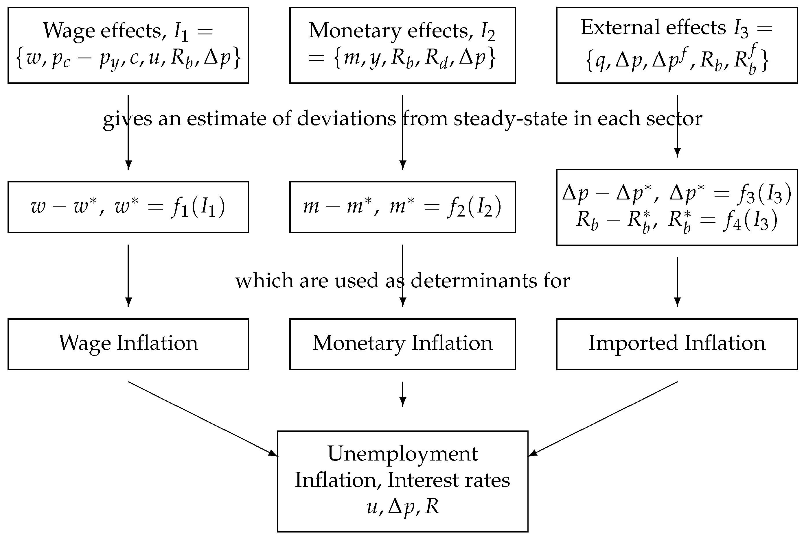
To circumvent this problem, Juselius (1992) proposed a procedure for combining partial models into a larger macro model. The idea was to study how CPI inflation was affected by monetary inflation, wage inflation, and imported inflation by estimating cointegration relations in three partial VAR models. Econometrically, the procedure is based on the invariance of the cointegration property to expansions of the information set. Economically, it rests on the interpretation of a properly identified cointegration relation as a deviation from a long-run equilibrium value, implying that it could be treated as a convenient summary measure of the most important information from the sector in question. For example, if wages at time t are on the equilibrium level, then the value of the cointegration relation would be approximately zero, implying no wage pressure on CPI inflation. In contrast, if the absolute value of the cointegration relation is large, then wages are either below or above their equilibrium level with a potentially large impact on CPI inflation.
I used the same idea in Juselius (2006, Part VI) where more detailed and extensive analyses of the three sectors are reported. Figure 1 below illustrates the procedure. First, the relevant long-run relations are identified based on smaller CVAR models, then the deviations from these relations enter as the main explanatory variables in a bigger model explaining key economic determinants, such as CPI inflation, the unemployment rate and the interest rate8. The list of key variables can of course be extended as illustrated in Juselius (2006, chp. 22). For the period 1972–2003, the results showed that (i) the identified cointegration relations represented the major bulk of the explanatory power with only minor effects from short-run changes of the system variables, (ii) excess money had essentially no effect on the CPI inflation rate, (iii) wage inflation had a large inflationary effect until capital deregulation in the mid-eighties and only a modest effect afterwards, and (iv) wage increases reflected a smaller part of the productivity growth after globalization and capital deregulation than before. Labor unions seemed to have become increasingly powerless.
While not perfect, the results from the big combined model seemed very promising. The idea of using the “specific-to-general” in the choice of information set and the “general-to-specific” in the search for a parsimoniously parametrized model begun to look like a feasible way to overcome both the dimensionality problem of the CVAR and the complexity problem of large macro models.
I was excited about the possibility to use the above principle to handle large scale macro models, such as the traditional Keynesian macro models consisting of numerous behavioral relations in which endogeneity, exogeneity, and ceteris paribus are given a priori. Such a behavioral relation could be subject to a CVAR analysis without the need to fix the status of a variable as endogenous or exogenous and with the possibility to add relevant ceteris paribus variables. Furthermore, the stationarity of the presumed behavioral relations could be properly tested and efficiently estimated, dynamic feedback effects and long-run dynamic multiplier effects would be readily available.
By combining such partial dynamic models into a large-scale model of the economy, one would obtain something resembling a general (dis)equilibrium macromodel. It would be based on the assumption that deviations from equilibrium values—the equilibrium errors—are the most crucial determinants of key variables in the economy, such as output growth, unemployment, wage inflation, interest rate, CPI inflation, house price inflation, stock price inflation, and real exchange rate. At the same time it would provide useful information about the dynamics of each subsector of the economy. I thought it would give large-scale macro models a much needed face lift and be a powerful method for an improved understanding of our complex economic reality. To my disappointment the idea has not yet been realized anywhere in the world, at least not to my knowledge.
5. Towards a New Methodological Approach
After having applied the CVAR to numerous empirical problems, it became ever more evident that there was more persistence in the data than standard models could explain. I often found the data to be indistinguishable from and this was not just for price variables, like the CPI, but also for relative prices, nominal and real exchange rates, and even real and nominal interest rates, which a priori were expected to be stationary or at most . Even unemployment, another important real economy variable, was often found to be indistinguishable from and cointegrated with the real interest rate and the real exchange rate.
Many economists would argue that such findings are implausible as economic variables could not drift away forever as a true process can, nor could equilibrium errors be as economic variables do not move infinitely away from their equilibrium values. However, while this is obviously correct, it does not exclude the possibility that variables over finite samples may exhibit a persistence that is empirically indistinguishable from a unit root or a double unit root process. Furthermore, because economic relationships seldom remain unchanged for long periods of time, the infinity argument may not be very relevant in economics. In line with this, Juselius (2013) argues that a statistical unit root should not be given an interpretation as a structural economic parameter and that the classification of variables/relations as either stationary, (near) or (near) is a requisite for successful empirical modeling.
What makes a near process extremely interesting is that such a process is able to generate long-lasting swings, a typical feature of economic variables (Johansen 1997, 2006; Paruolo and Rahbek 1999). In spite of this, applications of the model are rare in the literature. To understand why, Juselius (2014) discusses a simple case, where and the shocks are small compared to the shocks i.e., the signal-to-noise ratio is small. Simulations show that univariate Dickey–Fuller tests hardly ever detect the second unit root in the drift term, whereas the multivariate tests almost always find it. This is particularly so when the signal-to-noise-ratio is small, typical of asset prices in speculative markets. As most people use univariate rather than multivariate tests to determine the order of integration, the results may explain why econometricians/economists find economic variables/relations to be rather than .
Why is this important? Knowing the approximate order of integration and cointegration among variables is a very important and useful piece of information in the modelling process. For example, an variable cannot be significantly related to an variable, neither can an variable to an variable, but they can be combined to form a stationary cointegrated relationship. Therefore, by exploiting the information in the data given by the integration/cointegration properties of the variables, one can obtain robust estimates of long-run, medium-run, and short-run structures in the data, thus improving the specification of the economic model. In the words of Hoover et al. (2009), the CVAR allows the data to speak freely about the mechanisms that have generated them. Juselius (2006, 2013) provide more detailed discussions.
5.1. Long Swings in Financial Market Behavior
At that time, financial behavior was rarely part of macroeconomic models as—somewhat simplistically—a fully rational financial actor was assumed to know when the market price deviated from its equilibrium price and then would act accordingly. Rational financial markets would, therefore, drive financial prices back to equilibrium and the equilibrium prices would correctly reflect movements in the real economy. Because financial prices were assumed to be correctly determined, deregulated financial markets were good, not harmful, to the real economy. Therefore, there was no need to regulate and no reason to worry about the effect of financial market behavior in macroeconomic models. The reasoning relied on the efficient market hypothesis, that was based on the rational expectations hypothesis and the assumption that economic models are known and stable over time. However, all these assumptions seemed at odds with what I constantly saw in the data: the frequent structural breaks, the frequent changes of exogeneity status, the long and persistent swings around equilibrium values indistinguishable from a unit root process.
That the deviations from some of the fundamental economic parities—the Fisher parity, the term spread, the purchasing power parity, the uncovered interest rate parity—were statistically indistinguishable from unit root processes seemed particularly worrisome to me. Where did this additional persistence come from? It seemed inconsistent with standard REH models which assumed much faster adjustment to long-run equilibria. Why did the persistent swings not vanish with the nominal-to-real transformation when the nominal deflator was the consumer price index? It gradually dawned on me that long and persistent swings in both the nominal and the real magnitude of a variable were typically found in prices associated with financial behavior, such as exchange rates, interest rates, stock prices, house prices, energy prices, and prices for precious metals. It raised the question why did they fluctuate in a manner detached from the development of standard consumer prices and real productivity growth in the economy?
As already mentioned, this empirically very strong feature turned out to be largely consistent with a monetary model for the exchange rate based on imperfect knowledge expectations (Frydman and Goldberg 2007, 2011). The imperfect knowledge argument is that no one can know—not even in probabilistic terms—what the true fundamental value of an asset is. This is because the value of a financial asset is a function of future—unpredictable—cash flows. Given such Knightian uncertainty, market participants interpret in diverse ways a wide range of news about fundamental factors, from real growth and inflation rate announcements to political developments and debt crises. This diversity combined with loss aversion can then explain why forecasts of future asset prices tend to generate persistent movements around benchmark values.
The theory of imperfect knowledge economics provided me with an explanation of the puzzling finding that the real exchange rate and the real interest rate differential were empirically near . In Frydman et al. (2008, 2012) we addressed the PPP puzzle and the long swings puzzle both theoretically and empirically.
Another strain was offered by Hommes (2006) and Hommes et al. (2005a, 2005b), which similarly focus on the persistent swings in asset prices. In this theory, financial markets are populated by fundamentalists using economic fundamentals to forecast future price movements, and by chartists—trend-followers—using technical trading rules to forecast prices. Financial actors are switching endogenously between mean-reverting fundamentalists and trend-following chartists depending on how far away the price is from long-run equilibrium values. Positive feedback prevails when the chartists dominate the market and negative feed-back when the fundamentalists dominate.
Common to the above models is that today’s asset price depends on future prices which, in varying degree, are being forecasted under imperfect knowledge and, therefore, deviate from the price derived under the REH. In both models prices can deviate from long-run benchmark values for extended periods of time, thereby generating self-reinforcing expectational cycles. All this seemed to provide a rational for my puzzling findings and was a motivation to focus on financial behavior and its role for the real economy.
5.2. Persistent Movements and Time-Varying Coefficients
How to analyze such self-reinforcing expectational cycles econometrically is, however, far from simple. Inspired by (Frydman and Goldberg 2007, 2011), Juselius and Assenmacher (2017) interpreted the long swings in the real US dollar-Swiss franc rate in the context of a simple model with time-varying coefficients using the following assumptions: A financial actor understands that PPP holds in the long run, but not necessarily in the short run. He/she is, therefore, in the short-term likely to react on a number of other determinants, such as changes in interest rates, relative incomes and consumption, and many more. In such a world, financial actors tend to attach time-varying weights, to relative prices depending on how far away the nominal exchange rate is from its fundamental PPP value, i.e.,
where is the log of the nominal exchange rate, is the log of the relative price between domestic and foreign country, and fluctuates around 1.0. The change in the nominal exchange rate can then be expressed as
where can be assumed very small. In addition, Frydman and Goldberg (2007) makes the assumption that This is backed up by simulations showing that a change in has to be implausibly large for to have a noticeable effect on Therefore,
where and are typically near processes. To study the properties of this type of time-varying parameter model, Tabor (2014) considered the CVAR model:
He generates the data with and where Then, for implies that the adjustment of back to is immediate. Instead of estimating a time-varying parameter model, Morten fitted a constant parameter CVAR model to the simulated data, so that becomes part of the CVAR residual. The results in Tabor (2014) show that the closer is to 1, the more persistent is the estimated gap term, , and the smaller is the estimated adjustment coefficient —albeit still highly significant. Furthermore, as long as the mean of the estimated approximately equals its true value . When this is no longer the case.
Thus, the pronounced persistence away from long-run equilibrium values and the small adjustment coefficients often found in constant-parameter CVAR models is potentially a result of time-varying coefficients due to forecasting under imperfect knowledge. Juselius (2017) shows that this may explain the persistence of the PPP gap and the inability to reject persistence using the CVAR. Even though under this assumption, the model is just an approximation of a model with time-varying coefficients, it may, nonetheless, be a useful approximation. The linear VAR with constant parameters gives access to a vast econometric literature on estimation and testing, whereas the complexity of estimating a time-varying parameter VAR model is daunting except for small models with only one or a few time-varying parameters.
When analyzing the PPP and the UIP conditions for various countries based on CVAR models, the results frequently supported the main assumption of the imperfect knowledge based monetary model that the deviations from the PPP was cointegrated with the spread between the domestic and foreign real interest rates. By interpreting the persistent movements in the real exchange rate as a proxy for an uncertainty premium in the foreign currency market—proposed by Frydman and Goldberg (2007)—the results show strong empirical support for a stationary uncertainty adjusted UIP condition. Furthermore, Johansen et al. (2010) reported an econometric analysis of the full set of international parity conditions using German—US data.
Juselius and Assenmacher (2017) also report a similar study of Swiss-US data in which equilibrium error-increasing behavior is used to identify the channels through which self-reinforcing feedback mechanisms takes place. The results show that such behavior plays a significant role for the persistent fluctuations in exchange rates, interest rates, and prices. They also show that once loss-aversion and uncertainty is allowed for, the excess return puzzle disappears, suggesting that agents are behaving rationally but that imperfect knowledge outcomes are very different from the ones in an REH world.
5.3. Real Exchange Rate Persistence and the Real Economy
The derived CVAR scenario for an imperfect knowledge monetary model in Juselius (2017) provides an explanation for why asset prices, but not CPI prices, tend to fluctuate in long persistent swings and, consequently, why real trend-adjusted asset prices are empirically almost indistinguishable from their nominal trend-adjusted magnitudes, and why interest rate differentials are near . The imperfect knowledge-based monetary model fits the data remarkably well as shown in Juselius (2006, chp. 21) for Denmark versus Germany, Juselius and MacDonald (2004) for Japan versus USA, Juselius and MacDonald (2006) for Germany versus USA, Juselius and Assenmacher (2017) for Switzerland versus USA, and Juselius and Juselius and Stillwagon (2018) for UK versus USA.
Common to the above papers is the finding that Purchasing Power Parity needs Uncovered Interest Parity to become a stationary parity relation. The implication is that equilibrium in the goods market is not directly associated with purchasing power parity but with a stationary relation between a nonstationary real exchange rate and the interest rate spread. Thus, the real exchange rate can persistently appreciate/depreciate as long as the real interest rate differential moves in an offsetting manner. As these persistent swings around equilibrium values are caused by speculative behavior in the market for foreign exchange, they are essentially outside domestic policy control—at least as long as transactions in the foreign currency market are neither regulated nor taxed.
For the US dollar and the UK pound market, Juselius and Stillwagon (2018) found that it is the interest rate expectations—measured by consensus forecasts of professional forecasters—that are pushing the interest rates and the exchange rate in the long run. Furthermore, the results show that it is the shocks to the US consensus forecasts—rather than the UK ones—that are dominating the long persistent swings. An interesting finding is that changes in the nominal exchange rate are pushing the foreign currency market in the medium run with interest rates following suit, whereas expectational shocks to the interest rates are pushing the market in the long run with the nominal exchange following suit. These results are basically consistent with imperfect knowledge based models.
That the fundamental parity conditions—in particular the PPP and the UIP—were systematically found to be non-stationary, prompted the question of how this is affecting the real economy.
Juselius (2013) was my first attempt to address the two-way interdependence between the real economy and financial behavior in asset markets. The theme of the paper was strongly influenced by Phelps’ hypothesis that the natural rate of unemployment is a function of the real interest rate and/or the real exchange rate. Because Phelps’ “Structural Slumps” book assumed the latter to be stationary, I was excited to examine the implications of them being nonstationary instead.
In a stationary world, exporting and importing enterprises would be insulated from changes in the relative costs, if the nominal exchange rate correctly reflects relative costs between the two countries. In a nonstationary world, where the nominal exchange rate is typically determined by speculative transactions, it is much less affected by the trade in exports and imports.9 Thus, an exporting firm would have to resort to “pricing-to-market” strategies rather than mark-up-pricing (Krugman 1986), or it would lose market shares. For example, over a prolonged period of currency appreciation, such a firm will experience a mounting pressure to be competitive. As raising the price is not feasible, there are few other options than to improve productivity. This can be done, for example, by requiring workers to produce more per hour, firing the least productive workers, outsourcing production, or introducing new technology. All these measures affect unemployment rate. When the exchange rate finally reverses—now depreciating—the pressure on competitiveness is released but, because competing enterprises in foreign countries now experience an appreciating exchange rate and, therefore, have to resort to similar measures, prices do not rise much.
Thus, consumer prices—determined by fierce competition in an international market—remain low and stable, whereas asset prices—determined by speculative expectations—tend to fluctuate in long persistent swings. The fact that the unemployment rate and trend-adjusted productivity have been co-moving and that the natural rate of unemployment has been a function of the real interest rate—rather than a constant—are consistent with the above mechanisms (Juselius 2006, chp. 20; Juselius and Ordóñez 2009).
These results can also explain the inflation puzzle, e.g., why inflation has been low and stable over time (below 2% for several decades) at the same time as the nominal interest rate has moved in long persistent swings and, hence, why CPI inflation and nominal interest rate are typically not found to be cointegrated, against the Fisher parity assumption.
They also suggest that any attempt to control inflation by changing central bank interest rate is likely to be ineffective. To be effective, such a policy rule would require the above parities to hold as stationary conditions, or important parts of the transmission mechanism are broken. Evidence of this was found in Johansen and Juselius (2001) in which the Federal Funds rate was shown to be an inefficient instrument for US inflation control during the Greenspan monetary policy period. While the inflation rate has been low in periods of inflation targeting, my claim is—supported among others by the CVAR analyses in Juselius (1998b)—that it has been so for other reasons, primarily financial deregulation and global competition.
One consequence of the low inflation rate is that the pressure on the central bank to raise its interest rate has been low for several decades. Exceptionally low interest rate levels have in turn led to easy credit and a corresponding strong increase in liquidity. The consequence of high, credit-financed, demand for real estate and stock is that house and stock prices have sky-rocketed. At the same time, the CPI inflation rate has remained low. Juselius (2019) reports a comprehensive analysis of the soaring Danish house and stock prices, totally detached from the CPI prices and the real GDP, that ultimately led to the Danish house price bubble in 2007 and then to the financial crisis in 2008.
Juselius (2019) demonstrates empirically that accruing imbalances often tend to counterbalance each other, sometimes over extended periods of time and argues that a balance maintained by several imbalances is a very fragile balance: sooner or later a large shock to the system will cause the balance to collapse—as happened in 2007 when the house price bubble burst and similarly in 2008 when the financial crisis hit the world economy with unprecedented force. Thus, the great recession seems to have grown out of many imbalances—initiated by financial behavior—which were allowed to develop over a long time.
Over time I have become ever more convinced that financial behavior is an extremely important determinant of the real economy. This was also the main conclusion in Colander et al. (2009) which already in 2008 argued that unrealistic financial models have had a large and detrimental effect on real economies. A few months later, this claim turned out to be almost too correct.
5.4. Crises Periods and Comparative Studies
At a time when many argued that the Great Recession was a once in a life time event—a black swan—that could not have been foreseen, I vividly remembered a similar crisis at the beginning of the nineties in Finland. The deregulation of the Finnish credit market in 1986 had resulted in an overheated economy and in strongly increasing real estate prices. When the house price bubble burst, unemployment rates soared and reached more than 20%—from a starting position of 1.6%—in a very short period of time. In a joint project with my son Mikael Juselius (Juselius and Juselius 2013), we asked the questions (i) whether the Finnish experience could be understood as a balance sheet recession10, (ii) whether the unemployment dynamics made sense in the context of Phelps’ Structural Slumps theory (Phelps 1994), and (iii) whether the theory of Imperfect Knowledge Economics (Frydman and Goldberg 2007, 2011) could explain the persistent movements in the data. To answer these questions, we applied the CVAR model to inflation, unemployment, a short- and a long-term interest rate.
Econometrically, our CVAR model performed surprisingly well—considering the wild fluctuations of the Finnish data. The results—reported in Juselius and Juselius (2013)—gave support to all three priors: the Phelps’ hypothesis that the natural rate of unemployment is a function of the real interest rate; the Frydman and Goldberg Imperfect Knowledge hypothesis of pronounced persistence in the long-term real interest rate; and the Koo hypothesis of the Central Bank interest rate as an ineffective instrument during a balance sheet recession. Furthermore, based on a smooth transition model in which the transition variable was designed to capture household sector leverage—adjusted for movements in the value of the housing collateral, the paper demonstrated that strongly increasing house prices had played a crucial role for the depth and the length of the subsequent crisis. As soon as house prices started falling and the house debt exceeded the value of the collateral, the leverage effect was shown to become extremely important.
Altogether, the Finnish results seemed to be able to shed light on the dynamic transmission mechanisms of inflation, unemployment and interest rates in a crisis period. It raised the question whether the results could have been used to foresee the housing bubble 15 years later, or whether there were lessons to be learned for other countries with a similar bubble experience. The latter was the underlying motivation in Juselius and Dimelis (2019) to address the empirical mechanisms governing the Greek depression, the most serious and destructive of all European crises.
Many aspects of the Finnish crisis were similar to the ones in Greece: the deregulation of the Finnish credit market in 1986 resulted in a booming housing market and a serious house price bubble; joining the eurozone caused the Greek bond rate to drop to previously unprecedented levels and caused a credit financed boom in aggregate demand. As in Finland, Greek wages and prices—in particular real estate prices—were rising and competitiveness was deteriorating. When the Greek bubble burst, the drop in aggregate income and the rise in unemployment rate were huge and of similar magnitudes as in Finland. However, the Greek crisis, while similar in many aspects to the Finnish one, differs strongly in others. For example, the source of the debt (private/public, external/internal), the strong/weak institutional set-up, and in particular the exchange rate regime are defining differences of crucial importance. The fact that Finland was able to devalue its currency while Greece was not, is likely to have made all the difference for the length of the crisis. It is one reason why the comparison with Finland is interesting.
Unlike the Greek economy, Finland managed to get out of the crisis in approximately three—admittedly very hard—years by devaluing the Finnish markka with 33%. Moreover, unlike the Greek experience, the Finnish unemployment rate came down quite fast, albeit stabilizing at a somewhat higher level compared to the pre-crisis period. One reason why the Greek unemployment was stuck at very high levels seemed to be the prolonged period of policy uncertainty following the outbreak of the crisis. Unlike the Finnish analysis, the Greek analysis therefore required a variable measuring confidence as well as two variables measuring the development of the Greek competitiveness within and outside the eurozone.
In the Greek analysis, the most striking result was a critical relationship between the bond rate and the unemployment rate: As the crisis erupted, the bond rate increased sharply followed by a strong increase in unemployment, the increase in unemployment rate caused the bond rate to increase further and unemployment to follow suit, and so on. This vicious cycle was orchestrated by a continuous fall in the confidence rate that kept deteriorating until relative producer costs stopped increasing around 2012. The empirical results showed that all variables, except CPI inflation, exhibited self-reinforcing feedback behavior somewhere in the system, a feature that is likely to have aggravated the problems and effectively prevented good policy solutions. As the euro rate was determined by factors mainly outside the Greek control, Greece was stuck in a situation with no feasible options: a dramatic lowering of wage costs was politically impossible; leaving the euro would have been extremely costly due to the large external debt. At the same time the confidence in the Greek economy continued to drop which added to the depressed state of the economy.
The two papers illustrate an important methodological principle: by using the same “experimental design”, here the CVAR model, and controlling for institutional differences by conditioning on appropriately selected variables, one can learn about similarities and dissimilarities in different economies. I thought this would be particularly valuable when addressing policy changes and the response to them.
Juselius et al. (2014) followed a similar principle when studying the effectiveness of foreign aid in 36 South Saharan African countries. Among these, 29 countries were classified into four more homogeneous groups according to aid effectiveness11. Within these groups more detailed analyses were performed. The results showed that the overall qualitative conclusions were rather similar for the vast majority of South Saharan African countries. However, the results also showed that the dynamics of the transmission of aid onto the macro economy differed a lot depending on the classification. This was not surprising as such: aid is given for different purposes in different countries. Econometrically, our results pointed to the peril of using panel data analyses as a basis for policy advice in such diverse countries as South Saharan African countries. As aid effectiveness has frequently been studied based on panel data analyses which—implicitly or explicitly—assume homogeneous countries across the panel, this should be a reason for concern.
A small number of countries fell outside the classification criteria, among them Ghana and Tanzania. Based on an extended data set, Juselius et al. (2017) studied the transmission mechanisms of aid in more detail for these two countries. It turned out that both countries—for political reasons—had manipulated their exchange rate for extended periods of time, with the consequence that the aid transmission mechanism did not follow a standard pattern. Conditional on the anomalous exchange rate regimes, the aid transmission results became economically interpretable again. Yet another example of the importance of the ceteris paribus clause.
The three papers in this section and many others mentioned earlier serve the purpose of illustrating the potential of the CVAR as a design of experiment for data obtained by passive observations. Perhaps it is time to challenge the frequent claim that it is not possible to apply designed experiments in macroeconomics.
6. Some Reflections
The title of this paper “Searching for a theory that fits the data” was chosen to emphasize the distinction between my own empirical approach and the one that underpins most empirical research in economics: “Searching for data that fits the theory”. This difference reflects, no doubt, what the researcher considers most important: the empirical reality or the theory supposed to explain it. For me it was never a choice: to better understand what was going on in the empirical economy was the main reason why I chose a university career in economics. To develop empirical methods that could increase the transparency of economic mechanisms and potentially improve economic policy decisions has been an important personal driver in all these years of extremely hard work.
To stumble over the CVAR and see its great potential as a methodology for empirical economics was like winning a lottery. However, while I believe the CVAR has fully lived up to its promises, the way it has been applied in the literature has been disappointing. Numerous papers report all kind of CVAR analyses, most of them give the impression of being done by statistical non-experts: data have been read in and the CVAR button has been pushed. However, the CVAR methodology cannot be applied mechanically: it depends upon the researcher’s statistical expertise and requires interaction between the econometrician, the economist and the data. For example, it does not make sense to work with a CVAR model until you have checked whether (1) the sample period is representative for your questions, (2) the chosen information set is sufficiently broad to answer the questions of interest, (3) the most important institutional changes have been controlled for, (4) the parameters of interest are reasonably stable over time, (5) the residual mis-specification tests are acceptable, and many more. If you sidestep these important steps, you will very likely get nonsense. Perhaps this is the reason why the impact of the CVAR on economic modeling has been so disappointing.
A frequent claim is that the quality and informational content of macroeconomic data are too low for a CVAR analysis to be reliable. I agree that economic time series data seldom represent the true measurements of the theoretical model. For example, the representative agent’s income, consumption, and hours worked in a DSGE model has little in common with the various measurements of aggregate income, private consumption, and total hours worked that can be found in the national statistical publications. However, while macro data are clearly contaminated with measurement errors, such errors may not be of great concern for the more important long-run analysis unless they are systematic and cumulate to a nonstationary process. Whatever the case, theoretically correct measurements do not exist and, thus, cannot be used by politicians and decision makers to react on. The forecasts, plans and expectations that agents base their decisions on are the observed data and we better understand them, however imperfect they are.
A related claim is that, unless the empirical model is constrained by theory from the outset, one would not be able to make sense of the results: without the mathematical logic of the theoretical model, one opens up for quackery. I hold the opposite view. Scientific objectivity can only be achieved provided data are not constrained from the outset in a theoretically prespecified direction. When they are, it is impossible to know which results are due to the assumptions made and which are true empirical findings. This point was amply illustrated in Juselius and Franchi (2007) where essentially all assumptions underlying a DSGE model by Ireland (2004) were found to lack empirical support. When a well-specified CVAR was fitted to the same data the results showed that all conclusions were reversed. Thus, the conclusions of the Ireland paper reflect the assumptions made rather than true empirical findings.
Another related claim is that CVAR models are so general that they can show anything.12 Over time, I have applied the CVAR model to numerous problems in a variety of countries and for many different time periods. These applications have convinced me that macroeconomic data are surprisingly informative, but only if you let them speak freely about the story they want to tell. This, of course, does not mean that data can speak by themselves without theory, nor without rigor: a CVAR analysis should obey equally strict rules as a mathematical analysis of an economic model. A well-specified CVAR model, estimated by a full information maximum likelihood method, describes by definition all aspects of the data and, thus, summarizes the empirical features that an empirically relevant theory should be able to explain. Typical features are unit root nonstationarity, structural change, non-constant parameters, dynamic long-run equilibrium relationships, and self-reinforcing feedback mechanisms. All of them have strong implications for the choice of economic model. For example, nonstationarity is consistent with economic relations that deviate persistently—in a near manner—from long-run equilibria, suggesting that the choice of economic model should be based on disequilibrium economics. Guzman and Stiglitz (2020) discuss the basic features of such a theory.
Disequilibrium economics again points to complex adjustment dynamics and nonstandard—non-REH—expectations as the relevant concepts. Data covering crises periods typically reveal such features. While many economists consider crisis periods to be aberrations outside the range of economic modeling, they are not outside the range of a well-specified CVAR analysis. Economic crises are often devastating for ordinary people’s lives and any lesson that can be learned should not be missed. In 2008, standard mainstream models did not spot the accruing imbalances and, hence, failed to prevent and explain the economic crisis. As these models are still based on essentially the same assumptions, it seems unlikely that they will be able to foresee the next crisis in time to prevent it. See also the critique in Stiglitz (2018).
The CVAR results have typically favored traditional Keynesian macroeconomics, albeit modified with expectations based on uncertainty and imperfect knowledge and controlling for the effect of financial behavior. As the dynamic macroeconomic disequilibrium theory proposed in Guzman and Stiglitz (2020) is broadly in line with the above, I argue in Juselius (2021b) that the CVAR may have the potential to work as an empirical methodology for disequilibrium macroeconomics. The fact that the many—then theoretically puzzling—CVAR results reported in Section 4 would no longer be puzzling in the context of disequilibrium economics, should contribute to the plausibility of this suggestion.
I will end the tale of my personal odyssey by hoping that this journey, bending and looping as it has been, can convince at least some econometricians, economists and policy-makers that well-founded empirical findings rather than theoretical convictions should guide economic policy. The abundance of theoretically puzzling—but empirically and econometrically well founded results—signal the need for new theory and deserve to be taken seriously. No doubt, empirically unfounded economic policy is likely to have exacerbated some of the defining problems of our time, such as recurring crises, increasing inequality, and growing populism. The development of a more relevant macroeconomics that serve not just the few but all is desperately needed.
Funding
This research received no external funding.
Institutional Review Board Statement
Not applicable.
Informed Consent Statement
Not applicable.
Data Availability Statement
The data presented in this study are available on request from the corresponding author. The data are not publicly available due to privacy.
Acknowledgments
I would like to thank the guest editors, Rocco Mosconi and Paolo Paruolo, for asking me to prepare a survey paper of my past and ongoing research. I was very happy to accept it. In all these years, the Danish Social Sciences Research Council has generously supported my research with several grants. In the last years prior to my retirement, I was fortunate to obtain a Centre grant from the Institute of New Economic Thinking. I am thankful for all the support I obtained. I am also grateful for valuable comments from two anonymous referees, from the two guest editors, and from Michael Goldberg and Roman Frydman.
Conflicts of Interest
The author declares no conflict of interest.
References
- Colander, David, Michael Goldberg, Armin Haas, Katarina Juselius, Alan Kirman, Thomas Lux, and Birgitte Sloth. 2009. The Financial Crisis and the Systemic Failure of the Academics Profession. Critical Review 21: 249–67. [Google Scholar] [CrossRef]
- Dennis, Jonathan, Henrik Hansen, Søren Johansen, and Katarina Juselius. 2006. CATS in RATS. Cointegration Analysis of Time Series. Version 2. Evanston: Estima. [Google Scholar]
- Doornik, Jonathan, and Katarina Juselius. 2017. Cointegration Analysis of Time Series Using CATS 3 for OxMetrics. New York: Timberlake Consultants Ltd. [Google Scholar]
- Engle, Robert, David Hendry, and Jean-Francois Richard. 1983. Exogeneity. Econometrica 51: 277–304. [Google Scholar] [CrossRef]
- Friedman, Milton. 1970. The Counterrevolution in Monetary Theory. Occasional paper 33. London: Institute of Economic Affairs. [Google Scholar]
- Frydman, Roman, and Michael Goldberg. 2007. Imperfect Knowledge Economics: Exchange Rates and Risk. Princeton: Princeton University Press. [Google Scholar]
- Frydman, Roman, and Michael Goldberg. 2011. Beyond Mechanical Markets: Risk and the Role of Asset Price Swings. Princeton: Princeton University Press. [Google Scholar]
- Frydman, Roman, Michael D. Goldberg, Søren Johansen, and Katarina Juselius. 2008. A Resolution of the Purchasing Power Parity Puzzle: Imperfect Knowledge and Long Swings. Working Paper 31. Copenhagen: Economics Department, University of Copenhagen. [Google Scholar]
- Frydman, Roman, Michael Goldberg, Søren Johansen, and Katarina Juselius. 2012. Long Swings in Currency Markets: Imperfect Knowledge and I(2) Trends. Copenhagen: University of Copenhagen. [Google Scholar]
- Granger, Clive. 1983. Cointegrated Variables and Error Correction Models. Discussion Paper. San Diego: University of California. [Google Scholar]
- Guzman, Martin, and Joseph Stiglitz. 2020. Towards a Dynamic Disequilibrium Theory with Randomness. Working Paper 27453. Cambridge: National Bureau of Economic Research. [Google Scholar]
- Haavelmo, Trygve. 1944. The Probability Approach to Econometrics. Econometrica 12: 1–118. [Google Scholar] [CrossRef]
- Hansen, Henrik, Søren Johansen, and Katarina Juselius. 1994. CATS in RATS. Version 1.0. In Manual to Cointegration Analysis of Time Series. Evanstone: ESTIMA. [Google Scholar]
- Hendry, David, and Katarina Juselius. 2000. Explaining Cointegration Analysis. Part 1. The Energy Journal 21: 1–42. [Google Scholar] [CrossRef]
- Hendry, David, and Katarina Juselius. 2001. Explaining Cointegration Analysis. Part 2. The Energy Journal 22: 1–52. [Google Scholar] [CrossRef] [Green Version]
- Hommes, Cars. 2006. Heterogeneous Agent Models in Economics and Finance. In Handbook of Computational Economics 2. Edited by Leigh Tesfation and Kenneth Judd. Amsterdam: Elsevier. [Google Scholar]
- Hommes, Cars, Hai Huang, and Duo Wang. 2005a. A Robust Rational Route to Randomness in a Simple Asset Pricing Model. Journal of Economic Dynamics and Control 29: 1043–72. [Google Scholar] [CrossRef] [Green Version]
- Hommes, Cars, Joep Sonnemans, Jan Tuinstra, and Henk van der Velden. 2005b. Coordination of Expectations in Asset Pricing Experiments. Review of Financial Studies 18: 955–80. [Google Scholar] [CrossRef]
- Hoover, Kevin, Søren Johansen, and Katarina Juselius. 2009. Allowing the Data to Speak Freely: The Macroeconometrics of the Cointegrated Vector Autoregression. American Economic Review 98: 251–55. [Google Scholar] [CrossRef] [Green Version]
- Hoover, Kevin D., and Katarina Juselius. 2015. Trygve Haavelmo’s Experimental Methodology and Scenario Analysis in a Cointegrated Vector Autoregression. Econometric Theory 31: 249–74. [Google Scholar] [CrossRef] [Green Version]
- Ireland, Peter. 2004. A Method for Taking Models to the Data. Journal of Economic Dynamics & Control 28: 1205–26. [Google Scholar]
- Johansen, Søren. 1988. Statistical Analysis of Cointegration Vectors. Journal of Economic Dynamics and Control 12: 231–54. [Google Scholar] [CrossRef]
- Johansen, Søren. 1992. Cointegration in Partial Systems and the Efficiency of Single Equation Analysis. Journal of Econometrics 52: 389–402. [Google Scholar] [CrossRef]
- Johansen, Søren. 1994. The Role of the Constant and Linear Terms in Cointegration Analysis of Non-Stationary Variables. Econometric Reviews 13: 205–30. [Google Scholar] [CrossRef]
- Johansen, Søren. 1996. Likelihood-Based Inference in Cointegrated Vector Autoregressive Models. Oxford: Oxford University Press. [Google Scholar]
- Johansen, Søren. 1997. Likelihood Analysis of the I(2) Model. Scandinavian Journal of Statistics 24: 433–62. [Google Scholar] [CrossRef]
- Johansen, Søren. 2006. Statistical Analysis of Hypotheses on the Cointegrating Relations in the I(2) Model. Journal of Econometrics 132: 81–115. [Google Scholar] [CrossRef]
- Johansen, Søren, and Katarina Juselius. 1990. Maximum Likelihood Estimation and Inference on Cointegration—With Applications to the Demand for Money. Oxford Bulletin of Economics and Statistics 52: 169–210. [Google Scholar] [CrossRef]
- Johansen, Søren, and Katarina Juselius. 1992. Testing Structural Hypotheses in a Multivariate Cointegration Analysis of the PPP and the UIP for UK. Journal of Econometrics 53: 211–244. [Google Scholar] [CrossRef]
- Johansen, Søren, and Katarina Juselius. 1994. Identification of the Long-Run and Short-Run Structure: An Application to the ISLM Model. Journal of Econometrics 63: 7–36. [Google Scholar] [CrossRef]
- Johansen, Søren, and Katarina Juselius. 2001. Controlling Inflation in a Cointegrated Vector Autoregressive Model with an Application to US Data. Working Paper 3. Copenhagen: University of Copenhagen. [Google Scholar]
- Johansen, Søren, and Katarina Juselius. 2006. Extracting Information from the Data: A European View on Empirical Macro. In Post Walrasian Macroeconomics: Beyond the Dynamic Stochastic General Equilibrium Model. Edited by David Colander. Cambridge: Cambridge University Press, pp. 301–33. [Google Scholar]
- Johansen, Søren, and Katarina Juselius. 2014. An Asymptotic Invariance Property of the Common Trends under Linear Transformations of the Data. Journal of Econometrics 178: 310–15. [Google Scholar] [CrossRef]
- Johansen, Søren, Katarina Juselius, Roman Frydman, and Michael D. Goldberg. 2010. Testing Hypotheses in an I(2) Model with Piecewise Linear Trends. An Analysis of the Persistent Long Swings in the Dmk/$Rate. Journal of Econometrics 158: 117–29. [Google Scholar] [CrossRef]
- Johansen, Søren, and Anders Rygh Swensen. 1999. Testing Exact Rational Expectations in Cointegrated Vector Autoregressive Models. Journal of Econometrics 93: 73–91. [Google Scholar] [CrossRef]
- Johansen, Søren, and Anders Rygh Swensen. 2004. More on Testing Exact Rational Expectations in Cointegrated Vector Autoregressive Models: Restricted Constant and Linear Term. The Econometrics Journal 7: 389–97. [Google Scholar] [CrossRef]
- Juselius, Katarina. 1992. Domestic and Foreign Effects on Prices in an Open Economy: The Case of Denmark. Journal of Policy Modeling 14: 401–28. [Google Scholar] [CrossRef]
- Juselius, Katarina. 1993. VAR Modelling and Haavelmo’s Probability Approach to Macroeconomic Modelling. Empirical Economics 18: 595–622. [Google Scholar] [CrossRef]
- Juselius, Katarina. 1994. On the Duality Between Long-Run Relations and Common Trends in the I(1) versus I(2) Model: An Application to Aggregate Money Holdings. Econometric Reviews 13: 151–79. [Google Scholar] [CrossRef]
- Juselius, Katarina. 1995. Do Purchasing Power Parity and Uncovered Interest Rate Parity Hold in the Long Run? An Example of Likelihood Inference in a Multivariate Time-Series Model. Journal of Econometrics 69: 211–40. [Google Scholar] [CrossRef]
- Juselius, Katarina. 1996. An Empirical Analysis of the Changing role of German Bundesbank after 1983. Oxford Bulletin of Economics and Statistics 58: 791–817. [Google Scholar] [CrossRef]
- Juselius, Katarina. 1998a. A Structured VAR for Denmark under Changing Monetary Regimes. Journal of Business and Economic Statistics 16: 400–11. [Google Scholar]
- Juselius, Katarina. 1998b. Changing Monetary Transmission Mechanisms within the EU. Empirical Economics 23: 455–81. [Google Scholar] [CrossRef]
- Juselius, Katarina. 1999a. Price Convergence in the Long Run and the Medium Run. An I(2) analysis of six price indices. In Cointegration, Causality, and Forecasting. Festschrift in Honour of Clive Granger. Edited by Robert Engle and Hal White. Oxford: Oxford University Press. [Google Scholar]
- Juselius, Katarina. 1999b. Models and Relations in Economics and Econometrics. Journal of Economic Methodology 6: 259–90. [Google Scholar] [CrossRef]
- Juselius, Katarina. 2001. European Integration and Monetary Transmission Mechanisms: The Case of Italy. Journal of Applied Econometrics 16: 341–58. [Google Scholar] [CrossRef]
- Juselius, Katarina. 2006. The Cointegrated VAR Model: Methodology and Applications. Oxford: Oxford University Press. [Google Scholar]
- Juselius, Katarina. 2009a. Special Issue on Using Econometrics for Assessing Economic Models: An Introduction. Economics: The Open-Access, Open-Assessment E-Journal 3: 1–28. [Google Scholar] [CrossRef] [Green Version]
- Juselius, Katarina. 2009b. The Long Swings Puzzle: What the Data Tell When Allowed to Speak Freely. In Palgrave Handbook of Econometrics: Vol. 2: Applied Econometrics. Edited by Kerry Patterson and Terence Mills. London: Palgrave Macmillan, pp. 349–84. [Google Scholar]
- Juselius, Katarina. 2010. Time to Reject the Privileging of Economic Theory over Empirical Evidence? A Reply to Lawson. Cambridge Journal of Economics 35: 423–36. [Google Scholar] [CrossRef] [Green Version]
- Juselius, Katarina. 2011. On the Role of Theory and Evidence in Macroeconomics. In The Elgar Companion to Recent Economic Methodology. Edited by Wade Hands and John Davis. Cheltenham: Edward Elgar Publishing, pp. 404–26, chap. 17. [Google Scholar]
- Juselius, Katarina. 2013. Imperfect Knowledge, Asset Price Swings and Structural Slumps: A Cointegrated VAR Analysis of Their Interdependence. In Rethinking Expectations: The Way Forward for Macroeconomics. Edited by Edmund Phelps and Roman Frydman. Princeton: Princeton University Press, pp. 328–50. [Google Scholar]
- Juselius, Katarina. 2014. Testing for Near I(2) Trends When the Signal to Noise Ratio is Small. Economics: The Open-Access, Open-Assessment E-Journal 8: 1–30. [Google Scholar] [CrossRef] [Green Version]
- Juselius, Katarina. 2015. Haavelmo’s Probability Approach and the Cointegrated VAR. Econometric Theory 31: 213–32. [Google Scholar] [CrossRef] [Green Version]
- Juselius, Katarina. 2017. Using a Theory-Consistent CVAR Scenario to Test an Exchange Rate Model Based on Imperfect Knowledge. Econometrics 5: 30. [Google Scholar] [CrossRef] [Green Version]
- Juselius, Katarina. 2019. Økonomien og Virkeligheden: et Opgør med Finanskapitalismen. Copenhagen: Informations Forlag. [Google Scholar]
- Juselius, Katarina. 2021a. A Theory-Consistent CVAR Scenario: Testing a Rational Expectations Based Monetary Model. Econometrics. forthcoming. [Google Scholar]
- Juselius, Katarina. 2021b. Disequilibrium Macroeconometrics. In Industrial and Corporate Change on Macro and Development. Edited by Joseph Stiglitz and Giovanni Dosi. Forthcoming. [Google Scholar]
- Juselius, Katarina, and Katrin Assenmacher. 2017. Real Exchange Rate Persistence and the Excess Return Puzzle: The Case of Switzerland versus the USA. Journal of Applied Econometrics 32: 1145–55. [Google Scholar] [CrossRef]
- Juselius, Katarina, and Andreas Beyer. 2009. Does it Matter how to Measure Aggregates? Monetary Transmission Mechanisms in the Euro Area. In The Methodology and Practice of Econometrics: A Festschrift in Honour of David Hendry. Edited by Jennifer Castle and Neil Shephard. Oxford: Oxford University Press, pp. 365–85. [Google Scholar]
- Juselius, Katarina, and Sophia Dimelis. 2019. The Greek Crisis: A Story of Self-Reinforcing Feed-Back Mechanisms. Economics: The Open-Access, Open-Assessment E-Journal 13: 1–22. [Google Scholar] [CrossRef] [Green Version]
- Juselius, Katarina, and Massimo Franchi. 2007. Taking a DSGE Model to the Data Meaningfully. Economics, The Open-Access, Open-Assessment E-Journal 1. [Google Scholar] [CrossRef] [Green Version]
- Juselius, Katarina, and Mikael Juselius. 2013. Balance Sheet Recessions and Time-Varying Coefficients in a Phillips Curve Relationship: An Application to Finnish Data. In Essays in Nonlinear Time Series Econometrics. Edited by Niels Haldrup, Mika Meitz and Pentti Saikkonen. Oxford: Oxford University Press. [Google Scholar]
- Juselius, Katarina, and Ronald MacDonald. 2004. International Parity Relationships Between the USA and Japan. Japan and the World Economy 16: 17–34. [Google Scholar] [CrossRef]
- Juselius, Katarina, and Ronald MacDonald. 2006. International Parity Relationships and a Nonstationary Real Exchange Rate: Germany versus the USA in the Post Bretton Woods Period. In International Macroeconomics: Recent Developments. Edited by Morales Zumaquero. New York: Nova Publishers, pp. 79–103. [Google Scholar]
- Juselius, Katarina, Niels Framroze Møller, and Finn Tarp. 2014. The Long-Run Impact of Foreign Aid in 36 African Countries: Insights from Multivariate Time Series Analysis. Oxford Bulletin of Economics and Statistics 76: 153–84. [Google Scholar] [CrossRef] [Green Version]
- Juselius, Katarina, and Javier Ordóñez. 2009. Balassa-Samuelson and Wage, Price and Unemployment Dynamics in the Spanish Transition to EMU Membership. Economics: The Open-Access, Open-Assessment E-Journal 3. [Google Scholar] [CrossRef] [Green Version]
- Juselius, Katarina, Abdulaziz Reshid, and Finn Tarp. 2017. The Real Exchange Rate, Foreign Aid and Macroeconomic Transmission Mechanisms in Tanzania and Ghana. Journal of Development Studies 53: 1075–103. [Google Scholar] [CrossRef] [Green Version]
- Juselius, Katarina, and Juan Toro. 2005. Monetary Transmission Mechanisms in Spain: The Effect of Monetization, Financial Deregulation, and the EMS. Journal of International Money and Finance 24: 509–31. [Google Scholar] [CrossRef]
- Juselius, Katarina, and Joshua Stillwagon. 2018. Are Outcomes Driving Expectations or the Other Way Around? An I(2) CVAR Analysis of Interest Rate Expectations in the Dollar/Pound Market. Journal of International Money and Finance 83: 93–105. [Google Scholar] [CrossRef]
- Kongsted, Hans Christian. 2005. Testing the Nominal-to-Real Transformation. Journal of Econometrics 124: 205–25. [Google Scholar] [CrossRef] [Green Version]
- Koo, Richard. 2010. The Holy Grail of Macroeconomics: Lessons from Japan’s Great Recession. Hoboken: John Wiley & Sons. [Google Scholar]
- Krugman, Paul. 1986. Pricing to Market when the Exchange Rate Changes. Working Paper 1926. Cambridge: National Bureau of Economic Research. [Google Scholar]
- Paruolo, Paolo, and Anders Rahbek. 1999. Weak Exogeneity in I(2) VAR Systems. Journal of Econometrics 93: 281–308. [Google Scholar] [CrossRef]
- Phelps, Edmund. 1994. Structural Slumps. Princeton: Princeton University Press. [Google Scholar]
- Romer, David. 1996. Advanced Macroeconomics. New York: McGraw Hill. [Google Scholar]
- Sargan, Dennis. 1964. Wages and Prices in the United Kingdom: A Study of Econometric Methodology. In Econometric Analysis for National Economic Planning. Edited by Peter Hart, Riley Mills and John Whitaker. London: Butterworth Co., pp. 25–63. [Google Scholar]
- Stiglitz, Joseph. 2018. Where Modern Macroeconomics Went Wrong. Oxford Review of Economic Policy 34: 70–106. [Google Scholar]
- Tabor, Morten N. 2014. Time-Varying Cointegration Parameters as a Source of Slow Error-Correction in the Cointegrated VAR Model. Essays on Imperfect Knowledge Economics, Structural Change, and Persistence in the Cointegrated VAR Model. Ph.D thesis, University of Copenhagen, Copenhagen, Denmark. [Google Scholar]
| 1. | Sadly, Clive left us already in 2009, all too early. |
| 2. | Google scholar records 18132 citation in November 2020. |
| 3. | Such assumptions are, for example, long-run proportionality, exogeneity and endogeneity status, expectation formation, and so on. |
| 4. | |
| 5. | Many years later I revised my thinking on this: inflation is in fact a monetary problem, but after deregulation of capital movements, it is asset price inflation and house price inflation and not CPI inflation that react strongly on excess liquidity. |
| 6. | More than twenty years later, Johansen and Juselius (2014) showed that the invariance property was also valid for common stochastic trends, albeit in a slightly more complicated way. While the labeling of the estimated shocks changes when the information set is expanded, the stochastic trend(s) of the small model remain the same in the expanded model. Assume, for example, that the Danish bond rate is strongly exogenous in a domestic VAR model for Denmark and, thus, a common stochastic trend. Now, if the shocks to the Danish bond rate originate from shocks to the German bond rate and the German bond rate is added to the model, then the German rate becomes the “new” common stochastic trend. However, it is basically the same as the old one. |
| 7. | Johansen et al. (2010) subsequently report a full-fledged I(2) analysis. |
| 8. | The variables in the figure are defined as follows: w is nominal manufacturing wages, is consumer prices, is the price of output, c is productivity, u is unemployment, is the long-term bond rate, is the deposit rate, is CPI inflation, m is money stock, y is real GDP, q is the real exchange rate, a superscript stands for foreign country, and a superscript for an equilibrium value. A more detailed account can be found in Juselius (2006, Part VI). |
| 9. | In the dollar euro market, around 75% of all transactions are purely speculative. The remaining 25% are related to the trade in exports and imports but, due to forward contracts, future expectations play a significant role. |
| 10. | |
| 11. | The division into groups depended on whether foreign aid and the macro-economy—measured by GDP, investment, private consumption, and government expenditure—(1) had been unrelated in the long run; (2) whether aid had no long-run effect on the macro-economy—tested as a unit vector in —but the latter had been influencing aid; (3) whether aid has been exogenous with respect to the macro economy and finally; or (4) whether aid and the macro-economy have been tied together in an interdependent relationship. |
| 12. | This, in my view, is a sure proof that the person in question has never performed a proper CVAR analysis. Hundreds of students in the Copenhagen summer schools, who have struggled to make a well-specified CVAR deliver results in accordance with their favorite economic model—often without success—would certainly nod in agreement. |
Figure 1.
Using cointegration relations from partial models as the main economic determinants in a large macroeconomic model.
Figure 1.
Using cointegration relations from partial models as the main economic determinants in a large macroeconomic model.

Publisher’s Note: MDPI stays neutral with regard to jurisdictional claims in published maps and institutional affiliations. |
© 2021 by the author. Licensee MDPI, Basel, Switzerland. This article is an open access article distributed under the terms and conditions of the Creative Commons Attribution (CC BY) license (http://creativecommons.org/licenses/by/4.0/).
Share and Cite
MDPI and ACS Style
Juselius, K. Searching for a Theory That Fits the Data: A Personal Research Odyssey. Econometrics 2021, 9, 5. https://doi.org/10.3390/econometrics9010005
AMA Style
Juselius K. Searching for a Theory That Fits the Data: A Personal Research Odyssey. Econometrics. 2021; 9(1):5. https://doi.org/10.3390/econometrics9010005
Chicago/Turabian StyleJuselius, Katarina. 2021. "Searching for a Theory That Fits the Data: A Personal Research Odyssey" Econometrics 9, no. 1: 5. https://doi.org/10.3390/econometrics9010005
Note that from the first issue of 2016, this journal uses article numbers instead of page numbers. See further details here.