Interpreting the compositional truth predicate in models of arithmetic

Abstract

We present a construction of a truth class (an interpretation of a compositional truth predicate) in an arbitrary countable recursively saturated model of first-order arithmetic. The construction is fully classical in that it employs nothing more than the classical techniques of formal proof theory.

1 Introduction

The goal of this paper is to sketch a fully classical construction of truth classes in models of first-order arithmetic. The initial introductory remarks describe the background and the motivation for this endeavor.

It is well-known that every non-standard model of arithmetic will contain nonstandard arithmetical formulas. In other words, for an arbitrary nonstandard model M there will be elements s of M such that $M \models `s$ is an arithmetical formula’ (all such objects will be called here ‘formulas in the sense of the model’ or ‘M-formulas’) even though in the real world s is not a formula at all.¹ In this situation it is natural to ask whether semantics for formulas in the sense of the model can be developed. First attempts in this direction were made by Robinson [19] and Krajewski [16], with the notion of a satisfaction class playing the key role. Namely, a satisfaction class in M is characterized as an arbitrary subset of the model which can be treated as a reasonable interpretation of the satisfaction predicate: roughly, it is a set of pairs $(\varphi , v)$ which satisfies the usual Tarski-style compositional clauses for satisfaction (the assumption here is that $\varphi$ is an M-formula and v is a variable assignment for $\varphi$.)

One of the most remarkable results in the theory of satisfaction classes is that a (non-inductive) satisfaction class can be constructed in an arbitrary countable recursively saturated model of Peano arithmetic.² Since every model of arithmetic has an elementarily equivalent recursively saturated model, it immediately follows that the compositional axioms of satisfaction are proof-theoretically conservative over first-order arithmetic.³

Later it transpired that the conservativity of compositional satisfaction (or truth) is an interesting property not just to the mathematical logicians but also to philosophers. In particular, in recent philosophical debates on the so-called ‘deflationism about truth’ conservativity has been explicitly postulated as a desirable trait of axiomatic truth theories.⁴ Independently of the outcome of these philosophical discussions, the upshot is that proofs of the conservativity results became important and interesting for a quite wide and diverse community of researchers investigating the properties of semantic notions.

However, the original proof of the theorem using the (so-called) ‘technique of approximations’ was difficult to follow for many readers. From the author’s experience, the machinery of approximations developed by KKL in their paper, remains one of the main stumbling blocks in the wider dissemination of this important result. Accordingly, the question has been asked whether the result can be proved by purely classical methods. One successful attempt in this direction has been recently made by Enayat and Visser [6]. In their paper, they showed how to construct a satisfaction class using classical techniques of formal semantics, that is, compactness and the union of elementary chain theorem.⁵

In the present paper I propose to prove the theorem by the classical techniques of formal proof theory, namely, by cut elimination. Coupled with Enayat and Visser’s construction, this makes the fascinating field of satisfaction classes accessible to the students and the logicians, whose primary interest is either model theory or proof theory.

2 Preliminaries

2.1 Basic notions

Axiomatic characterizations of semantic notions (that is, of truth or satisfaction) typically assume some base theory of syntax in the background. In the original construction of KKL the role of the base theory is played by first-order Peano arithmetic (PA) formulated in purely relational language, with all the usual function symbols replaced by predicates. In contrast, here the language of first-order arithmetic (from now on denoted as $L_{Ar}$) will be assumed to contain function and constant symbols, namely ‘$+$’, ‘$\times$’, ‘0’ and ‘S’ for addition, multiplication, zero and the successor operation. As for the base arithmetical theory, we weaken the assumption of KKL by choosing $I \Delta _0 + \exp$ for this role—the theory obtained from PA by restricting the schema of induction to $\Delta _0$ formulas and by adding an axiom which states that the exponential function is total. Throughout the paper we assume that all the coding and formalization of syntax is carried out in $I \Delta _0 + \exp$.⁶

The expressions Var, Tm, $Tm^c$, $Fm_{L_{Ar}}$ and $Sent_{L_{Ar}}$ will be used here in a double role. Firstly, they will be treated as referring (respectively) to the sets of variables, terms, constant terms, formulas and sentences of $L_{Ar}$. In addition, they will also be used as shorthands for arithmetical predicates expressing the relevant sets in the background arithmetical theory $I \Delta _0 + \exp$.⁷ For a model M, we write $Sent_{L_{Ar}}(M)$ for the set of all objects a such that $a \in M$ and $M \models Sent_{L_{Ar}}(a)$.

The perspective adopted in this paper is that of truth, not satisfaction. Accordingly, we will consider the language $L_T$ obtained from $L_{Ar}$ by adding the unary truth predicate ‘T(x)’ (instead of a binary satisfaction predicate). $Sent_{L_T}$ is the set of sentences of $L_T$.

For the sake of avoiding cumbersome formulations, we will often eschew the notation for syntactic operations (dots, square corners) in the scope of the truth predicate. Thus, for example, instead of ‘$\exists x \in Sent_{L_{Ar}}T({\dot{\lnot }} x)$’ (‘there is an arithmetical sentence such that the syntactic operation of preceding it with the negation symbol produces a true result’) we write simply: ‘$\exists x \in Sent_{L_{Ar}}T(\lnot x)$’.

We introduce now the basic axiomatic theory of truth, denoted as $CT^-$.

Definition 1

Let Ax be a set of axioms of a theory Th in $L_{Ar}$ containing $I \Delta _0 + \exp$. Then $CT^-(Ax)$ is defined as the theory in the language $L_T$ axiomatized by Ax together with the following truth axioms:

• $\forall s, t \in Tm^c \big ( T ( s = t)\equiv val(s)= val(t)\big )$

• $\forall \varphi \big ( Sent_{L_{Ar}}(\varphi )\rightarrow (T \lnot \varphi \equiv \lnot T \varphi )\big )$

• $\forall \varphi \forall \psi \big ( Sent_{L_{Ar}}(\varphi \vee \psi )\rightarrow (T (\varphi \vee \psi )\equiv (T \varphi \vee T \psi )) \big )$

• $\forall \varphi \forall \psi \big ( Sent_{L_{Ar}}(\varphi \wedge \psi )\rightarrow (T (\varphi \wedge \psi )\equiv (T \varphi \wedge T \psi )) \big )$

• $\forall \varphi \forall \psi \big ( Sent_{L_{Ar}}(\varphi \rightarrow \psi )\rightarrow (T (\varphi \rightarrow \psi )\equiv (T \varphi \rightarrow T \psi )) \big )$

• $\forall v \forall \varphi (x) \big ( Sent_{L_{Ar}}(\exists v \varphi (v))\rightarrow (T (\exists v \varphi (v) )\equiv \exists x T ( \varphi ({\dot{x}}))) \big )$

• $\forall v \forall \varphi (x) \big ( Sent_{L_{Ar}}(\forall v \varphi (v))\rightarrow (T (\forall v \varphi (v) )\equiv \forall x T ( \varphi ({\dot{x}}))) \big )$

• $\forall x [T(x) \rightarrow Sent_{L_{Ar}}(x)]$

The acronym ‘CT’ stands for ‘compositional truth’. The natural truth axioms listed above follow the familiar pattern of Tarski’s inductive truth definition. A theory Th axiomatized by Ax is called the base theory of $CT^-(Ax)$. The assumption that Th contains $I \Delta _0 + \exp$ ensures that Th can play the role of a theory of syntax, strong enough to formalize syntactic operations. The superscript in $CT^-$ indicates that if Th is schematically axiomatized, we are not allowed to substitute formulas of $L_T$ in the schemas. Thus, for example, if Th is axiomatized by means of some schema of induction, then in $CT^-(Ax)$ there will be no induction available for formulas containing the truth predicate. With an axiomatization of Th being fixed, we will write $CT^-(Th)$ instead of $CT^-(Ax)$.⁸ A ‘truth class’ in a model M of Th is a subset T of M such that $(M, T) \models CT^-(Th)$.

Let us emphasize that the quantifier axioms of $CT^-$ employ numerals. A numeral is an arithmetical constant term of the form ‘$S \ldots S(0)$’; in other words, numerals are expressions obtained by preceding the symbol ‘0’ with arbitrarily many successor symbols.⁹ Accordingly, the intended meaning of the existential quantifier axiom is that ‘$\exists v \varphi (v)$’ is true iff the result of substituting some numeral for v in $\varphi (v)$ is true (similarly for the general quantifier truth axiom).¹⁰

On the other hand, the first axiom of $CT^-$ states the truth condition for arbitrary atomic sentences, not just for identities between numerals. We adopt the axiom in this form because it is simply stronger than the corresponding version for numerals, hence we will obtain a more general conservativity result. Note that this motivation is not applicable in the case of the quantifier axioms, since the strength of their term and numeral versions cannot be so easily compared in the context of a theory with no extended induction.

One of the key results in the area of axiomatic truth theories is the conservativity theorem, stating that the truth axioms of $CT^-$ are conservative over mathematical theories realizing a sufficient amount of a theory of syntax. Conservativity is a direct corollary of the KKL theorem, which has been originally formulated as an expandability result concerning countable recursively saturated models of theories containing Peano arithmetic.

Two definitions below introduce the notion of a recursive type and the concept of a recursively saturated model.

Definition 2

Let Z be a set of formulas with one free variable x and with parameters $a_1 \cdots a_n$ from a model M. We say that:

• (a) Z is realized in M iff there is an $s \in M$ such that every formula in Z is satisfied in M under a valuation assigning s to x.

• (b) Z is a type of M iff every finite subset of Z is realized in M.

• (c) Z is a recursive type of M iff apart from being a type of M, Z is also recursive.

Definition 3

M is recursively saturated iff every recursive type of M is realized in M.

The classical KKL theorem states that every countable, recursively saturated model of a relational version of PA¹¹ carries a truth class. It immediately follows that compositional truth axioms are syntactically conservative over relational version of Peano arithmetic. Later in an unpublished paper Enayat and Visser [5] proved conservativity of the compositional truth axioms over weaker arithmetical theories formulated in the relational language. In [3] it is demonstrated that Enayat and Visser conservativity argument can be reconstructed for arithmetical theories containing $I \Sigma _1$ formulated in the language with function symbols. In this paper we are going to work in the language with function symbols obtaining the following strengthened version of KKL theorem.

Theorem 4

Let Th be a theory in $L_{Ar}$ containing $I \Delta _0 + \exp$. For every $M \models Th$, if M is countable and recursively saturated, then there is a set $T \subset M$ such that $(M, T) \models CT^-(Th)$.

2.2 Truth and satisfaction

In our presentation we take the notion of truth, and not of satisfaction, as basic.¹² In this context, let us emphasize that in a non-inductive setting the choice of the basic semantic notion is not entirely innocent. In general, proofs of results about non-inductive satisfaction classes do not automatically deliver corresponding results about truth classes, nor the other way round. In order to appreciate the differences between truth and satisfaction, let us introduce properly the basic theory of satisfaction, denoted as $CS^-$. This time we extend the arithmetical language with a new binary predicate S(x, y) (the satisfaction predicate). In what follows ‘$v \in Asn(x)$’ is an arithmetical formula which reads ‘v is an assignment for a formula x’ (roughly, ‘$v \in Asn(x)$’ states that v is a finite function which assigns numbers to variables which are free in x). The expression ‘$x = val(t, v)$’ reads ‘x is a value of the term t under the assignment v’.

Definition 5

Let Ax be a set of axioms of an arithmetical theory Th. Then $CS^-(Ax)$ is defined as the theory in the language $L_S$ axiomatized by Ax together with the following satisfaction axioms:

• $\forall s, t \in Tm~\forall v \in Asn(t=s)~ \big ( S (t=s, v)\equiv val(s, v)= val(t, v)\big )$

• $\forall \varphi \in Fm_{L_{Ar}}~\forall v \in Asn(\varphi )~ \big ( S( \lnot \varphi , v) \equiv \lnot S( \varphi , v)\big )$

• $\forall \varphi , \psi \in Fm_{L_{Ar}}~\forall v \in Asn(\varphi \vee \psi )~ \big ( S(\varphi \vee \psi , v)\equiv (S( \varphi , v) \vee S( \psi , v))) \big )$

• $\forall \varphi \forall \psi \in Fm_{L_{Ar}}~\forall v \in Asn(\varphi \wedge \psi )~ \big ( (S (\varphi \wedge \psi , v)\equiv (S (\varphi , v) \wedge S( \psi , v))) \big )$

• $\forall \varphi \forall \psi \in Fm_{L_{Ar}}~\forall v \in Asn( \varphi \rightarrow \psi )~ \big ( S (\varphi \rightarrow \psi , v) \equiv (S (\varphi , v) \rightarrow S( \psi , v)) \big )$

• $\forall a \in Var~ \forall \varphi (x) \in Fm_{L_{Ar}}~\forall v \in Asn(\exists a \varphi (a)) \big ( S(\exists a \varphi (a), v) \equiv \exists x ~S( \varphi , v[x/a])) \big )$

• $\forall a \in Var~ \forall \varphi (x) \in Fm_{L_{Ar}}~\forall v \in Asn(\forall a \varphi (a)) \big ( S(\forall a \varphi (a), v) \equiv \forall x ~S( \varphi , v[x/a])) \big )$

• $\forall x [\exists v S(x, v) \rightarrow Fm_{L_{Ar}}(x)]$

As in the case of $CT^-$, the axioms of $CS^-$ contain only arithmetical substitutions of the axiom schemata of Ax (i.e., no such substitution by a formula containing ‘S’ is an axiom of $CS^-$). A satisfaction class in a model M is a subset S of the model such that $(M, S) \models CS^-$.

Below we formulate a general schematic characterization of the KKL theorem for $CS^-$. Concrete formulations require specifying the language and choosing a base theory of syntax.

Theorem 6

Let $L_B$ be the language of a base theory of syntax B. Let Th be a theory in $L_B$ extending B. For every countable, recursively saturated model M of Th there is a set $S \subseteq M$ such that $(M, S) \models CS^-(Th)$.

An example of a concrete version can be found in [11], where the theorem is proved for B being Peano arithmetic formulated in the language with the usual function symbols.

What we want to emphasize is that it is not obvious at all how to derive Theorem 4 from a corresponding concrete version of Theorem 6. The derivation would be trivial if $CS^-$ permitted us to define the truth predicate of $CT^-$, that is, if for some $\tau (x) \in L_S$, $CS^-$ proved every formula obtained by replacing ‘T’ with $\tau$ in some axiom of $CT^-$. However, it seems implausible that $CS^-$ can do that.¹³ Anyway, all the usual methods of defining truth from satisfaction (truth as satisfaction under all assignments, under some assignment or under the empty assignment) fail to deliver the truth predicate of $CT^-$ in the context of our non-inductive satisfaction theory.¹⁴

In view of this, the transition from satisfaction to truth is sometimes made by postulating stronger properties of a satisfaction class. A prominent example of this strategy can be found in [6], where results are obtained about satisfaction classes satisfying not just the usual compositional axioms of $CS^-$, but also the so-called ‘extensionality condition’, guaranteeing the possibility of defining the truth predicate of $CT^-$ in the theory of satisfaction.¹⁵ The approach adopted in this paper is different in that we deal directly with truth, without a detour via satisfaction.

Finally, let us mention in passing that the transition in the opposite direction, that is, from results about truth to results about satisfaction, can also be problematic and it might depend on the choice of the quantifier truth axioms. In the version of $CT^-$ adopted here, with the quantifier axiom employing numerals, the satisfaction predicate of $CS^-$ can indeed be defined.¹⁶ However, it is not obvious at all how to define the satisfaction predicate if we switch to the version with the truth axioms for quantified sentences which employ constant terms instead of numerals.

3 From consistent M-logic to a truth class

From now on, we will work with a fixed countable and recursively saturated model M of $I \Delta _0 + \exp$. Following the original strategy of KKL, our first step is the development of a proof system called ‘M-logic’ (ML in short). Intuitively, ML is a system which permits us to process arbitrary sentences in the sense of M, including the nonstandard ones. The system is described externally (not in the model) in the form of a sequent calculus.¹⁷ We will use ‘$\Rightarrow$’ for the sequent arrow, with expressions of the form ‘$\Gamma \Rightarrow \Delta$’ referring to sequents. We shall always assume that both $\Gamma$ and $\Delta$ are externally finite sequences of M-sentences. Note that, unlike in Gentzen’s original system, we do not admit formulas with free variables in the sequents. This deficiency will be compensated by the presence of infinitary rules of inference in ML.

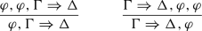
The definition of M-logic is framed after Gentzen’s original system LK (see [8]). All the initial sequents have the form $\varphi \Rightarrow \varphi$, for an arbitrary $\varphi \in Sent_{L_{Ar}}(M)$. The following rules of ML are copied directly from Gentzen’s system:

• Weakening, left and right (W-left and W-right):

  

• Exchange, left and right (E-left and E-right):

  

• Contraction, left and right (C-left and C-right):

  

• Cut:

  

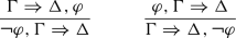
• $\lnot$-left and $\lnot$-right:

  

• $\wedge$-left and $\wedge$-right (for arbitrary sentences $\theta$ and $\chi$ such that one of them is $\varphi$):

  

• $\vee$-left and $\vee$-right (for arbitrary sentences $\theta$ and $\chi$ such that one of them is $\varphi$):

  

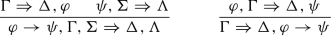
• $\rightarrow$-left and $\rightarrow$-right:

  

In addition, M-logic has the following rules of inference:

• The truth rule for literals (Tr-lit). Let $\varphi$ be of the form $t = s$ with $M \models val(t)= val(s)$ or of the form $t \ne s$ with $M \models val(t) \ne val(s)$:

  

• The M-rule, left and right (M-left, M-right):

  

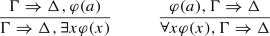
• $\exists$-right and $\forall$-left:

  

Occasionally we will employ Gentzen’s terminology, classifying rules as ‘structural’ or ‘logical’. A logical rule always introduces a logical symbol (for example, the M-rules are logical, since they introduce quantifiers); all the other rules will be referred to as ‘structural’.¹⁸ For a logical rule, the phrase ‘principal formula’ denotes the formula in the lower sequent containing the newly introduced logical symbol (thus, for example, the implication $\varphi \rightarrow \psi$ appearing as the first formula on the left in the lower sequent of the rule $\rightarrow$-left is the principal formula of this rule). For a logical rule, the phrase ‘active formula’ refers to the formula(s) in the upper sequent(s) used in the derivation of the principal formula (thus, for example, in the rule M-right every formula of the form $\varphi (a)$ appearing as the last element in the succedent of one of the upper sequents is to be classified as active).

Proofs in ML are (possibly infinite) trees of finite height, where the height of a proof is defined (as usual) as the length of the maximal path. By definition, trees with no maximal finite path do not qualify as proofs in ML. Note that this is a minor difference between our construction and the one of KKL, who work without such a finiteness restriction. One consequence of this difference is that KKL need to employ the assumption that M is recursively saturated in the consistency proof of their version of M-logic. Indeed, for recursively saturated models the distinction between two systems of M-logic (with and without the finite height restriction) does not correspond to any real difference, namely, it transpires that if M is recursively saturated, then sentences provable in M-logic with no restriction on the height of proofs will always have proofs of finite height.¹⁹ The effect of restricting the heights of proofs is that we will not need the recursive saturation assumption in our consistency proof (the assumption will be employed only to guarantee the transition from the consistent M-logic to the truth class, see Lemma 7 and its proof). Another effect is the overall simplification of the proof, with the point being that in the construction of a truth class we simply do not need to analyze the relation between the two versions of M-logic.²⁰

Observe that in ML, the infinitary rules M-left and M-right replace the original rules $\exists$-left and $\forall$-right of Gentzen.²¹ It should be also emphasized that in all the quantifier rules of ML we employ numerals. Thus, for example, in order to apply $\exists$-right, we need a sentence $\varphi (a)$ where a is a numeral. In contrast, in Gentzen’s original system the rule $\exists$-right would permit us to derive $\Gamma \Rightarrow \Delta , \exists x \varphi (x)$ from $\Gamma \Rightarrow \Delta , \varphi (t)$ for an arbitrary term t, not necessarily a numeral. The effect of this modification of Gentzen’s system is that the truth class which we construct can contain term pathologies. Thus, in a model (M, T) of $CT^-$ which we eventually obtain there can exist a nonstandard formula $\varphi (x)$ such that for some term t, $\varphi (t)$ belongs to T (so that, loosely speaking, the model thinks that $\varphi (t)$ is true), while the sentence $\lnot \exists x \varphi (x)$ also belongs to T. In this way we obtain a disconcerting effect: the model thinks that $\lnot \exists x \varphi (x)$ is true even though it considers as true some term instantiation of $\varphi (x)$.²² (This will happen if all the numerical instantiations of $\varphi (x)$ are seen as false by the model, that is, if for all numerals a, the sentence $\lnot \varphi (a)$ belongs to T.) However, (M, T) can still be a model of $CT^-$, since the quantifier axioms of $CT^-$ only employ numerals.

The expression ‘M-logic’ is a bit of a misnomer, since it is clearly not a system of pure logic for sentences in the sense of M. The extralogical intrusions are not just the infinitary rules (the M-rules given above). In addition, thanks to the (Tr-lit) rule, the system contains the means permitting it to recognize the truth of literals, thus going beyond pure logic also in this respect. We write ‘$ML \vdash \varphi$’ as an abbreviation of ‘$ML \vdash \Rightarrow \varphi$’ (in other words, ‘$ML \vdash \varphi$’ means that M-logic proves the sequent whose antecedent is empty and the succedent contains just $\varphi$). Now, if $\varphi$ is a true literal (that is, if $\varphi$ is of the form ‘$t = s$’ and $M \models val(t)= val(s)$ or $\varphi$ is of the form ‘$t \ne s$’ with $M \models val(t) \ne val(s)$), then $ML \vdash \varphi$, since the sequent $\Rightarrow \varphi$ can be derived from the initial sequent $\varphi \Rightarrow \varphi$ by (Tr-lit).

The lemma below establishes a connection between M-logic and truth classes.

Lemma 7

Let $M \models I \Delta _0 + \exp$ be countable and recursively saturated. If M-logic is consistent, then M can be expanded to a model of $CT^-$.

We will use the notation ‘$ML \vdash _n S$’ for expressing that the sequent S has a proof in M-logic of height at most n (in short, S is n-provable). For the proof of the lemma, we introduce first the family of unary predicates ‘$Pr_n(S)$’ expressing this relation in the arithmetical language; in other words, ‘$Pr_n(S)$’ will be an arithmetical formula expressing that S is n-provable. Observe that for each rule R of M-logic, the relation ‘S can be obtained by R from n-provable sequents’ can always be expressed by an arithmetical formula, provided that n-provability is arithmetically expressible. Thus, for example, ‘S can be obtained by M-left from n-provable sequents’ can be written down as:

$$\begin{aligned} \exists \Gamma , \Delta , \varphi (x) \big ( S = (\exists x \varphi (x), \Gamma \Rightarrow \Delta ) \wedge \forall a Pr_n(\varphi (a), \Gamma \Rightarrow \Delta ) \big ). \end{aligned}$$

In view of this, we introduce the following definition.

Definition 8

• $Pr_0(S) := S$ is an initial sequent.

• $Pr_{n+1}(S) := Pr_n(S)~\vee \bigvee \nolimits _{R \in ML}(S$ can be obtained by R from n-provable sequents).

By external induction on natural numbers it can be demonstrated that:

Observation 9

$\forall k \in \omega ~\forall S \big [ML \vdash _k S \equiv M \models Pr_k(S) \big ]$

We can now turn to the proof of Lemma 7.

Proof of Lemma 7

Let $\varphi _0, \varphi _1, \ldots$ be an enumeration of the set of $M-$sentences (this is the only place where the countability assumption is used).

We define:

$T_0 = \emptyset$

$$\begin{aligned} T_{n+1} = {\left\{ \begin{array}{ll} T_n \cup \{\varphi _n \} &{} \text {if } ML \nvdash (T_n \rightarrow \lnot \varphi _n) \text { and } \varphi _n\text { is not existential},\\ T_n \cup \{\exists x \psi (x) \} \cup \{\psi (a) \} &{} \text {if } \varphi _n = \exists x \psi (x) \text { and ML } \nvdash (T_n \rightarrow \lnot \varphi _n), \\ &{} \text {}\text { for an } a \in M \text { such that } ML \nvdash (T_n \rightarrow \lnot \psi (a)), \\ T_n \cup \{\lnot \varphi _n \} &{} \text {otherwise. } \end{array}\right. } \end{aligned}$$

The above definition strongly resembles the one typically employed in the proof of Lindenbaum’s lemma. The expression ‘$T_n$’ on the right side of the definition (as in ‘$ML \nvdash (T_n \rightarrow \lnot \varphi _n)$’) stands for the conjunction of all the sentences added on previous levels of the construction.

The difference with Lindenbaum’s construction is that here existential statements are always added to $T_n$ together with the witnessing formulas. In view of this, we need to verify that whenever $ML \nvdash (T_n \rightarrow \lnot \exists x \psi (x))$, there will exist an $a \in M$ such that $ML \nvdash (T_n \rightarrow \lnot \psi (a))$. There is no analogous step in the proof of Lindenbaum’s lemma; this is also the only place in the whole proof where recursive saturation of the model is important.

Thus, assume that $ML \nvdash (T_n \rightarrow \lnot \exists x \psi (x))$. Define:

$$\begin{aligned} p(x) = \{\lnot Pr_k(T_n \rightarrow \lnot \psi (x)): k \in \omega \}. \end{aligned}$$

We observe that p(x) is a type. Otherwise there is a natural number k such that $M \models \forall a Pr_k(T_n \rightarrow \lnot \psi (a))$.²³ Hence for all a, $ML \vdash _k T_n \rightarrow \lnot \psi (a)$. But then by the M-rule and cut, $ML \vdash T_n \rightarrow \lnot \exists x \psi (x)$, which is a contradiction.

Since p(x) is a type, by recursive saturation there is an $a \in M$ which realizes it and we have: $\forall k M \models \lnot Pr_k(T_n \rightarrow \lnot \psi (a))$, hence the sentence $T_n \rightarrow \lnot \psi (a)$ is not provable in M-logic, as required.

Now, define T as $\bigcup \nolimits _{n \in \omega } T_n$. The proof of Lemma 7 is completed by demonstrating that $(M, T) \models CT^-$ provided that M-logic is consistent.

The set T is clearly complete (for every M-sentence $\psi$, either $\psi$ or negation of $\psi$ belongs to T) and it contains a numerical example for every existential statement which belongs to T. In addition, since by assumption M-logic is consistent, there is no $\psi$ such that both $\psi$ and $\lnot \psi$ belongs to T. In this setting, checking that all the axioms of $CT^-$ are true in (M, T) is fairly easy and we consider just one example, namely, the axiom for the existential quantifier. In other words, we verify that

$$\begin{aligned} (M, T) \models \forall v \forall \varphi (x)\big (Sent_{L_{Ar}}(\exists v \varphi (v))\rightarrow (T (\exists v \varphi (v) )\equiv \exists x T ( \varphi ({\dot{x}}))) \big ). \end{aligned}$$

Observe that in the proof of both implications the assumption of the consistency of M-logic will be used.

Assume that $(M, T) \models T (\exists v \varphi (v) )$. Let ‘$\exists v \varphi (v)$’ be $\varphi _n$ (that is, let it be the n-th sentence in our enumeration of M-sentences). Then on the level $n+1$ of the construction, $\varphi _n$ must have been added to $T_n$ together with the witnessing statement $\varphi (a)$ for some numeral a (otherwise the negation of $\varphi _n$ was added, but this is impossible since it would make T inconsistent). Therefore $(M, T) \models \exists x T ( \varphi ({\dot{x}}))$.

For the opposite implication, assume that $(M, T) \models \exists x T ( \varphi ({\dot{x}}))$, then for some $a \in M$, $\varphi (a) \in T$. Assuming for the indirect proof that $\exists v \varphi (v) \notin T$, pick a natural number n such that both $\varphi (a)$ and $\lnot \exists v \varphi (v)$ belong to $T_n$. But then all $T_k$-s for $k \ge n$ are inconsistent in M-logic, meaning that for every $k \ge n$, $ML \vdash T_k \rightarrow \psi$ for every M-sentence $\psi$. In effect T would have to contain a pair of contradictory statements, which is impossible. $\square$

4 Consistency of M-logic

At this stage all that is missing for the proof of Theorem 4 is the argument for the consistency of M-logic. In [14] the consistency of M-logic is proved by the technique of approximations; a detailed argument along the same lines is also presented in [7]. Roughly, the authors define a new language which contains fresh predicate symbols corresponding to formulas in the sense of M (formulas of this new language are said to ‘approximate’ those of L(M)); they introduce also a new logic for this language called ‘template logic’ in Engström’s dissertation. The rest of the proof proceeds then by proving the soundness of template logic and establishing the link between M-logic and template logic.²⁴

We will not employ this formal machinery; we opt instead for a syntactic proof with cut elimination as the main tool.²⁵ Let us start by observing that cut elimination is indeed sufficient for our goal.

Proposition 10

If every sequent provable in M-logic has a cut-free proof, then M-logic is consistent.

Proof

If M-logic is inconsistent, then it proves that $0 = 1$. By cut elimination, take a cut-free proof P of $0=1$. It is easy to observe that every sentence in P has to be either atomic or negated atomic (the reason is that without cut, (Tr-lit) is the only rule that permits us to eliminate sentences in the proof and (Tr-lit) can eliminate literals only.) For an arbitrary occurrence S of a sequent in P, let the level of S in P be defined as the length of maximal path generated by S in P.²⁶ Let $Tr_0(x)$ be the arithmetical truth predicate for atomic sentences and their negations. By external induction on the level of occurrences of sequents in P, it can be demonstrated that for every S in P, if all sentences in the antecedent of S are $Tr_0$, then some sentence in the succedent of S is $Tr_0$.²⁷ This trivially holds for level 0 (that is, for the initial sequents). In the inductive part, observe that any S of level $n+1$ must have been obtained in P from sequents of lower level by weakening, contraction, exchange, (Tr-lit) or by the rules for negation applied to atomic sentences; this is so by assumption that P is cut-free and the application of any other rule would introduce a superfluous logical symbol to the conclusion. In effect, very weak resources are enough to verify that if all sentences in the antedecent of S are $Tr_0$ then some element of the succedent of S is $Tr_0$ (in particular, the argument does not require that the model M satisfies any stronger arithmetical theory than $I \Delta _0 + \exp$).

It immediately follows that $M \models Tr_0(0=1)$, which is impossible. $\square$

The next lemma states that cut can be eliminated in all proofs in ML.

Lemma 11

Let M be an arbitrary model of $I \Delta _0 + \exp$. For every sequent S, if S is provable in ML, then S has a cut-free proof in ML.

It immediately follows that M-logic is consistent for every model $M \models I \Delta _0 + \exp$.²⁸

The aim of the remaining part of the paper is to lead the proof of Lemma 11 to the point at which it can be completed simply by repeating Gentzen’s original argument for cut elimination. It should be emphasized that we are not there yet. Our setting is that of possibly nonstandard sentences (sentences in the sense of M) and this generates an obstacle which first has to be removed.

In order to see the obstacle, let us recap the classical argument. The aim is to show that the system with the following mix rule (which is a generalized version of cut) admits mix elimination:

where $\Sigma$ and $\Delta$ contain $\varphi$ (the mix formula); $\Sigma ^*$ and $\Delta ^*$ differ from $\Sigma$ and $\Delta$ only in that they do not contain any occurrence of $\varphi$. Since mix and cut produce equivalent proof systems, mix elimination gives us the desired result.

In the next stage it is demonstrated that mix can be eliminated from any proof which contains only a single application of the mix rule in the last step. This is done by double induction on the degree of proofs (main induction) and on the rank of proofs (subinduction). For proofs with mix used only in the last step, we define:

• The left rank of the proof is the largest number of consecutive sequents in a path starting with the left-hand upper sequent of the mix and such that every sequent in the path contains the mix formula in the succedent.

• The right rank of the proof is the largest number of consecutive sequents in a path starting with the right-hand upper sequent of the mix and such that every sequent in the path contains the mix formula in the antecedent.

• The rank of the proof is the left rank of the proof + the right rank of the proof.

• The degree of the proof is the syntactic complexity of the mix formula.

After this is done, it follows that mix can be eliminated from an arbitrary proof (not just from proofs which contain only a single application of the mix rule in the last step). Namely, given an arbitrary proof P, we can eliminate all the applications of mix stage by stage, by considering subproofs of P which contain mix only in the last step.

When applying this strategy to the case of M-logic, one immediate difference is that in the final part of the reasoning (the one in which mix is eliminated from an arbitrary proof) we have to make sure that the height of the mix-free proof remains finite.²⁹ As for the earlier parts, there is no problem in our setting with induction on the rank of proofs, since both the left and the right rank of the proof in ML will always be a (standard) natural number, restricted by the height of the proof. However, the induction on the degree of proofs in ML is quite problematic. Since the mix formula might be a non-standard element of the model M, its syntactic complexity might be a non-standard number. Arguing externally by induction on non-standard numbers is clearly an invalid move and this is the main obstacle complicating the situation.

Our remedy is to replace the general notion of a degree with a notion relativized to a proof. Assume that we are given a proof P with mix applied only in the last step, that eliminates the (possibly non-standard) mix formula $\varphi$. The guiding intuition to be formalized below is that in the mix-elimination proof the syntactic shape of $\varphi$ matters only comparatively. For example, $\varphi$ might have the form $\lnot \psi$. The intuition is that this will matter only provided that $\psi$ itself (without negation) appears in P; otherwise in the context of a mix-elimination proof $\varphi$ might just as well be treated as a formula of syntactic complexity 0, even if it is non-standard. The underlying reason is that in a mix-elimination proof the notion of a degree of a mix formula $\varphi$ is used only in analysing the case of $\varphi$ being obtained in the proof by a logical rule (thus, in our example, $\varphi$ would be obtained by one of the rules for negation, which means that $\psi$ itself must appear in the proof).

Our objective is to make these ideas precise. In what follows the word ‘sequence’ should always be interpreted externally; in other words, sequences are finite or infinite objects in the real world, not necessarily elements of M. The length of a finite sequence $a = (a_0 \ldots a_k)$ is the number of its elements, that is, $lh(a) = k+1$. For an infinite sequence a we define lh(a) as $\omega$.

Definition 12

Let $\circ$ be an arbitrary binary connective and let $Q \in \{\exists , \forall \}$. We define:

• $x \vartriangleleft y$ (‘x is a direct subsentence of y’) is an abbreviation of the following arithmetical formula:

  $$\begin{aligned}&Sent_{L_{Ar}}(x) \wedge Sent_{L_{Ar}}(y) \wedge \\&\quad \Big ( \exists \psi \in Sent_{L_{Ar}}(y = \lnot \psi \wedge x = \psi ) \\&\quad \vee \exists \varphi , \psi \in Sent_{L_{Ar}}(y = (\varphi \circ \psi ) \wedge x = \varphi \vee x = \varphi ) \\&\quad \vee \exists \theta (x) \in Fm_{L_{Ar}} \exists a \exists v \in Var(y = (Qv \theta (v)) \wedge x = (\theta (a))) \Big ). \end{aligned}$$

• Let $\varphi \in Sent_{L_{Ar}}(M)$. We say that s is a $\vartriangleleft$-sequence for $\varphi$ iff $s_0 = \varphi$ and for every k such that $k+1 < lh(s),~s_{k+1} \vartriangleleft s_k$.

The notion of a degree can now be defined in the following way.

Definition 13

Let P be an arbitrary proof in ML with mix used only in the last step. Let $\varphi$ be the mix formula in P. We define:

• $d(\varphi , P)$ (the degree of $\varphi$ in P) $= sup\{lh(s): s$ is a $\vartriangleleft$-sequence for $\varphi$ such that for every $k < lh(s)~ s_k \in P \}$.

• d(P) (the degree of P) is defined as $d(\varphi , P)$.

The expression ‘$s_k \in P$’ means that the sentence occupying the k-th place in the sequence s appears in some sequent in the proof P. In effect, given a proof P with a mix formula $\varphi$, its degree is identified with the maximal length of a $\vartriangleleft$-sequence generated by $\varphi$ and containing just the sentences used anywhere in P (not necessarily on a single path in P). The actual length of this sequence is left open by the definition; in particular, it is not decided whether the relevant sequence is finite or not. Nevertheless, we are going to demonstrate that proofs with mix used only in the last step always have finite degrees.³⁰

In order to prove this finiteness property, we introduce first the function str(x) (‘the structure of a formula x’). Let the letter p be a new symbol, which will be treated as a propositional variable. Intuitively, given an arithmetical formula $\varphi$, the function str produces a formula of the language with the new symbol which is exactly like $\varphi$, except that the letter ‘p’ is substituted for all occurrences of atomic formulas in $\varphi$.³¹ The function str can be defined by the following arithmetical condition.

Definition 14

$str(x) = y$ iff there are sequences s and $s'$ and a number $k+1$ such that:

• 1. $lh(s) = k+1$ and $lh(s') = k+1$,

• 2. s is a syntactic construction of x (hence $s_k = x$),³²

• 3. $s_{k}' = y$,

• 4. for every $l < k+1$:

  • if $s_l$ has the form $t=s$, then $s_{l}'$ is p,

  • if for some $j < l$, $s_l$ has the form $\lnot s_j$, then $s_{l}'$ has the form $\lnot s_{j}'$,

  • if for some $i, j < l$, $s_l$ has the form $s_i \circ s_j$, then $s_{l}'$ has the form $s_{i}' \circ s_{j}'$,

  • if for some $j < l$, $s_l$ has the form $Qv s_j$, then $s_{l}'$ has the form $Qv s_{j}'$.

Let us extend the arithmetical language by the new unary function symbol $2^x$ for the x-th power of two. Let $\Delta _0(\exp )$ be the class of bounded formulas in the extended language, with new terms functioning as possible bounds (so that, for example, the quantifier $\forall x < 2^y$ counts as bounded). Define $I\Delta _0(\exp )$ as the theory extending Robinson’s arithmetic with appropriate axioms for exponentiation together with the induction schema for all $\Delta _0(\exp )$ formulas.³³ Since it is known that $I\Delta _0(\exp )$ and $I \Delta _0 + \exp$ are equivalent theories,³⁴ the observations to be made below in terms of $I\Delta _0(\exp )$ apply automatically to $I \Delta _0 + \exp$ as well.

Note that given the assumption of binary coding, the expression ‘$str(x) = y$’ can be written down as a $\Delta _0(\exp )$ formula. Let us denote by |x| the length of the binary expansion of x. The quantifier for the lengths of sequences s and $s'$ from Definition 14 can be bounded by $|\varphi | \cdot |\varphi |$; the codes of these sequences will be bounded by $2^{|\varphi | \cdot |\varphi |}$. In effect, the totality of str can be proved already in $I\Delta _0 + \exp$.

Abbreviate $str(\varphi ) = str(\psi )$ as $\varphi \sim \psi$. Let $compl(\varphi )$ be the number of connectives and quantifiers in $\varphi$; we assume that ‘$compl(x) = y$’ is a $\Delta _0(\exp )$ formula. We now observe that a formula which appears at some stage in a $\vartriangleleft$-sequence will always have a larger syntactic complexity than formulas appearing later in this sequence; moreover, sameness of structure implies the same number of logical symbols. This is the content of the proposition below.

Proposition 15

• (a) Let $\varphi$ be an arbitrary (possibly nonstandard) arithmetical sentence and let s be an arbitrary $\vartriangleleft$-sequence generated by $\varphi$. Then for every $\psi \in s$, if $\psi$ is not the first element of s (that is, if $\psi \ne \varphi$), then $M \models compl(\psi ) < compl(\varphi )$.

• (b) $M \models \forall \varphi , \psi \big (\varphi \sim \psi \rightarrow compl(\varphi ) = compl(\psi ) \big )$.

Proof

For the proof of Proposition 15(a), given a $\vartriangleleft$-sequence generated by $\varphi$ denote by $s_n$ (for an arbitrary number n smaller than the length of s) the n-th element of s.³⁵ By external induction we demonstrate that:

$$\begin{aligned} \forall k< lh(s) \big ( k > 0 \rightarrow M \models compl(s_k) < compl(\varphi ) \big ). \end{aligned}$$

In the proof of Proposition 15(b) we work with the assumption that $M \models \varphi \sim \psi$. The conclusion that $M \models compl(\varphi ) = compl(\psi )$ follows then directly from the fact that for an arbitrary $\chi$, the number of connectives and quantifiers in $\chi$ is the same as the number of connectives and quantifiers in $str(\chi )$, i.e., $M \models \forall \chi ~compl(\chi ) = compl(str(\chi ))$. This can be established in $I\Delta _0(\exp )$ by $\Delta _0(\exp )$ induction on the length of sequences a, b, c, d such that:

• $a = (\chi _0 \ldots \chi _k)$ is a syntactic construction of $\chi$,

• $b = (b_0 \ldots b_k)$ is a calculation of complexity of elements of a (in other words, for $l \le k$, $\chi _l$ has $b_l$ connectives and quantifiers)

• $c = (\chi ^p_0 \ldots \chi ^p_k)$ is a syntactic construction of $str(\chi )$,

• $d = (d_0 \ldots d_k)$ is a calculation of complexity of elements of c

with the final effect being that sequences b and d are identical, hence the complexity of $\chi$ (given by $b_k$) is the same as the complexity of $str(\chi )$ (given by $d_k$). $\square$

The key property of the equivalence relation $\sim$ is encapsulated in the following corollary to Proposition 15.

Corollary 16

Let $Z \subseteq Sent_{L_{Ar}}(M)$. For every s, if s is a $\vartriangleleft$-sequence with elements from Z, then $lh(s) \le card\big ( \{[\varphi ]_{\sim }: \varphi \in Z \}\big )$, where $[\varphi ]_{\sim }$ is the class of sentences $\psi$ from Z such that $\varphi \sim \psi$.

Proof

Let s be a $\vartriangleleft$-sequence with elements from Z. It is enough to observe that for no $\varphi$, $\psi \in s$ we will have: $\varphi \sim \psi$ (in effect, no two different elements of s belong to the same equivalence class of the $\sim$ relation, hence the length of s is not greater than the number of equivalence classes). Fix $\varphi$ and $\psi \in s$ and assume (without loss of generality) that $\varphi$ precedes $\psi$ in s. Let $s'$ be the sequence obtained from s by removing all sentences preceding $\varphi$. Then $s'$ is a $\vartriangleleft$-sequence generated by $\varphi$. By Proposition 15(a) we obtain: $compl(\psi ) < compl(\varphi )$ and hence by Proposition 15(b) not $\varphi \sim \psi$. $\square$

We are now ready to demonstrate that proofs with mix used only in the last step always have finite degrees.

Lemma 17

Let P be an arbitrary proof in ML with mix used only in the last step. Then d(P) is a natural number (in other words, it is never $\omega$).

Proof

Fix a proof P in ML which contains mix only in the last step. Let Z be the set of all sentences which appear in P. We demonstrate that $\{[\varphi ]_{\sim }: \varphi \in Z \}$ is finite, which by Corollary 16 guarantees the conclusion of Lemma 17.

For an arbitrary sequent S in P, let l(S) (the level of S) be the length of the path leading from S to the end sequent of P. We denote by $S_i$ the set of all sequents in P whose level is not greater than i. Let $Sent_i$ be defined as the set of all sentences which appear in some element of $S_i$. Let k be the height of P. The task is to show that:

$$\begin{aligned} \forall i \le k \{[\varphi ]_{\sim }: \varphi \in Sent_i \} \hbox {is finite}. \end{aligned}$$

This will end the proof, since $Sent_k = Z$.

We proceed by induction. For $i=0$ the conclusion is trivial, as $Sent_0$ itself is finite ($Sent_0$ is the set of sentences which appear in the end sequent of P). Now, assuming that $\{[\varphi ]_{\sim }: \varphi \in Sent_i \}$ is finite, we claim that $\{[\varphi ]_{\sim }: \varphi \in Sent_{i+1} \}$ is also finite.

Observe that $Sent_{i+1}$ can contain more sentences than $Sent_{i}$ only provided that some sequent of the level i is obtained in P either by mix or by (Tr-lit) or by a logical rule (other structural rules do not generate any new sentences on level $i+1$). If some sequent of the level i is obtained in P by mix, then $i = 0$, since by assumption P contains mix only in the last step. Then the conclusion easily follows, since in such a case $Sent_{i+1}$ is finite (it is simply $Sent_0$ together with the mix sentence). In effect, we can now assume that $i \ne 0$, with no sequent of the level i being obtained in P by mix.

Assume that the set $Sent_{i+1} {\setminus } Sent_{i}$ of new sentences at the level $i+1$ is not empty. Then each element of this set is either eliminated by (Tr-lit) in the next stage of the proof or it is an active formula of the logical inference with the principal formula belonging to $Sent_{i}$. Let us note first that all the elements of $Sent_{i+1} {\setminus } Sent_{i}$ which are eliminated by (Tr-lit) fall into just two possible $\sim$-classes (one for atomic sentences and one for their negations). This leaves us with the second case - that of sentences new on the level $i+1$ which are obtained by logical rules. By inductive assumption, all the principal formulas of logical rules belong to finitely many $\sim$-classes. We will demonstrate that in such a case all active formulas also belong to finitely many $\sim$-classes, which will finish the proof.

Let $[\varphi ]_{\sim }$ be a $\sim$-class on $Sent_i$. We claim that there are at most two $\sim$-classes x and y such that for every $\psi \sim \varphi$, if $\psi$ is the principal formula of a logical inference rule which produces in P the sequent S belonging to $S_i$, then every active formula of this inference rules belongs either to x or to y. Let us analyse cases.

• Case 1: $\varphi = \ulcorner \lnot \theta \urcorner$. Define x as $[\theta ]_{\sim }$. Take an arbitrary $\psi \sim \varphi$ such that $\psi$ is the principal formula of a logical inference rule which produces the sequent S. Then $\psi$ has the form $\lnot \gamma$ and the active formula must be $\gamma$. Since $\lnot \gamma \sim \lnot \theta$, we have $\gamma \sim \theta$, therefore $\gamma \in x$.

• Case 2: $\varphi = \ulcorner \chi \circ \theta \urcorner$. Define x as $[\chi ]_{\sim }$ and y as $[\theta ]_{\sim }$. Take an arbitrary $\psi \sim \varphi$ such that $\psi$ is the principal formula of a logical inference rule which produces the sequent S. Then $\psi$ has the form $\chi ' \circ \theta '$ and the active formula must be $\chi '$ or $\theta '$. Since $\chi \sim \chi '$ and $\theta \sim \theta '$, we have: all active formulas belong either to x or to y.

• Case 3: $\varphi = \ulcorner Qv \theta \urcorner$. Define x as $[\theta ]_{\sim }$. Take an arbitrary $\psi \sim \varphi$ such that $\psi$ is the principal formula of a logical inference rule which produces the sequent S. Then $\psi$ has the form $Qv \chi$ and the active formulas must be of the form $\chi (a)$. Since $\chi \sim \theta$ and for every a, $\chi (a) \sim \chi$,³⁶ we have: all active formulas belong to x.

$\square$

In the proof of the cut elimination lemma one more property of degrees of proofs will be important. In what follows we use the notation Sent(P) for the set of all sentences which appear in a proof P.

Proposition 18

Let $\varphi$ and $\psi$ be M-sentences such that $\psi \vartriangleleft \varphi$. Let P and $P'$ be proofs in M-logic such that:

• Both P and $P'$ contain mix only in the last step.

• The mix formula in P is $\varphi$.

• The mix formula in $P'$ is $\psi$.

• $Sent(P') \subseteq Sent(P)$.

Then $d(P') < d(P)$.

Proof

Since the degree of a proof has been defined as the maximal length of a $\vartriangleleft$-sequence of sentences belonging to the proof generated by the mix formula, let $(\psi , \theta _0 \ldots \theta _k)$ be a maximal such sequence for $P'$. Since $Sent(P') \subseteq Sent(P)$, it is easy to observe that the sequence $(\varphi , \psi , \theta _0 \ldots \theta _k)$ is a a $\vartriangleleft$-sequence of sentences belonging to P generated by $\varphi$. Hence, $d(P') < d(P)$. $\square$

In effect, Definition 13, Lemma 17 and Proposition 18 give us the notion of a degree such that degrees of proofs (with mix used only in the last step) are always standard natural numbers. Hence, induction on the degree of such proofs can be applied and the way to proving cut elimination theorem for ML is now open.

I will not present the whole cut elimination proof, since it is mostly a repetition of Gentzen’s reasoning. Instead, I will mostly restrict myself to discussing the cases of the new rules (the ones not present in the original Gentzen’s system).

Proof of Lemma 11

(Outline and chosen cases). It is demonstrated that: (1) mix can be eliminated from any proof which contains only a single application of the mix rule in the last step, (2) given a proof P with mix only in the last step, the new mix-free proof will employ only sentences used in P, (3) the height of the new mix-free proof $P'$ is determined by the height of the initial proof P. Let us assume (main induction) that mix can be eliminated in this way in every proof of degree $< n$. Let us also assume (subinduction) that mix can be eliminated in this way in every proof of a degree n but with rank $< k$. Our task is to show that mix can be eliminated in this way in proofs of degree n and rank k.

The proof starts with the case of $k =2$ (the lowest possible rank) and proceeds by analysing subcases. Here we analyse only two subcases, with the first one corresponding to a rule of ML absent in LK.³⁷ Namely, let us assume for a start that the mix formula $\forall x \varphi (x)$³⁸ is obtained in P by a logical rule in both the succedent of the left-hand upper sequent of the mix and in the antecedent of the right-hand upper sequent of the mix. Then the last stage of the proof runs as follows:

We can then eliminate mix constructing $P'$ in the following way:

Here the observation is that the same end sequent can be obtained by applying mix to the formula $\varphi (c)$; in effect, we build a proof $P'$ of $\Gamma , \Sigma ^* \Rightarrow \Delta ^*, \Lambda$ which contains mix only in the last step and whose degree is smaller than that of P (the last property follows by Proposition 18, since $Sent(P') \subseteq Sent(P)$). Hence, applying the inductive assumption we conclude that mix in $P'$ can be eliminated without introducing any new sentences absent from $P'$. The final modifications (weakening and exchanges) leading to the end sequent $\Gamma , \Sigma \Rightarrow \Delta , \Lambda$ also do not involve adding to the proof any new formulas (in general: in the present setting new proofs without mix are produced from sentences belonging to the initial proof P). Moreover, the number of weakenings/exchanges to be performed can be showed to depend on the lengths (i.e., number of elements) of sequences $\Gamma , \Sigma$ and $\Delta , \Lambda$, which in turn depend on the height of the initial proof.³⁹ In effect, the height of the mix-free proof will be bounded by a function taking the height of the initial proof as an argument.

The second case we consider is that of the mix formula $\varphi \rightarrow \psi$.⁴⁰ Then the last stage of the proof runs as follows:

We can then transform it into a proof with the following final stage:

Admittedly, at the moment our proof contains two mixes; however, the point is that we can eliminate them one by one. In the first stage by the inductive hypothesis we eliminate mix from the proof of $\varphi , \Gamma , \Sigma _1^* \Rightarrow \Delta ^*, \Delta _1$ (this proof contains mix only in the last step). After this is done, we obtain the proof of $\Sigma , \Gamma ^*, \Sigma _1^{**} \Rightarrow \Lambda ^*, \Delta ^*, \Lambda _1$ containing mix only in the last step, which again can be eliminated by the inductive hypothesis. Note that for this to work, we need the information that at each stage, eliminating mix from a proof P produces a proof $P'$ such that $Sent(P') \subseteq Sent(P)$ (mix elimination introduces no new sentences, cf. Proposition 18), as this guarantees that in both cases the degrees of our mixes fall within the main inductive hypothesis.

When $k >2$, we have in addition the case of (Tr-lit) to analyse. Thus, in the last stage (Tr-lit) could be used to obtain the right-hand upper sequent of the mix. In effect, the last stage of the proof might run as follows:

If $\varphi$ is the mix formula, we can omit (Tr-lit) and use the mix rule instead:

If the mix formula is not $\varphi$, we can build the following proof:

Since in both cases the new proof has lower rank than k (we moved the mix up the derivation), the inductive hypothesis applies and the mix rule is eliminable. The case of (Tr-lit) being used to obtain the left-hand upper sequent of the mix is very similar. $\Box$

With the proof of Lemma 11, the construction of a truth class in a recursively saturated model of $I \Delta _0 + \exp$ has been completed.

We leave as open several natural questions concerning the possibility of applying the present technique in conservativity proofs of extensions of $CT^-$ (that is, of $CT^-$ with new axioms added). In our framework, adding new axioms to $CT^-$ would enforce a corresponding modification in M-logic, where new rules or new initial sequents will also have to be added. In general, the question then would be whether the addition of these new elements preserves the property of cut eliminability, possibly in some restricted form but still permitting to derive the consistency of the extended version of M-logic.⁴¹

References

Cieśliński, C.: Deflationary truth and pathologies. J. Philos. Log. 39(3), 325–337 (2010)
Cieśliński, C.: The innocence of truth. Dialectica 69(1), 61–85 (2015). https://doi.org/10.1111/1746-8361.12093
Cieśliński, C.: The Epistemic Lightness of Truth, Deflationism and its Logic. Cambridge University Press, Cambridge (2017)
Cieśliński, C.: Satisfaction classes via cut elimination. In: Manuel, A., Khan, M.A. (eds.) Logic and Its Applications. Lecture Notes in Computer Science, vol. 11600, pp. 121–131. Springer, New York (2019)
Enayat, A., Visser, A.: Full satisfaction classes in a general setting (Part 1). Unpublished draft (2012)
Enayat, A., Visser, A.: New construction of satisfaction classes. In: Achourioti, T., Galinon, H., Fujimoto, K., Martínez-Fernández, J. (eds.) Unifying the Philosophy of Truth, pp. 321–335. Springer, New York (2015)
Engström, F.: Satisfaction Classes in Nonstandard Models of First Order Arithmetic. Chalmers University of Technology and Göteborg University, Sweden (2002)
Gentzen, G.: Investigations into logical deduction. Am. Philos. Q. 1(4), 288–306 (1964)
Hájek, P., Pudlák, P.: Metamathematics of First-Order Arithmetic. Springer, Berlin (1993)
Horsten, L.: The semantical paradoxes, the neutrality of truth and the neutrality of the minimalist theory of truth. In: Cortois, P. (ed.) The Many Problems of Realism, Volume 3 of Studies in the General Philosophy of Science, pp. 173–187. Tilburg University Press, Tilburg (1995)
Kaye, R.: Models of Peano Arithmetic. Clarendon Press, Oxford (1991)
Ketland, J.: Deflationism and Tarski’s paradise. Mind 108(429), 69–94 (1999)
Kotlarski, H.: Full satisfaction classes: a survey. Notre Dame J. Formal Log. 32(4), 573–579 (1991)
Kotlarski, H., Krajewski, S., Lachlan, A.: Construction of satisfaction classes for nonstandard models. Can. Math. Bull. 24(3), 283–293 (1981)
Kotlarski, H., Ratajczyk, Z.: Inductive full satisfaction classes. Ann. Pure Appl. Log. 47(3), 199–223 (1990)
Krajewski, S.: Non-standard satisfaction classes. In: Lachlan, A., Srebrny, M., Zarach, A. (eds.) Set Theory and Hierarchy Theory. A Memorial Tribute to Andrzej Mostowski. Lecture Notes in Mathematics, vol. 619, pp. 121–144. Springer-Verlag (1977)
Leigh, G.: Conservativity for theories of compositional truth via cut elimination. J. Symb. Log. 80(3), 845–865 (2015)
Łełyk, M.: Nonequivalent axiomatizations of PA and the Tarski Boundary. Unpublished Note (2019)
Robinson, A.: On languages which are based on non-standard arithmetic. Nagoya Math. J. 22, 83–117 (1963)
Smith, S.T.: Nonstandard characterizations of recursive saturation and resplendency. J. Symb. Log. 52, 842–863 (1987)
Tennant, N.: Deflationism and the Gödel phenomena. Mind 111, 551–582 (2002)
Yasugi, M.: Cut elimination theorem for second order arithmetic with the \({\Pi }^{1}_{1}\)-comprehension axiom and the \(\omega \)-rule. J. Math. Soc. Jpn. 22(3), 308–324 (1970)
Acknowledgements
Many thanks to Konrad Zdanowski for helpful comments on some details of the proofs presented in this paper. The author was supported by grant from the National Science Centre in Cracow (NCN), Project Number 2017/27/B/HS1/01830.
Author information
Authors and Affiliations
Corresponding author
Additional information
Publisher's Note
Springer Nature remains neutral with regard to jurisdictional claims in published maps and institutional affiliations.
An extended abstract [4] summarizes the basic ideas presented in this paper. Here we provide both the technical material (proofs) absent in the abstract and a more comprehensive discussion of the motivations and the background of our approach to the semantics of truth theories.
Rights and permissions
Open Access This article is licensed under a Creative Commons Attribution 4.0 International License, which permits use, sharing, adaptation, distribution and reproduction in any medium or format, as long as you give appropriate credit to the original author(s) and the source, provide a link to the Creative Commons licence, and indicate if changes were made. The images or other third party material in this article are included in the article’s Creative Commons licence, unless indicated otherwise in a credit line to the material. If material is not included in the article’s Creative Commons licence and your intended use is not permitted by statutory regulation or exceeds the permitted use, you will need to obtain permission directly from the copyright holder. To view a copy of this licence, visit http://creativecommons.org/licenses/by/4.0/.
About this article
Cite this article
Cieśliński, C. Interpreting the compositional truth predicate in models of arithmetic. Arch. Math. Logic 60, 749–770 (2021). https://doi.org/10.1007/s00153-020-00758-z
Received:
Accepted:
Published:
Issue Date:
DOI: https://doi.org/10.1007/s00153-020-00758-z