Confidence Distributions for FIC Scores


Department of Mathematics, University of Oslo, P.B. 1053, 0316 Oslo, Norway
*
Authors to whom correspondence should be addressed.
Econometrics 2020, 8(3), 27; https://doi.org/10.3390/econometrics8030027
Submission received: 19 December 2019
/
Revised: 21 May 2020
/
Accepted: 12 June 2020
/
Published: 1 July 2020
(This article belongs to the Special Issue Bayesian and Frequentist Model Averaging)
Abstract
:When using the Focused Information Criterion (FIC) for assessing and ranking candidate models with respect to how well they do for a given estimation task, it is customary to produce a so-called FIC plot. This plot has the different point estimates along the y-axis and the root-FIC scores on the x-axis, these being the estimated root-mean-square scores. In this paper we address the estimation uncertainty involved in each of the points of such a FIC plot. This needs careful assessment of each of the estimators from the candidate models, taking also modelling bias into account, along with the relative precision of the associated estimated mean squared error quantities. We use confidence distributions for these tasks. This leads to fruitful CD–FIC plots, helping the statistician to judge to what extent the seemingly best models really are better than other models, etc. These efforts also lead to two further developments. The first is a new tool for model selection, which we call the quantile-FIC, which helps overcome certain difficulties associated with the usual FIC procedures, related to somewhat arbitrary schemes for handling estimated squared biases. A particular case is the median-FIC. The second development is to form model averaged estimators with weights determined by the relative sizes of the median- and quantile-FIC scores.
1. Introduction and Summary
Mrs. Jones is pregnant. She is white, 25 years old, a smoker, and of weight 60 kg before pregnancy. What is the chance that her baby-to-come will have birthweight less than 2.50 kg (which would mean a case of neonatal medical worry)? Figure 1 gives a Focused Information Criterion (FIC) plot, using the Focused Information Criterion to display and rank in this case estimates of this probability, computed via eight logistic regression models, inside the class
where is age, is weight before pregnancy, is an indicator for being a smoker, whereas and are indicators for belonging to certain ethnic groups. The dataset in question comprises 189 mothers and babies, with these five covariates having been recorded (along with yet others; see Claeskens and Hjort (2008, chp. 2) for further discussion). The eight models correspond to pushing the ‘open’ covariates in and out of the logistic regression structure, while are ‘protected’ covariates. The plot shows the point estimates for the 8 different submodels on the vertical axis and root-FIC scores on the horizontal axis. These are estimated risks, i.e., estimates of root-mean- squared-errors. Crucially, the FIC scores do not merely assess the standard deviation of estimators, but also take the potential biases into account, from using smaller models.
Using the FIC ranking, as summarised both in the FIC table given in Table 1 and the FIC plot, therefore, we learn that submodels 000 and 010 are the best (where, e.g., ‘010’ indicates the model with on board but without and , etc.), associated with point estimates 0.282 and 0.259, whereas submodels 100 and 011 appear to be the worst, with rather less precise point estimates 0.368 and 0.226. Again, ‘best’ and ‘worst’ means as gauged by precision of these 8 estimates of the same quantity. Importantly, the FIC machinery, as briefly explained here, with more details in later sections, can be used for each new woman, with different ‘best models’ for different strata of women, and it may be used for handling different and even complicated focus parameters. In particular, if Mrs. Jones had not been a smoker, so that her would rather have been a , we may re-run our programmes to produce a FIC table and a FIC plot for her, and learn that the submodel ranking is very different. Then 111 and 101 are the best and 001 and 000 the worst; also, the estimates of her having a baby with low birthweight are significantly smaller.
The FIC apparatus, initiated and developed in Claeskens and Hjort (2003), Hjort and Claeskens (2003a), and Claeskens and Hjort (2008), has led to quite a rich literature; see comments at the end of this section. FIC analyses have different forms of output, qua FIC tables (listing the best candidate models, along with estimates and root-FIC scores, perhaps supplemented with more information) and FIC plots. The general setup involves a selected quantity of particular interest, say , called the focus parameter, and various candidate models, say S, leading to a collection of estimators . These carry root-mean-squared-errors , and the root-FIC scores are estimates of these root-risks. The FIC plot displays
as with Figure 1.
The present paper concerns going beyond such FIC plots, investigating the precision of each displayed point. The point estimates carry uncertainty, as do the FIC scores. A more elaborate version of the FIC plot can therefore display the uncertainty involved, in both the vertical and horizontal directions. This aids the statistician in seeing whether good models are ‘clear winners’ or not, and whether the ostensibly best estimates are genuinely more accurate than others. In various concrete examples one also observes that a few candidate models appear to be better than the rest. The methodology of our paper makes it possible to assess to which extent the implied differences in FIC scores are significant. Such insights lead also to model averaging strategies with weights given precisely to the best models for the given estimation purpose.
Our paper proceeds as follows. In Section 2 we give the required mathematical background, involving both the basic notation necessary and the key theorems about joint convergence of classes of candidate model based estimators. These results also drive the development of confidence distributions for FIC scores, in Section 3. These in turn also inspire a new variant for the FIC, which we call the quantile-FIC, where each root mean squared error quantity (rmse) is naturally estimated using an appropriate quantile in the associated confidence distribution. A special case is the median-FIC; details are given in Section 4. Having established such results, Section 5 then involves constructions of median-FIC driven weights for model averaging operations, where we also give a precise large-sample description of the implied model averaging estimators. In Section 6 we address performance and comparison issues, studying relevant aspects of how well different strategies behave, from post-FIC to model averaging estimators. It is in particular seen that the post-median-FIC estimators have certain advantages over post-AIC schemes. More information concerning performance is brought forward in Section 7, via simulation experiments, in four different setups. To display how our new CD–FIC based methods work in a setup with considerably more candidate models at play than with the models used for Mrs. Jones above, a multi-regression Poisson setup is worked through in Section 8, involving abundance of bird species for 73 British and Irish islands. Then we sum up various salient points in our discussion Section 9, and offer a list of concluding remarks, some pointing to further research, in Section 10. In a separate Appendix, Section 11, we give technical details and formulae for required quantities and ingredients for candidate models inside a general regression framework.
We end our introduction section by commenting briefly on other relevant work, first on the FIC front and then on model averaging. Setting up FIC schemes involves finding good approximations to mse quantities, and then constructing estimators for these. This pans out differently in different classes of models, and sometimes requires lengthy separate efforts, depending also on the type of focus parameter. Claeskens and Hjort (2008) cover a broad range of general i.i.d. and regression models, using local neighbourhoods methodology. Later extensions include Claeskens et al. (2007) for time series models, Gueuning and Claeskens (2018) for high-dimensional setups, Hjort and Claeskens (2006) and Hjort (2008) for semiparametric and nonparametric survival regression models, Zhang and Liang (2011) for generalised additive models, Zhang et al. (2012) for tobit models, Ko et al. (2019) for copulae with two-stage estimation methods. Recent methodological extensions and advances also include setups centred on a fixed wide model, with large-sample approximations not depending on the local asymptotics methods; see Claeskens et al. (2019); Jullum and Hjort (2017, 2019), along with Cunen et al. (2020) for linear mixed models. There is a growing list of application domains where FIC is finding practical and context-relevant use, such as finance and economics (Behl et al. 2012; Brownlees and Gallo 2008), peace research and political science (Cunen et al. 2020), sociology (Zhang et al. 2012), marine science (Hermansen et al. 2016), etc. There is similarly a rapidly expanding literature on frequentist model averaging procedures, as partly contrasted with Bayesian versions; perspectives for the latter are summarised in Hoeting et al. (1999). A broad framework for frequentist averaging methods is developed in Claeskens and Hjort (2008); Hjort and Claeskens (2003a), including precise large-sample descriptions for how such schemes actually perform. Wang et al. (2009) give a broad review. In econometrics, Hansen (2007) studies model averaging for least squares procedures, and Magnus et al. (2009) compare frequentist and Bayesian averaging methods. Optimal weights are studied in Liang et al. (2011). The book chapter Chan et al. (2020) discusses optimal averaging schemes for forecasting, touching also the phenomenon that simpler weighting methods sometimes perform better than those involving extra layers of estimation to get closer to envisaged optimal weights.
2. Basic Setup and the FIC
In this section we give the basic theoretical background and main results behind the FIC plot (1). It is convenient to describe the i.i.d. setup first, and to describe a canonical limit experiment with the required basic quantities. In Section 2.2 we then briefly explain how the apparatus can be extended also to general regression models, where it also turns out that the limit experiment is of exactly the same type, only with somewhat more complex mechanisms lying behind the key ingredients. Technical details and explicit formulae for such general regression models, valid also beyond the realm of say generalised linear models, are provided in Section 11. The key results described in this section are behind the FIC plots and the FIC tables, such as Figure 1 and Table 1, and will also be used in later sections to derive confidence distributions for risks.
2.1. The I.I.D. Setup
Suppose we have independent and identically distributed observations, say . A collection of candidate models is examined, ranging from a well-defined narrow model, parametrised as with of dimension p, to a wide model, parametrised as , with certain extra parameters , signifying model extensions in different directions. The narrow model is assumed to be an inner point in the wider model, in the sense of being equal to for an inner parameter point . There is consequently a total of candidate models, corresponding to setting parameters equal to or not equal to their null values , for . In the regression framework studied below this would typically correspond to taking covariates in and out of the wide model.
Other terms could be considered here, like ‘full model’ for the wide model and ‘null model’ for the narrow model, but we choose to stick to the ‘wide’ and ‘narrow’ labels as these have been used rather consistently in the FIC literature, from Claeskens and Hjort (2003) onwards. Furthermore, the alternative ‘null model’ term would risk being associated with a suggestion that the point of the setup is to test it, against various alternatives, but this is typically not the aim of the model selection and model averaging framework.
Assume now that a parameter is to be estimated, with a clear statistical interpretation across candidate models. It may in particular be expressed as in the wide model. We may then consider different candidate estimators, say based on the submodel S, with S a subset of , corresponding to the model having as a parameter in the model when but with set to their null values for . Carrying out maximum likelihood (ML) estimation in model S means maximising the log-likelihood function , with notation for the collection of with , and similarly for with the complement set. With the ML estimators for submodel S, this leads to a collection of candidate estimators
In particular we have and , with ML estimation carried out in respectively the narrow p-dimensional and the wide -dimensional models.
To understand the behaviour of all these candidate estimators, and to develop theory and methods for comparing them, we now present a ‘master theorem’, from Hjort and Claeskens (2003a), Claeskens and Hjort (2008, chp. 5, 6). We work inside a system of local neighbourhoods, where the real data-generating mechanism underlying our observations is
with some unknown , seen as a local model extension parameter; in particular, the true focus parameter becomes . A few key quantities now need proper definition. We start with the Fisher information matrix J with inverse , defined for the wide model with parameters, but computed at the narrow model, i.e., at . We need to involve their blocks, so
with and of size , etc. The matrix
serves a vital role. So do also
with partial derivatives evaluated at the narrow model, and with these quantities varying from focus parameter to focus parameter. Finally we need to introduce the matrices
Here, is the projection matrix of zeroes and ones, such that , taking to its subset of those with . We have and , the identity matrix, and note that , the number of elements in S.
The master theorems driving much of the FIC and related theory are now as follows. First,
and, secondly,
Here, , for the given above, and and D are independent. This implies that the limit in (6) is normal, and we can read off its bias and variance . The risk or mean squared error for this limit distribution is hence
say, in the usual fashion a sum of a variance part and a squared bias part . With a sparse S, there are many zeros in , leading to small variance but potentially a larger bias; with a bigger subset S, becomes closer to the identity matrix I, yielding bigger variance but a smaller bias.
The essence of the Focused Information Criterion (FIC), developed in Claeskens and Hjort (2003, 2008) and later extended in various directions and to more general contexts and model classes, is to estimate each from the data. This leads to a full ranking of all candidate models, from the best (smallest estimate of risk) to the worst (largest estimates of risk). Briefly, we start by putting up FIC formulae for the limit experiment, where all quantities are known (thanks to consistent estimators for these, see below), but where is not, as we can only rely on the information from (5). Noting that , which also means that using to estimate a squared linear combination parameter means overshooting with expected amount , there are actually two natural versions here, namely
These correspond to the natural unbiased estimator and its truncated-to-zero version for the squared bias. That the first estimator for squared bias is negative means that the event
is taking place, which happens quite frequently if is close to zero, in fact with probability up to , if , but is growing less likely when is moving away from zero.
For actual data one plugs in consistent estimators for the relevant quantities, to be given below, and of (5) for . This leads to FIC scores
Note from (6) that these are estimators of the limiting risk, where has been multiplied with . Most often it is therefore better, regarding reading of tables and interpretation of FIC plots, to transform the above scores to say
We consider the truncated version a good default choice, since it avoids having negative estimates of squared biases, and this choice has indeed been used for Mrs. Jones and her FIC plot in Figure 1 and FIC table in Table 1. The consistent estimators in question are computed as follows. From ML analysis in the wide model, maximising , we compute the normalised Hessian matrix at this ML position, say ,
of size . This is a consistent estimator for J of (3) under the assumed sequence of data-generating mechanisms (2), under mild conditions; see Claeskens and Hjort (2008, chp. 6). Inverting this matrix and reading off its lower right block leads to , consistent for Q. Finally and are defined by plugging in relevant blocks of in (4), along with partial derivatives of , computed at the ML position . There are in fact a few alternatives here, regarding estimation of J and , but these do not affect the basic asymptotics; see Claeskens and Hjort (2008, chp. 6, 7) for further discussion.
2.2. Extension to Regression Models
As demonstrated in (Claeskens and Hjort 2003, 2008) the theory briefly reviewed above for the i.i.d. setup can with the required extra effort be lifted to the framework of regression models. Data are then of the form , with a covariate vector and the response. The natural setup becomes that of a wide regression model with densities , featuring a narrow model parameter of size p and an extra parameter of size q, and where a null value yields the narrow model. Again using as the natural framework of local asymptotics, there are under mild Lindeberg conditions clear limiting normality results for all submodel based estimators, etc., parallelling those of (5)–(7), though involving somewhat more complex notation than for the i.i.d. case when it comes to key quantities . Technical details and formulae are provided in Section 11.
It is however simplest to develop our extended CD–FIC theory for the i.i.d. case, which we make our task below. For each method and result reached below there is a natural extension to the case of regression models. This is illustrated in Section 8 for a class of Poisson regression models applied to a study of bird species abundance. Furthermore, our introductory illustration, involving low birthweights, is an application of the general methodology to logistic regression models.
3. Confidence Distributions for FIC Scores
The FIC scores of (8) are estimators of the quantities (7), defined in the limit experiment where and the other key quantities are known. Similarly, the scores of (10) are estimating the genuine , the root-mse for the estimators . However, the FIC scores carry their own uncertainty, which we address in this section through constructing confidence distributions for the estimated quantities.
As in Section 2 we start working out matters in the clear limit experiment, and then insert consistent estimators when engaged with real data. A brief prelude to explain what will take place is as follows: Suppose a single X is observed from a , and that inference is needed for the parameter . Since is a noncentral chi-squared, with 1 degree of freedom and noncentrality parameter , which we write as , we can build the function
with the cumulative distribution function for the . Here, is the observed value of the random X. The is a cumulative distribution function in , for the observed , with the property that for each , when X comes from the data model , then has the uniform distribution:
In other words, defines an exact confidence distribution (CD), see Hjort and Schweder (2018); Schweder and Hjort (2016), and confidence intervals can be read off from . Note that this CD has a pointmass at zero, , involving the standard chi-squared cumulative . Thus confidence intervals for could very well start at zero. This CD is the optimal one, in this situation, cf. Schweder and Hjort (2016, chp. 6).
Going back to the of (7), write
with
Here, is the limiting variance of . It is smaller with fewer elements in S, and becomes larger with more elements. Furthermore, is the variance of , i.e., of the estimate of the bias . Write for clarity , which has a distribution, with . Since quantities are known, in the limit experiment, the arguments above lead to the CD
It starts at position , the minimal possible value for , with pointmass there of size .
The narrow model, with and , has the smallest , namely , but also the largest , with
On the other side of the spectrum of candidate models, the widest model has , the is the constant with no additional uncertainty, in this framework of the limit experiment, and the is simply a full pointmass 1 at that position.
For a real dataset, we estimate the required quantities consistently, as per Section 2, and with of (5) for D. Translating and transforming also to the real root-mse scale of
we reach the data-based CD
Here, and , and the CD starts with the pointmass at its minimal position . The CD is large-sample correct, in the sense that for any given position in the parameter space, its distribution converges to that of the uniform as sample size increases. Thus defines a confidence interval for , with coverage converging to .
In Figure 2 confidence distributions are displayed for the eight true root-mse values pertaining to the eight submodels in the Mrs. Jones example of our introduction. Clearly, several of the CDs have pointmasses well above zero. Furthermore, displayed in the figure are three root-FIC scores of different type: the already mentioned and , along with the median-FIC which we come to in the next section. The unbiased estimator can for some models be considerably smaller than ; indeed it has the value zero for the narrow model 000. The models with smaller than have negative squared bias estimates, i.e., , then the ratio inside will be smaller than 1, which leads to the corresponding CDs starting with a pointmass higher than .
In our first exposition of the case of Mrs. Jones, Figure 1 gave eight point estimates for the probability of her child-to-come having low birthweight, along with root-FIC scores. From the CDs in Figure 2 we can construct an updated and statistically more informative FIC plot, namely Figure 3, which provides accurate supplementary information regarding how precise these root-FIC scores are. The figure provides confidence intervals for both the root-FIC scores and the focus estimates. In particular, we see that the FIC score for the winning model 000 appears to be very precise, and we may then select this model without many misgivings. The scores of the next best models 010 and 001 appear to be more uncertain, and their intervals indicate that their underlying true rmse values are potentially much larger than what their root-FIC scores indicate.
4. Median-FIC and Quantile-FIC
As briefly pointed to in Section 2, there are often two valid variations on the basic FIC, when it comes to estimating the precise quantities, as in (8) and (9). The first uses the unbiased risk estimator, involving the possibility of having negative estimates for squared biases, whereas these are truncated up to zero for the second version.
Since the most natural way of assessing uncertainty of these risk estimators is via CDs, as in Section 3, with confidence pointmasses at the smallest values, etc., a third version suggests itself, namely the median confidence estimators. Generally, these have unbiasedness properties on the median scale, as opposed to on the expectation scale, and are discussed in Schweder and Hjort (2016, chp. 3, 4). Thus consider the median-FIC,
defined for the limit experiment, via (11), to be viewed as an alternative to and of (8). For actual data, having estimated the required background quantities and also transformed to the scale of , we use the CD of (12), and infer the median-FIC score
See Figure 2 where we display the 0.50 confidence line and read off the corresponding medians.
Considering the limit experiment case (13) first, we know that the CD starts out at the minimal point with the pointmass . If this is already at least , which inspection shows is equivalent to , then the median-FIC is equal to . If that ratio is above 0.6745, however, then the median-FIC is the numerical solution to
viewed as an equation in . Correspondingly, if
for a given dataset, then the median-FIC for is equal to the minimum value , and otherwise one solves numerically with a solution to the right of .
Going back to the limit experiment framework again, with the relative size of the estimated bias versus its uncertainty, we have the following relations between the three different FIC scores. (i) If , then ; (ii) if , then ; (iii) if , then . In particular, it is always the case that . Since the three types of FIC scores are identical for the wide model, the three strategies can be understood as having increasing preference for selecting the wide model. The unbiased-FIC generally gives smaller FIC scores to all models except the wide model, so it will therefore have a smaller probability of selecting the wide. The median-FIC, on the other hand, typically gives larger FIC scores to the competing models, and is then more likely to select the wide model. The truncated-FIC lies somewhere between these two approaches. We will compare the three strategies in more detail in Section 6, where each strategy is studied also in terms of the risk of the estimator which the FIC score selects.
In addition to the median confidence estimator associated with the CDs it is also valuable to consider the more general quantile-FIC, which is
for any given . We learn in Section 6 that quantile values smaller than 0.50 may be beneficial for estimating the squared bias parts when these are small to moderate.
Similarly to our brief comments about the median-FIC score above, we may work out some of the relations between the previously existing FIC scores and the quantile-FIC score. We may for example study the specific choice of . This score, denoted by , will be equal to when . For larger values one needs to find the numerical solution of . Naturally, . Further, if , then , but if , then . The lower-quartile-FIC will thus often be smaller than the previously existing FIC scores, as opposed to the median-FIC which will always be larger or equal, as we saw above. Since all the FIC scores are identical for the wide model, this entails that will exhibit a preference for selecting smaller models. We will come back to these insights in the discussion section.
5. Model Averaging
Our FIC investigations above also invite new and focused model averaging schemes, where the weights attached to the different candidate models are allowed to depend on the specific focus parameter under consideration. Consider model averaging estimators of the general form
with weights depending on of (5), assumed to sum to 1, and with limits . Coupling with
of (6), and utilising the joint limit distribution for the variables involved, a master theorem is reached in Claeskens and Hjort (2008, chp. 7) of the form
This result is generalised to yet larger classes of model averaging strategies, including bagging procedures, in Hjort (2014).
In the present context, a natural averaging estimator is as above, with weights of the form
The master theorem applies, which means we can read off the accurate limit distribution for the median-FIC based model averaging scheme in question. We may also use different tuning parameters for different models, i.e., with weights proportional to , with appropriately selected . A general venue is to use the CDs for each model in order to set such model-specific values. One possibility is to evaluate all the CDs at the estimated rmse value of the widest model and then let
see (12). For the wide model the is a unit point mass at the position , and we take , but for the other models the will have values above 1; see Figure 2. The intuition is that dividing the FIC score with the confidence, evaluated at this specific point, will give higher weights to models where the FIC scores are more certain. This is the method we have employed for Figure 4, for the model averaging scheme there denoted ‘CD–FIC weights’.
There are clearly several other model averaging schemes that may be considered based on the CDs for the FIC scores. For example, one may wish to use only models which have a high probability of having a rmse lower than a certain threshold, and then use a similar weighting scheme as above among the models with scores falling below this threshold. Again our master theorem (17) applies, with a precise description of the large-sample distributions of the ensuing model averaging estimators.
In Figure 4 we present a brief illustration of different model selection and averaging schemes. The figure displays the limiting distribution densities of , from (17), for five different strategies. The densities are produced not by simulating from some given model with a high sample size, but from the exact limit distributions, by drawing from and D. A sharper density around zero indicates that the strategy produces a more precise estimator than the others. The sharpness around zero may be assessed by computing the limiting mse of each , by simply summing the squared draws from the limiting distributions. For this illustration we have used , with submodels, Q equal to the identity matrix, equal to 0.1357, and the set to . The red line represents the scheme where one always chooses the widest model. In that case the focus estimator is unbiased and its distribution is a perfect normal (as we see). The two blue lines are model selection strategies, where a single model is chosen, either using the classic AIC (light blue), or using our new median-FIC score (dark blue). We see that both strategies induce some bias in the final estimator, and that the distribution of is a complicated nonlinear mixture of normals. The two green lines are model averaging strategies. The light green one is the scheme with weights as in (18), with . The dark one is a strategy making use of the confidence distributions for the FIC score, with as in (19).
For this particular position in the parameter space the two model averaging strategies produce the most precise estimators, obtaining limiting root-mse values of about 1.26 and 1.58 for the average of median-FIC and average with CD–FIC weights. The limiting root-mse values for the method selecting the best estimator according to the best median-FIC score or best AIC scores are respectively 1.60 and 1.67. The strategy of always selecting the wide model has a limiting rmse of 1.74, and is thus the least precise strategy among the five for this position in the parameter space.
6. Performance Aspects for the Different Versions of FIC
Our FIC procedures use estimates of root mean squared errors to compare and rank candidate models, and as we have demonstrated also lead to informative FIC plots and CD–FIC plots. There are several issues and aspects regarding performance, including these:
- (a)
- How good is the root-FIC score, as an estimator of the rmse?
- (b)
- How well-working is the implied FIC scheme for finding the underlying best model, e.g., as a function of increasing sample size?
- (c)
- (d)
- How well-working are the (approximate) CDs regarding coverage properties; do confidence intervals of the type contain the true 80% of the time?
We note that themes (b) and (c) are quite related, even though different specialised questions might be posed and worked with to address particularities. Furthermore, in various contexts, theme (c) is what matters.
Methods to be compared are the unbiased , the truncated , the median-FIC , and also its more general variant the for other useful quantiles q. Themes (a), (b), (c), (d) can of course be studied for finite sample sizes, in different setups and with many variations, and indeed these questions addressed in Section 7 below. It is again illuminating to work inside the limit experiment setup of Section 2 and Section 3, however, where complexities are stripped down to the basics. This involves certain known basis parameters and the crucial relative distance parameter estimated via a single . Below we report on relatively brief investigations into themes (a), (c), and return also to (b), (d) in the next section.
6.1. FIC for Estimating MSE
The limiting expressions are of the form , say, as per (7), with and known quantities. The different FIC schemes differ with respect to how the squared bias term is estimated. In the reduced prototype form worked with at the start of Section 3, the comparison boils down to investigating four methods for estimating in the setup with a single . The unbiased and truncated FIC are associated with the estimation schemes and , and both of these uniformly beat the simpler maximum likelihood estimator (which is hence inadmissible, in the decision theoretic sense). The median-FIC corresponds to setting equal to the median of the confidence distribution . Risk functions can now be numerically computed and compared, for the different estimators, yielding say ; the first is incidentally equal to . Figure 5 displays four root-risk functions, i.e., . We learn that the two ‘usual’ FIC based methods, the unbiased and truncated, are rather similar, though the truncated version is uniformly better for this particular task. The quartile-FIC is significantly better for a relatively large window of squared bias values, whereas the median-FIC is better when such values are large.
6.2. Narrow vs. Wide
We now consider a relatively simple setup, where we only wish to choose between two models, the narrow (with p parameters) and the wide (with parameters). The limiting mean squared errors are
from which it also follows that the narrow model is better than the wide in the infinite band . The FIC in effect attempts to use data to see whether is inside this band or not. We have
Thus the unbiased says that the narrow is best if and only if , and a bit of analysis reveals that the truncated in this case is in full agreement. In the limit experiment of this two-models setup, has the estimators and , and the final estimator used is
Here,
This FIC strategy is then to be contrasted with that of the median-FIC. The question is when
where
This means finding when the function crosses 0.50, and a simple investigation shows that prefers the narrow to the wide model if and only if .
The limiting risk functions for the three FIC methods for reaching a final estimator are therefore of the form
using (20), with cut-off value for and , and with for . More generally, the quantile-FIC method of (15) can be seen to have such a cut-off value , which is, e.g., for . The conservative strategy, choosing the wide model regardless of the observed D, corresponds to cut-off value .
Let us also briefly point to the classic AIC method, in this setup. As shown in Claeskens and Hjort (2008, chp. 5, 6), in the limit AIC prefers the narrow over the wide model if and only if . With notation as in Section 2 and Section 3, the limit distribution of the AIC selected estimator becomes
When there is only extra parameter in the wide model, this is the very same as for the two first FIC methods, with cut-off value .
Figure 6 displays root-risk functions for the usual FIC (with , full curve), for the median-FIC (with , dotted curve, low max value), and the quantile-FIC with (with , dotdashed curve, high max value). We see that the median-FIC often wins over the standard FIC, and its maximum risk is considerably lower. More precisely, median-FIC has the lowest risk in the parts of the parameter space where the wide model is truly the best model, but where only has moderately large values, i.e., the parts of the parameter space where the true model is at some moderate distance from the narrow model. This fits well with some of our insights from Section 4, where we saw that median-FIC will select the wide model with a higher probability than ordinary FIC. For moderate values, the median-FIC turns out to balance its submodel selection probabilities well, in the sense of securing relatively small risk for the final estimator. For values farther away from zero all strategies always select the wide model and they therefore have identical risk.
For values closer to zero, in the part of the parameter space where the narrow model is truly more precise than the wide, we see that median-FIC has a higher risk than the other strategies and that quantile-FIC with is the best strategy. Again this is related to our comments in Section 4, with quantile-FIC tending to give lower FIC scores to the non-wide models, compared to the other strategies. In this scenario, this gives a propensity to select the narrow model. This property is advantageous for values around zero, but gives a higher risk for moderately large values.
6.3. Three FIC Schemes with Q = 2
We continue with the somewhat more complex case where we have extra parameters in the wide model, and four submodels under consideration, here denoted by 0, 1, 2, 12. We let be diagonal, in order to have simpler expressions than otherwise. This in particular means that and become independent in the limit. The expressions for the four different candidate models are then
where are considered known parameters, whereas what one can know about is limited to the independent observations and . The FIC scores , , will depend on these known parameters and on , and the associated limiting risks will be functions of ,
for the three different versions of
with the associated indicator functions for where submodels 0, 1, 2, 12 are selected.
We can now compute and compare these risk functions in the two-dimensional space, for each choice of . Since the mse expressions, as well as the risk functions, all have the same term, we disregard that contribution, and in effect set . In Figure 7 we show the results of such an exercise, with and . On the left hand side, we see that for this setup median-FIC gives lower risk than the two other strategies for a relatively large part of the parameter space. The right side shows the ratio between the risk of median-FIC and the best competing strategy. The panels indicate that median-FIC beats the two other strategies for moderate values of both and , but loses when one or both of these quantities are close to zero, and also when both are large in absolute size.
This is consistent with our observations in Section 4; the median-FIC has good performance in the parts of the parameter space where the wide model is truly the best. If quantile-FIC with had been included in this comparison, we would have discovered that beats the other strategies in the areas were the wide model is not the best, particularly in the narrow diagonal band from to .
7. Finite-Sample Performance Evaluations
Complementing the performance analyses of Section 6, in the framework of the limit experiment, we have conducted various investigations of the performance of the FIC scores and of the CDs in finite-sample settings, via simulations. In these experiments we sample data from a known wide model and with a particular choice of focus parameter, for which we then know the true value. We generate a high number of datasets from this model, and compute FIC scores and CDs for each of these. From this we can investigate aspects (a), (b), (c), (d) mentioned in the beginning of the previous section. Do the root-FIC scores succeed in estimating the true rmse? And do the FIC scores provide a correct ranking of the models? Further, we can investigate the coverage properties of our CDs: do the confidence intervals we obtain from the CDs, say the , cover the true rmse values for approximately 80% of the rounds? We will present the results from four different simulation setups: (1) a linear regression model with relatively few candidate models, (2) a linear regression model with many candidate models, (3) a Poisson regression, and (4) a logistic regression.
Our first two illustrations are for datasets of observations from a linear normal model with the structure , with errors being independent from , and with focus parameter of the type . In the first setup we have an intercept parameter protected (so ) and three extra parameters associated with three covariates considered for ex- or inclusion (). The narrow model has only the intercept parameter, and the wide model has the intercept term and all three covariates. The other candidate models correspond to including or excluding the three covariates. We have used , , and residual standard deviation . The covariates are drawn from a multivariate normal distribution with zero means, unit variances, and intercorrelations chosen to be , , . The focus parameter is , with and . The red line in the left panel of Figure 8 indicates the true rmse values for the eight models. The grey crosses are the root-median-FIC scores evaluated in datasets. The black dashed line gives the average scores from these datasets. In the right panel, we see the realised coverage of the computed 80% confidence intervals. Note that the realised coverage for the wide model (here ) will always be zero as our framework does not yield confidence intervals for the widest model, but only a point estimate, by construction. Table 2 reports the percentage of rounds where each model has the lowest FIC score (i.e., the winning model). In this setup, model 5 had the lowest true rmse (as we see in the figure), and the wide model had the second lowest rmse.
In our second setup, we investigated a linear normal model with a higher number of covariates, and a much higher number of candidate models. Again we have and an intercept parameter protected (so ), but this time we have ten extra parameters considered for ex- or inclusion (). There are then 1024 candidate models. We have used , , and residual standard deviation . The covariates are drawn from a multivariate normal distribution with zero means, variances between 0.9 and 2.2, and correlations ranging from to . Again the focus parameter is of the form , with and . For the sake of presentation, we have chosen to present the results for 100 among the 1024 candidate models, see Figure 9. The first model is the narrow model, the last is the wide, and the remaining are a random selection among the candidate models. Figure 9 presents the same type of results as Figure 8, but because of the high number of candidate models we have not include this setup in Table 2.
Naturally, the size of the residual standard deviation is a crucial importance here, as seen also via the exact Formula (21). For small , the bias part dominates, and the is smallest for wider and more elaborate models; for larger , the variance part dominates, with being smallest for simpler models with fewer regression terms. These aspects are also picked up by the FIC. It also follows from our analyses of the CD approximations that the confidence coverage property is more precise for smaller than for bigger .
Our third setup is a Poisson regression model where we simulate datasets of the same size and with the same covariates as in our application in Section 8. Here, , , , giving 48 submodels; see further details in the section mentioned. We also use the same focus parameter as we describe there, and simulate data from the fitted wide model, corresponding to parameter values , . In Figure 10, we present the same type of results as for the previous setups, but here we have used instead of median-FIC. With this criterion the truly best model was correctly identified in 63.5% of the rounds.
In our fourth setup we simulated binary observations from a logistic regression model of the same form as in Section 1, but with and . We let , . Our focus parameter is the probability of an event for a certain vector of covariates, and . The results are presented in Figure 11 and Table 2. In this setup, the truly best model was , closely followed by .
From the left panels in each of the four figures in this section, we see that average root-FIC scores are generally close to the true rmse values. The FIC score selects the truly best model, in terms of mse, for most of the rounds, but not always. The ability to select the best model depends on the estimation quality of the FIC scores, but also on how close, or different, the rmse values of the models really are. In the first setup, is the truly best model, but the wide model is often preferred by the FIC score. This might appear disappointing, but in fact these two models have almost identical performance (the red line in Figure 8). Similarly, in the logistic regression setup the two best models had very similar performance and were often selected by the FIC machinery. In the Poisson regression setup the correct model was identified surprisingly often given the relatively high number of candidate models.
The right panels in the four figures are possibly even more interesting, since the main contribution in this paper are the CDs for the rmse. The realised coverage of the 80% confidence intervals is generally close to 80%, but for some candidate models it is considerably lower than the nominal level. First, as mentioned already, we do not get confidence intervals for the wide model in this framework, only an unbiased point estimate, so its realised coverage will always be zero. For other candidate models than the wide, the under-coverage phenomenon happens for candidate models which consistently produce very steep CDs. These are candidate models which have a small estimated bias, and also a small variance-term related to the estimation of the bias ( in our terminology). Reassuringly, for all the cases we have investigated, the candidate models with under-coverage consistently have very small spread in their FIC scores (note for instance in Figure 11). These candidate models thus should really get narrow confidence intervals, but these happen to become too narrow. Ultimately, the observed under-coverage is a consequence of our CDs being constructed based on the approximation to the limit experiment, and there is therefore a layer of uncertainty not accounted for in our construction; see the discussion in Section 9.
8. Illustration: Birds on 73 British and Irish Islands
Reed (1981) analysed the abundance of landbirds on 73 British and Irish islands. In the dataset, characteristics of each island were recorded: the distance from mainland (), the log area (), the number of different habitats (), an indicator of whether the island is Irish or British (), latitude (), and longitude (). As the notation indicates, we take as protected covariates, to be included in all candidate models, whereas are open. Based on general ecological theory and study of similar questions we also include two potential interaction terms, viz. and . Of the candidate models, corresponding to inclusion and exclusion of , we only allow the interaction term in a model if is also inside; this leaves us with candidate models below.
Suppose we take an interest in predicting the number of species on the Irish island of Cape Clear. In Reed’s dataset we have the following information about this island: it is located at 6.44 km from the mainland, at 51.26 degrees north and degrees east, with an area of 639.11 hectares. At the time of study it had 20 different habitats (), and 40 different bird species () were observed. Assume that we know that the number of habitats has decreased to 15 – which model gives the most precise estimate of the current number of species?
As the required wide model we choose the Poisson regression model, with , where
The wide model thus has nine parameters to estimate, while the smallest, narrow one only has three. We conduct our FIC analysis, and using our confidence distribution apparatus we obtain our extended FIC plot with uncertainty bands in Figure 12. Some models indicate a clear improvement compared to the wide model, with very low uncertainty around their FIC scores. The winning model is similar to the narrow model, but includes the habitat covariate. Most of the models with low FIC scores contain this covariate, and one or both interaction terms or the longitude covariate (Cape Clear lies quite far west compared to most of the islands in the dataset). The predicted number of species on Cape Clear among the favoured models is around 29, a decrease from the 40 species in the dataset.
The point to convey with this application is also that any other focused statistical question of interest can be worked with in the same fashion. Natural focus parameters could be the probability that y falls below a threshold , given a set of present or envisaged island characteristics, or the mean function itself, for a given set of covariate combinations. For each such focused question, a FIC analysis can be run, leading to FIC plots and finessed CD–FIC plots as in Figure 12, perhaps each time with a new model ranking and a new model winner.
9. Discussion
Our paper has extended and finessed the theory of FIC, through the construction of confidence distributions associated with each point in the traditional FIC plots and FIC tables. The resulting CD–FIC plots enable the statistician to delve deeper into how well some candidate models compare to others; not only do some parameter estimates have less variance than others, but some estimates of the underlying root-mse quantities, i.e., the root-FIC scores, are more precise than others. The extra programming and computational cost is moderate, if one already has computed the usual FIC scores. Check in this regard the R package fic, which covers classes of traditional regression models; see Jackson and Claeskens (2019).
Differences in AIC scores have well-known limiting distributions, under certain conditions, which helps users to judge whether the AIC scores of two models are sufficiently different as to prefer one over the other. Aided by results of our paper one may similarly address differences in FIC scores, test whether two such scores are significantly different, etc.; see Remark C in the following section.
We trust we have demonstrated the usefulness of our methodology in our paper, but now point to a few issues and mild caveats. Some of these might be addressed in future work; see also Section 10. One concern is that our CDs for root-mse are constructed using a local neighbourhood framework for candidate models, leading to certain mse approximations where the squared bias terms are put on the same general footing as variances. First, this is not always a good operating assumption, since it rests on candidate models not being too far from each other. This points to the necessity of setting up such FIC schemes with care, when it comes to deciding on the narrow and the wide model, e.g., which covariates should be protected and which open in the model selection setup. Second, the mse approximations, of type (7), have led to clear CDs, but where these in essence stem from accurate analysis of estimated squared biases, not taking into account the extra variability associated with variance estimators. There is in other words a certain extra layer of second order variability not directly taken into account in the general CDs constructed in this paper.
For any finite dataset, therefore, our CDs will to some small extent underestimate the true variability present in the root-mse estimation. Still, we have seen in simulation studies that the coverage can be quite accurate with moderate sample sizes, i.e., that intervals of the type have real coverage close to 0.80, etc. Furthermore, it is possible to work out better finite-sample fine-tuned CDs for the important case of linear regression models, starting with the exactly valid Formula (21). This is beyond the scope of the present article, however.
These considerations also imply that the estimated bias associated with submodel S will have a strong influence on the appearance of the CD for submodel S. The CD for will start at a position corresponding to the estimated variance of that model’s focus parameter estimator , but the height of the CD at this point will be determined by the relative size of the bias, viz. the bias estimate squared divided by the variance of the bias. Further, the steepness of the CD will mostly be determined by the variance of the estimated bias, with a steeper CD when the variance of the bias estimate is small. Thus a particular submodel S will obtain a narrow confidence interval around its root-FIC score if it leads to a focus estimator with small relative bias, or small variance in its bias estimate, or both.
This paper also introduces a new version of the FIC score, the quantile-FIC, and its natural special case, the median-FIC. One of the benefits of this latter FIC score is that it falls directly out of the CD, and avoids the need to explicitly decide whether one wants to truncate the squared bias or not. We have also indicated that the quantile-FIC scores can have good performance in large parts of the parameter space. More careful examination reveals that the advantageous performance of median-FIC is primarily found in the parts of the parameter space where the wide model really is the most precise. These are not the most interesting parameter regions when it comes to model selection with FIC, however, because model selection is typically conducted in situations where one hopes to find simpler effective models than the wide one. Our performance investigations reveal that other quantile-FIC versions, e.g., the lower-quartile-FIC with , appears to be a favourable strategy in the more crucial parts of the parameter space where the wide model is outperformed by smaller models.
10. Concluding Remarks
We conclude our paper by offering a list of remarks, some pointing to further research.
A. The relative sizes of minimum uncertainty and the model averaging potential. The master theorems underlying the essential descriptions of what can go on, with submodel estimators as well as model averaging estimators, are those of (6) and (17). Thus two key parameters are and , the standard deviations of and . In a suitable sense measures the unavoidable minimum uncertainty, whereas represents the total variability level with the extra terms involved, for both model selection and model averaging. With a given dataset, and a set of candidate models, one may estimate these quantities separately, and hence the relative components of variability, say
before turning to model selection and model averaging. If is big and hence small, there is little scope for carrying out sophisticated additional analyses, as most estimates will be close. Indeed, for two candidate model estimators we have
If on the other hand is small and big, there is room for genuine risk improvement with model selection and averaging.
B. More accurate finite-sample FIC scores. We have extended the FIC apparatus to include confidence distributions for the underlying root-mse quantities. Our formulae have been developed via the limit experiment, where there are clear and concise expressions both for the mse parameters and the precision of relevant estimators. For real data there remain of course differences between the actual finite-sample FIC scores, as with (9), and the large-sample approximations, as with (8). As discussed in Section 9 the CDs we construct, based on accurate analysis of limit distributions, miss part of the real-data variability for finite samples. It would hence be useful to develop relevant finite-sample corrections to our CDs. See in this connection also the second-order asymptotics section of Hjort and Claeskens (2003b).
C. Differences and ratios of FIC scores. For two candidate models, say S and T subsets of , our CDs give accurate assessment of their associated and . It would be practical to have tools for also assessing the degree to which these quantities are different. It is not easy to construct a simple test for the hypothesis that , but a conservative confidence approach for addressing the mse difference
for any fixed pair of candidate models, is as follows. For each confidence level of interest, consider the natural confidence ellipsoid , with the quantile function for the . Then sample a high number of , to read off the range or values attained by . Then the confidence of the interval is at least . This may in particular be used to construct a conservative test for .
Similar reasoning applies to other relevant quantities, like using ratios of FIC scores to build tests and confidence schemes for the underlying ratios. In Hjort (2020) CDs are constructed for all ratios, and these are exact for each n, for the case of variable selection in linear regression models, leading to new selection criteria.
D. The fixed wide model framework for FIC. The setup of our paper has been that of local neighbourhood models, with these being inside a common distance of each other. This framework, having started with Hjort and Claeskens (2003a) and Claeskens and Hjort (2003), has been demonstrated to be very useful, leading to various FIC procedures in the literature, and now also to the extended and finessed FIC procedures of the present paper. A different and in some situations more satisfactory framework involves starting with a fixed wide model, and with no ‘local asymptotics’ involved; see the review paper Claeskens et al. (2019) for general regression models and Cunen et al. (2020) for classes of linear mixed models. The key results involve different approximations to mse quantities, along the lines of
for each candidate model M. Here, is defined through the real data generating mechanism of the wide model, whereas is the least false parameter in candidate model M, and with the focus parameter expressed in terms of that models’s parameter vector. It would be very useful to lift the present paper’s methodology to such setups. This would entail setting up approximate CDs, say , for each candidate model. This involves different approximation methods and indeed different CD formulae than those worked out in the present paper.
E. From FIC to AFIC. The FIC machinery is geared towards optimal estimation and performance for each given focus parameter. Sometimes there are several parameters of primary interest, however, as with all high quantiles, or the regression function for a stratum of covariates. The FIC apparatus can with certain efforts be lifted to such cases, where there is a string of focus parameters, along with measures of relative importance; see Claeskens and Hjort (2008, chp. 6) for such average-FIC, or AFIC. The present point is that all methods of this paper can be lifted to the setting of such AFIC scores as well. In Hjort (2020) a connection is built from such AFIC scores to the Mallows criterion for linear regression models.
F. Post-selection and post-averaging issues. The distribution of post-selection and post-averaging estimators are complicated, as seen in Section 5, with limits being nonlinear mixtures of normals. Supplementing such estimators with accurate confidence analysis is a challenging affair, see, e.g., Efron (2014); Hjort (2014); Kabaila et al. (2019). Partial solutions are considered in Claeskens and Hjort (2008, chp. 7), Fletcher et al. (2019).
11. FIC and CD–FIC Formulae for General Regression Models
In Section 2 we gave the basic formulae for the key quantities involved in building the various FIC, , scores, the confidence distribution , etc., inside the i.i.d. setup. Here, we give the necessary technical details and formulae for similar quantities, for a general regression framework.
For regression applications more care might be needed when setting up both the wide model, under which biases, variances, mean squared errors are to be defined and then approximated and estimated, and the narrow model, in a natural sense the smallest of the candidate models. As with our introductory illustration, it often makes sense to designate some of the covariates as protected and others as open; see Claeskens and Hjort (2008, chp. 5–7) for a wider discussion. Consider therefore a regression setup with , for one-dimensional response variables , where a vector of length say p denoting such protected covariates, to be included in each candidate model, and of length q, with components which might be included or excluded, in the various candidate models. There is a wide model of the form , where of length say r is a set of core parameters, relating to perhaps scale and shape, and then with and of dimensions p and q having regression coefficients related to and . The framework encompasses the traditional generalised linear models (linear, logistic, Poisson, gamma type regressions) but also wider models, like those called doubly-linear or generalised linear-linear regression models in Schweder and Hjort (2016, chp. 8). Examples of the latter are normal distributions with linear regression structure on both and , gamma distributions with log-linear structure on both parameters, etc.
The model selection and model averaging setup now takes
as the data-generating mechanism, with the relative modelling distance from the narrow model ; in most applications, the is simply the zero point, reflecting no influence of the on the response . The log-likelihood function for the wide model is
leading to ML estimators for the full -dimensional parameter. For submodel S, corresponding to a subset S of , the log-likelihood is
with unknown parameters, and ensuing ML estimator . For a general focus parameter , a smooth function of the parameters of the wide model, and hence with a clear statistical interpretation across candidate models, the question is how well the different submodel generated estimators
succeed in coming close to .
The point is now that essentially all of the theory for the simpler i.i.d. case, covered in Section 2.1, goes through, mutatis mutandis, with the required attention to details, under broadly valid Lindeberg conditions for limiting normality etc. This needs of course properly modified definitions of the key quantities J, Q, , , , used in Section 2 and Section 3, along with estimators for these. We now give such formulae, pointing also to Claeskens and Hjort (2008, chp. 5–7) for further details and illustrations of related points. We start with
writing for the full parameter vector . This information matrix is of size . There is convergence to a well-defined limit matrix J, and the natural consistent estimator is , minus the Hessian from the numerical optimisation involved in finding the ML estimators in the wide model. The lower right submatrix of , say , is consistent for Q, the lower right submatrix of . Similarly, there is a crucial
with of size corresponding to the protected part of the parameter vector, and with partial derivatives of computed at the wide model’s ML position. Other quantities from the i.i.d. setup are similarly modified, and with the key results being
parallelling those given attention in Section 2.
Two illustrations of the FIC apparatus and central formulae above are as follows. We first consider Poisson regression, as used in Section 8. Suppose is Poisson with mean parameter , with the protected and open, of dimensions say p and q. In this situation there are no extra parameters, i.e., no , in the notation above, and one finds
along with obtained by plugging in wide model ML estimators . This leads to the relevant and , etc. If the focus parameter is as relative simple as , i.e., a linear combination of the log-means parameters, one has , with corresponding estimator , a vector of length q. These formulae then lead to all FIC scores, the CDs , etc. The setup is fully capable of handling also more complicated focus parameters. Formulae for the case of logistic regression models are similar to those given here for the Poisson case, but involve a differently defined matrix.
Our second illustration of the general setup is the important class of linear regressions, with wide model in terms of parameters , of combined length . This is in some ways a simpler regression model than for the Poisson, but there is the extra scale parameter to include in the calculations. One finds
in terms of the four blocks of the covariate variance matrix for the , and its inverse. In particular, . There are also matrices parallelling those of Section 2, and these are fully observed, since the factor cancels out.
Now consider a focus parameter of the mean type , for which we find . For candidate model S, a subset of the covariates, the estimator of is , where are the least squares estimators for the submodel with means . The parallel to the i.i.d. result (7) for the limiting mse for candidate model S now yields an expression for
namely
The crucial point is that this expression, derived here from a local asymptotics perspective with , is found to be exactly valid for these linear models.
Author Contributions
The two authors of the paper have contributed equally, via joint efforts, regarding both ideas, research, and writing. Conceptualization, N.L.H.; methodology, C.C. and N.L.H.; software, C.C. and N.L.H.; validation, C.C. and N.L.H.; formal analysis, C.C. and N.L.H.; investigation, C.C. and N.L.H.; resources, not applicable; data curation, not applicable; writing—original draft preparation, C.C. and N.L.H.; writing—review and editing, C.C. and N.L.H.; visualization, C.C.; supervision, not applicable; project administration, C.C. and N.L.H.; funding acquisition, N.L.H. Both authors have read and agree to the published version of the manuscript.
Funding
This research received no external funding.
Acknowledgments
The authors appreciate careful comments and suggestions from two reviewers. They are also grateful for partial support via the Norwegian Research Council for the research group FocuStat (Focused Statistical Inference with Complex Data, led by Hjort), and they have benefitted from many long-term FIC and CD discussions inside that group.
Conflicts of Interest
The authors declare no conflict of interest.
References
- Behl, Peter, Holger Dette, Manuel Frondel, and Harald Tauchmann. 2012. Choice is suffering: A focused information criterion for model selection. Economic Modelling 29: 817–22. [Google Scholar] [CrossRef] [Green Version]
- Brownlees, Christian, and Giampiero Gallo. 2008. On variable selection for volatility forecasting: The role of focused selection criteria. Journal of Financial Econometrics 6: 513–39. [Google Scholar] [CrossRef]
- Chan, Felix, Laurent Pauwels, and Sylvia Soltyk. 2020. Frequentist averaging. In Macroeconomic Forecasting in the Era of Big Data. Berlin: Springer Verlag, pp. 329–57. [Google Scholar]
- Claeskens, Gerda, Christophe Croux, and Johan Van Kerckhoven. 2007. Prediction focused model selection for autoregressive models. The Australian and New Zealand Journal of Statistics 49: 359–79. [Google Scholar] [CrossRef]
- Claeskens, Gerda, Céline Cunen, and Nils Lid Hjort. 2019. Model selection via Focused Information Criteria for complex data in ecology and evolution. Frontiers in Ecology and Evolution 7: 415–28. [Google Scholar] [CrossRef] [Green Version]
- Claeskens, Gerda, and Nils Lid Hjort. 2003. The focused information criterion [with discussion and a rejoinder]. Journal of the American Statistical Association 98: 900–16. [Google Scholar] [CrossRef]
- Claeskens, Gerda, and Nils Lid Hjort. 2008. Model Selection and Model Averaging. Cambridge: Cambridge University Press. [Google Scholar]
- Cunen, Céline, Nils Lid Hjort, and Håvard Mokleiv Nygård. 2020. Statistical sightings of better angels. Journal of Peace Research 57: 221–34. [Google Scholar] [CrossRef] [Green Version]
- Cunen, Céline, Lars Walløe, and Nils Lid Hjort. 2020. Focused model selection for linear mixed models, with an application to whale ecology. Annals of Applied Statistics. forthcoming. [Google Scholar] [CrossRef]
- Efron, Bradley. 2014. Estimation and accuracy after model selection [with discussion contributions and a rejoinder]. Journal of the American Statistical Association 110: 991–1007. [Google Scholar] [CrossRef] [Green Version]
- Fletcher, David, Peter W. Dillingham, and Jiaxu Zeng. 2019. Model-averaged confidence distributions. Environmental and Ecological Statistics 46: 367–84. [Google Scholar] [CrossRef]
- Gueuning, Thomas, and Gerda Claeskens. 2018. A high-dimensional focused information criterion. Scandinavian Journal of Statistics 45: 34–61. [Google Scholar] [CrossRef]
- Hansen, Bruce E. 2007. Least squares model averaging. Econometrica 75: 1175–89. [Google Scholar] [CrossRef] [Green Version]
- Hermansen, Gudmund Horn, Nils Lid Hjort, and Olav S. Kjesbu. 2016. Recent advances in statistical methodology applied to the Hjort liver index time series (1859-2012) and associated influential factors. Canadian Journal of Fisheries and Aquatic Sciences 73: 279–95. [Google Scholar] [CrossRef] [Green Version]
- Hjort, Nils Lid. 2008. Focused information criteria for the linear hazard regression model. In Statistical Models and Methods for Biomedical and Technical Systems. Edited by F. Vonta, M. Nikulin, N. Limnios and C. Huber-Carol. Boston: Birkhäuser, pp. 487–502. [Google Scholar]
- Hjort, Nils Lid. 2014. Discussion of Efron’s ‘Estimation and accuracy after model selection’. Journal of the American Statistical Association 110: 1017–20. [Google Scholar] [CrossRef]
- Hjort, Nils Lid. 2020. The Focused Relative Risk Information Criterion for Variable Selection in Linear Regression. Technical Report. Oslo: Department of Mathematics, University of Oslo. [Google Scholar]
- Hjort, Nils Lid, and Gerda Claeskens. 2003a. Frequentist model average estimators [with discussion and a rejoinder]. Journal of the American Statistical Association 98: 879–99. [Google Scholar] [CrossRef] [Green Version]
- Hjort, Nils Lid, and Gerda Claeskens. 2003b. Rejoinder to the discussion of ‘frequentist model average estimators’ and ‘the focused information criterion’. Journal of the American Statistical Association 98: 938–45. [Google Scholar] [CrossRef]
- Hjort, Nils Lid, and Gerda Claeskens. 2006. Focused information criteria and model averaging for the Cox hazard regression model. Journal of the American Statistical Association 101: 1449–64. [Google Scholar] [CrossRef]
- Hjort, Nils Lid, and Tore Schweder. 2018. Confidence distributions and related themes: Introduction to the special issue. Journal of Statistical Planning and Inference 195: 1–13. [Google Scholar] [CrossRef]
- Hoeting, Jennifer A., David Madigan, Adrian E. Raftery, and Chris T. Volinsky. 1999. Bayesian model averaging: A tutorial. Statistical Science 14: 382–401. [Google Scholar]
- Jackson, Christopher, and Gerda Claeskens. 2019. fic: Focused Information Criteria for Model Comparison, R package version 1.0.0; Available online: rdrr.io/cran/fic/ (accessed on 29 November 2019).
- Jullum, Martin, and Nils Lid Hjort. 2017. Parametric of nonparametric: The FIC approach. Statitica Sinica 27: 951–81. [Google Scholar] [CrossRef] [Green Version]
- Jullum, Martin, and Nils Lid Hjort. 2019. What price semiparametric Cox regression? Lifetime Data Analysis 25: 406–38. [Google Scholar] [CrossRef] [Green Version]
- Kabaila, Paul, Alan H. Welsh, and Christeen Wijethunga. 2019. Finite sample properties of confidence intervals centered on a model averaged estimator. Journal of Statistical Planning and Inference 207: 10–26. [Google Scholar] [CrossRef] [Green Version]
- Ko, Vinnie, Nils Lid Hjort, and Ingrid Hobæk Haff. 2019. Focused information criteria for copulae. Scandinavian Journal of Statistics 46: 1117–40. [Google Scholar] [CrossRef]
- Liang, Hua, Guohua Zou, Alan T. K. Wan, and Xinyu Zhang. 2011. Optimal weight choice for frequentist model average estimators. Journal of the American Statistical Association 106: 1053–66. [Google Scholar] [CrossRef]
- Magnus, Jan R., Owen Powell, and Patricia Prüfer. 2009. A comparison of two model averaging techniques with an application to growth empirics. Journal of Econometrics 154: 139–53. [Google Scholar] [CrossRef] [Green Version]
- Reed, Timothy. 1981. The number of breeding landbird species on British islands. The Journal of Animal Ecology 50: 613–24. [Google Scholar] [CrossRef]
- Schweder, Tore, and Nils Lid Hjort. 2016. Confidence, Likelihood, Probability: Statistical Inference with Confidence Distributions. Cambridge: Cambridge University Press. [Google Scholar]
- Wang, Haiying, Xinyu Zhang, and Guohua Zou. 2009. Frequentist model averaging estimation: A review. Journal of Systems Science and Complexity 22: 732–48. [Google Scholar] [CrossRef]
- Zhang, Xinyu, and Hua Liang. 2011. Focused information criterion and model averaging for generalized additive partial linear models. Annals of Statistics 39: 174–200. [Google Scholar] [CrossRef] [Green Version]
- Zhang, Xinyu, Alan T. K. Wan, and Sherry Z. Zhou. 2012. Focused information criteria, model selection, and model averaging in a tobit model with a nonzero threshold. Journal of Business & Economic Statistics 30: 131–42. [Google Scholar]
Figure 1.
Focused Information Criterion (FIC) plot for the models for estimating the probability of having a child with birthweight below 2.5 kg, for Mrs. Jones (white, age 25, 60 kg, smoker). Here, ‘101’ is the model where in in and is out, etc.
Figure 1.
Focused Information Criterion (FIC) plot for the models for estimating the probability of having a child with birthweight below 2.5 kg, for Mrs. Jones (white, age 25, 60 kg, smoker). Here, ‘101’ is the model where in in and is out, etc.

Figure 2.
Confidence distributions for the true root-mse values of the eight submodels in the Mrs. Jones example.
Figure 2.
Confidence distributions for the true root-mse values of the eight submodels in the Mrs. Jones example.

Figure 3.
FIC plot with associated uncertainty for the models for estimating the probability of having a child with birthweight below 2.5 kg, for Mrs. Jones (white, age 25, 60 kg, smoker). The uncertainty is represented by 80% confidence intervals. The intervals for the root-FIC score are read off from the confidence distributions in Figure 2. The intervals for the focus parameter are based on the ordinary normal approximation with estimated variances taken from the variance part of the FIC calculations (see, e.g., Table 1). Note that the points here are the truncated FIC scores, i.e., with rather than of Formula (9).

Figure 4.
Densities for limit distributions of , for various choices of post-selection and model averaging .
Figure 4.
Densities for limit distributions of , for various choices of post-selection and model averaging .

Figure 5.
Root-mse risk functions , for four estimators of is the setup where . These correspond to the unbiased , the truncated , and two versions of the quantile-FIC , with and .
Figure 5.
Root-mse risk functions , for four estimators of is the setup where . These correspond to the unbiased , the truncated , and two versions of the quantile-FIC , with and .

Figure 6.
For the one-dimensional case , root-risk function curves for estimators coming from three different FIC selection schemes, as functions of : the usual FIC (black full), here also equivalent to the AIC; the median-FIC (dotted, blue, and with lowest maximum); and the quantile-FIC with (dotdashed, blue, and with highest maximum). Furthermore, shown is the benchmark wide procedure (grey, constant). Inside the two vertical grey lines the narrow model is truly better than the wide.

Figure 7.
Contour plots for the risk depending on the true value of and . (Left) showing which of the three FIC scores gives the estimator with the smallest risk; median-FIC is the winner in the red area. (Right) the median-FIC risk divided by the minimum risk among the two competing strategies.
Figure 7.
Contour plots for the risk depending on the true value of and . (Left) showing which of the three FIC scores gives the estimator with the smallest risk; median-FIC is the winner in the red area. (Right) the median-FIC risk divided by the minimum risk among the two competing strategies.

Figure 8.
Simulation results for setup (1), an ordinary linear model with . (Left) the red line indicates the true rmse values, the grey crosses are the root-median-FIC scores from simulated datasets and the black dashed lines are the average root-median-FIC scores. (Right) the realised coverage of 80% confidence intervals for root-mse.

Figure 9.
Simulation results for setup (2), an ordinary linear model with . (Left) the red line indicates the true rmse values, the grey crosses are the root-median-FIC scores from simulated datasets and the black dashed lines are the average root-median-FIC scores. (Right) the realised coverage of 80% confidence intervals for root-mse.

Figure 10.
Simulation results for setup (3), a Poisson regression model. (Left) the red line indicates the true rmse values, the grey crosses are the root- scores from simulated datasets and the black dashed lines are the average root- scores. (Right) the realised coverage of 80% confidence intervals for root-mse.

Figure 11.
Simulation results for setup (4), a logistic regression model. (Left) the red line indicates the true rmse values, the grey crosses are the root-median-FIC scores from simulated datasets and the black dashed lines are the average root-median-FIC scores. (Right) the realised coverage of 80% confidence intervals for root-mse.

Figure 12.
FIC plot with associated uncertainty for the 48 candidate models for estimating the number of bird species on the Irish island Cape Clear. In red the wide model, in blue the narrow model, and in green the winning model. The uncertainty is represented by 80% confidence intervals. The points plotted are the usual truncated FIC scores, on the scale.


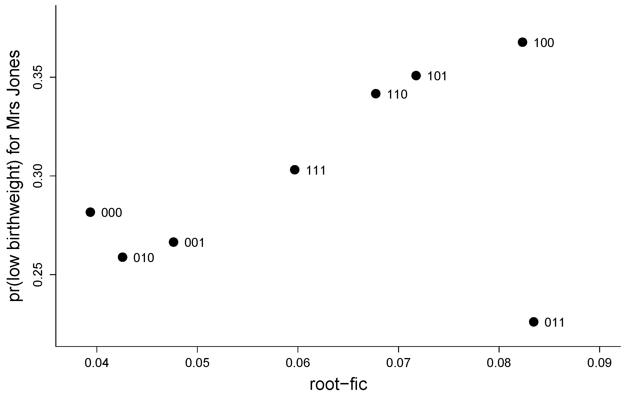
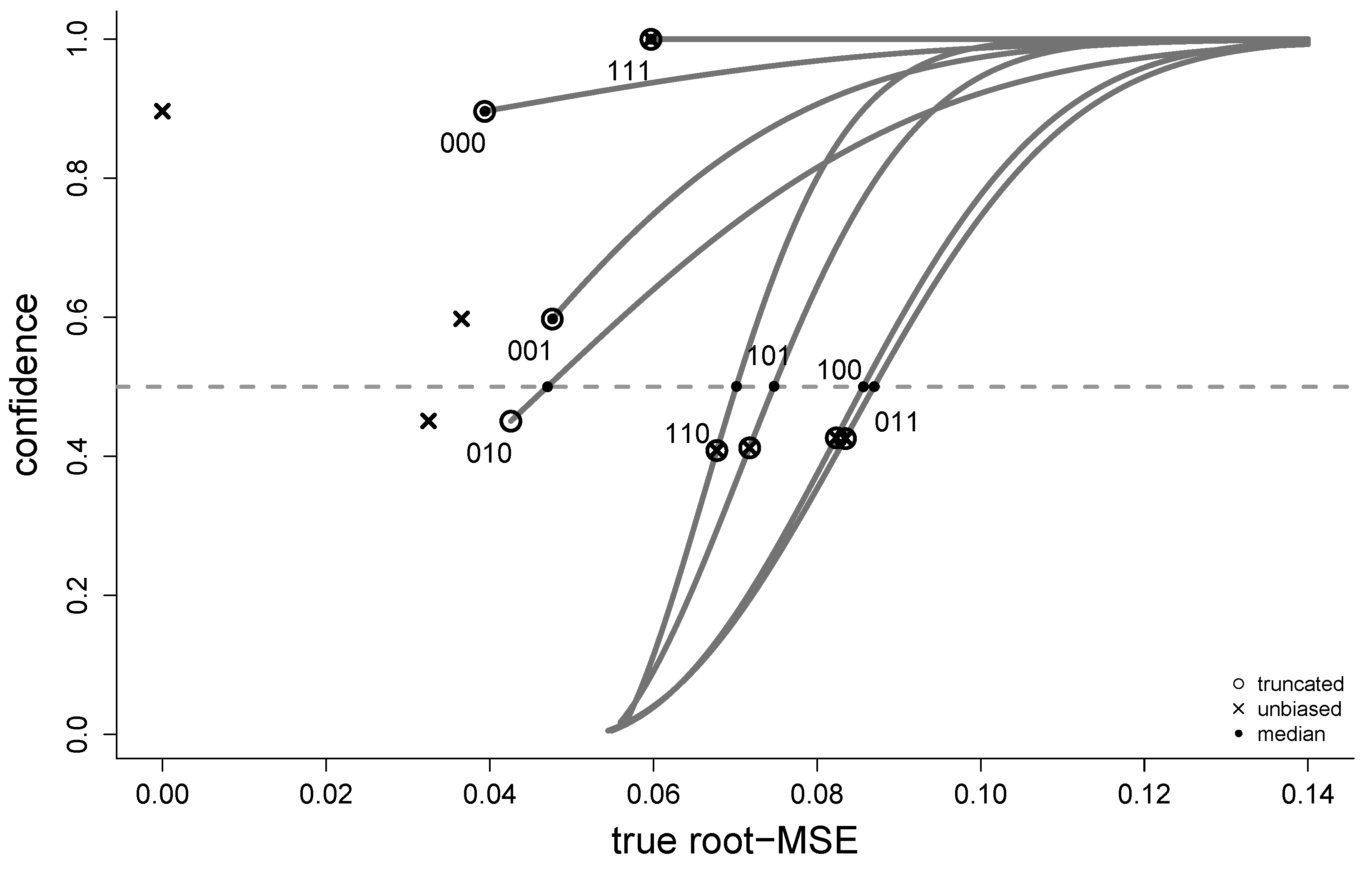
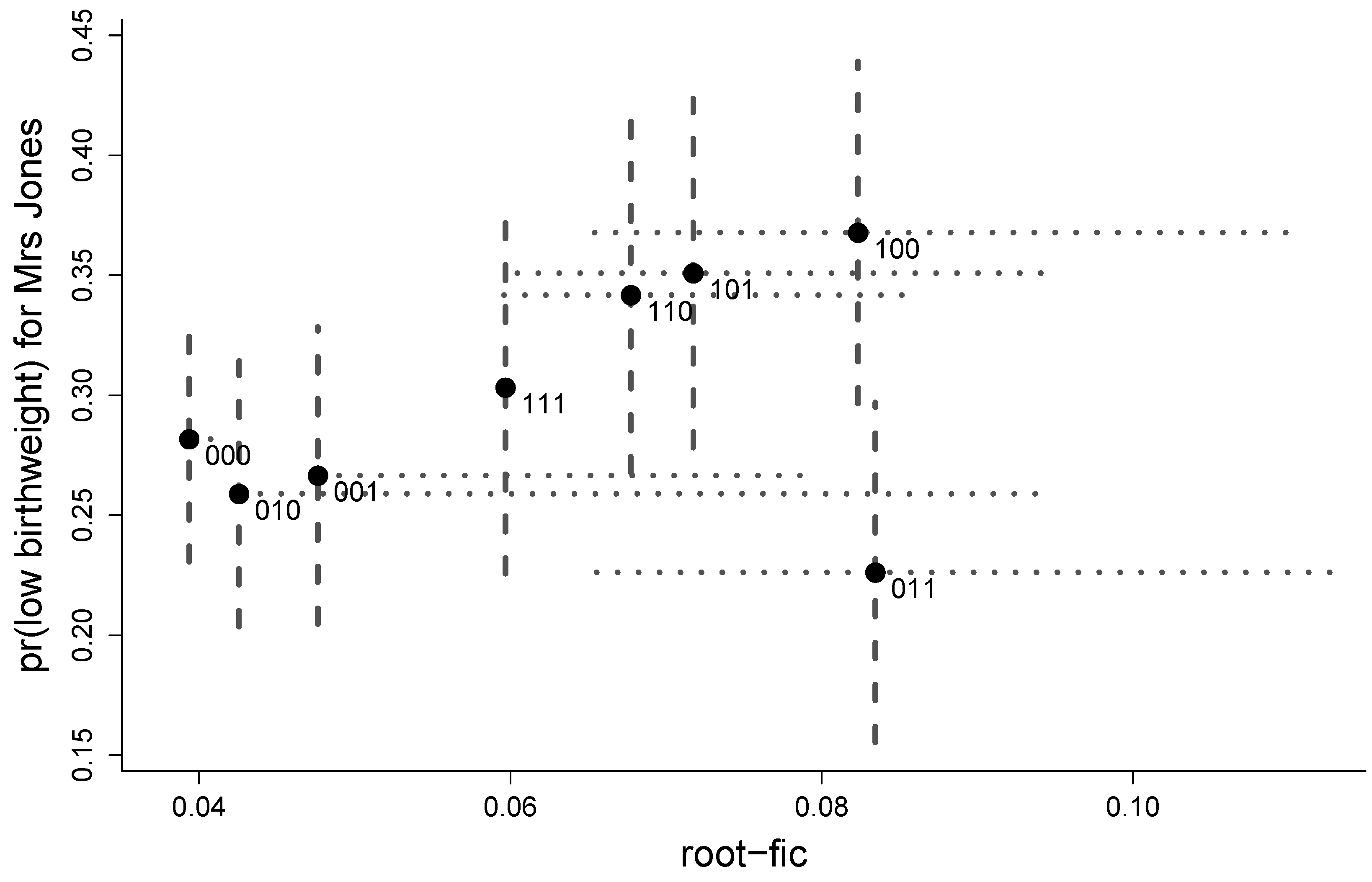
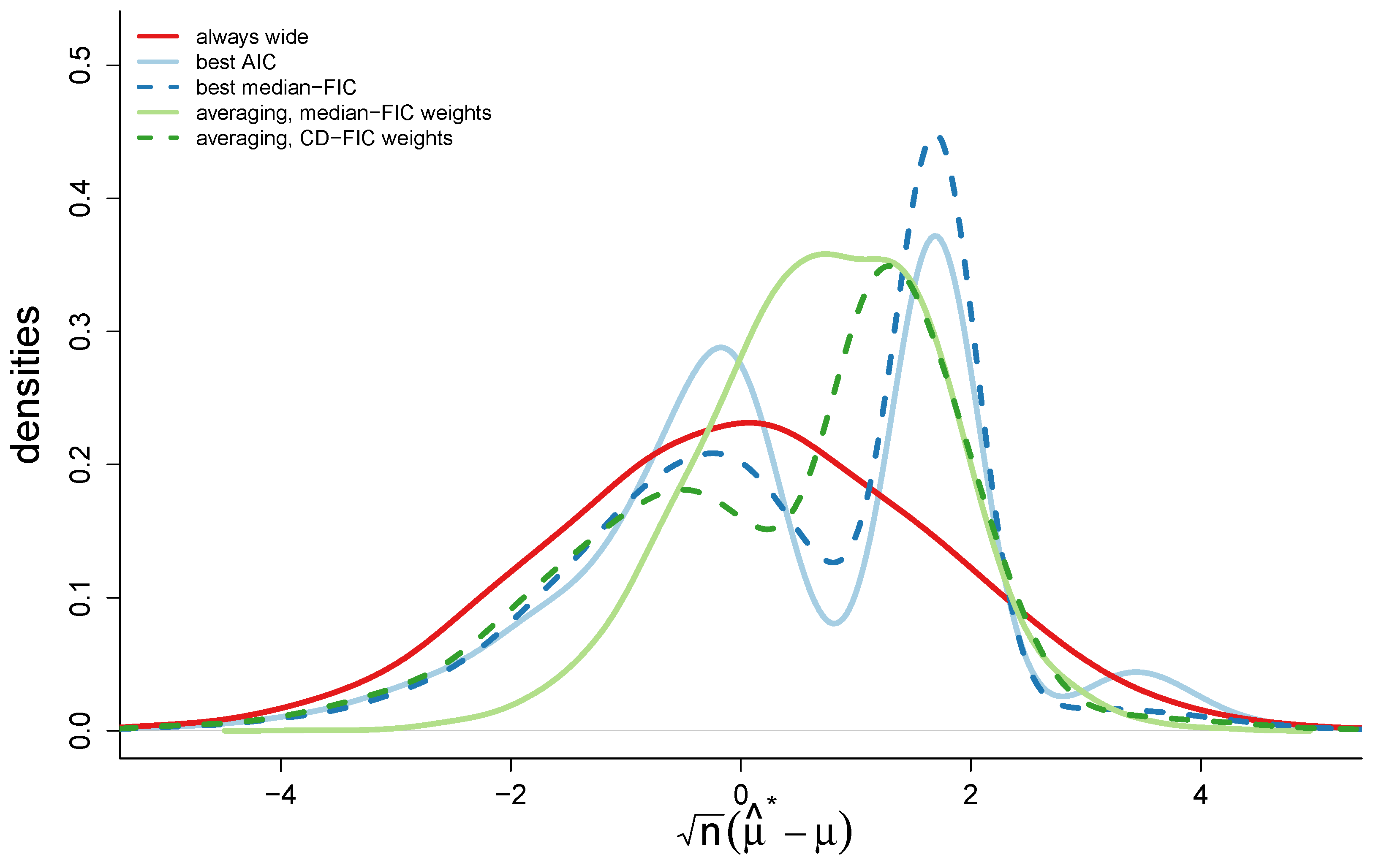
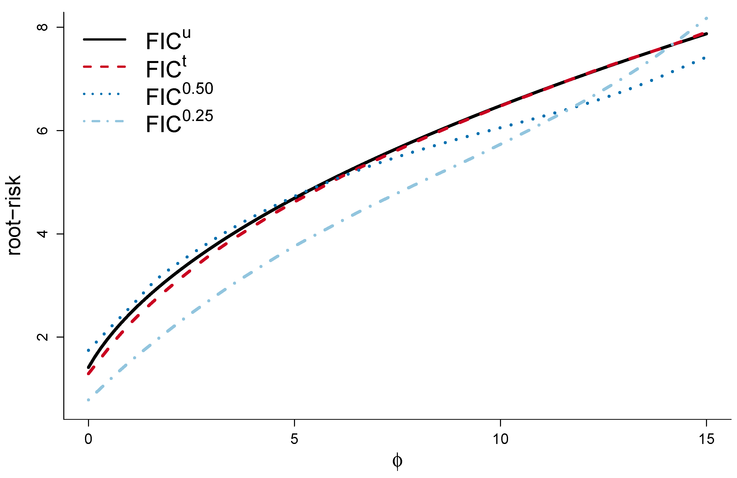
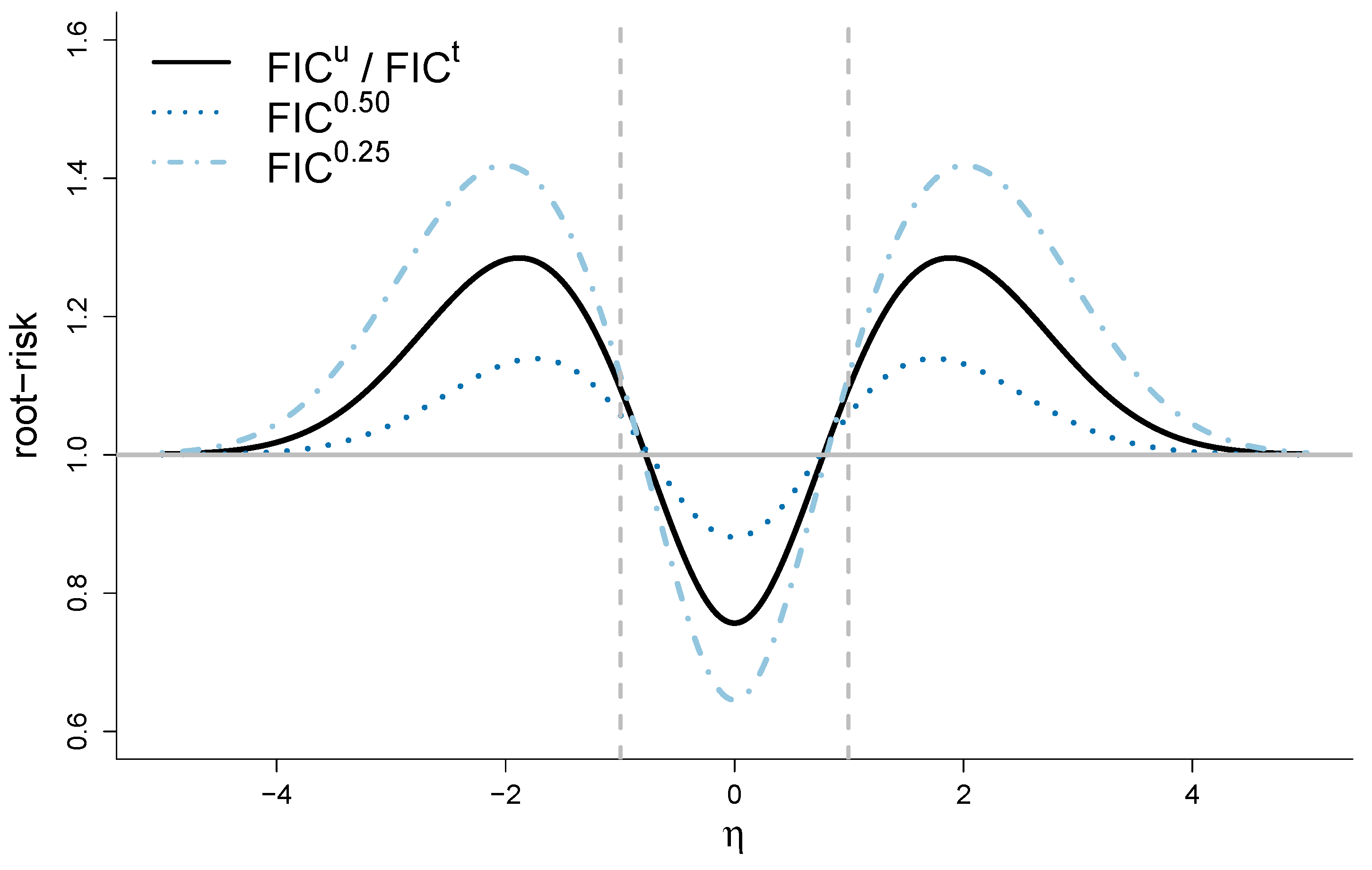
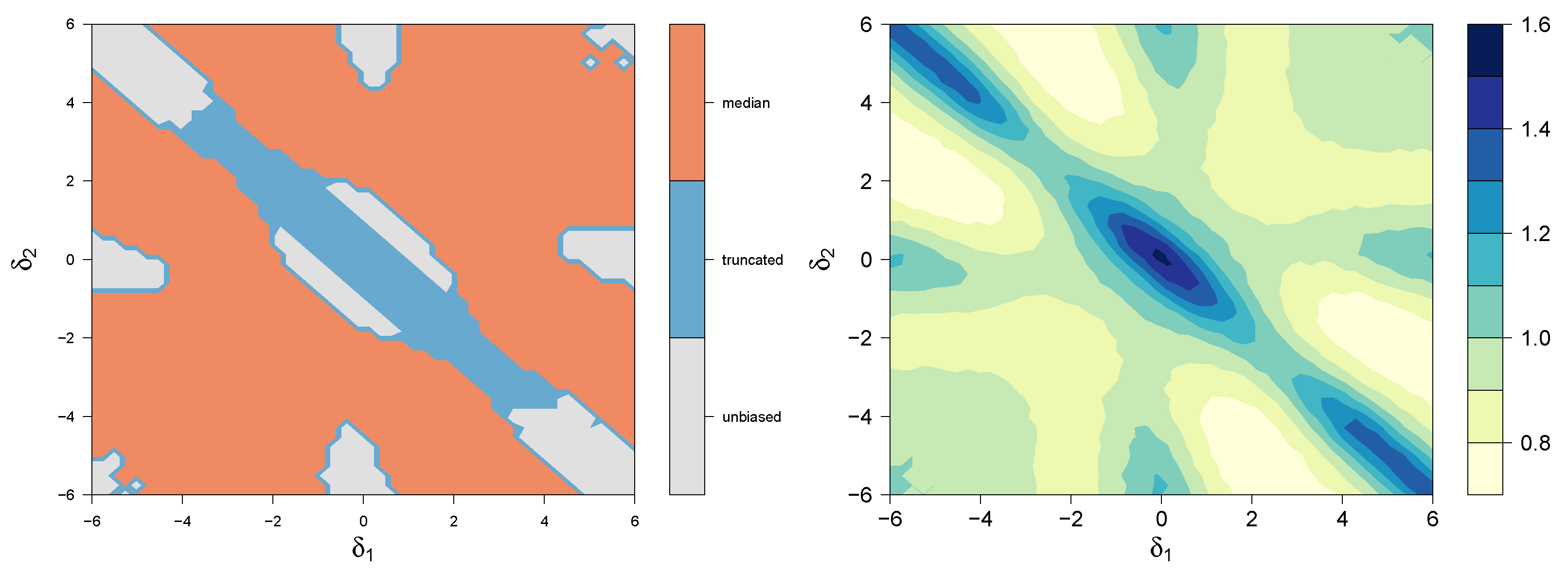
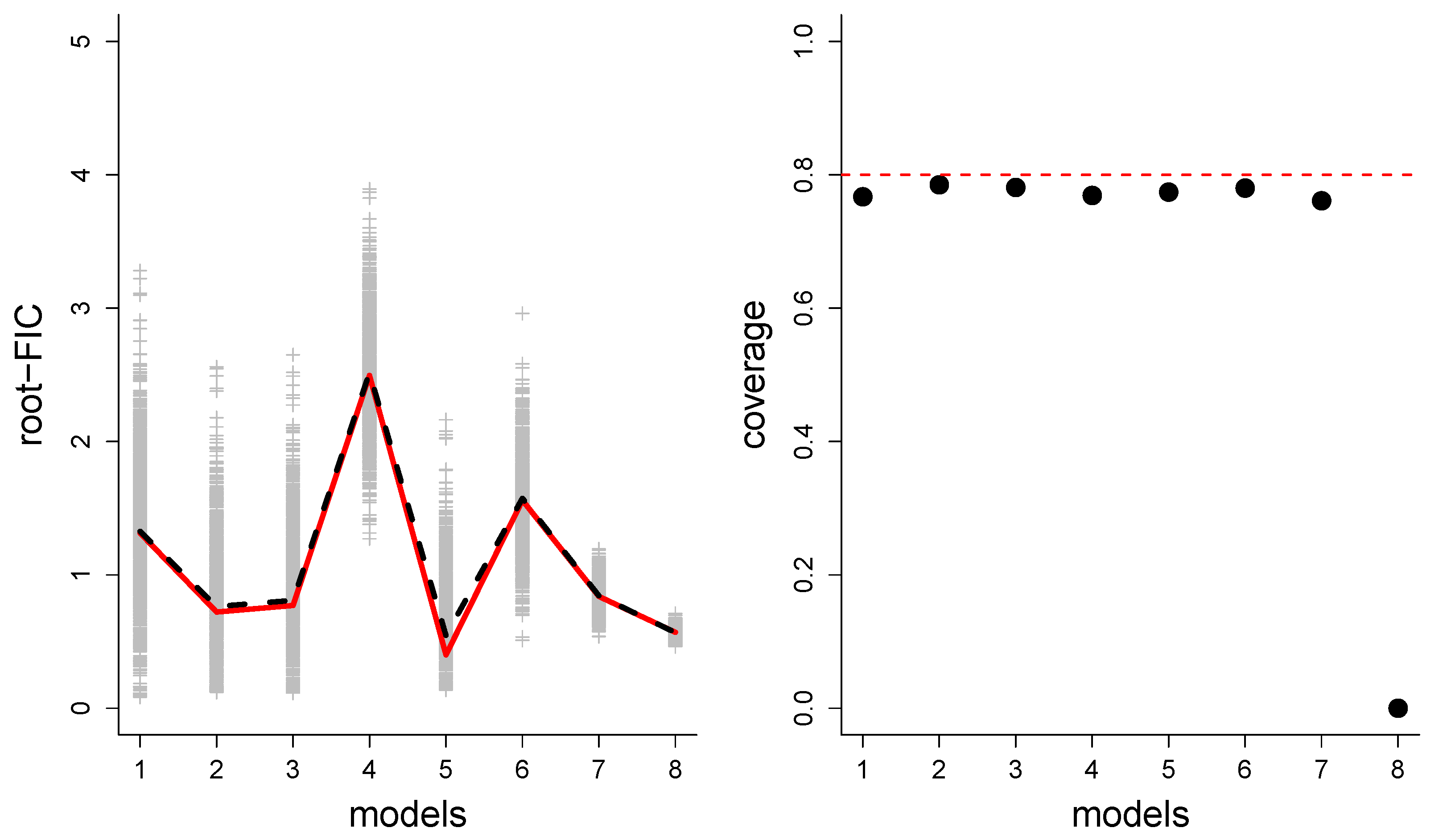
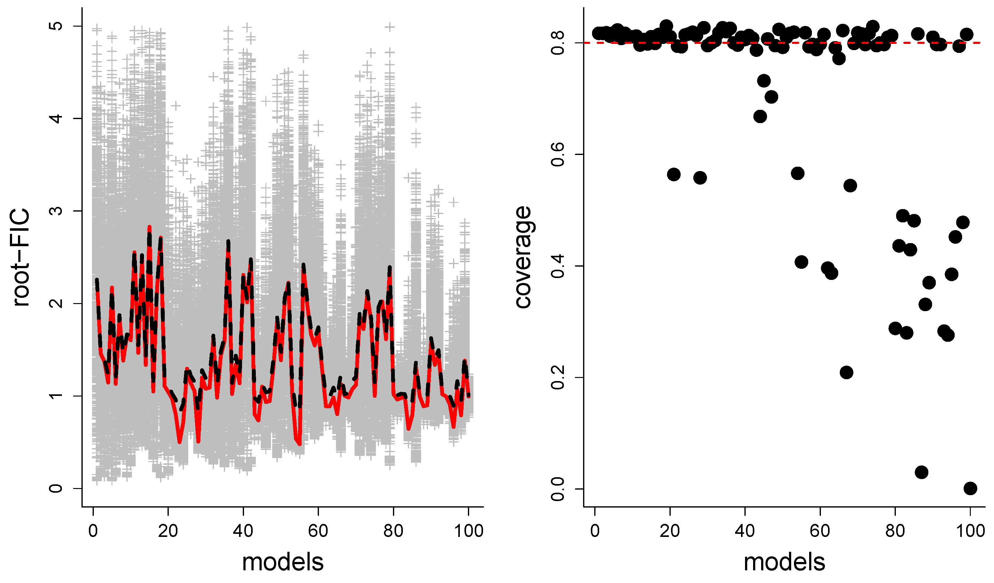
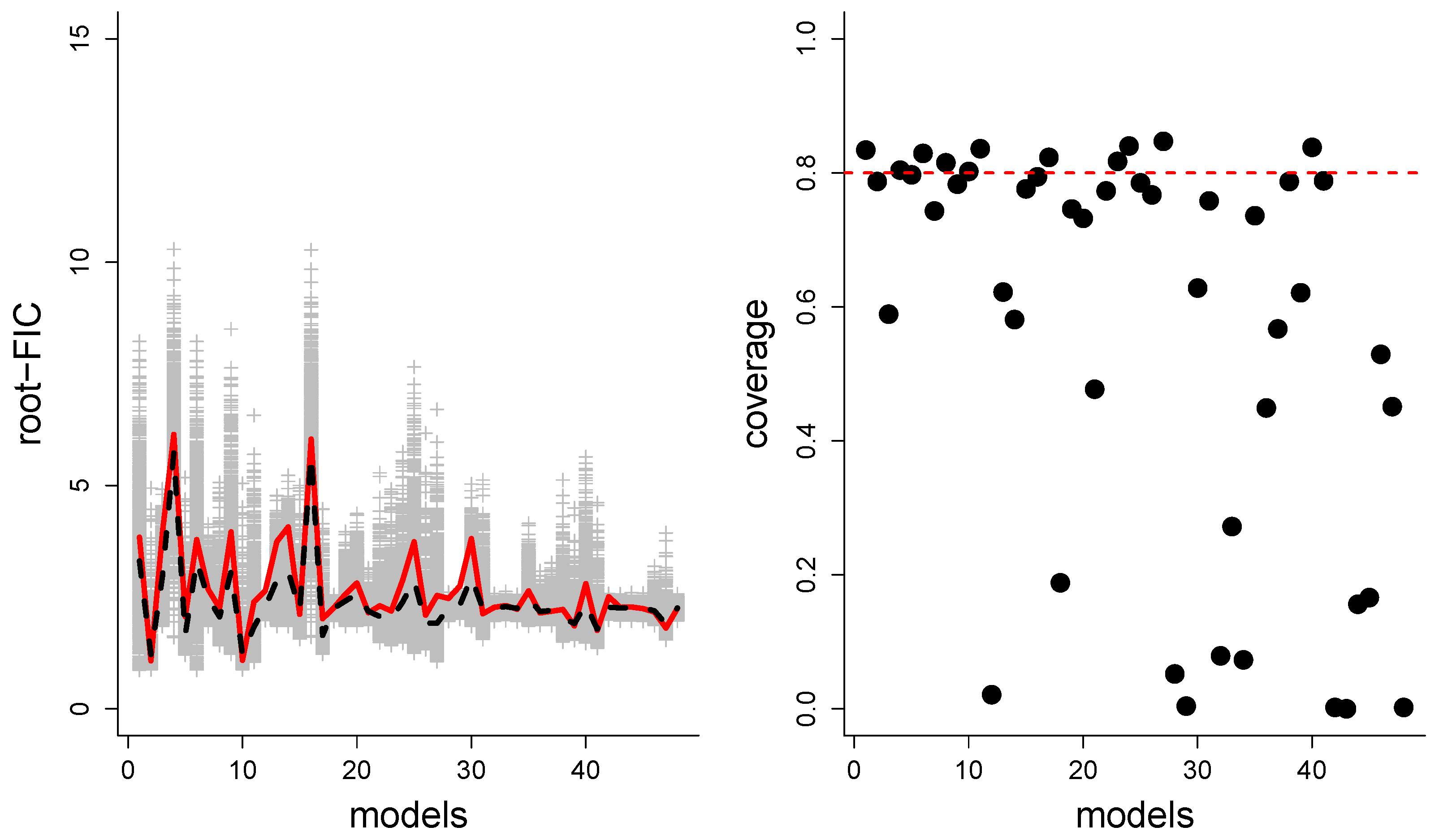
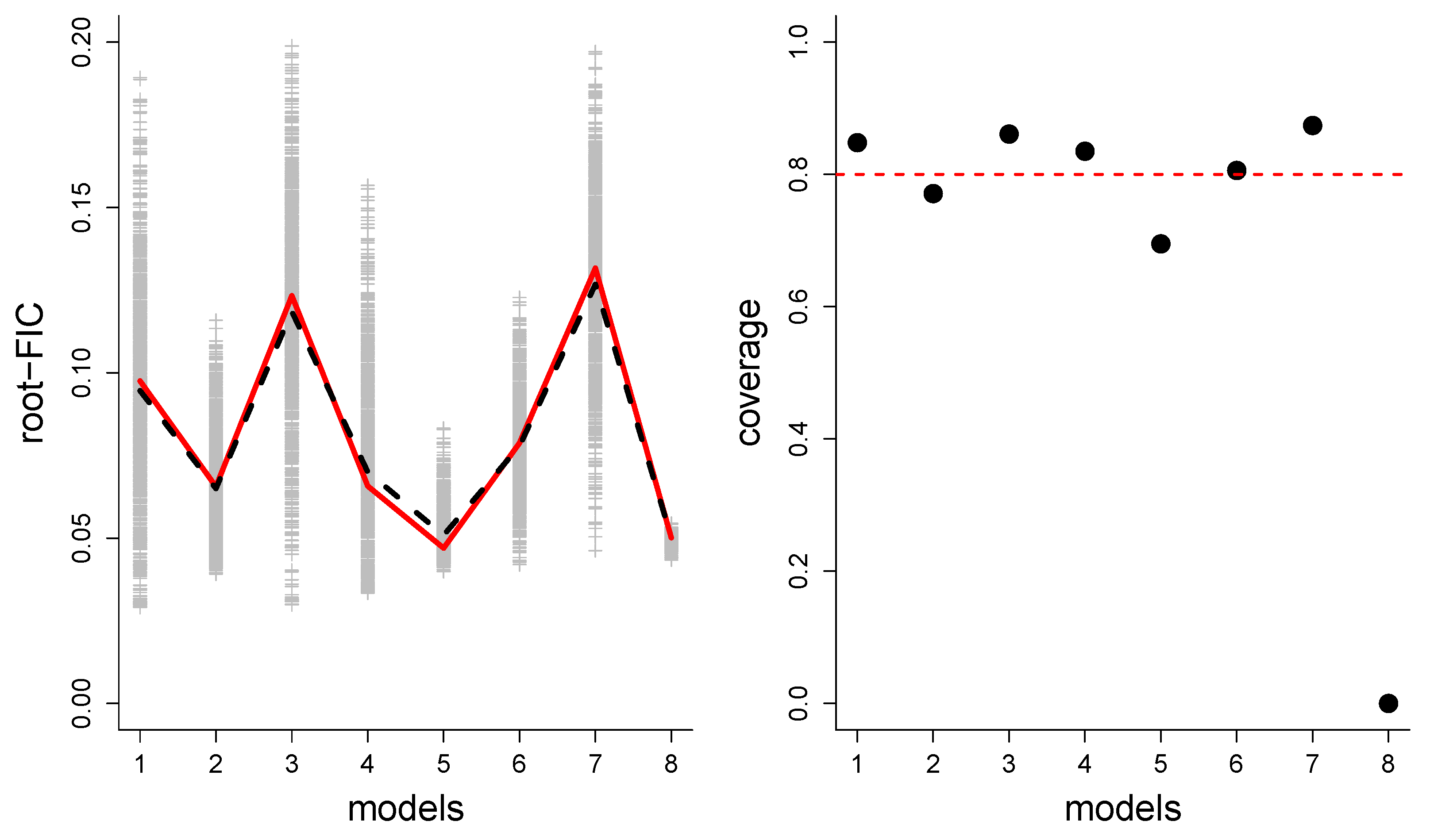
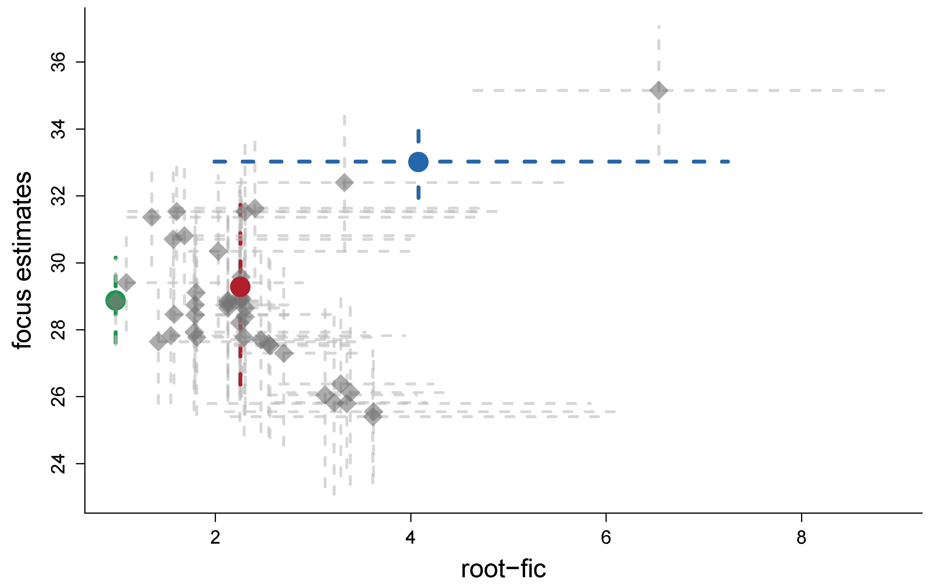
Table 1.
FIC table for Mrs. Jones: there are submodels, with absence-presence of indicated with 0 and 1 in column 2, followed by estimates , estimated standard deviation, estimated absolute bias, the root-FIC score, which is also the Pythagorean combination of the stdev and the bias, and the model rank. The numbers are computed with formulae of Section 2.
| in-or-out | Stdev | Bias | Root-FIC | Rank | ||
|---|---|---|---|---|---|---|
| 1 | 0 0 0 | 0.282 | 0.039 | 0.000 | 0.039 | 1 |
| 2 | 1 0 0 | 0.368 | 0.055 | 0.061 | 0.082 | 7 |
| 3 | 0 1 0 | 0.259 | 0.042 | 0.000 | 0.042 | 2 |
| 4 | 0 0 1 | 0.267 | 0.048 | 0.000 | 0.048 | 3 |
| 5 | 1 1 0 | 0.342 | 0.057 | 0.037 | 0.068 | 5 |
| 6 | 1 0 1 | 0.351 | 0.056 | 0.045 | 0.072 | 6 |
| 7 | 0 1 1 | 0.226 | 0.054 | 0.063 | 0.083 | 8 |
| 8 | 1 1 1 | 0.303 | 0.060 | 0.000 | 0.060 | 4 |
Table 2.
The percentage of rounds where each model has the lowest FIC score (i.e., the winning model). The first row is for setup (1), the second for setup (4).
Table 2.
The percentage of rounds where each model has the lowest FIC score (i.e., the winning model). The first row is for setup (1), the second for setup (4).
| (1) winning % | 5.5 | 6.1 | 18.1 | 0 | 32.0 | 0 | 0 | 38.3 |
| (4) winning % | 6.1 | 10.3 | 0.1 | 20.8 | 41.3 | 0.5 | 0 | 20.9 |
© 2020 by the authors. Licensee MDPI, Basel, Switzerland. This article is an open access article distributed under the terms and conditions of the Creative Commons Attribution (CC BY) license (http://creativecommons.org/licenses/by/4.0/).
Share and Cite
MDPI and ACS Style
Cunen, C.; Hjort, N.L. Confidence Distributions for FIC Scores. Econometrics 2020, 8, 27. https://doi.org/10.3390/econometrics8030027
AMA Style
Cunen C, Hjort NL. Confidence Distributions for FIC Scores. Econometrics. 2020; 8(3):27. https://doi.org/10.3390/econometrics8030027
Chicago/Turabian StyleCunen, Céline, and Nils Lid Hjort. 2020. "Confidence Distributions for FIC Scores" Econometrics 8, no. 3: 27. https://doi.org/10.3390/econometrics8030027
Note that from the first issue of 2016, this journal uses article numbers instead of page numbers. See further details here.