

Abstract
If high numerical apertures are used in coherence scanning interferometry, an extension of the interference signal's spectral distribution to lower frequencies can be observed. Depending on the slope of the measured surface interference signal contributions belonging to higher frequencies will vanish. In addition, the high spatial frequency information of a measured surface structure will contribute to the low frequency components of the spectrum of the measured interference signals. These effects can be explained by analyzing both the measuring object as well as the transfer characteristics of the interference microscope in the 3D spatial frequency domain. In this study we analyze the mentioned effects based on Kirchhoff's diffraction theory in the spatial frequency domain introducing the double foil model. The model explains why the choice of the wavelength, which is used for signal analysis, shows a substantial impact on the reconstructed topography. As a consequence, careful analysis of the 3D transfer function based on the Ewald sphere model enables a better understanding of the measuring process, the lateral resolution capabilities, and the improvement of the measurement results by choosing adequate signal processing parameters.
Export citation and abstract BibTeX RIS

Original content from this work may be used under the terms of the Creative Commons Attribution 4.0 license. Any further distribution of this work must maintain attribution to the author(s) and the title of the work, journal citation and DOI.
1. Introduction
Although coherence scanning interference microscopes are widely used in both scientific and industrial applications of topography measurement, the transfer characteristics of these instruments are mostly analyzed assuming that the resulting interference signals can be characterized by a constant central wavelength and an envelope representing the limited temporal and longitudinal spatial coherence of the light and the used illumination configuration [1]. This simplified approach works quite well for systems of low numerical aperture (NA) but needs at least a correction factor that transfers the wavelength of light into a so-called effective or equivalent wavelength  , if microscope objectives of higher NA are used in order to achieve better lateral resolution [2–5]. Recently, progress has been made in modeling and understanding the physical properties of coherence scanning interference microscopes. A first approach in this context that takes diffraction at the measured surface into account is based on Fourier optics [6–8]. The object is treated as a phase object, i.e. the optical field U0(x, y) on a surface s(x, y) immediately after reflection is given by:

where  represents the equivalent wave number
  related to the equivalent wavelength
  . For simplicity (1) assumes constant reflectivity of the surface and unit amplitude of the reflected field. Then the diffracted or scattered far-field is filtered in the spatial frequency domain due to the limited NA of the objective lens. This diffraction and filtering process occurs for all angles of incidence onto the object's surface as given by the incoherent Koehler illumination. In this case the transfer behavior of a coherence scanning interferometry (CSI) instrument can be obtained by pupil integration, i.e. incoherent superposition of plane wave contributions related to the pupil illumination [1, 8–11]. On the other hand, an analytical solution to this approach called approximate elementary Fourier optics (EFO) model uses the equivalent wavelength mentioned above in order to obtain an approximate transfer function for interference fringes in partially coherent light [7]. Approximating (1) in the limit of very small surface heights the complex scalar optical field U0(x, y) present on the object immediately after reflection is given by:

Following de Groot and Colonna de Lega [12] in this case the instrument transfer function (ITF) equals the incoherent optical transfer function MTF known from microscopic imaging given by the autocorrelation function of a 2D circular pupil [13].
Alternatively, to avoid the non-linearity due to the phase object according to (1) the object function o(x, y, z) can be interpreted as a Dirac function of the height coordinate z [14–16]:

Then (1) results via Fourier transform (FT) with respect to the z-axis:
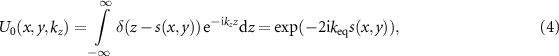
under the assumption  . The two-dimensional (2D) Fourier transform of (4) with respect to x and y yields the object spectrum
 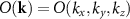 . Note that for a plane mirror-like surface in the xy-plane s(x, y) = 0 and thus
 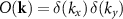 , i.e. there are no spatial frequency contributions in the
  -plane except for
  . As stated by several researchers [16–18] the multiplication of
  by the 3D transfer function
  of a CSI instrument leads to the interference term
  of the CSI signals in the spatial frequency domain (
 -space). The general concept of 3D transfer functions with respect to surface topography measuring instruments is discussed in a review article by Foreman et al [19]. According to Coupland, Su, Leach, de Groot et al [16, 17, 20–22] this concept corresponds to a linear filtering operation defined by a 3D convolution of the respective functions in the space domain, namely the Dirac function δ(z − s(x, y)) and the 3D point spread function (PSF) h(x, y, z), which represents the inverse 3D FT of
  .
.
The Dirac function in (4) describes the surface as an infinitesimally thin foil. This approach is known as foil model [16, 17]. It builds the basis of an analytical determination of the 3D transfer characteristics based on the Kirchhoff approximation (KA) for coherence scanning interferometers and other surface profiling instruments [16, 23, 24].
This model was recently used in CSI to correct 3D transfer and point spread characteristics [20, 25], to analyze defocus effects of the reference mirror [17] and to compensate for lens aberration [18].
In the following section we will modify the model with respect to CSI and discuss some aspects, which are especially relevant for the transfer characteristics of interference microscopes of high NA.
Nevertheless, it should be mentioned that the KA is strongly valid only if the minimum radii of curvature of the surface microstructure are much greater than the wavelength of light. If this criterion is violated the scattered light field in the spatial domain close to the surface needs to be calculated by a rigorous method in order to obtain quantitatively correct results [9, 26, 27]. Even though, the spatial frequency model discussed below still remains valid although the object spectrum will change. Furthermore, qualitative understanding can be achieved even if the surface under investigation does not strongly obey the assumptions of the KA.
2. Modelling based on Kirchhoff approximation and Ewald sphere analysis
Extending the Kirchhoff formulation of [15, 28, 29] with respect to our scattering geometry and for simplicity assuming a perfectly reflecting surface, a monochromatic plane wave of wavelength λ and wavenumber k0 = 2π/λ is incident under an angle  with respect to the global surface normal (z-direction) and an angle
  with respect to the xz-plane, as illustrated in figure 1. The scattered far-field
  in a plane at an angle
  with respect to the xz-plane and the scattering angle
  to the surface normal results from the integration:

where  including the wave vectors:
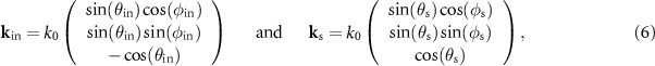
of the incident and the scattered wave, respectively. The area A of integration corresponds to the field of view of the interference microscope and  is a pupil function, which will be discussed later. The scattering geometry equals the configuration of Beckmann and Spizzichino [28] under the assumption
  , i.e. the xz-plane is the plane of incidence. For a surface, which is rough in the x-direction only, i.e. s(x, y) = s(x), the vector
  is given by:
Note that in this case the angle  depends on the scattering angle
  . In addition to the wave vector of a scattered wave, figure 1 shows the wave vector
  , which holds for specular reflection, i.e.
  . In this case the vector
  takes the simple form:
where  is the unit vector in z-direction. Due to the microscope arrangement,
  replaces the obliquity or inclination factor known from Kirchhoff diffraction theory [28]. The scattered field is normalized in a way that for a smooth surface and perpendicular incidence, i.e.
  , the amplitude in the specular direction becomes unity. Since this study aims at interference microscopes, an amplitude that changes with the angle of incidence can be considered by an appropriate pupil function [5].

Figure 1. Scattering geometry: (a) in the xz-plane, (b) in the xy-plane.
Download figure:
Standard image High-resolution imageAssuming constant illumination intensity over the pupil plane of the microscope objective lens using an aberration-free imaging system satisfying Abbe's sine condition for an arbitrary angle of incidence the reflected field in the specular direction results in [5]:

If  is assumed (5) represents the 2D FT of the phase object given by (1).
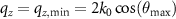
In order to analyze these relationships in more detail the Ewald sphere construction introduced for all wave vectors of scattered light considering all possible directions of incident waves is quite useful [30]. This concept has been extended by Quartel and Sheppard [23] to characterize the limitations of spatial frequency transfer of a conventional bright field microscope in  -space as it is shown in figure 2. Here, the maximum angle
  the incident and scattered waves include with the optical axis of the microscope objective lens is limited by its NA, i.e.
 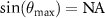 .
.

Figure 2. (a) Ewald sphere construction for a conventional microscope with the transfer function  assuming plane wave illumination incident under an angle
  and the transfer function
  taking all angles of incidence and all scattering angles that are covered by the objective's NA into account, (b) Ewald sphere construction showing the vertical line corresponding to specular reflection with point A belonging to perpendicular incidence and point B belonging to the marginal rays with
  , and points C and D corresponding to scattered light with
  and
and  .
.
Download figure:
Standard image High-resolution imageCoupland and colleagues use a similar concept to derive the 3D transfer function of CSI microscopes based on the foil model. They assume that the reference field equals the incident field multiplied by −1 [24, 16]. Recently, Su et al [17] and Thomas et al [26] applied this approach assuming that the negative wave vector  of the illumination wave equals the wave vector of the reference wave. Nevertheless, it should be possible to apply the foil model introduced so far to a perfectly aligned plane surface, i.e. s(x, y) = 0 in (4) and (5). Then for a sufficiently large field of view:
such that no contribution occurs for  .
.
However, Coupland et al [17, 24] attribute the function  they originally introduced as the transfer function of an axial holographic system with finite NA to the contribution of the reference wave. In this context a transfer function is defined as the system's response with respect to a single point scatterer represented by a 3D δ-function δ(x, y, z) at the input. Since a plane reference mirror differs from a single point scatterer, we have to modify the model in order to achieve full equivalence of the reference mirror's and the object's contribution to the interferometric image formation.
Due to the reflection at the reference mirror, according to figure 1 the wave vector  of the reference wave equals
  . This will be considered in the modified model introduced in the following. Nevertheless, determining the transfer characteristics of a CSI instrument assumes a spherical wave propagating from a (virtual) point source in the measurement arm for each reflected plane wave in the reference arm of the CSI instrument [24]. Due to the symmetry of the illumination pupil it does not matter whether
  , or
, or  . Under this assumption the transfer function obtained by Coupland et al [16] for a CSI instrument of a given
  can be written as a convolution of the transfer function
  and the set of incident plane waves
  as illustrated in figure 2(a). This results in the transfer function (TF)
  , which holds for a bright field reflective microscopic imaging system.
According to (6) the Cartesian components of the vector  are related to the angles of incidence and the scattering angles. Note, that due to the symmetry of a microscope objective lens,
  shows rotational symmetry with respect to the qz
-axis. Furthermore, the components qx
, qy
, qz
are not independent of each other. With respect to the TF we can combine the coordinates qx
and qy
by the new coordinate
shows rotational symmetry with respect to the qz
-axis. Furthermore, the components qx
, qy
, qz
are not independent of each other. With respect to the TF we can combine the coordinates qx
and qy
by the new coordinate  , representing the distance from the qz
-axis. This results in the following
, representing the distance from the qz
-axis. This results in the following  -vector:

As  according to (9) no longer depends on
  or
or  any cross section including the qz
-axis represents the complete TF. Note that the two components of
any cross section including the qz
-axis represents the complete TF. Note that the two components of  are still not independent of each other. In the backscatter direction, i.e.
  , the relationship
  holds.
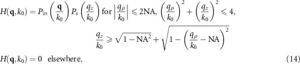
3. The 3D transfer function in interference microscopy
If we consider a real surface s(x, y) in the object arm of the measuring instrument, we have to assume  in order to assure that a perfectly adjusted reference mirror is mathematically treated in the same way as the surface of the measuring object. Note, that under the assumption of specular reflection all
  -vectors in figure 2(b) end on the qz
-axis between points A and B, where point A is related to normal incidence and B belongs to an angle of incidence of
-vectors in figure 2(b) end on the qz
-axis between points A and B, where point A is related to normal incidence and B belongs to an angle of incidence of  .
.
Considering two beam interference for a single angle of incidence the total intensity in the object space results in

where  and
and  are the object and the reference intensity, and the additional terms represent the interference contribution. U* denotes the complex conjugate of U. Note that for simplicity according to (1)
  and thus I0(x, y) = 1.
For a monochromatic wave incident under an angle  the third term can be written as:

where Δz is the difference of the depth scanner position along the z-axis with respect to the reference mirror's z-position.
Fourier transformation of  with respect to x and y leads to the correlation of the individual FTs
  and
and  :
:

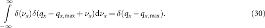
As interference occurs in the object or image plane (xy-plane), the correlation in the spatial frequency domain needs to be carried out in the  -plane. Fourier transformation of the fourth term in (10) results in:

Thus, the sum of the third and the fourth term leads to an even real part and an odd imaginary part in the spatial frequency domain. Hence, the total interference intensity contribution can be obtained from either the third or the fourth term in (10). Furthermore, since we assume incoherent Koehler illumination, interference occurs only on a spherical shell  related to a single vector
  according to figure 2(a). In addition, the reference field is characterized by specular reflection and for each incident wave represented by a Dirac function located on the qz
-axis, i.e. at
according to figure 2(a). In addition, the reference field is characterized by specular reflection and for each incident wave represented by a Dirac function located on the qz
-axis, i.e. at  . Consequently, the correlation leads to a Dirac function
  related to the object wave, multiplied by the corresponding complex amplitudes of the object and the reference field.
However, so far we have not considered the TF of the instrument. According to the projection-slice theorem [31] for incoherent imaging the integration of the transfer function  with respect to qz
corresponds to the well-known modulation transfer function [13] depending solely on qx
. Since the interference microscope is based on incoherent optical imaging [12], we first have to take the corresponding transfer function into account, introducing the 3D TF:
with respect to qz
corresponds to the well-known modulation transfer function [13] depending solely on qx
. Since the interference microscope is based on incoherent optical imaging [12], we first have to take the corresponding transfer function into account, introducing the 3D TF:
where  represents the pupil function of the incident wave,
  the pupil function of the scattered wave and the three conditions for
  determine the outer shape of the TF. Uniform illumination intensity in the pupil plane and constant
  according to figure 3(a) results in the angular intensity distribution
  , which needs to be considered as the illumination intensity decreases with an increasing angle
  [5, 32, 33]. This effect is referred to as photometric apodization [32] and the pupil function is given by:

Considering now a single point scatterer on the optical axis, i.e. at  the intensity scattered in an angular increment
  is independent of
  . Thus, the scattered intensity in the pupil plane increases as kx
increases, leading to the exit pupil function [32, 34]:
. Thus, the scattered intensity in the pupil plane increases as kx
increases, leading to the exit pupil function [32, 34]:

Therefore, the total pupil function in incoherent imaging  results in,

In order to calculate the value of the TF for a certain vector  related to a point Q of the TF we first have to obtain the corresponding angles of incidence and scattering. A sketch of the configuration is shown in figure 3(b). The points of intersection of circles of radius k0 centered around the origin and point Q are the end points of the two vectors
  and
and  and the starting points of the vectors
  and
and  . These vectors demonstrate that each point Q of the TF can be reached by two different ray paths in the
  -plane. Due to the symmetry of the configuration the values of the angles θ1 and θ2 are the same and can be obtained by:

where  Further, the angle α is given by:

This leads to the angles of incidence:
Due to the symmetry the corresponding scattering angles follow:
Thus, the TF for incoherent imaging finally results in:
where the factor 1/2 normalizes the TF so that  . This function is displayed in figures 4(a) and 5(a) for
  and
and  , respectively. Note that the above calculation takes ray paths only in the
  -plane into account. Therefore, the TF according to (22) is an approximation demonstrating the effect of photometric apodization. For an exact computation figure 3(b) needs to be extended to three dimensions such that the two intersecting circles become spheres and the end and starting points of the vectors contributing to the intensity at point Q are on a circle. If these out of plane contributions are considered the effect of photometric apodization will decrease since the corresponding ratios
  will be closer to one.

Figure 3. (a) Geometry explaining the effect of photometric apodization in high NA imaging. (b) Geometrical arrangement for the reconstruction of the angles of incidence  and the scattering angles
  corresponding to a given point of the transfer function in the spatial frequency domain.
Download figure:
Standard image High-resolution image
Figure 4. Cross sectional views of the transfer functions  for
for  : (a)
: (a)  for incoherent imaging, (b) deviation of
  from a unity TF (the color of the background area outside the Ewald sphere corresponds to zero for better perceptibility of the deviations), (c)
  for the interference component, (d) difference
  .
.
Download figure:
Standard image High-resolution image
Figure 5. Cross sectional views of the transfer functions  for
for  : (a)
: (a)  for incoherent imaging, (b) deviation of
  from a unity TF (the color of the background area outside the Ewald sphere corresponds to zero for better perceptibility of the deviations), (c)
  for the interference component, (d) difference
  .
.
Download figure:
Standard image High-resolution imageFigures 4(b) and 5(b) show the deviation of  from a unity TF, which holds for small
  -values, where
  . The more the NA increases the more the imaging TF deviates from the unity TF. However, in order to obtain the TF for the interference component, we have to consider correlations of the square root of the incoherent imaging TF introduced so far and the corresponding contributions of the reference mirror on a spherical shell. Due to the specular reflection, the
  -space intensity of the reference mirror is represented by δ-functions
  with amplitudes solely depending on the qz
-coordinate so that the correlations result in multiplications. According to the photometric apodization [32, 34] (see figure 3(a)) this intensity is proportional to
with amplitudes solely depending on the qz
-coordinate so that the correlations result in multiplications. According to the photometric apodization [32, 34] (see figure 3(a)) this intensity is proportional to  (see equation (15)). Therefore, in agreement with [5, 14, 33] the corresponding reference intensity is proportional to the qz
-value. If this is taken into account, the following TF results for the interference contribution:
(see equation (15)). Therefore, in agreement with [5, 14, 33] the corresponding reference intensity is proportional to the qz
-value. If this is taken into account, the following TF results for the interference contribution:
Transfer functions for the interference component are shown in figure 4(c) for  and figure 5(c) for
  . Since the intensity contribution of the reference mirror is proportional to qz
, the whole TF increases along the qz
axis. This can be seen in figures 4(d) and 5(d), which represent the difference of the TFs for incoherent imaging and those derived for the interference component.
. Since the intensity contribution of the reference mirror is proportional to qz
, the whole TF increases along the qz
axis. This can be seen in figures 4(d) and 5(d), which represent the difference of the TFs for incoherent imaging and those derived for the interference component.
The CSI model introduced here is summarized in figure 6. Since both the surface under investigation as well as the surface of the reference mirror are mathematically described by thin foils, the model is called double foil model.

Figure 6. General procedure of 3D interference image stack generation based on the double foil model.
Download figure:
Standard image High-resolution imageAll contributions of the reference wave are located on the qz
-axis and, therefore, the correlation of the reference mirror's and object's contributions in the  -plane does not change the final result, except for the pupil function of the reference wave, which needs to be considered. The interference intensity image stack I(x, y, z) follows as the real part from the inverse 3D FT of the following equation:

where ![$[ \ldots ]_{q_x,q_y}$](https://content.cld.iop.org/journals/2515-7647/3/1/014006/revision3/jpphotonabda15ieqn124.gif) denotes that the correlation is carried out with respect to qx
and qy
and the second equal sign holds only if unity amplitude of
denotes that the correlation is carried out with respect to qx
and qy
and the second equal sign holds only if unity amplitude of  is assumed considering the qz
-dependence of the reference contribution as part of
is assumed considering the qz
-dependence of the reference contribution as part of  .
.
Since  shows rotational symmetry its inverse FT with respect to qx
and qy
is real-valued. The inverse 3D FT of the object spectrum
shows rotational symmetry its inverse FT with respect to qx
and qy
is real-valued. The inverse 3D FT of the object spectrum  equals the real-valued function o(x, y, z). Therefore, inverse FT of (24) leads to:

i.e. the 3D-interference pattern in the spatial domain equals a convolution of the surface foil and the real part of the function  resulting from the inverse 3D FT of
  . Note that
  represents the PSF only as long as the surface under investigation consists of single point scatterers. This is due to the fact that the coordinates
  and qz
of the TF are not independent as will be further discussed in the next section.
and qz
of the TF are not independent as will be further discussed in the next section.
The procedure of 3D interference pattern formation summarized in figure 6 can be easily extended in order to consider a tilted reference mirror or a reference surface  , which differs from a plane mirror [35]. In addition, the central obscuration introduced in the reference and the object wave fields by the reference mirror in a Mirau objective can be considered by its pupil function [5]. Furthermore, the limited temporal coherence of a light source can be taken into account by integration of
  for different wavenumbers k0 and appropriate weighting [16, 24]. Since the coherence envelope is multiplied to an interference signal in the spatial domain, this can be considered by a convolution with the corresponding spectral density function in the spatial frequency domain.
4. Analysis of the 3D transfer function by examples
4.1. Mirror-like object surfaces
If we assume a perfectly adjusted plane mirror instead of the point scatterer even in the object arm of the interferometer, the physical configuration of the measurement and the reference arm is exactly the same. Thus, if in analogy with Su, Thomas et al [17, 26]  is assumed we would have to set
  too, since
  is the wave vector describing the wave propagation of the scattered/reflected wave in the measurement arm. Following the conventional foil model the convolution of the object and the reference field then results in vectors that end on the outer spherical shell with radius 2k0 according to figure 2. Consequently, for all angles of incidence different from zero non-zero spatial frequency components kx
or ky
occur, which lead to interference fringes that cannot be observed in reality under these assumptions.
is the wave vector describing the wave propagation of the scattered/reflected wave in the measurement arm. Following the conventional foil model the convolution of the object and the reference field then results in vectors that end on the outer spherical shell with radius 2k0 according to figure 2. Consequently, for all angles of incidence different from zero non-zero spatial frequency components kx
or ky
occur, which lead to interference fringes that cannot be observed in reality under these assumptions.
If we apply the double foil model introduced in the section above, where both the object and the reference wave are treated in the same way using the sum of two wave vectors, i.e.  , a correlation of two Delta functions on the qz
-axis results and the whole interference intensity distribution is located between points A and B on the qz
-axis in figure 2(b). This intensity represents the power spectral density of the electric field. Thus, following the Wiener-Khintchin theorem, the real part of the inverse FT with respect to the qz
-coordinate leads to the autocorrelation function of
, a correlation of two Delta functions on the qz
-axis results and the whole interference intensity distribution is located between points A and B on the qz
-axis in figure 2(b). This intensity represents the power spectral density of the electric field. Thus, following the Wiener-Khintchin theorem, the real part of the inverse FT with respect to the qz
-coordinate leads to the autocorrelation function of  along the z-axis, whereas the amplitude in the xy-plane is constant considering the 3D-representation.
The object and the reference field can be obtained from (5) assuming s(x, y) = 0:

Considering (14) and the fact that,

the pupil function  used in (26) is in agreement with [5, 33] given by:

Figure 7 shows the spectrum and the corresponding interference signal obtained via FT with respect to the qz -coordinate, which holds for all x, y ∈ A, assuming s(x, y) = 0. In addition, in figure 7(b) a signal with a sinc-shaped envelope is plotted, which occurs for constant intensity of the incident light over the angle of incidence known as the Herschel condition [1, 5].

Figure 7. Ramp-shaped power spectral density along the qz -axis (a) and the corresponding autocorrelation function representing the interference signal along the position of the depth scanner compared to a signal with sinc-shaped envelope corresponding to a rectangular spectrum (b).
Download figure:
Standard image High-resolution imageNote that the convolution of the signal for the ramped-shaped spectrum with a δ-function located at z = 0 representing the surface according to the foil model leads to the image stack I(x, y, z) for a perfectly adjusted plane mirror. Thus, the 3D image stack is not affected by any value of  with
with  different from zero. Consequently, this image stack I(x, y, z) will not follow from a convolution operation with the general PSF
  defined as the inverse 3D FT of
  .
.  is affected by all values of
  , which are different from zero including those, where
  . In addition, the section along the qz
-axis, where
. In addition, the section along the qz
-axis, where  differs from the section, where
  .
.
If we further assume  , according to (8) all energy will be concentrated at
  , i.e. the distribution in the
  -plane corresponds to a δ-peak resulting in a cosinusoidal autocorrelation function:

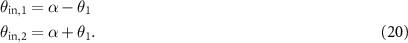
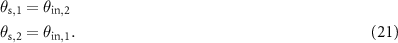
The situation changes if the mirror-like surface representing the measurement object is tilted. Then the δ-peak corresponding to the reflected wave in the object arm is no longer located on the qz
-axis, whereas the reflected wave in the reference arm still is. We assume that the normal to the surface is tilted in the xz-plane with respect to the z-axis by an angle  . Then the reflection with respect to the y-coordinate remains unchanged and the reflected wave will propagate under an angle
 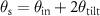 . Thus, the
  -space coordinates corresponding to the reflected wave in the object arm are given by
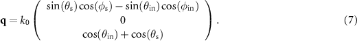
 ![$q_x(\theta_{\mathrm{in}},\theta_{\mathrm{tilt}}) = k_0 [\sin(\theta_{\mathrm{in}})-\sin(\theta_{\mathrm{in}}+ 2\theta_{\mathrm{tilt}})]$](https://content.cld.iop.org/journals/2515-7647/3/1/014006/revision3/jpphotonabda15ieqn156.gif) ,
, ![$q_z (\theta_{\mathrm{in}},\theta_{\mathrm{tilt}}) = k_0 [\cos(\theta_{\mathrm{in}})+\cos(\theta_{\mathrm{in}}+ 2\theta_{\mathrm{tilt}})]$](https://content.cld.iop.org/journals/2515-7647/3/1/014006/revision3/jpphotonabda15ieqn157.gif) .
.
This results in a δ-function located at  ,
,  representing the reflected object wave, which is correlated with respect to the qx
-coordinate with another δ-function located at qx
= 0,
representing the reflected object wave, which is correlated with respect to the qx
-coordinate with another δ-function located at qx
= 0, 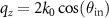 representing the reference wave. In the extreme situation
  and
and  shown in figure 8(a) it follows that
  and
and  .
.

Figure 8. (a) Interference intensity distribution for a plane mirror with 64∘ tilt assuming  , (b) for a weak phase grating with first order diffraction at −64∘ (backscattering direction).
Download figure:
Standard image High-resolution imageThe correlation results in:
Since 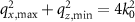 , the oblique wave is represented by a δ-function depending on qz
, too. Consequently, the combined δ-function is located at
, the oblique wave is represented by a δ-function depending on qz
, too. Consequently, the combined δ-function is located at 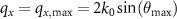 ,
,  and its inverse FT results in:

Thus, the interference signal takes the form:

where z = s(x)−Δz and  represents the value of the TF at point D according to figure 2(b). This leads to the interference pattern displayed in figure 8(a). Note that the period along the z-axis is more than two times λ/2, i.e. the effective wavelength is more than twice the physical wavelength λ. The effect of surface tilt on the shift of the corresponding signal spectrum and the resulting fringe spacing has been considered previously by introducing an appropriate
  factor [5].
From (32) we further obtain the following relationship for the zero phase:

Equation (32) can be written as a 3D convolution introduced in (25), where  is the surface foil and
  is z-component of the inverse FT of the relevant
  cross section of the TF, which will be introduced in section 4.3 as partial 3D PSF. Note that this function differs from the PSF derived by 3D FT of
  as it comprises only the cos-term for the single spatial frequency
  . Furthermore, the surface under investigation is specularly reflecting and thus the value of
  , which defines the amplitude of the cos-term, needs to be replaced by
  , which holds for specular reflection. This example demonstrates that the general approach of obtaining the response of an ideal CSI instrument by a linear filtering operation defined by a convolution with a universal PSF does not work here since the
  -space variables are not independent of each other.
If the surface tilt angle is smaller than  (32) and (33) lead to:

This behaviour can be observed in the experimental result displayed in figure 12(b). The values, which differ from zero, show the proportionality of qz and qx .
4.2. Gratings and lateral resolution
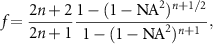
Grating structures are often used to determine the lateral resolution capabilities of CSI instruments. According to Abbe's theory of microscopic image formation a grating structure will be resolved as long as at least the zero order and the plus or minus first order diffracted light will pass the aperture of the objective lens and thus contribute to the image. This leads to the well-known Abbe limit  , which establishes the minimum grating period
  resolved by an objective of given
  using the illumination wavelength λ. It should be noted that in the context of this paper the grating is a phase grating of the form
  , which generally provides diffraction orders higher than ±1 even if s(x, y) is a sinusoidal function [12]. According to the above sections the maximum spatial frequency of a one-dimensional grating structured along the x-axis, which may be resolved by a CSI instrument, is
  . In this case we will find a δ-function at point D in figure 2(b) representing the backscattering direction for the minimum angle of incidence
  limited by the
  . In contrast to the situation for a tilted surface, however, the zero order diffracted object wave will cause another δ-function located at qx
= 0 (point B in figure 2(b)) and backscattering for the maximum angle of incidence leads to a δ-function located at
. In contrast to the situation for a tilted surface, however, the zero order diffracted object wave will cause another δ-function located at qx
= 0 (point B in figure 2(b)) and backscattering for the maximum angle of incidence leads to a δ-function located at  corresponding to point C in figure 2(b). This consideration agrees to Abbe's theory since,

A simulation of this situation leads to the interferogram depicted in figure 8(b), where the grating structure can be recognized and the fringe spacing in z-direction is the same as in figure 8(a).
Again, it is important to realize that the coordinates qx
and qz
are not independent. From  it follows that
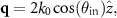
  . As mentioned in section 1, one can write the average spatial frequency
  in terms of an equivalent wavelength, i.e.
  . In the same manner we can express an arbitrary value of qz
by a so-called evaluation wavelength
. In the same manner we can express an arbitrary value of qz
by a so-called evaluation wavelength  , leading to

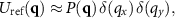
In CSI signal processing an interference signal  recorded by a single camera pixel at
  is typically analyzed assuming a certain wavelength, i.e. phase analysis is performed at the center wavelength
  of the signal (e.g. [36, 37]). However, also wavelengths
  different from
  can be chosen for phase analysis.
Coming back to the current situation we can define the maximum evaluation wavelength by:

For  the maximum evaluation wavelength is
 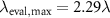 . This means that analyzing the smallest surface period requires an evaluation wavelength of 2.29 times the illumination wavelength. As a consequence, in order to find the grating structure in the interference signals according to figure 8(b) requires phase analysis at
  . Figure 9(a) shows the general dependence of the of the evaluation wavelength on qz
for λ = 450 nm and
. Figure 9(a) shows the general dependence of the of the evaluation wavelength on qz
for λ = 450 nm and  . In addition, we can obtain the lateral resolution for a given evaluation wavelength using (35) and (37):
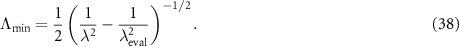
Equation (38) reveals that the smallest lateral resolution requires the longest evaluation wavelength. This is plotted in figure 9(b), and has been discussed already in earlier publications [38, 39]. However, the lateral resolution of a 2D microscope is not necessarily the same as the lateral resolution in 3D microscopy. If the surface under investigation is a phase grating with a spatial frequency that is damped by the TF  an underestimation of the surface amplitudes is to be expected. Furthermore, the shape of the grating structure reconstructed from the measurement result will differ from the real structure due to the low-pass filtering effect of the TF. Of course, the underestimation can be reduced by compensating for the influence of the TF [20], but diffraction orders not collected by the NA of the objective lens will be lost. Additionally, the TF related to a deterministic grating will differ from the TF of a point scatterer and depends on further apodization effects if the pupil illumination is not constant.

Figure 9. (a) Evaluation wavelength as a function of qz
and (b) lateral resolution depending on the evaluation wavelength assuming  and λ = 450 nm.
Download figure:
Standard image High-resolution image4.3. PSFs and lateral resolution
The 3D PSF results from 3D FT of the TF shown in figures 4(c) and 5(c). For a physical understanding we analyze cross sections of the TF, which are in parallel to the  -plane. Each of these cross sections is characterized by a constant qz
-value, which after Fourier transformation with respect to qz
represents the angular frequency of a cosine function along the z-axis. Since these cross sections are of rotational symmetry with respect to the qz
-axis the overall extension of such a disc along the
-plane. Each of these cross sections is characterized by a constant qz
-value, which after Fourier transformation with respect to qz
represents the angular frequency of a cosine function along the z-axis. Since these cross sections are of rotational symmetry with respect to the qz
-axis the overall extension of such a disc along the  -coordinate determines the lateral resolution, which is thus coupled to the corresponding qz
-value. All points located in
-coordinate determines the lateral resolution, which is thus coupled to the corresponding qz
-value. All points located in  -space on an outer circle of given radius correspond to backscattered wave contributions according to figure 2(b). Therefore, these points are characterized by a constant angle of incidence
  and an equal scattering angle, i.e.
  ,
,  and
and 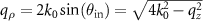 .
.
Sheppard and Larkin [5] introduce the  -factor:
which describes the increasing fringe spacing depending on the NA of the optical system and the apodization exponent n. For an aplanatic imaging system in accordance with (8) n = 1/2. If we now chose the angle of incidence such that  , we can obtain qz
(f) and
, we can obtain qz
(f) and  , the equivalent wavelength
  and the Airy disc function corresponding to an aperture of radius
  . This represents the PSF in the xy-plane:

which is denoted PSF 1 in figure 10(a). This PSF is normalized to a maximum value of 1, assuming  and a
and a  -factor f = 1.325, which holds for n = 1/2 and
  [5]. The corresponding plane of constant qz
is indicated in figure 2(b) as equivalent wavelength plane. Note that the cross section of
[5]. The corresponding plane of constant qz
is indicated in figure 2(b) as equivalent wavelength plane. Note that the cross section of  is nearly constant for
 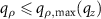 . Hence the corresponding PSF 1 according to figure 10(a) equals the inverse FT of a circular disc function and (39) may reach negative values.

Figure 10. (a) 2D PSFs resulting from 2D FT of the TF at different cross sections of constant qz
, (b) cross section of the 3D PSF corresponding to (40) with an equivalent evaluation wavelength of  , where black and white areas are attributed to −1 and +1, respectively, (c) cross section of the 3D PSF corresponding to (43) using the maximum evaluation wavelength of
  .
.
Download figure:
Standard image High-resolution imageThe 3D PSF plotted in figure 10(b) then takes the form:

The radius of the effective aperture  leads to the effective numerical aperture
  , which defines the lateral resolution instead of the full
  of 0.9. The argument of the cosine function is related to the equivalent wavelength
  by:
by:

used in practice to analyze the phase of the interference signal along the z-axis.
In order to benefit from the full  of the system one has to take the cross section of the TF at its maximum diameter in a plane parallel to the
  -plane into account. According to figure 2(a) this cross section is a ring with the radius
  and a qz
-value of
and a qz
-value of  . The PSF of such an annular aperture is given by:

where  with
with  represents the ratio of the inner radius of the annular aperture compared to the outer radius [32, 40]. The cross section of the TF in this case leads to a natural annular aperture corresponding to backscattering for the maximum angle of incidence, i.e. for the marginal rays. This contribution is superimposed by a constant term, which represents the specular reflection. In figure 10(a) the function according to (42) assuming = 0.95 is denoted PSF 3. Note that for a narrow circular ring with
  the PSF according to (42) is nearly constant. For comparison figure 10(a) shows the PSF according to (39) for a full disc of the same outer diameter, denoted PSF 2. PSF 2 leads to the lateral resolution of the corresponding bright field microscope with
  . The partial 3D PSF results from multiplication with the corresponding cosine function depending on the z-coordinate:

and is displayed in figure 10(c). In practise PSF 3 is much weaker compared the 3D PSF 1 shown in figure 10(b) for the equivalent wavelength. In both cases the x-distance between the intensity maximum and its first zero next to the maximum equals the lateral resolution according to the Rayleigh criterion. This results in 0.42 µm for the PSF in figure 10(b) and 0.20 µm for the PSF shown in figure 10(c) related to the annular aperture and the longer evaluation wavelength. Thus, for the NA of 0.9 signal analysis at the equivalent wavelength  results in a lateral resolution, which is more than twice the minimum lateral resolution the CSI instrument provides. Note, that the lateral resolution of the corresponding incoherent imaging resulting from PSF 2 is 0.31 µm.
If we take a cross section at the absolute top of the TF, i.e.  this will result in the δ-function
  and thus the inverse 3D FT leads to an infinitely extended plane wave with an angular frequency of 2k0 along the z-direction. This corresponds to an Airy disc with an infinite diameter and, therefore, the lateral resolution for the corresponding evaluation wavelength
  will be infinite, too.
In summary, one can state that the total 3D PSF consists of a sum of partial PSFs of different diameter located in the xy-plane corresponding to the different cross sections of the TF. Each of these partial PSFs is directly linked to a certain cosine function of well-defined frequency along the z-axis, representing the respective interference signal contribution. Depending on the features of the measured surface, e.g. the local slope, these combinations of Airy disc and cosine function are weighted by different amplitude factors hampering the computation of the interference image stack based on 3D convolution with a single 3D PSF.
Furthermore, reaching the full lateral resolution provided by an interference microscope requires to properly adapt the evaluation wavelength.
5. Experimental results
In this section the relationships introduced above will be discussed on the basis of experimental results obtained with a Linnik interference microscope equipped with 100 ×,  objective lenses using royal blue illumination with a center wavelength of 440 nm and spectral bandwidth (full width at half maximum) of approximately 25 nm. Note that the wavelength bandwidth is much smaller compared to the wavelength spread according to figure 9 resulting from the NA.
5.1. Plane surfaces
The measured image stack for a plane mirror and the  -cross section of its 3D FT are displayed in figures 11(a) and 12(a), respectively. The signals according to figure 11(a) show a lack of symmetry in the z-direction what may be due to dispersion effects, which are nearly impossible to avoid in such a system. Nevertheless, the continuously increasing power spectral density depending on the qz
-coordinate can be observed in figure 12(a). Figures 11(b) and 12(b) show respective results, which occur if the mirror is tilted by 45∘. In figure 11(b) the interference intensity contrast decreased by approximately one order of magnitude compared to figure 11(a) and the number of interference fringes increased due to the narrowing of the spectral density, which is a consequence of high qx
values. The 3D FT (figure 12(b)) shows the proportionality of the qx
and qz
coordinates predicted by (34). Further results, which demonstrate that the signal spectra of measured interference signals shift to lower spatial frequencies if the surface tilt increases, are reported in [39].
-cross section of its 3D FT are displayed in figures 11(a) and 12(a), respectively. The signals according to figure 11(a) show a lack of symmetry in the z-direction what may be due to dispersion effects, which are nearly impossible to avoid in such a system. Nevertheless, the continuously increasing power spectral density depending on the qz
-coordinate can be observed in figure 12(a). Figures 11(b) and 12(b) show respective results, which occur if the mirror is tilted by 45∘. In figure 11(b) the interference intensity contrast decreased by approximately one order of magnitude compared to figure 11(a) and the number of interference fringes increased due to the narrowing of the spectral density, which is a consequence of high qx
values. The 3D FT (figure 12(b)) shows the proportionality of the qx
and qz
coordinates predicted by (34). Further results, which demonstrate that the signal spectra of measured interference signals shift to lower spatial frequencies if the surface tilt increases, are reported in [39].
Figure 11. Interference fringes for a perfectly adjusted plane mirror (a), a plane mirror with 45∘ tilt (b), a grating with 400 nm period (c), a grating with 300 nm period (d) and a steel sphere of approximately 6 µm diameter (e).
Download figure:
Standard image High-resolution image
Figure 12. Cross sections of the 3D FFT of the interference fringes (figure 11) for a perfectly adjusted plane mirror (a), a plane mirror with 45∘ tilt (b), a grating with 400 nm period (c), a grating with 300 nm period (d) and the steel sphere (e).
Download figure:
Standard image High-resolution image5.2. Diffraction gratings
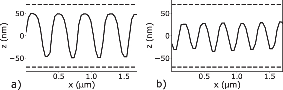
Figures 11(c) and 12(c) depict results obtained from a rectangular silicon grating of 400 nm period and 140 nm height difference (Simetrics RS-N standard). The grating structure is well-resolved in the interferograms and 3D FT shows peaks besides the contribution coming from specular reflection. These peaks are related to first order diffraction, as it is discussed in section 4.2. Respective results for a grating period of 300 nm from the same standard are depicted in figures 11(d) and 12(d). The grating structure is hard to recognize in the image stack shown in figure 11(d). However, figure 12(d) reveals first order diffraction maxima at higher qx values compared to figure 12(c). Due to the transfer characteristic these are further damped, such that the reconstructed profile according to figure 13(b) shows a lower amplitude compared to the profile obtained for the grating of 400 nm period according to figure 13(a).
Figure 13. Reconstructed profile of 400 nm period length (a) and 300 nm period length (b). The evaluation wavelength  amounts to
  nm for the first and
  nm for the latter case, the dashed horizontal lines represent the nominal height of the gratings.
Download figure:
Standard image High-resolution image
Note, that in order to obtain a maximum grating amplitude for the grating of 400 nm period an evaluation wavelength of 610 nm was chosen, whereas for the 300 nm grating an evaluation wavelength of 720 nm is used. In both cases according to (36) the evaluation wavelength corresponds to the qz -value of the diffraction peaks in figures 12(c) and (d) and they are significantly longer than the equivalent wavelength of the CSI signals of 580 nm. Since the profile reconstruction is based on the zeroth and first order diffracted light only, a sinusoidal course of the reconstructed profiles appears, although the original shape of profile is rectangular. In general, even sinusoidal phase gratings show multiple diffraction orders, but if the spatial frequency of a grating approaches the maximum transit frequency of the optical system (see equation (35)) the surface will be reconstructed using only the first diffraction order. However, a good fidelity of the reconstructed grating surface requires that the most dominant diffraction orders contribute to the image formation. Obviously, this requirement is not fulfilled for the grating structures shown in figure 13. Nevertheless, surface features such as the grating period can still be gathered.
More detailed measurement results of different surface structures including the surface of a Blu-ray disc are reported in previous papers [38, 39].
5.3. Spherical surface
Finally, a steel sphere of approximately 6 µm diameter was measured in order to confirm the overall shape of the 3D TF. Figure 11(e) shows the interference fringes. The contributions of the flat base visible to the left and to the right of the sphere were suppressed and the corresponding cross section of the 3D FT result is displayed in figure 12(e). Apart from small deviations, which have to do with the imperfections of the surface of the sphere and maladjustments as well as aberrations of the measuring instrument, the outer shape of the TF can be clearly recognized. The intensity originating from specular reflection at the top of the sphere is located at qx = 0 and dominates compared to other contributions. If steeper flanks of the measured sphere are to be obtained from the results the evaluation wavelength needs to be increased. This is a consequence of qz -values, which decrease on average as the tilt angle and therefore the corresponding qx -values increase.
6. Conclusion
In this contribution a modified CSI model called the double foil model is introduced, which is a combination of both Kirchhoff's diffraction theory and Abbe's theory of image formation in a microscope. The surface of the object under investigation may be mathematically treated either based on the foil model or as a phase object. The scattering process assuming incoherent illumination is described by use of an Ewald sphere allowing to determine the transfer function of a CSI instrument depending on its NA. In contrast to other models the reference and the object wave in a CSI instrument are treated in the same way, enabling the model to be extended to tilted surfaces or reference surfaces of different geometry.
Since elastic light scattering occurs, the length of the wave vectors of incident, reflected, diffracted and scattered light are constant and, therefore, the coordinate values of the transfer function in the 3D spatial frequency domain are not independent of each other. As a consequence, describing the 3D response of a CSI instrument by a linear filtering approach in form of a 3D convolution of the foil representation of the surface and a single 3D PSF resulting from 3D Fourier transformation of the transfer function of the instrument does not hold in general. It leads to a similar approximation of the transfer characteristics as the use of a single equivalent wavelength in signal analysis. Especially for higher NA objective lenses these approximations fail as the PSF changes depending on the features of the measurement object such as surface slope and relevant surface spatial frequency contributions.
In contrast, the double foil model corresponds quite well to both theoretical considerations and experimental findings. Even for rectangular phase gratings, which typically do not fulfill the prerequisites of Kirchhoff's diffraction theory the basic transfer behavior can be derived.
Both theoretical and experimental results confirm that the full lateral resolution capabilities of an interference microscope and the maximum surface slope measurement capability require a proper adaption of the signal evaluation wavelength, which needs to be chosen generally longer compared to the so-called equivalent wavelength.
Acknowledgments
The support of this research work by the German Research Foundation (DFG) under Nos. LE992/13-1, 14-1 is gratefully acknowledged.