


Introduction
Glaciers are important indicators of climate change (Oerlemans, Reference Oerlemans2001; WGMS, 2008; Roe and others, Reference Roe, Baker and Herla2017). In response to global atmospheric warming, glaciers experienced a world-wide retreat and a strong mass loss (Pörtner and others, Reference Pörtner, Mintenbeck, Alegria, Nicolai, Okem, Petzold, Rama and Weyer2019; Zemp and others, Reference Zemp2019). The current observed mass loss of glaciers in the two large Central Asian mountain ranges, the Tien Shan and the Pamir, is furthermore strongly impacting the runoff regimes of the two large river systems, Amu Darya and Syr Darya (Krasznai, Reference Krasznai, Xenarios, Schmidt-Vogt, Qadir, Janusz-Pawletta and Abdullaev2019; Pritchard, Reference Pritchard2019). Model projections for these rivers show that peak runoff is expected in this region in the middle of the century (Huss and Hock, Reference Huss and Hock2018). Afterwards, a strong decline in water availability is expected until the end of the century. The expected runoff changes would affect people's livelihood downstream from the glacierised mountain ranges as meltwater from the glaciers is a major freshwater contributor to the total river runoff (Armstrong and others, Reference Armstrong2019). A reduction of this resource might furthermore contribute to political instabilities (Bernauer and Siegfried, Reference Bernauer and Siegfried2012; Krasznai, Reference Krasznai, Xenarios, Schmidt-Vogt, Qadir, Janusz-Pawletta and Abdullaev2019).
In Central Asia, time series of in situ glaciological measurements are sparse and often discontinuous. Nevertheless, these direct measurements provide an essential source of data for assessing local and regional glacier changes (Hoelzle and others, Reference Hoelzle2017). Direct glaciological measurements are complemented by remotely sensed geodetic glacier changes, i.e. repeated measurements of glacier surface elevation (e.g. Kronenberg and others, Reference Kronenberg2016).
Only geodetic glacier mass balances can be derived for entire mountain ranges. Glaciological mass balance generally benefit from cross validation against geodetic estimates. There exists a considerable amount of region-wide to catchment or glacier specific geodetic measurements of glacier changes in Central Asia for the recent two decades (e.g. Gardelle and others, Reference Gardelle, Berthier, Arnaud and Kääb2013; Brun and others, Reference Brun, Berthier, Wagnon, Kääb and Treichler2017; Shean and others, Reference Shean2020). Some of these studies cover periods of several decades (Aizen and others, Reference Aizen, Kuzmichenok, Surazakov and Aizen2006, Reference Aizen, Kuzmichenok, Surazakov and Aizen2007; Surazakov and Aizen, Reference Surazakov and Aizen2010; Lambrecht and others, Reference Lambrecht, Mayer, Aizen, Floricioiu and Surazakov2014; Holzer and others, Reference Holzer2015; Pieczonka and Bolch, Reference Pieczonka and Bolch2015; Goerlich and others, Reference Goerlich, Bolch, Mukherjee and Pieczonka2017). These geodetic measurements of glaciers rely on declassified spy imagery that is photogrammetrically processed to produce digital elevation models (DEMs). Accuracy in such DEMs, however, generally does not reach the resolution and precision of DEMs from aerial photographs. Studies based on high-resolution and high-quality imagery are thus needed as reference. So far, no long-term geodetic glacier change estimate is available for glaciers located in the Pamir-Alay.
Geodetic surveys of glacier volume and mass change depend on the availability of DEMs. Today, spaceborne data provide a large pool of data for DEM acquisition. Before the onset of the satellite era, DEMs have been derived by means of terrestrial or aerial stereo photogrammetry (Finsterwalder, Reference Finsterwalder1954). In recent years, with advances in 3-D computer vision algorithms and hardware improvements, Structure from Motion (SfM) photogrammetry has gained popularity and found numerous applications in Geosciences (Smith and others, Reference Smith, Carrivick and Quincey2015; Carrivick and others, Reference Carrivick, Smith and Quincey2016). Although traditional stereo photogrammetry requires metadata information about the calibration of cameras and ground control information, SfM only requires numerous overlapping 2-D images for input which can later be georeferenced using ground control information (Lowe, Reference Lowe2001; Westoby and others, Reference Westoby, Brasington, Glasser, Hambrey and Reynolds2012; Micheletti and others, Reference Micheletti, Chandler, Lane, Cook, Clarke and Nield2015). Various authors have applied ground-based SfM to derive high-resolution DEMs of glaciers and to calculate geodetic volume changes and mass balances (e.g. Piermattei and others, Reference Piermattei, Carturan and Guarnieri2015, Reference Piermattei2016; Marcer and others, Reference Marcer2017), yet SfM has not extensively been applied to process historical aerial imagery acquired over steep, mountainous terrain and on glaciers. Girod and others (Reference Girod, Ivar Nielsen, Couderette, Nuth and Kääb2018) used oblique imagery acquired in 1936 to derive high-resolution and high-quality elevation data over glaciers in Svalbard. Mölg and Bolch (Reference Mölg and Bolch2017) evaluated surface elevation changes over the tongue of Zmuttgletscher in Switzerland on DEMs created from aerial imagery between 1946 and 2005. Mertes and others (Reference Mertes, Gulley, Benn, Thompson and Nicholson2017) derived high-resolution glacier DEMs from archival imagery but did not study glacier volume or mass changes. SfM bears a large potential to calculate DEMs for the early or pre-satellite era. Where the quality and availability of the aerial imagery is good, SfM allows generating DEMs that might serve as reference data sets for other studies.
Here, we used Soviet-era aerial photographs in combination with SfM photogrammetry to produce a 4 m resolution DEM of Abramov Glacier for the year 1975. In combination with recent high-resolution elevation data from Pléiades (Gleyzes and others, Reference Gleyzes, Perret and Kubik2012; Berthier and others, Reference Berthier2014), we performed a detailed assessment of volume and mass change of Abramov Glacier located in the Pamir-Alay range. The high detail of the aerial photographs allowed for computation of an accurate DEM for a time period where previously no such data existed. We put our results in context with local and regional geodetic mass-balance estimates.
Study area and data
Abramov Glacier
Abramov Glacier is a valley glacier in the Pamir-Alay range in Kyrgyzstan, Central Asia. The glacier drains into the Koksu river and lies in the head watershed of Vakhsh river flowing south-westwards into the Amu Darya River Basin (Fig. 1).
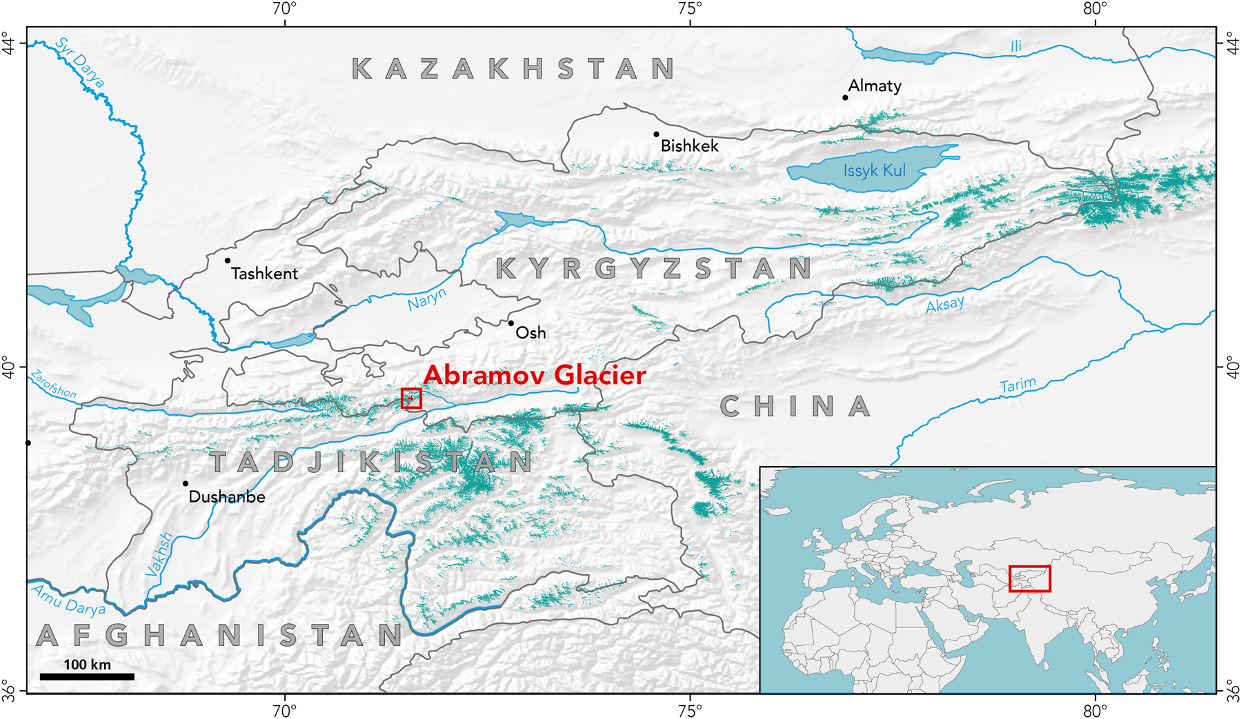
Fig. 1. Overview map of glaciation (turquoise) in Central Asia. The study site, Abramov Glacier, is located in the red box. Source data from Natural Earth (http://www.naturalearthdata.com). Glacier extent source data: RGI version 6.0 (RGI, 2017).
Abramov Glacier features an abundance of glaciological in situ data because a research station was built in 1967 by the Central Asian Research Hydrometeorological Institute. The research station delivered continuous mass-balance observations from 1968 to 1999. The break-up of the former Soviet Union led to a lack of funding and the monitoring programme was interrupted in 1999 when the research station was attacked and destroyed (WGMS, 2001). In 2010/11, the monitoring of several glaciers in Central Asia, including Abramov Glacier, was re-initiated (Hoelzle and others, Reference Hoelzle2017, Reference Hoelzle, Xenarios, Schmidt-Vogt, Qadir, Janusz-Pawletta and Abdullaev2019).
From 1850 to 2015, a retreat of the glacier tongue of ~2 km has been observed (WGMS, 2017). Barandun and others (Reference Barandun2015) report a retreat of the glacier tongue of ~1 km from 1975 to 2015 and an area reduction of 5%. Abramov Glacier advanced by ~400 m between 1972 and 1973. The event was monitored in a very detailed manner and is considered a surge (Emeljyanov and others, Reference Emeljyanov, Nozdryuhin and Suslov1974; Suslov and others, Reference Suslov1980; Glazirin and others, Reference Glazirin, Kamnyanski, Mazo, Nozdryukhin and Salamatin1987, Reference Glazirin, Kamnyanski and Pertziger1993; Glazirin and Braun, Reference Glazirin and Braun2005).
Kuzmichenok and others (Reference Kuzmichenok, Vasilenko, Macheret and Moskalevskiy1992) report an area of 23.3 km2 for the year 1986. They report a mean ice thickness of 110 m and a maximum ice thickness of 247 m derived by radio echo soundings. They estimated a total glacier volume of 2.57 km3.
Barandun and others (Reference Barandun2015) re-analysed the mass-balance data for the years 1968–98 based on field measurement data and modelled the mass balance for the period of missing field data between 1995 and 2011. Combining modelled and re-analysed data, they reported a mean specific mass balance of − 0.44 ± 0.10 m w.e. a −1 for 1968–2014 (Barandun and others, Reference Barandun2015). Barandun and others (Reference Barandun2018) report a mean specific geodetic mass balance of $-0.39 \pm 0.16{\, \rm \, m\, w.e.\, a^{-1}}$ for 2003–2015.
Aerial imagery
Historical aerial photographs acquired during the time of the Soviet Union were available for this study (Mandychev and others, Reference Mandychev, Usubaliev and Azisov2017). The aerial imagery was acquired with a Soviet camera AFA-TES system developed in the late 1940s. The camera system featured a Russar 63V lens with aperture values ranging from f/6.8 to f/16 and shutter speeds ranging from 1/70 s to 1/850 s (Iljin, Reference Iljin1969). The focal length was 101.39 mm. The flying altitude was 3800 m above ground and results in a scale of 1:32 000. The images are panchromatic and overall of good quality. We did not acquire the original aerial images but instead obtained contact prints of size 18 cm × 18 cm. For the year 1975, the whole glacier area is covered by the flight tracks. The along-track overlap is ~70% and cross-track overlap amounts to ~45%. For 1975, a total of 23 aerial photographs were used for analysis. The target imagery was acquired in mid July 1975 and not at the end of the ablation season; some snow is present on the glacier surface. The upper part of the accumulation area features low texture details and low contrast which can challenge SfM processing (Micheletti and others, Reference Micheletti, Chandler, Lane, Cook, Clarke and Nield2015). Due to their age the prints show moderate signs of wear and tear such as artificial scratches but the glacier surface is not affected.
Satellite stereo images and Pléiades DEM
A total of three pairs of Pléiades stereo images (Berthier and others, Reference Berthier2014) were acquired over Abramov Glacier on 20th August 2015 and 1st September 2015 (Fig. 2). From this, two DEMs with a spatial resolution of 4 m were created using the open-source software Ames Stereo Pipeline (Shean and others, Reference Shean2016). The panchromatic and the four multi-spectral channels of the Pléiades satellite were used to compute the DEM. Although they have a coarser resolution, the multi-spectral channels were added in the processing as they were less saturated than the panchromatic channel. This approach reduced the area of voids in the accumulation area. This DEM, DEM 2015, was used as a reference. Data voids of the DEM 2015 amount to a total of 0.64 km 2 (2.6% of the total glacier area) and are mainly found in the accumulation area. The DEM 2015 was generated in WGS84 and set to UTM zone 42 North. Altitudes are defined above the EGM96 geoid. The standard deviation over stable terrain can be used as a measure of accuracy if a reference DEM is available (Fisher and Tate, Reference Fisher and Tate2006).
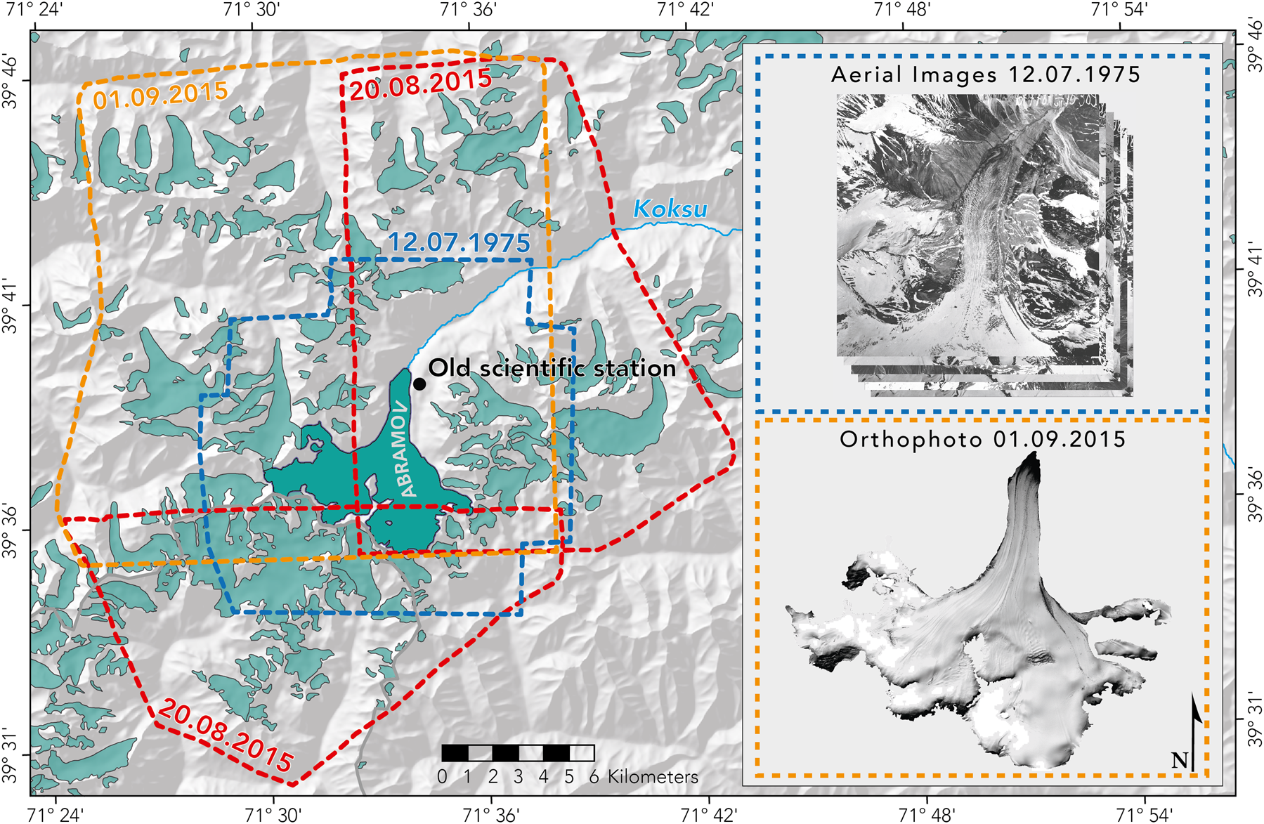
Fig. 2. Overview map of Abramov Glacier with footprints of the 2015 Pléiades stereo-pairs (red and orange dotted lines) and aerial imagery coverage of 1975 (blue dotted line). Glacier area derived from RGI 6.0 are illustrated in turquoise. The SRTM DEM (Farr and others, Reference Farr2007) serves as shaded relief.
We used the DEM and orthoimagery of 1st September 2015 in the subsequent analyses, despite a snow-covered tongue. Fresh snow was not corrected for, even though present on the reference DEM 2015. The snow cover on DEM 2015 was not considered in the uncertainty calculation as it was small (i.e. an estimated 10–30 cm of snow and too small to be quantified by comparing the two Pléiades DEMs from directly before and after snowfall) and its influence on geodetic mass balance is negligible (estimated to be <$1{\, \rm \, cm\, w.e.\, a^{-1}}$ ). This DEM of 1st September 2015 was already used in Barandun and others (Reference Barandun2018) to calculate geodetic mass balance of Abramov Glacier from 2003 to 2015. The Pléiades stereo pair of 20th August 2015 does not cover the entire glacier area of Abramov Glacier, but was used for glacier outline delineation.
Ground control measurements
Ground control measurements on ten reference points located on crests and summits around the glacier were performed during the field seasons of 2014 and 2015. A Topcon dGPS (Topcon GB-1000 receiver with PG-A1 antenna) was used in 2014 and measurements in 2015 were performed with a Trimble device (Trimble 5700 GPS and Trimble R8 GNSS receiver). Furthermore, during the acquisition phase of the Pléiades stereo pairs in late August 2015, 7649 GPS track points were recorded on the glacier. Location measurements from a permanently installed GPS receiver (~1.5 km from the glacier tongue) were used for differential correction of the measured GPS points of both years. The precision of the measured points is 2–3 cm.
Methods
The Abramov archival imagery was processed using the open-source photogrammetric pipeline MicMac (Rupnik and others, Reference Rupnik, Daakir and Pierrot Deseilligny2017). Our SfM workflow is visualised in Figure 3 and follows the recommendations by Girod and others (Reference Girod, Ivar Nielsen, Couderette, Nuth and Kääb2018). Using MicMac has the main advantage of having control over intermediary steps and quality parameters in the processing chain which commercial SfM software often does not permit (Jaud and others, Reference Jaud2016).
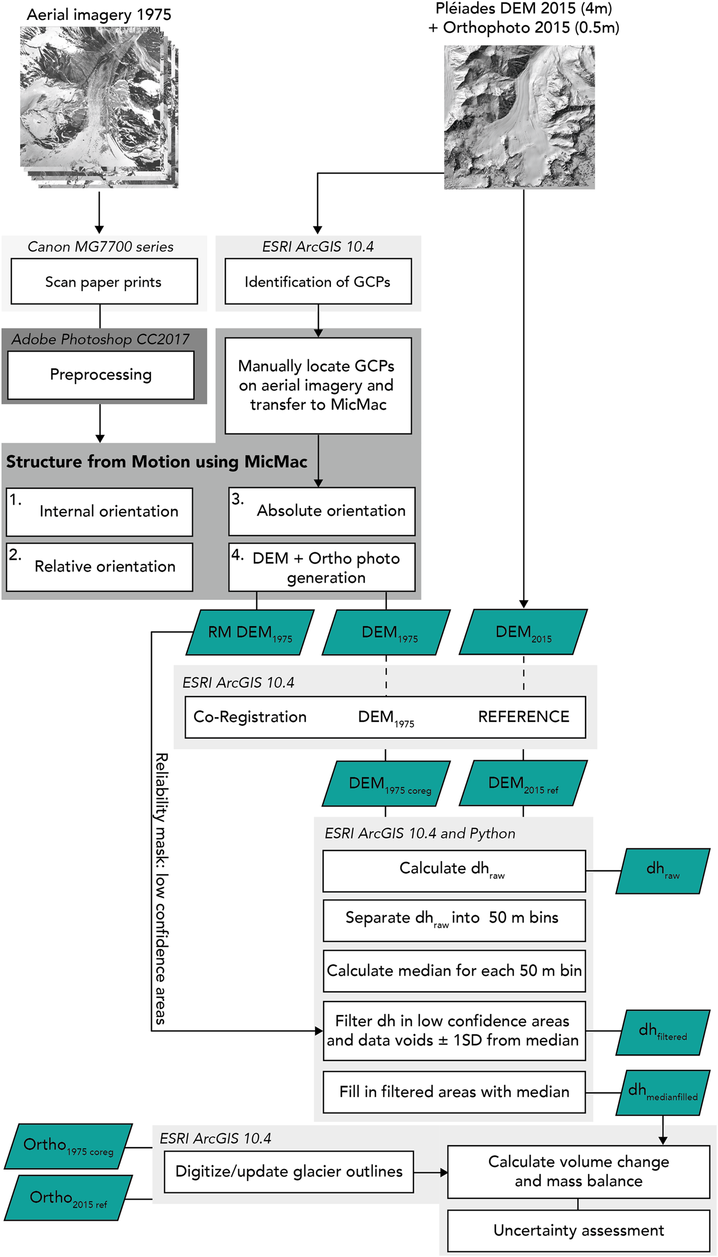
Fig. 3. Workflow of SfM processing pipeline applied in this study, RM stands for reliability mask. Outputs are illustrated in turquoise.
Scanning imagery and internal orientation
The contact prints of size 18 cm × 18 cm were scanned at varying resolutions of 11 μm (2400 dpi) to 21 μm (1200 dpi) as 16 bit TIFF images for the purpose of SfM processing. The scanner model was a commercial scanner model (Canon MG7700 series) which resulted in a ground sampling distance of 89 cm per pixel. All aerial imagery was visually checked for apparent scanning errors such as blurring induced by not equally pressing the image on the scanning plate or different levels of contrast due to faulty scanning properties. Images were pre-processed in Adobe Photoshop. All four corner grid markers were highlighted with a small identification mark. In case the corner grid markers were located in very dark or very bright parts of the imagery and not clearly identifiable, we drew lines through the reseau crosses and reconstructed the corner grid mark position (Fig. 4).
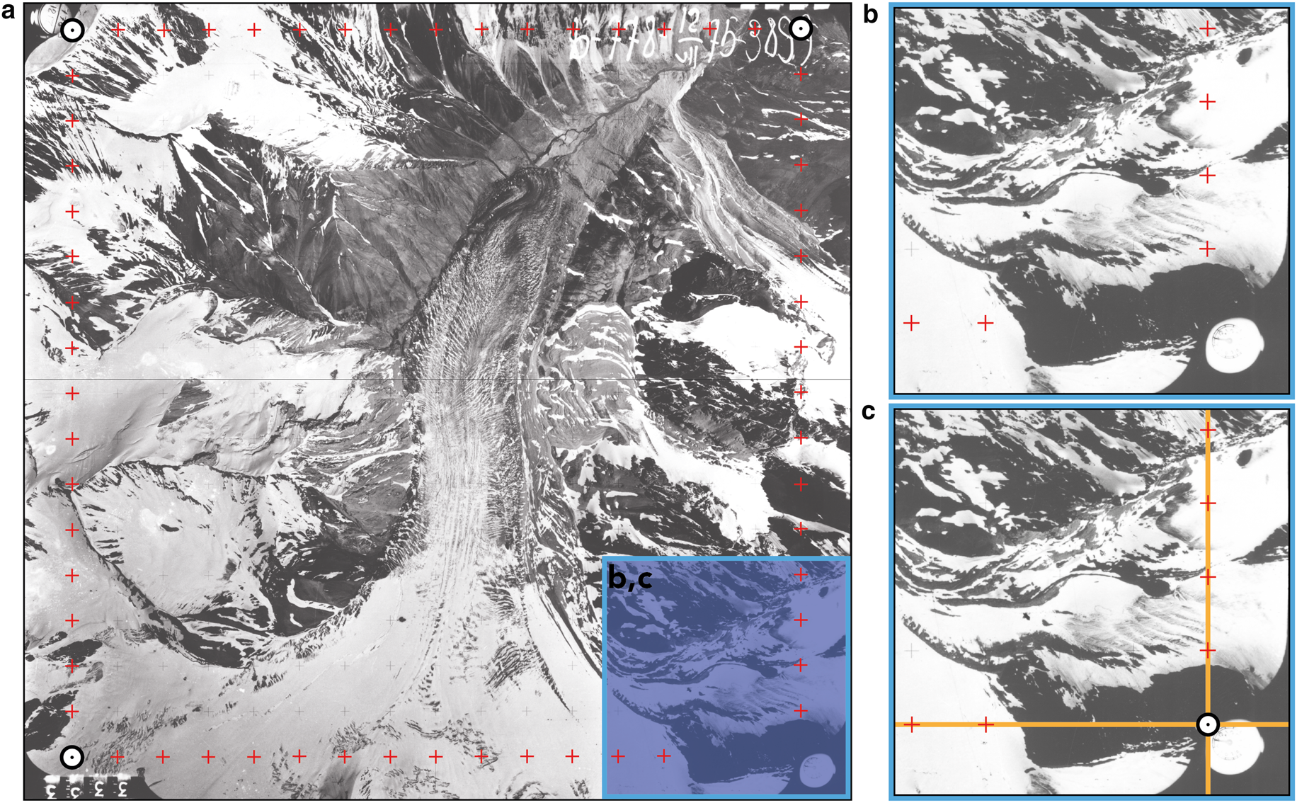
Fig. 4. Example of aerial image pre-processing: reseau crosses on the aerial imagery are highlighted in red. The corner grid markers are marked manually (white dot), however the corner grid marker on the lower right was difficult to place because of shadows in the imagery. Inset b shows a zoom of the lower right corner of a. Inset c shows the applied reconstruction method by drawing two lines (orange) through the reseau crosses which allowed us to find the position of the corner grid mark.
The scanning process can result in slightly different image dimensions and introduce distortions, and thus the interior orientation needs to be standardised (Girod and others, Reference Girod, Ivar Nielsen, Couderette, Nuth and Kääb2018). As no calibration data of the corner grid marker position was available, their relative positions were measured manually and identified on each image. Iljin (Reference Iljin1969) specified the distance in between the reseau crosses on the film as 10 mm. The images were then transformed and resampled to a virtual resolution in a standardised geometry using the MicMac command ReSampFid.
Relative orientation
Tie points on the overlapping images with different acquisition angle were identified in a next step. A total of 253 638 tie points were found for all images using the MicMac command Tapioca. The bundle adjustment estimates the camera location, intrinsic and extrinsic parameters of the camera and outputs a sparse point cloud. This step involves the actual process referred to as SfM: non-linear cost functions are solved to optimise the bundle of projection rays that connect the cameras with the 3-D points and estimate the orientation and internal parameter of the camera (Lowe, Reference Lowe2001).
The known focal length of 101.39 mm and the image size of 18 cm × 18 cm served as an additional input in the calibration estimation. The calibration using the radial lens model Fraser Basic (cf. Pierrot-Deseilligny, Reference Pierrot-Deseilligny2015) was initiated by using the MicMac command Tapas and the focal length was set to a fixed value in order to facilitate a stable calibration. Tapas obtained a residual error of 1.5 pixels.
Absolute orientation and creation of DEM and orthoimage
The orientation is transformed from an arbitrary one into an absolute reference system by georeferencing. The use of ground control points (GCPs) ensures an optimal absolute orientation. GPS field measurements from the end of ablation season 2014 and 2015 were mostly located in very steep terrain or in low contrast areas and not easily identified due to lower resolution of the 1975 imagery. Therefore, it was decided to use the Pléiades orthoimage and DEM as a reference to collect GCPs (Papasodoro and others, Reference Papasodoro, Berthier, Royer, Zdanowicz and Langlois2015; Belart and others, Reference Belart2019). The criteria for the GCP selection was stability over time and an homogeneous distribution over the area of interest (James and Robson, Reference James and Robson2012). Furthermore, clear identification needs to be possible on both the reference and target imagery. To limit the uncertainty of GCP placement, large round and flat boulders and bedrock features of sizes ranging from 5 to 10 m in diameter were favoured. A set of 18 GCPs was manually identified and used to perform the absolute orientation (Fig. 5). The uncertainty of GCP placement was estimated to be 3 pixels.
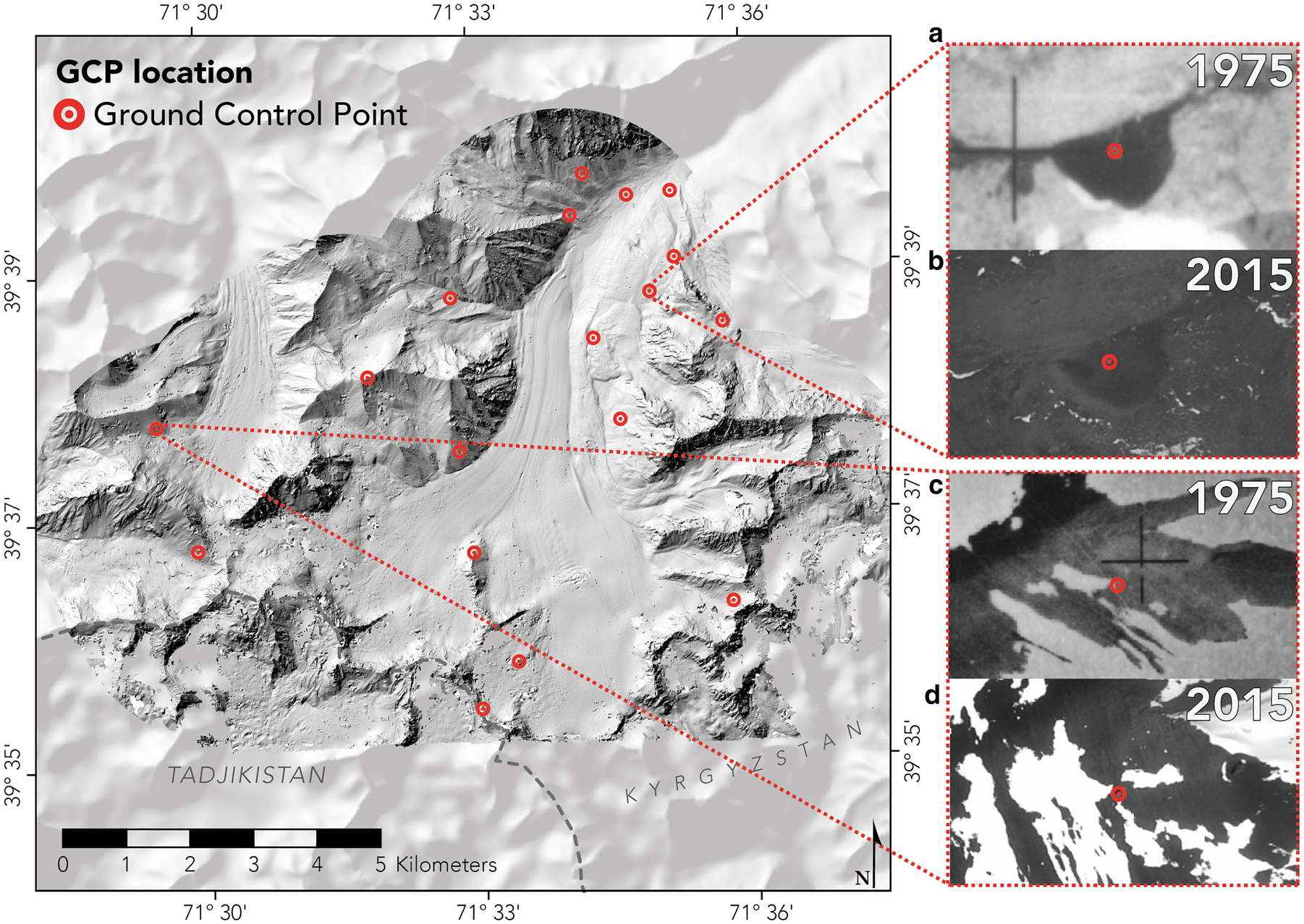
Fig. 5. Locations of GCPs for georeferencing. The small insets on the right show close ups of two GCPs and the corresponding orthoimagery. The GCP location on the aerial imagery 1975 is shown in a and c and the GCP placement of 2015 is shown in b and d. A shaded relief image of the Pléiades DEM from 2015 and the SRTM DEM (Farr and others, Reference Farr2007) serve as background.
Using these GCPs, the model of the 3-D geometry is refined by rerunning the bundle adjustment using the MicMac tool Campari. A dense 3-D point cloud is created using semi-global image matching algorithms with the MicMac command Malt Ortho. Malt Ortho is optimised for matching the images into a regular grid in the ground geometry of the orthoimages (Rupnik and others, Reference Rupnik, Daakir and Pierrot Deseilligny2017). The image matching was performed using an 11 × 11 pixel moving window. From the image matching a DEM with a resolution of 4 m was produced. Using the MicMac module Tawny, an orthophoto mosaic with a resolution of 0.5 m was generated. The DEM and corresponding orthoimages were projected into the same reference system as the reference dataset from 2015.
Reliability map
The SfM chain in MicMac produces a correlation mask which is a measure for the quality of the terrain extraction process. The values of the correlation mask were normalised to values between 0 and 100 and by setting an empirical threshold of 40 (based on visual interpretation of the DEM and orthoimagery), values over 40 were classified with the label high confidence. Correlation mask values below 40 were classified as low confidence.
Determination of stable terrain and co-registration
Before performing a pixel-by-pixel subtraction between the two DEMs, potential systematic errors introduced by the acquisition or processing technique need to be corrected accordingly (Rolstad and others, Reference Rolstad, Haug and Denby2009; Zemp and others, Reference Zemp2013; Paul and others, Reference Paul2015). The DEMs were checked for horizontal and vertical offsets. This analysis was performed over stable ground.
Abramov Glacier is surrounded mostly by steep and potentially moving terrain and the demarcation of stable terrain proved to be difficult. Terrain with slope angle lower than 20° was extracted in the 2015 reference DEM. The glacier areas derived from the Randolph Glacier Inventory (RGI) version 6.0 (RGI, 2017) were excluded. The remaining area was classified as non-moving terrain. The final stable terrain used for co-registration covers an area of 14.3 km 2.
Here, we applied the well-established co-registration approach of Nuth and Kääb (Reference Nuth and Kääb2011). It provides a robust solution for co-registration also in cases when stable terrain is limited to <10% of the scene (Nuth and Kääb, Reference Nuth and Kääb2011). The 2015 DEM served as a reference, therefore it was important to assess its absolute accuracy. As expected, due to the use of GCPs, no large shift was observed by applying this co-registration method. We shifted the DEM and corresponding orthoimagery by the vectors of 0.1 m in the x direction, 6.0 m in the y direction and 0.0 m in the z direction. The standard deviation of vertical differences across stable terrain between the 1975 and the 2015 DEMs after co-registration was 43.2 m.
Delineation of glacier outlines
Glacier outlines were digitised based on the orthophotos of 1975 and 2015. Glacier outlines based on Landsat imagery from Barandun and others (Reference Barandun2018) served as an additional cross-reference in the digitising process. The Pléiades stereo-pairs of 20th August 2015 exhibited less fresh snow and were used to delineate glacier outlines. The area derived from Landsat outlines (Barandun and others, Reference Barandun2018) differs from our digitised outlines by 4.7% (1975) to 1.4% (2015) respectively, which is likely a conservative estimate of the uncertainty of our glacier delineation as we worked with high-resolution imagery. Our estimate agrees well with previously published area uncertainty estimates for high-resolution datasets (Paul and others, Reference Paul2013).
Accuracy assessment of DEM 2015
The horizontal and vertical accuracy of the reference DEM 2015 was assessed by comparing dGPS field measurements in 2014 and 2015 against the horizontal and vertical position of the DEM 2015 off-glacier and on-glacier.
For a total of ten dGPS points off-glacier, the mean of the differences in the x direction (0.51 ± 0.99 m (1σ)), y direction (− 1.24 ± 0.72 m (1σ)) and z direction (0.03 ± 4.03 m (1σ)) were calculated. Additionally, a total of 7649 GPS track points acquired during the field campaign from 24th August to 27th August 2015 were analysed on-glacier in order to get a comprehensive assessment of the vertical DEM accuracy. A mean of difference in elevation of 3.53 ± 1.79 m (1σ)) was found for all points lying on the glacier surface of Abramov Glacier. The data points in the upper part of the accumulation area and near DEM data gaps indicate higher differences between GPS and DEM elevations.
Calculation of thickness change
The SfM-derived DEM 1975 was subtracted from the reference DEM 2015 on a pixel basis in ArcGIS to obtain the thickness change dh map. The values of thickness change were calculated over the glacier surface and divided by the number of years to obtain a mean annual thickness change.
Post-processing: filtering and void filling
Post-processing the dh map was necessary as the image matching process introduced noise and data voids, mostly due to low texture quality in the accumulation area (Fig. 6d). We filtered outliers by binning the thickness change values into 50 m elevation bins and calculating statistical parameters such as mean thickness change, standard deviation and median for each bin. In areas classified as low confidence we excluded values deviating more than one standard deviation from the median in each 50 m bin (Fig. 6e). We then filled these excluded areas with the median calculated for each 50 m elevation bin (Fig. 6f). Median filling was preferred over filling data voids with a mean value, because the median is less susceptible to outliers than the mean (McNabb and others, Reference McNabb, Nuth, Kääb and Girod2019).
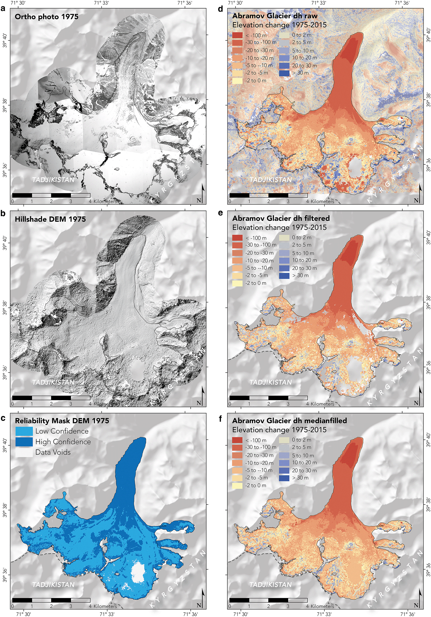
Fig. 6. Data products of DEM 1975: (a) Orthophoto DEM 1975, (b) Hillshade DEM 1975, (c) reliability map DEM 1975, (d) raw elevation change, (e) filtered elevation change and (f) void-filled elevation change. RGI 6.0 outlines are illustrated in blue. The SRTM DEM (Farr and others, Reference Farr2007) serves as shaded relief outside the area of interest.
DEM 1975
The final resolution of the SfM-derived DEM 1975 is 4 m. The on-glacier elevation values are distributed between 3606 and 4969 m a.s.l. Figure 6a–c show the different data products that resulted from the SfM processing within MicMac. The data coverage of the DEM 1975 is 97.4% over the glacier surface. The data voids (2.6%) in the reconstructed DEM 1975 are mainly found in the southeastern tributary of the accumulation area of Abramov Glacier above 4250 m a.s.l. (Fig. 6). Based on the correlation score image in MicMac and the resulting reliability mask pictured in Figure 6c, 44.9% of the glacier pixels were classified as high confidence data, 52.5% as low confidence data and 2.6% are no data values. Low confidence data are predominantly found in the accumulation area (Fig. 6c).
Calculation of volume change and mass balance
Total volume change ΔV in m3 was calculated by using Eqn (1):

where K is the number of pixels covering the glacier at the maximum extent, Δh k is the difference in elevation of the two DEMs at pixel k and r is the pixel size (4 m). The maximum extent in glacier area (1975 for observation period 1975 to 2015) was chosen in order to capture all pixels that were affected by a change in elevation (Koblet and others, Reference Koblet2010).
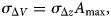
The volume change for the period 1975–2015 was converted into a specific mass balance using Eqn (2):
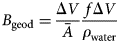
where $\bar {A}$ is the averaged glacier area between the acquisition dates, fΔV is a density conversion factor of 850 kg m −3 adopted from Huss (Reference Huss2013) and ρwater is the density of water (1000 kg m −3). An annual rate of geodetic mass balance B a geod specified in m w.e. a−1 was further calculated by dividing B geod by the number of years n = 40.
Uncertainty analysis
Uncertainties in volume change and mass balance arise from DEM generation such as data voids in low contrast or snow-covered areas (Kääb and Funk, Reference Kääb and Funk1999; Bolch and others, Reference Bolch, Rohrbach, Kutuzov, Robson and Osmonov2019a; McNabb and others, Reference McNabb, Nuth, Kääb and Girod2019).
Random and systematic errors can be introduced during the geodetic calculation of glacier mass changes (Zemp and others, Reference Zemp2013). Here, we estimated only the random error. To assess the uncertainty in the DEMs and errors introduced in the subsequent volume and mass-balance calculation, the uncertainty approach of Fischer and others (Reference Fischer, Huss and Hoelzle2015) was adapted.
A cor in m2 describes a circular area in which errors introduced by the DEM differencing are spatially correlated and is calculated with Eqn (3) adapted from Rolstad and others (Reference Rolstad, Haug and Denby2009):

where L describes the spatial correlation distance in m derived by semivariogram analysis on stable terrain. Within this range, a spatial autocorrelation between two points is established (Rolstad and others, Reference Rolstad, Haug and Denby2009). A spatial correlation length of L = 827 ± 68 m (1σ) was obtained for the observation period 1975–2015. The calculated value for A cor is 2.15 km 2 for 1975–2015.
The uncertainty in surface elevation change on the scale of individual pixels is calculated with Eqn (4) as the correlated area is smaller than the maximum glacier area (Rolstad and others, Reference Rolstad, Haug and Denby2009; Fischer and others, Reference Fischer, Huss and Hoelzle2015):
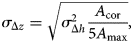
where σΔh in m is defined as the standard deviation over stable terrain (43.2 m). A cor is the correlated area described in Eqn (3) and A max the glacier area at its maximum extent of the observation period (in our case 1975).
The uncertainty in volume change σΔV in m3 is assessed with Eqn (5):
The uncertainty of the geodetic mass balance σgeod in m w.e. is calculated with Eqn (6):
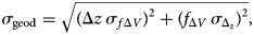
where Δz specifies the mean elevation change in meter, fΔV is a density conversion factor of 850 kg m−3 and σfΔV the corresponding uncertainty in material density of 60 kg m−3 (Huss, Reference Huss2013). σΔz is the uncertainty in surface elevation change derived with Eqn (4).
Results
Changes in glacier area and length
The total glacier area in 1975 was 26.53 km2 of which 1.23 km2 (2.6%) are data voids in the DEM 1975. The total glacier area in 2015 was 24.36 km2. From 1975 to 2015, Abramov Glacier lost 2.17 km2 ($-8.2\percnt$ ) of its surface area. The loss in area was most pronounced at the glacier tongue. The front experienced a retreat of ~1040 m between 1975 and 2015. The relatively small northeastern tributary disconnected from the glacier between 1975 and 2015 and receded ~100 m from 1975 to 2015.
Change in elevation, volume and mass balance from 1975 to 2015
From 1975 to 2015, a mean surface lowering of − 17.03 ± 5.50 m occurred on Abramov Glacier (Fig. 6d). Owing to the ~1 km front position retreat, the lowering is strongest at 3624 m a.s.l. on the tongue, about 1.1 km upstream of the glacier front in 1975. The tongue of Abramov Glacier shows maximum thinning of up to 151.32 ± 5.50 m. A high level of noise (standard deviation outside of glacier area is 81.8 m) is visible in the terrain surrounding the glacier (remarkably in higher regions at the Southern borders of the DEMs, Fig. 6d).
The volume change for 1975–2015 amounts to − 0.45 ± 0.15 km 3. This corresponds to 18% of the glacier volume determined by Kuzmichenok and others (Reference Kuzmichenok, Vasilenko, Macheret and Moskalevskiy1992) in 1986. The calculated mean annual geodetic mass-balance rate for the years 1975 to 2015 is $-0.38 \pm 0.12{\, \rm \, m\, w.e.\, a^{-1}}$ .
.
Figure 6e, f illustrates the result of the void filling approach. In total, 14.8% of the total glacier area was interpolated using the median fill method. Figure 6f shows that an elevation change of close to zero occurred in the accumulation area. Relatively few locations had positive elevation changes (9.8% of the glacier area in 1975; cf. Fig. 6f), generally situated at the uppermost, very steep sections of the glacier. Steep terrain in the accumulation area with low contrast is often associated to high uncertainty in DEMs derived from optical images (Barandun and others, Reference Barandun2018). Mean elevation change in the accumulation area is close to zero, frequent deviations from the mean, including positive values, are related to high levels of noise.
Discussion
Different studies calculated mass balance of Abramov Glacier, however calculations over different time periods challenge a direct comparison (Fig. 7 and Table 1). Only the glaciological measurements exceed the time frame of our estimate, albeit with a large data gap of 16 years. Geodetic mass-balance estimates are only published for the recent period (after the year 2000).
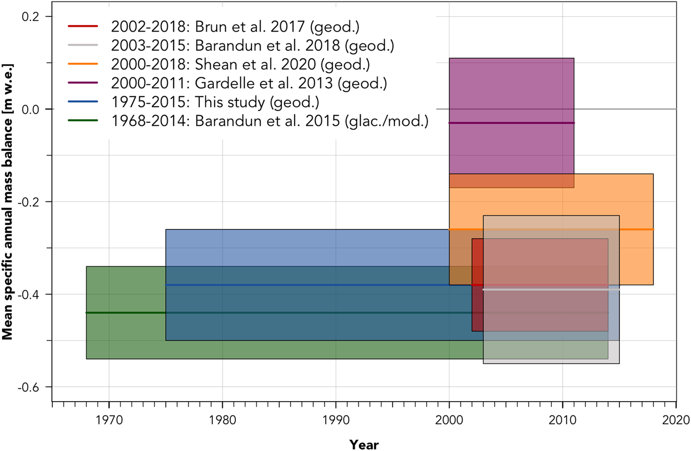
Fig. 7. Mean specific mass balance (geodetic and glaciological/modelled) results for different studies and different time periods for Abramov Glacier. The lines illustrate the mean specific annual mass-balance estimates and boxes display the uncertainty range for the respective publications.
Table 1. Summary of existing glaciological and geodetic mass-balance estimates for Abramov Glacier
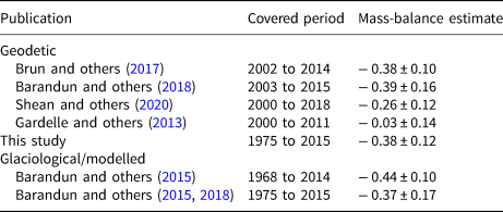
Mass-balance estimates and corresponding uncertainty are specified in m w.e. a−1.
Comparison to other geodetic mass-balance estimates of Abramov Glacier
Brun and others (Reference Brun, Berthier, Wagnon, Kääb and Treichler2017) calculated geodetic mass balance of $-0.38 \pm 0.10{\, \rm \, m\, w.e.\, a^{-1}}$ for the period 2002–2014 using DEMs derived from multi-temporal Advanced Spaceborne Thermal Emission and Reflection Radiometer (ASTER) imagery. Their average annual mass balance is identical to our study ($-0.38 \pm 0.12{\, \rm \, m\, w.e.\, a^{-1}}$
 ). Based on high-resolution Pléiades data (same data source as the reference DEM 2015 used in this study) and Satellite Pour l'Observation de la Terre (SPOT)5 DEMs from 2003 and 2011, Barandun and others (Reference Barandun2018) calculated an average geodetic mass balance of $-0.39 \pm 0.16{\, \rm \, m\, w.e.\, a^{-1}}$
 for the period 2003 to 2015 and $-0.36 \pm 0.26{\, \rm \, m\, w.e.\, a^{-1}}$
 for the period 2011–2015. The same study reconstructed a slightly lower mass loss of $-0.26 \pm 0.20{\, \rm \, m\, w.e.\, a^{-1}}$
 from 1998 to 2016 combining geodetic measurements, numerical modelling, snowline observations and glaciological observations. The dh map in Barandun and others (Reference Barandun2018) shows a pronounced surface lowering mainly on the tongue and almost no change in the accumulation area from 2003 to 2015. Our results show that surface elevation change for the period 1975–2015 in the accumulation area are close to zero. Shean and others (Reference Shean2020) reprocessed thousands of ASTER and very high-resolution imagery (mostly Worldview) DEMs over High Mountain Asia (HMA) from 2000 to 2018. For Abramov Glacier they report a specific annual mass balance of − 0.26 ± 0.12 m w.e. a −1 from 2000 to 2018. The studies of Brun and others (Reference Brun, Berthier, Wagnon, Kääb and Treichler2017) and Shean and others (Reference Shean2020) used stacks of multiple DEMs to derive geodetic mass balance, thus their time stamp is not clearly defined and their results are difficult to compare with a geodetic mass balance derived from only two DEMs (Barandun and others, Reference Barandun2018). Gardelle and others (Reference Gardelle, Berthier, Arnaud and Kääb2013) suggested a mean annual geodetic mass balance of − 0.03 ± 0.14 m w.e. a −1 for Abramov Glacier by differencing SPOT5 imagery from 2011 and SRTM data from 2000. The dh dataset of Gardelle and others (Reference Gardelle, Berthier, Arnaud and Kääb2013) shows significant positive changes of elevation in the accumulation area of Abramov Glacier and at the front of the tongue. Barandun and others (Reference Barandun2018) question the findings of Gardelle and others (Reference Gardelle, Berthier, Arnaud and Kääb2013) and pointed out a possible positive bias in elevation change because of an underestimated penetration of the SRTM X-band radar signal into snow and ice (Dehecq and others, Reference Dehecq2016; Lambrecht and others, Reference Lambrecht, Mayer, Wendt, Floricioiu and Völksen2018).
Overall, our mass balance 1975–2015 is in the same range as mass-balance estimates published for a ~15 years subset (~2000 to 2015: Brun and others, Reference Brun, Berthier, Wagnon, Kääb and Treichler2017; Barandun and others, Reference Barandun2018; Shean and others, Reference Shean2020) of our 40-year time frame (Fig. 7). Thus, we cautiously conclude that mass balance for the two time periods 1975 to ~2000 and ~2000 to 2015 are similar. This would indicate that the rate of mass loss of Abramov Glacier was relatively stable. This assumption is partly confirmed by re-analysis of glaciological measurements (see the following subsection and Barandun and others, Reference Barandun2015) which indicates no general long-term trend in mass balance over the time frame 1968–2014. At this point we can only speculate to why Abramov's rate of mass loss appears to be relatively stable. Kronenberg and others (Reference Kronenberg, Machguth, Eichler and Hoelzlein press) have repeated Soviet firn studies in the accumulation area of Abramov Glacier. The results suggest that accumulation has increased since the 1970s, potentially offsetting increased melt.
Comparison to glaciological and modelled mass-balance estimates
Glaciological mass-balance measurements generally benefit from cross validation against geodetic estimates. Barandun and others (Reference Barandun2015) (re)analysed the glaciological mass balance for the period 1968–1995, 2012–2014 and reconstructed the mass balance from 1995 to 2011. Their mass balance of − 0.44 ± 0.10 m w.e. a −1 from 1968 to 2014 lies in the same range and is valid for a similar time frame as in our study. Re-analysed glaciological measurements (Barandun and others, Reference Barandun2015) in combination with improved modelling (Barandun and others, Reference Barandun2018) provide a mass balance of − 0.37 ± 0.17 m w.e. a −1 from 1975 to 2015. The 1975–2015 area change of 2.17 km 2 and glacier retreat of ~1040 m are in line with the findings by Barandun and others (Reference Barandun2015).
Comparison to regional glacier changes
Considering longer time frames, similar to the one of the current study, Holzer and others (Reference Holzer2015) found a nearly balanced mass-balance budget for Muztagh Ata Glacier basin in the eastern Pamir using declassified spy imagery for the years 1975 to 2013. Using declassified satellite imagery, Zhou and others (Reference Zhou, Li, Li, Zhao and Ding2019) reported an almost balanced mass budget (− 0.03 ± 0.24 m w.e. a −1) between 1975 and 1999 for Central Pamir. Bolch and others (Reference Bolch, P, A, A and AB2019b) reported an averaged mass loss of − 0.26 m w.e. a −1 for the Western Pamir. Barandun (Reference Barandun2018) reported an averaged mass loss of − 0.37 ± 0.42 m w.e. a −1 for the Western Pamir. The results of Pieczonka and others (Reference Pieczonka, Bolch, Junfeng and Shiyin2013) suggest that the overall mass budget of − 0.33 ± 0.15 m w.e. a −1 for 1976–2009 for the glaciers in the Aksu-Tarim catchment further north in the Central Tien Shan lies in the same range as here calculated for Abramov. Our results, together with those from the literature, draw a picture of moderate multi-decadal mass loss (mass balance of typically − 0.2 m to − 0.4 m w.e. a −1) in the Western Pamir, Pamir Alay and Central Tien Shan. The literature furthermore indicates that over a similar time period glacier mass budgets in Central and Eastern Pamir were almost balanced, despite heterogeneous response for individual glaciers within each region (Scherler and others, Reference Scherler, Bookhagen and Strecker2011; Farinotti and others, Reference Farinotti2015; Kääb and others, Reference Kääb, Treichler, Nuth and Berthier2015; Brun and others, Reference Brun, Berthier, Wagnon, Kääb and Treichler2017; Wang and others, Reference Wang, Yi, Chang and Sun2017; Shean and others, Reference Shean2020).
Conclusions
In this study, we derived a DEM and outlines of Abramov Glacier for the year 1975 based on Soviet aerial images. A high-resolution Pléiades DEM acquired in September 2015 served as a reference for the GCPs and for the calculation of area, volume and mass changes between 1975 and 2015. For 1975–2015, there was a reduction of $-8.2\percnt$ in glacier area and a mean annual thickness change of − 0.43 ± 0.14 m a −1. We calculated a mean specific mass balance of − 0.38 ± 0.12 m w.e. a −1. This mass balance is in the same range as glaciological and geodetic mass-balance values published in recent studies for the time period ~2000 to 2015. Calculated mass balance is very similar to the re-analysed glaciological mass balance 1968–2014 of the glacier. In the future, the historic 1975 DEM that we generated from declassified spy imagery could serve as an input for a time series of Abramov Glacier combining all available DEMs, modelled and glaciological mass-balance values. Our results illustrate that SfM is a useful approach for processing historical imagery from Soviet times. Our high-resolution map of elevation change could also help to validate similar estimates using spy satellite imagery.
Acknowledgements
FD, HM, MB, MK, RU and MH acknowledge support by the following organisations: Swiss National Science Foundation (SNSF), grant 200021_155903, German Federal Foreign Office in the framework of the CAWa project (http://www.cawa-project.net), the Swiss Agency for Development and Cooperation (SDC) and the Federal Office of Meteorology and Climatology (MeteoSwiss) through the project Capacity Building and Twinning for Climate Observing Systems (CATCOS) Phase 1 (7F-08114.1) and 2 (7F-08114.02.01), as well as the project CICADA (Cryospheric Climate Services for improved Adaptation, contract no. 81049674) between SDC and the University of Fribourg. HM, MK and MH acknowledge support by SNSF (grant 200021_169453). EB acknowledges support from the French Space Agency (CNES), through the TOSCA and the Pleiades Glacier Observatory (PGO) programmes. All authors wish to thank the editor and the three anonymous reviewers for their valuable comments that led to an improved study.
Author contributions
FD and HM designed the study. FD processed the aerial imagery, performed all calculations and wrote most of the paper, EB provided the DEM 2015 and performed analysis on the GPS data, MB performed analysis on the GPS data. LG provided technical support with MicMac. All authors contributed to writing and revising the paper.


 Open access