
Improved Hybrid Heuristic Algorithm Inspired by Tissue-Like Membrane System to Solve Job Shop Scheduling Problem


1
Business School, Shandong Normal University, Jinan 250358, China
2
Academy of Management Science, Shandong Normal University, Jinan 250358, China
*
Author to whom correspondence should be addressed.
Processes 2021, 9(2), 219; https://doi.org/10.3390/pr9020219
Submission received: 21 December 2020
/
Revised: 20 January 2021
/
Accepted: 21 January 2021
/
Published: 25 January 2021
(This article belongs to the Special Issue Modeling, Simulation and Design of Membrane Computing System)
Abstract
:In real industrial engineering, job shop scheduling problem (JSSP) is considered to be one of the most difficult and tricky non-deterministic polynomial-time (NP)-hard problems. This study proposes a new hybrid heuristic algorithm for solving JSSP inspired by the tissue-like membrane system. The framework of the proposed algorithm incorporates improved genetic algorithms (GA), modified rumor particle swarm optimization (PSO), and fine-grained local search methods (LSM). To effectively alleviate the premature convergence of GA, the improved GA uses adaptive crossover and mutation probabilities. Taking into account the improvement of the diversity of the population, the rumor PSO is discretized to interactively optimize the population. In addition, a local search operator incorporating critical path recognition is designed to enhance the local search ability of the population. Experiment with 24 benchmark instances show that the proposed algorithm outperforms other latest comparative algorithms, and hybrid optimization strategies that complement each other in performance can better break through the original limitations of the single meta-heuristic method.
1. Introduction
The production scheduling system plays a vital role in a specialized manufacturing system. It is the core of technologies that realize the overall management of the manufacturing system, the optimization of target tasks, and the automation of scheduling execution. Under the premise of meeting resource and process constraints, formulating a scientific and reasonable production scheduling plan plays critical role in controlling finished product inventory, shortening the maximum completion period, and optimizing machine load. Job shop scheduling problem (JSSP) is recognized as a very challenging and representative NP-hard problem in scheduling problems [1]. Its application field is extremely wide, involving aircraft carrier dispatching, airport aircraft dispatching, port terminal cargo dispatching, automobile processing assembly line, etc.
Since Fisher and Thomson [2] gave three benchmarks of JSSP in 1963, JSSP has attracted wide attention from many scholars. For more than half a century, many methods for solving JSSP have been proposed. These methods can be roughly summarized into two categories: precise methods and approximate methods. Some early research works focused on precise methods, including branch and bound, mathematical programming [3,4,5] etc. However, these precise methods only tend to solve small-scale problems, and the computational cost on larger-scale problems is unacceptable. As the complexity of JSSPs increases, the excellent performance of some approximation methods has attracted the attention of scholars, including priority dispatch [6], shifting bottleneck procedure [7], and meta-heuristics. Among them, priority dispatch and shifting bottleneck are considered simple heuristics, and they are undistinguished in terms of effectiveness [8]. Different from problem-based simple heuristics, meta-heuristics draw inspiration from some random phenomena in nature and incorporate random factors. These random factors make the algorithm have a certain probability to jump out of the local optimal and try to develop the global optimal solution. Therefore, the problem-independent meta-heuristic algorithms have been widely used in various fields and have shown considerable performance. Meta-heuristic algorithms commonly used to solve JSSP include genetic algorithm (GA) [9], particle swarm optimization algorithm (PSO) [10,11], ant colony optimization algorithm (ACO) [12], simulated annealing (SA) [13], and tabu search (TS) [14], etc.
However, as a classic discrete combinatorial optimization problem, JSSP has its inherent stubborn nature. Whether it is classic GA or PSO, a single meta-heuristic method will always face the problem of premature convergence, and its search performance has reached its limit. Therefore, after entering the 21st century, more and more scholars are devoted to studying hybrid optimization strategies in order to integrate the complementary advantages of different meta-heuristic methods. Zhang et al. [15] proposed a hybrid heuristic algorithm by merging GA and SA. Zhang et al. [16] proposed the famous crossover operator, i.e., precedence operation crossover (POX), and combined the improved GA with the local search algorithm. To better achieve a balance between diversification and intensification, Kurdi [8] merged the island model GA (IMGA) with TS. Abdel-Kader [17] combines standard PSO and GA to solve JSSP. Zhou [18] fuses the social spider optimization algorithm and the differential evolutionary based mutation operator for solving the JSSP. Peng et al. [19] proposed a MAGATS algorithm that combines multi-agent GA and TS to solve JSSP. Pongchairerks [20] presented a two-level meta-heuristic method for solving JSSP, where the upper-level algorithm (UPLA) was a population-based algorithm that serves as an input-parameter controller of the lower-level algorithm (LOLA). Aiming at the JSSP, a collective communication hybrid genetic algorithm using distributed processing is proposed [21].
Membrane systems were formally presented by Păun [22] in 1998. Since then, membrane computing has become an emerging research field in computer science and has attracted a large number of scholars’ research interests due to its outstanding characteristics of distribution, parallelism and non-determinism. Membrane computing aims to explore new computing models from biological cells (especially cell membranes), which is also called membrane system or P system. Membrane system contains three basic components: membrane structure, objects and rules. Up till now, membrane computing models are mainly summarized into three categories, i.e., cell-like P system [22], tissue-like P system [23,24], neural-like P system [25]. In recent years, many other variants of membrane systems have been developed in terms of direct membranes [26,27]. In addition, in the application of indirect membranes, fruitful results have been achieved in the field of combinatorial optimization such as clustering [28,29] and neural networks [30].
Considering the above statement, this work presented a hybrid heuristic algorithm inspired by tissue-like membrane system for solving the JSSP. The algorithm framework combines improved GA, modified PSO, and local search algorithms based on critical paths. Among them, the communication rules between GA and PSO can increase the diversity of the population while delaying premature convergence, and local search can further fine-tune the optimization results. The comparative experiments show that the hybrid algorithm presented in this study outperforms other latest algorithms. Specifically, the contributions of this work are listed below.
- (1)
- A new hybrid heuristic algorithm inspired by tissue-like membrane system is proposed for JSSP. The three types of evolutionary rules of the membrane system are introduced in detail.
- (2)
- Considering to further alleviate the premature convergence of GA, an adaptive crossover and mutation strategy is proposed.
- (3)
- To realize the full exploration of the entire solution space while enhancing the diversity of the population, the rumor PSO algorithm [31] is discretized, making it suitable for solving JSSP which belongs to discrete problem.
- (4)
- Aiming at the results of the above optimization, an algorithm for quickly identifying critical paths is presented. And based on this algorithm, a local search strategy is given.
The remainder of this paper is organized as follow. Section 2 describes the mathematical modeling and disjunctive graph representation of JSSP. Section 3 gives a detailed description of the proposed hybrid heuristic algorithm inspired by the tissue-like membrane system, including three improved sub-algorithms and the rules of the P system. Section 4 reports the results of comparative experiments on several sets of benchmark instances. Section 5 concludes this work with a summary and future research directions.
2. Mathematical Modeling and Disjunctive Graph Representation of JSSP
An JSSP can be formally described as follows. There are jobs and machines denoted as and , respectively. The processing of each job includes operations, and each operation is processed on a designated machine. In other words, the number of machines means the number of operations. There are sequential constraints between different operations of the same job. There is no precedence constraint between different jobs. The operation sequence of each job and its processing time on the corresponding machine are given in advance. The ultimate goal of JSSP is to seek an optimal schedule to minimize the maximum completion time. The number of possible solutions for an JSSP is up to (n!)m. In the process of solving the JSSP, the restrictions or constraints to be followed are described as follows.
- (1)
- At the beginning of processing, any job may be selected for processing.
- (2)
- Once a job starts to be processed on the corresponding machine, no interruption or preemption is allowed.
- (3)
- At a certain moment, a job can only be processed on one machine.
- (4)
- At a certain moment, a machine can only process one job.
- (5)
- Every job must be processed in a predetermined sequence of operations (i.e., the machining paths), which traverses all machines exactly once.
- (6)
- The transportation time generated during processing is not considered.
To facilitate the mathematical modeling of JSSP, the notations used and their meanings are described below.
- (1)
- denotes the j-th operation of the job , where and .
- (2)
- denotes the processing time of .
- (3)
- represents the cumulative completion time of job corresponding to operation .
- (4)
- denotes the earliest cumulative (not including ) start time of the machine corresponding to the operation .
Therefore, considering the above, the mathematical model of JSSP can be formally expressed as follows.
subject to
Equation (1) represents the objective function of JSSP, which is to minimize the maximum completion time, i.e., the makespan. Equation (2) means priority constraints between different operations of the same job. Equation (3) means that preemption on the same machine is not allowed. Equation (4) gives the domains of the variables.
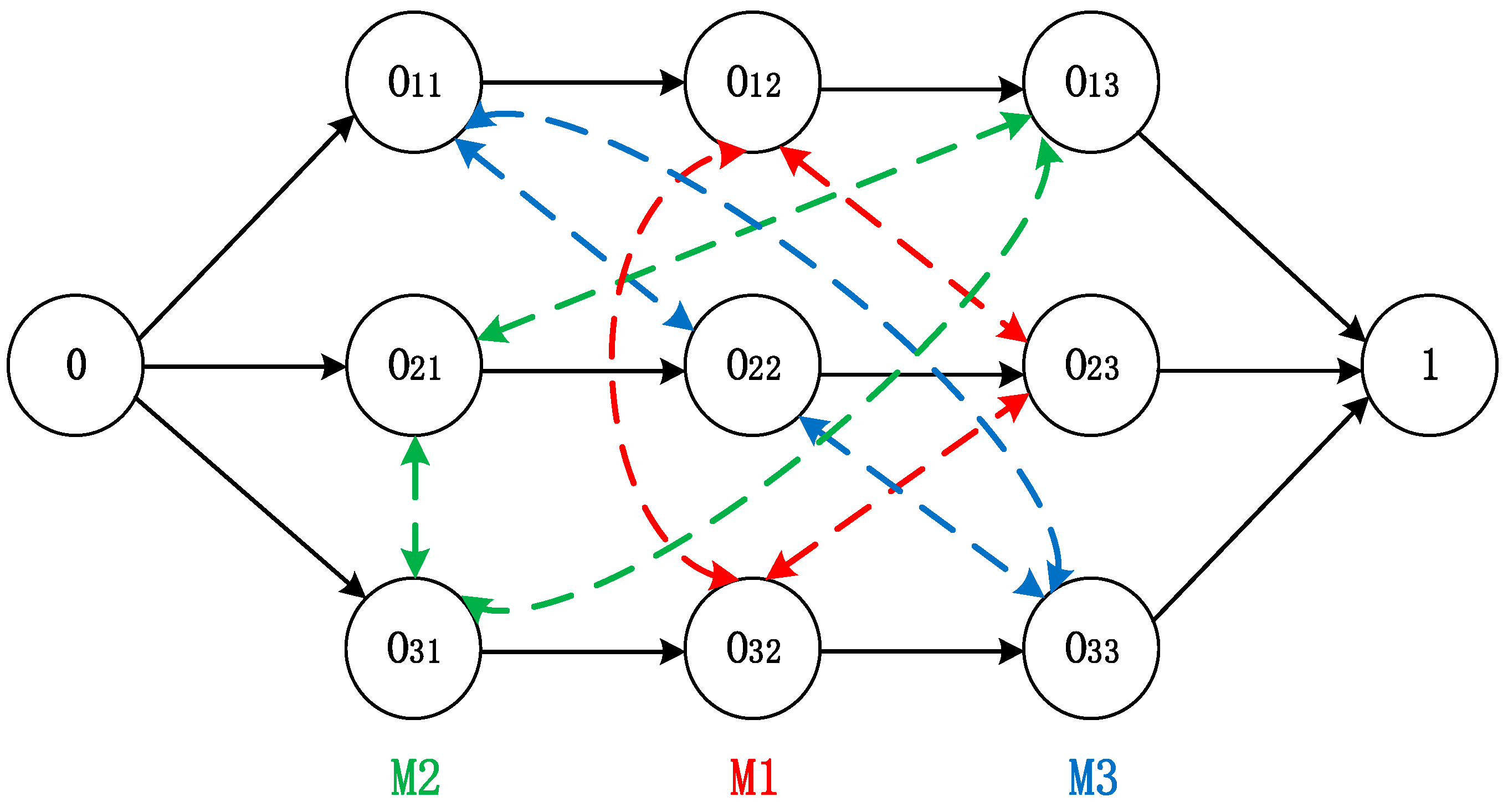
Any JSSP can be intuitively represented by its disjunction graph. Figure 1 shows a disjunctive representation for a JSSP of 3 × 3 (3 jobs and 3 machines). The machine sequence corresponding to the job and the processing time (pij) on the corresponding machine refer to Table 1. The disjunction graph is a triplet G = (V, A, E), where V = {0, O11, O12,…, Onm, 1} means the set of nodes denoting all operations, 0 and 1 represent the virtual start and end nodes, respectively. A represents the set of directed conjunctive arcs, which describes the precedence constraints between different operations on the same job. In Figure 1, the conjunctive arcs are marked with a black solid line, and each of the three rows represents a job, where Oij denotes the j-th operation of the job i. E represents non-directed set of disjunctive arcs, which describes the resource capacity constraints between different operations on the same machine. Specifically, , Where Ek represents a subset of the disjunctive arcs corresponding to machine k. For example, the operations O11, O22, and O33 connected by the disjunctive arcs are all processed on machine 3 (M3). The operations O12, O23, and O32 connected by the disjunctive arcs are all processed on machine 1 (M1). Similarly, the operations O13, O21, and O31 are processed on machine 2 (M2). Assuming that the number of operations processed on the same machine k is n, then the number of disjunctive arcs in the subset Ek is . In other words, the subset Ek is actually a fully connected clique. The dotted lines of different colors in Figure 1 correspond to the disjunctive arcs on different machines.
3. The Proposed Hybrid Heuristic Algorithm Coupling with Tissue-Like P System
This section will describe the tissue-like membrane system coupling with the proposed hybrid heuristic algorithm. The specific content involved includes the structure of the coupled membrane system, the three improved sub-algorithms corresponding to the structure, and the related evolution-communication mechanism.
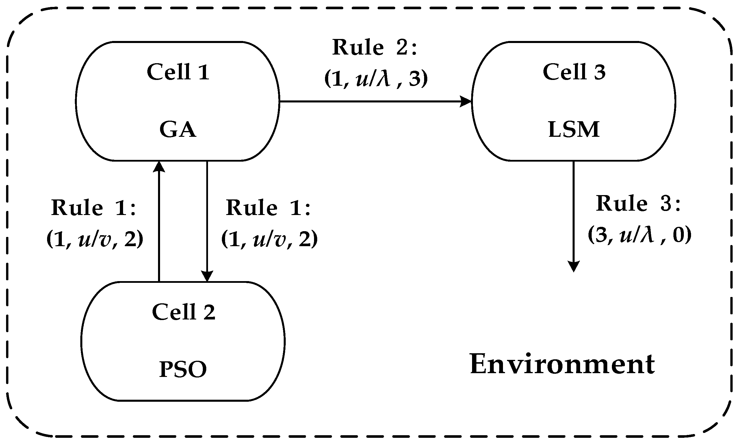
3.1. The Coupled Tissue-Like P System
The cell-like membrane system studies the computer theory of a single cell, while the tissue-like membrane system explores the mechanism by which multiple cells freely placed in the same environment cooperate and communicate with each other to complete calculations. The membrane structure of the tissue-like membrane system is a net structure. Figure 2 shows the membrane structure of the coupled membrane system.
The formal expression of a coupled tissue-like P system with degree 3 is given below.
where:
- (1)
- O is a finite set of non-empty objects, in which the elements, that is, objects, are individuals in the population.
- (2)
- stands for cell, in which there are different objects and evolution rules.
- (3)
- Ri represents the evolution rule corresponding to cell i. Evolution rules are used to improve individuals in a population. The evolution rule is expressed in the form u → v, which means that the object u, that is, the individual in the population, evolves into the object v according to specific rules.
- (4)
- R′ denotes a finite set of communication rules between different cells, which is used to transfer objects between cells, in the form (i, u/v, j), i ≠ j, i, j = 1, 2, 3, .
- (5)
- syn = {(1, 2), (2, 1), (1, 3)} ⊆ {1, 2, 3} × {1, 2, 3} represents the set of channels between cells in the coupled membrane system, as shown by the arcs with arrows in Figure 2.
- (6)
- i0 = 3 means that cell 3 is the output membrane of the coupled P system.
In the above membrane structure, the evolution rules in cell 1, cell 2 and cell 3 are respectively three improved sub-algorithms. The general procedure of the proposed coupled membrane system is described below.
- Step 1:
- The initial population is produced in cell 1, and the initial population size is N. Initially, cell 2 and cell 3 are both empty.
- Step 2:
- The initial N individuals are saved for subsequent evaluation, and their copies are sent to cell 2 according to communication rule 1.
- Step 3:
- The improved GA and the modified rumor PSO are used as evolution rules in cell 1 and cell 2, respectively. Here, the evolution within cell 1 and cell 2 can be regarded as two independent internal loops to improve the initial population.
- Step 4:
- Individuals that have evolved and updated in cell 2 are sent back to cell 1 according to the exchange rule 1. In other words, after reaching the upper limit of the number of internal iterations, 3N individuals will be collected in cell 1.
- Step 5:
- All individuals in cell 1 are sorted in descending order of fitness value and duplicate individuals are removed. According to the elitist strategy, the population size is maintained as N. The resulting N individuals are used as the initialization of the next generation population.
- Step 6:
- The process from Step 2 to Step 5 can be regarded as an external iteration. Repeat steps 2 to 5 until the number of external iterations is met. Then the N individuals finally obtained in cell 2 are sent to cell 3 according to the exchange rule 2.
- Step 7:
- Use the improved local search method (LSM) in cell 3 to improve N individuals. Repeat this step until the termination condition is reached.
- Step 8:
- According to rule 3, the individual with the best fitness value is output to the environment as the final result.
The next few sub-sections will introduce three improved sub-algorithms in detail, which correspond to the evolution rules in the three cells.
3.2. Evolutionary Rule of Objects in Cell 1
The evolutionary rule in cell 1 is the improved GA. This subsection will specifically give the strategies adopted by the improved GA, including encoding and initialization, selection strategies, and adaptive crossover and mutation.
3.2.1. Encoding and Initialization
The existing encoding methods for solving JSSP include job-based, operation-based, and machine-based and so on. Considering the pros and cons of different encoding schemes, operation-based coding is better than others, and it has received the most extensive attention in solving JSSP [19]. For an JSSP, its operation-based encoding method can be expressed as , where represents the job number. The j-th appearance of job i indicates the j-th operation of job i, namely, Oij. Each job number appears exactly m times. Initially, random permutation is performed on the integers from 1 to , and then the sequence is executed element-level modulo n to take the remainder. This ensures that each job number appears exactly m times and forms an operation-based encoding. The advantages of this encoding scheme are:
- The solutions generated during initialization are all feasible solutions.
- Arbitrary arrangement of gene positions in chromosome sequence can still obtain feasible solutions, which is easy for mutation operation.
- Easy to decode.
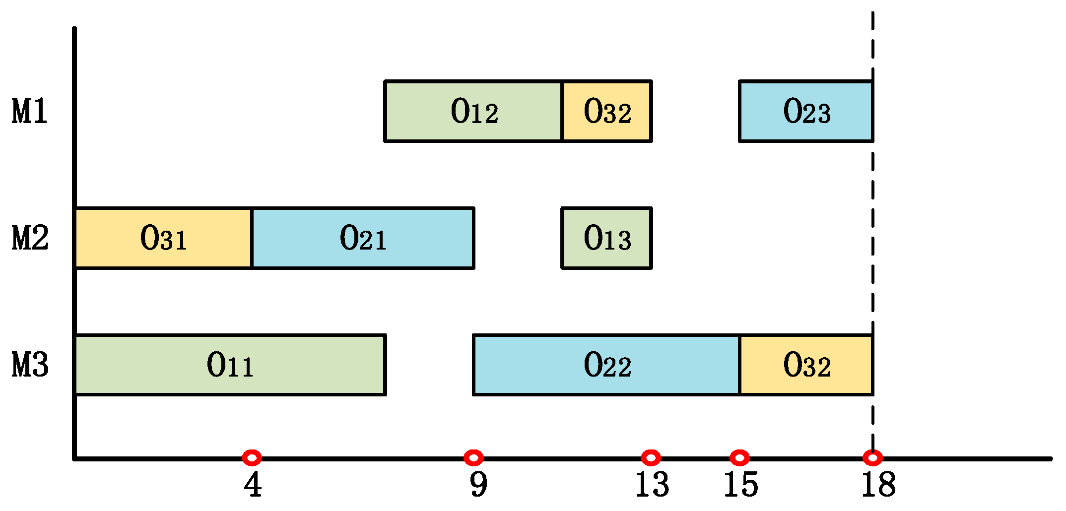
Take the chromosome encoding 1-3-2-2-1-3-3-1-2 of a simple 3 × 3 JSSP as an example, where the machine sequence corresponding to the job and the processing time (pij) on the corresponding machine refer to Table 1. The first number ‘1’ indicates the 1st operation of job 1; the second number ‘3’ means the 1st operation of job 3; the fourth number ‘2’, i.e., the 2nd appearance of job 2, indicates the 2nd operation of job 2. As mentioned above, the i-th appearance of the same job number means the i-th operation of this job. According to the information provided in advance in Table 1, it is easy to decode and calculate the makespan of any encoding sequence. The completion times of jobs 1, 2 and 3 are 13, 18, and 18, respectively. Therefore, the makespan of this chromosome sequence is 18. Figure 3 below shows the scheduling Gantt chart corresponding to this encoding sequence. The same job processed by different machines are identified with the same color.
3.2.2. Fitness Function and Selection Strategy
The fitness function is used to measure the quality of individuals in the population, usually it is a function related to the optimization goal. Taking into account the natural law of “survival of the fittest”, the higher the fitness of the individual, the higher the probability of survival. Therefore, the fitness function in this work is defined as
where x represents an individual in the population.
On the basis of keeping the population size of each generation unchanged, in order to ensure the stable improvement of the overall quality of the population, this work adopts a roulette wheel selection strategy. For any individual xj, the probability P(xj) to be selected is calculated according to the following formula.
When evaluating the fitness of each generation of the population, the elitism strategy is incorporated. This frees the optimal individual from the destruction of operations such as crossover and mutation, and directly replaces the worst individual in the next generation.
3.2.3. Adaptive Crossover and Mutation Operation
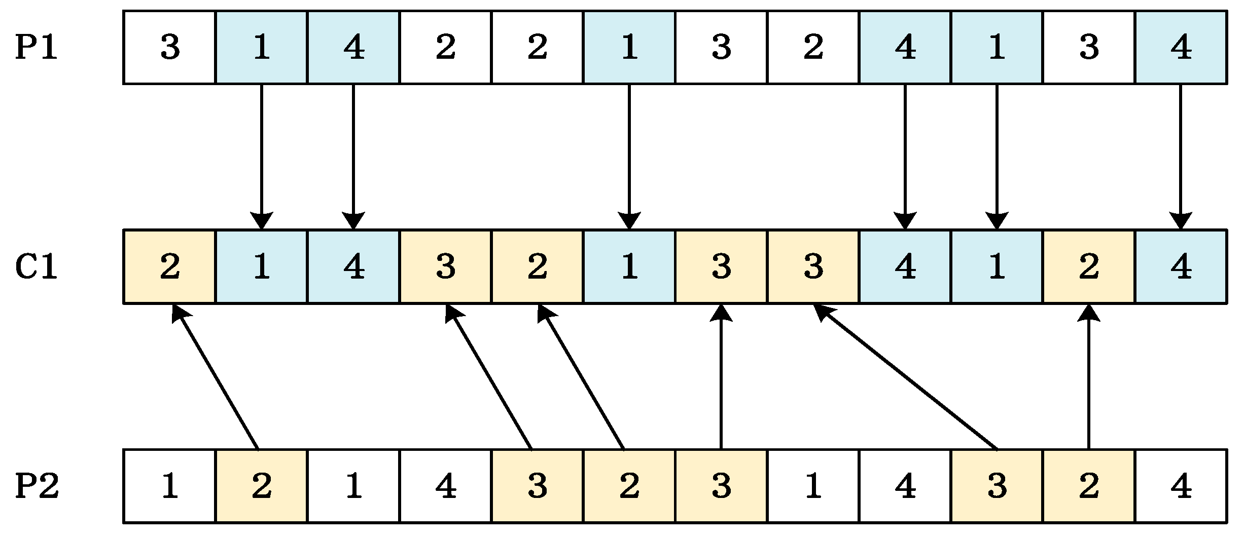
The crossover operation is considered as the backbone of GA, and its purpose is to inherit the characteristics of the parental solutions to generate two offspring solutions. In order to reduce the computational cost, it is always hoped that the offspring solutions produced after the crossover are feasible solutions. Based on the above two considerations, this study uses the POX operator to perform the crossover operation. The specific operation steps of POX operator are as follows.
- Step 1:
- All jobs are randomly separated into two non-empty subsets, denoted as JS1 and JS2. The initial population is produced in cell 1, and the initial population size is N. Initially, cell 2 and cell 3 are both empty;
- Step 2:
- Copy the job numbers contained in the job subset JS1 (JS2) in the parent chromosome P1 (P2) directly to the child C1 (C2), and keep their position and order;
- Step 3:
- Copy the job numbers contained in the job subset JS2 (JS1) in the parent chromosome P2 (P1) to the child C1 (C2), just keep their order unchanged.
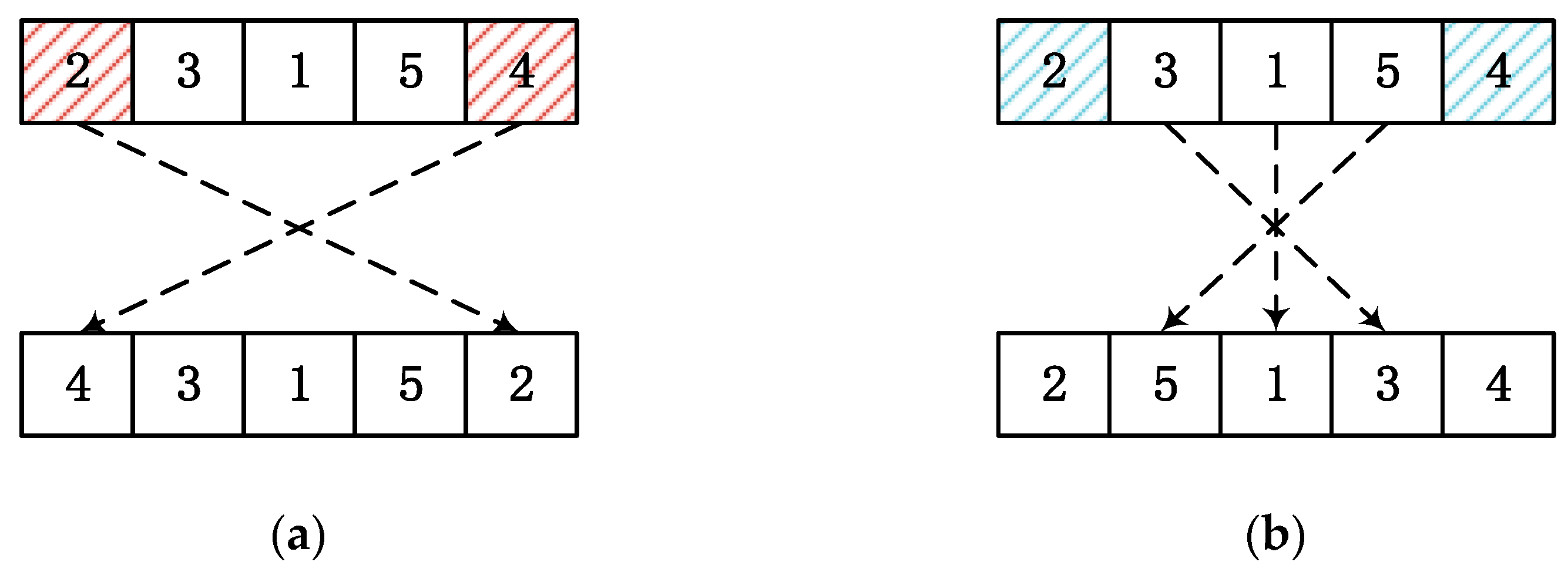
Take the chromosome encoding with 4 jobs as an example, suppose JS1 = {1, 4}, JS2 = {2, 3}, then the newly generated child C1 after crossover is shown in Figure 4. In the same way, after a crossover operation, a child C2 will also be generated.
The purpose of mutation operation is to bring slight disturbance to the population, which can enhance the diversity of the population. The mutation operator in this work is implemented by randomly selecting one of the two mutation operators with equal probability. They are swap mutation and inversion mutation as shown in Figure 5.
In classic GA, the crossover probability and mutation probability remain unchanged throughout the evolution process, but actual research shows that they are the key to GA performance [32]. The crossover and mutation probability of conventional adaptive GA is expressed as follows:
Among them, Pc and Pm are the adaptive crossover and mutation probabilities, α1, α2, α3, α4 are constants. Fc is the larger fitness value of the two individuals to be crossed. Fm is the fitness value of the current mutant individual. Fmax is the maximum fitness value in the population. Favg is the average fitness value of the population.
The value of the crossover probability determines the update rate of the population. If its value is too large, it will destroy the excellent genetic model. If the value is too small, it will reduce the search efficiency of the algorithm and it is difficult to effectively improve the population. Therefore, this work combines two considerations to improve the conventional adaptive probability. On the one hand, in the early stage of evolution, in order to expand the overall search range and speed up the population update rate, should be increased; In the later stage of evolution, the overall solution set of the population tends to be stable. In order to keep the good genes better, should be appropriately reduced. On the other hand, considering the destructiveness of the crossover operator to the chromosome structure, individuals with poor fitness are given a higher value. Conversely, for individuals with higher fitness values, in order to reduce the damage to excellent genes, the value should be appropriately reduced. The case of mutation probability is similar. Considering the above two aspects, the improved adjustment mechanism is set as follows.
Among them, Pc1 (Pm1) represents the maximum crossover (mutation) probability, which is related to the number of iterations of evolution. Pc2 = 0.6 (Pm2 = 0.1) is the minimum crossover (mutation) probability. IT denotes the maximum number of iterations of the evolution process. t means the current number of iterations. The factor 2 in the denominator in square brackets is to ensure that the maximum value of this part does not exceed the integer 1.
3.3. Evolutionary Rule of Objects in Cell 2
The evolution rule in cell 2 is a discretized improvement of rumor PSO, which is a variant of traditional PSO algorithm. The traditional PSO was proposed by Kennedy [33,34] through observing the social behavior of birds and other biological groups. It is a simple model constructed by swarm intelligence. The initial solution is generated by the random given velocity, while the new solution depends on the competition and cooperation among particle swarm. The best position of the particle itself and the best position of the entire population are two key factors for seeking the optimal solution or the approximate optimal solution. This is similar to human behavior in decision-making: people focus not only on their own best experiences, but also on the best experiences of others around them. The standard PSO equations [35] that can reflect the nature of the above-mentioned swarm intelligence evolution is as follows. Due to its excellent characteristics such as fast convergence and high feasibility, PSO has been applied in many fields.
where Vi(t) and Xi(t) respectively represent the velocity and position of the i-th particle (chromosome) in the t-th iteration; Pib denotes the historical best position of the i-th particle; Pgb stands for the best position in the history of all particles; w is the inertia weight; c1 and c2 are learning factors; r1, r2 are two independent random numbers uniformly distributed between (0,1).
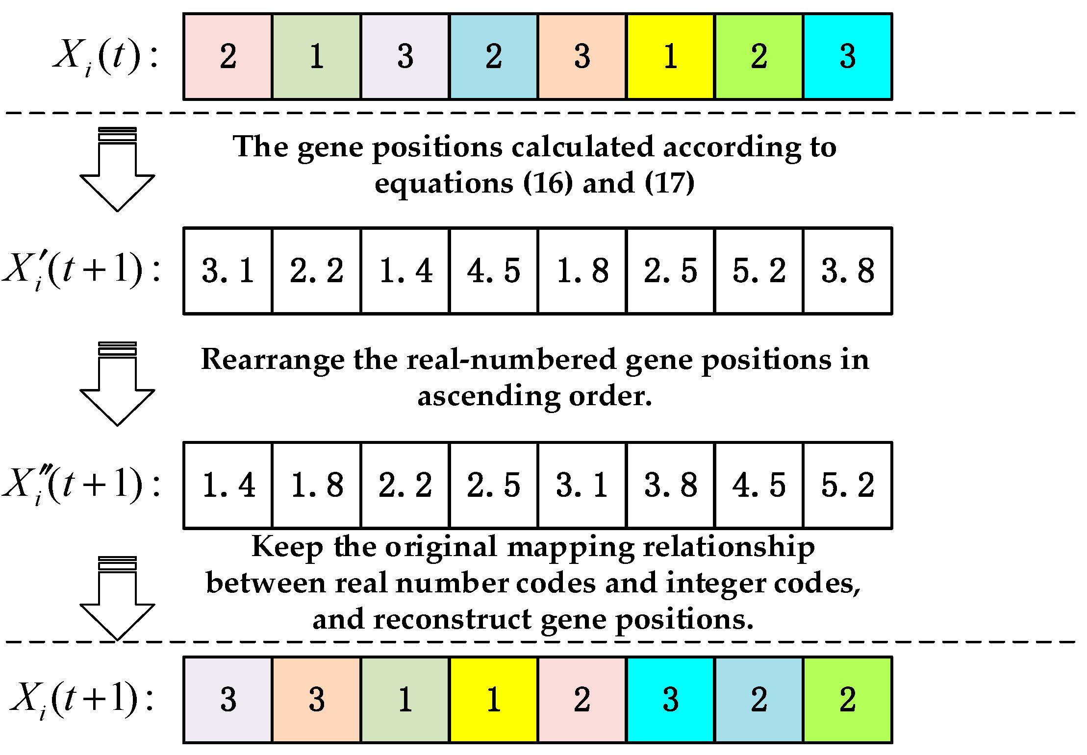
The rumor PSO proposed by Clerc has shown excellent performance in dealing with continuous problems [31]. In order to avoid the population falling into the local optimum and improve the diversity of the population as much as possible, the difference from the traditional PSO is that rumor PSO does not use the global optimum position information (Pgb) to guide the entire population. The equation of rumor PSO is shown in (16) (17).
Among them, PKb replaces Pgb in the standard PSO, which represents the best historical position among K particles randomly selected from the entire population. In this paper, K = 3 is set according to Clerc’s research results [31]. As the iteration progresses, the object information is exchanged and spread from K particles to the entire population. This communication mechanism allows the particle trajectory to appear circuitous, and its propagation process is similar to the spread of rumors, so it is called rumor PSO.
By introducing a real-coded ascending mapping method, rumor PSO can be effectively applied to the JSSP which belongs to the discrete combinatorial optimization problem. The specific evolution process is carried out according to the following steps, and Figure 6 shows an evolutionary process taking the partial encoding of a chromosome as an example.
- Step 1:
- Receive the initialized population, the population size is N;
- Step 2:
- Determine whether the iteration threshold is reached. If yes, stop and use the historical optimal value of N particles as the output result. If not, go to Step 3;
- Step 3:
- For each particle, that is, the chromosome, K particles are randomly selected from the population. Evaluate the historical optimal fitness value of these K particles to determine PKb, and then use Equations (16) and (17) to update each particle;
- Step 4:
- Rearrange the real-numbered gene positions in ascending order;
- Step 5:
- Keep the original mapping relationship between real number codes and integer codes, and reconstruct gene positions;
- Step 6:
- Evaluate the newly generated particle, and if its fitness value is better, replace the Pib value corresponding to this particle. Continue to Step 2.
3.4. Evolutionary Rule of Objects in Cell 3
The evolutionary rules in cell 3 are guided by a local search method (LSM). The LSM proposed in this work consists of two parts, namely, an algorithm for quickly identifying critical path, and a neighborhood optimization algorithm based on critical path.
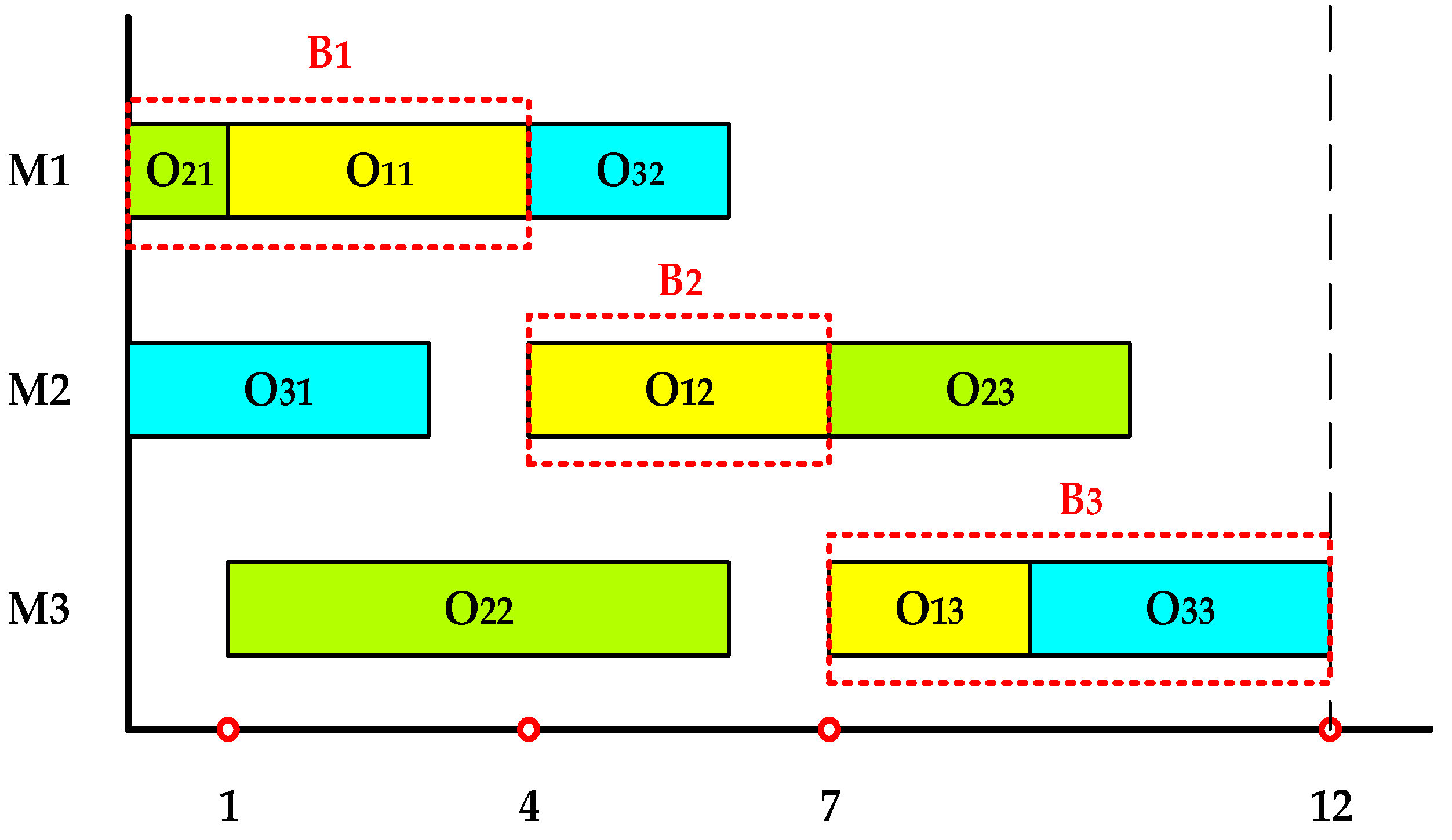
An important part of the feasible solution of JSSP is the critical path, which is the longest path from the starting point (0) to the ending point (1) in the disjunction graph. The length of the critical path is also called the makespan of a scheduling solution. The set of operations based on the critical path is recognized as a critical operation. The critical path can be broken down into several blocks (B1, B2, …, Br). Each block refers to the longest sequence of adjacent critical operations processed on the same machine. It should be noted that for every two consecutive blocks Bj and Bj+1, the last operation of Bj and the first operation of Bj+1 should belong to the same job but be processed on different machines. Considering that the permutation of non-critical adjacent operations does not help to improve the makespan of the scheduling solution and may even lead to infeasible solutions. Therefore, the LSM in this work will only implement the exploration and exploitation of individual neighborhoods based on the critical path.
In order to perform an effective neighborhood search based on the critical path, an algorithm for quickly finding and identifying the critical path of a feasible solution is first proposed. The notations S(Oij) and E(Oij) represent the start time and end time of the operation Oij, respectively. The specific algorithm steps to identify the critical path are as follows.
- Step 1:
- Let , . The set Q is used to store the operations in the critical path, and it is initially an empty set;
- Step 2:
- Check each element τ in the set P. If for , the expression E(τ) = S(λ) is not satisfied, then operation τ is deleted from the set P;
- Step 3:
- Choose an operation σ that satisfies S(σ) = 0 from the updated set P, and add it to Q. Let w = 1;
- Step 4:
- While (E(σw) ≠ makespan) then w = w + 1, choose an operation satisfied S(σw) = E(σw−1) and add σw to Q.
- Step 5:
- Output the elements in Q in order, which is the required critical path.
Take another instance of 3 × 3 JSSP presented in Table 2 as an example to illustrate the concepts of critical path and blocks. Assuming that an approximate optimal solution of this instance is 2-3-1-2-1-3-1-2-3, the Gantt chart corresponding to the feasible solution is shown in Figure 7 and the makespan of this solution is 12. According to the above algorithm to identify the critical path of this feasible solution, the set Q = {O21, O11, O12, O13, O33} can be easily obtained. In other words, the critical path is O21 → O11 → O12 → O13 → O33. This critical path can be broken down into three blocks B1, B2, and B3.
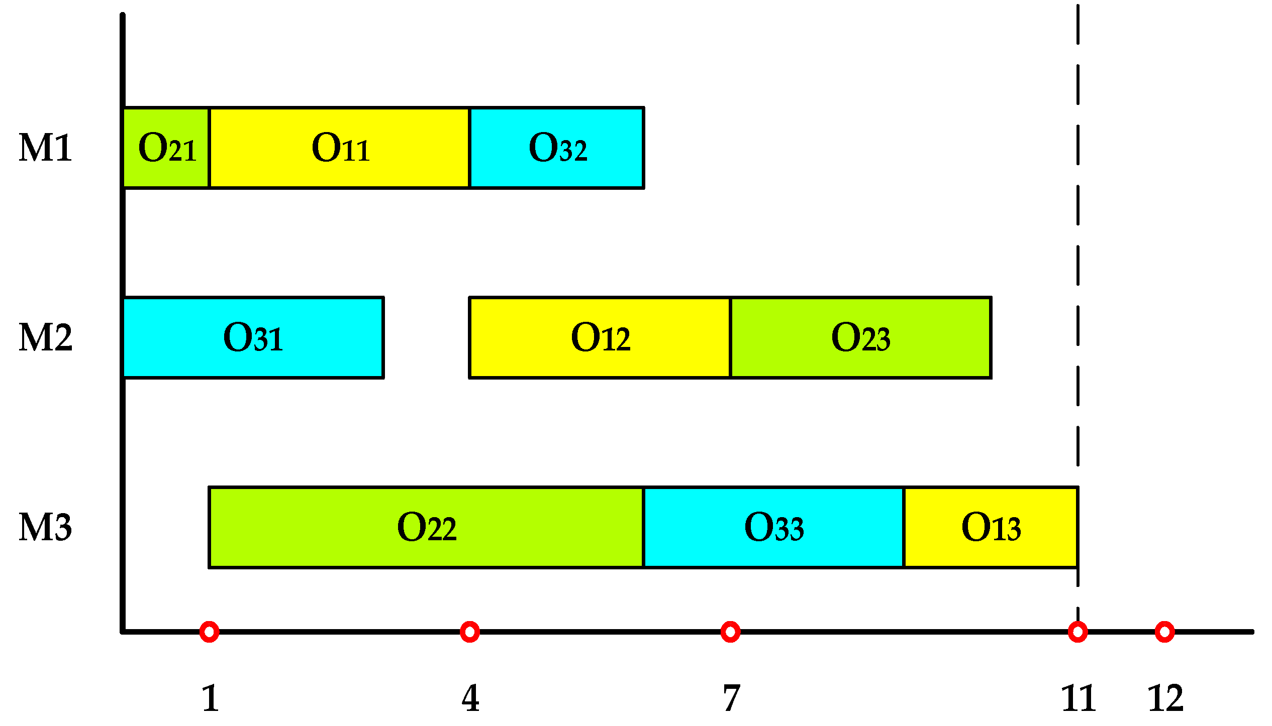
With an algorithm for quickly identifying the critical path, it is possible to implement further neighborhood optimization for the already better individuals. The steps of the specific neighborhood search algorithm are as follows.
- Step 1:
- Receive N feasible solutions optimized by GA and PSO (also can be regarded as approximate optimal solutions);
- Step 2:
- For each approximate optimal solution, use the algorithm given above to identify the critical path and its blocks;
- Step 3:
- According to the start and end time of the block, determine whether the current block is the first block or the last block. If it is the first block, exchange the last two operations; if it is the tail block, exchange the first two blocks. For the internal blocks, the first two operations and the last two operations of the block are exchanged respectively. All the operations after the exchange are allocated to the corresponding machines in the best available processing time. If only one operation is contained in a block, no exchange is performed;
- Step 4:
- As long as the makespan is improved, the current exchange is accepted. Otherwise, the current exchange is cancelled;
- Step 5:
- If an exchange is accepted, the original critical path may be destroyed. Go to Step 2, re-identify its critical path and perform a neighborhood search;
- Step 6:
- If the exchange in any block of the critical path does not improve the optimal goal, stop the local search.
3.5. Flow Chart of the Proposed Hybrid Algorithm
This section presents a flow chart integrating different heuristic algorithms, as shown in Figure 9. The three main sub-algorithms are: improved adaptive GA, discretized rumor PSO, and improved LSM that can quickly identify critical path. As mentioned earlier, the above three sub-algorithms correspond to the evolution rules in the three cells in the tissue-like membrane system.
4. Comparative Experiment and Discussion
The algorithm proposed in this work is implemented by Python. The computer used for computation has an i5-4210H processor with a 2.90 GHz clock speed and 12 GB of RAM. The parameter settings involved in the algorithm are as follows. The initial population size is N = 128. The maximum number of external iterations used to control the population update is Iex = 20. The maximum number of iterations of modified PSO and improved GA, that is, the number of internal iterations in cell 1 and cell 2 are both Iin = 50. The inertia weight in Equation (16) is w = 0.7, and the learning factor c1 = c2 = 2.10.
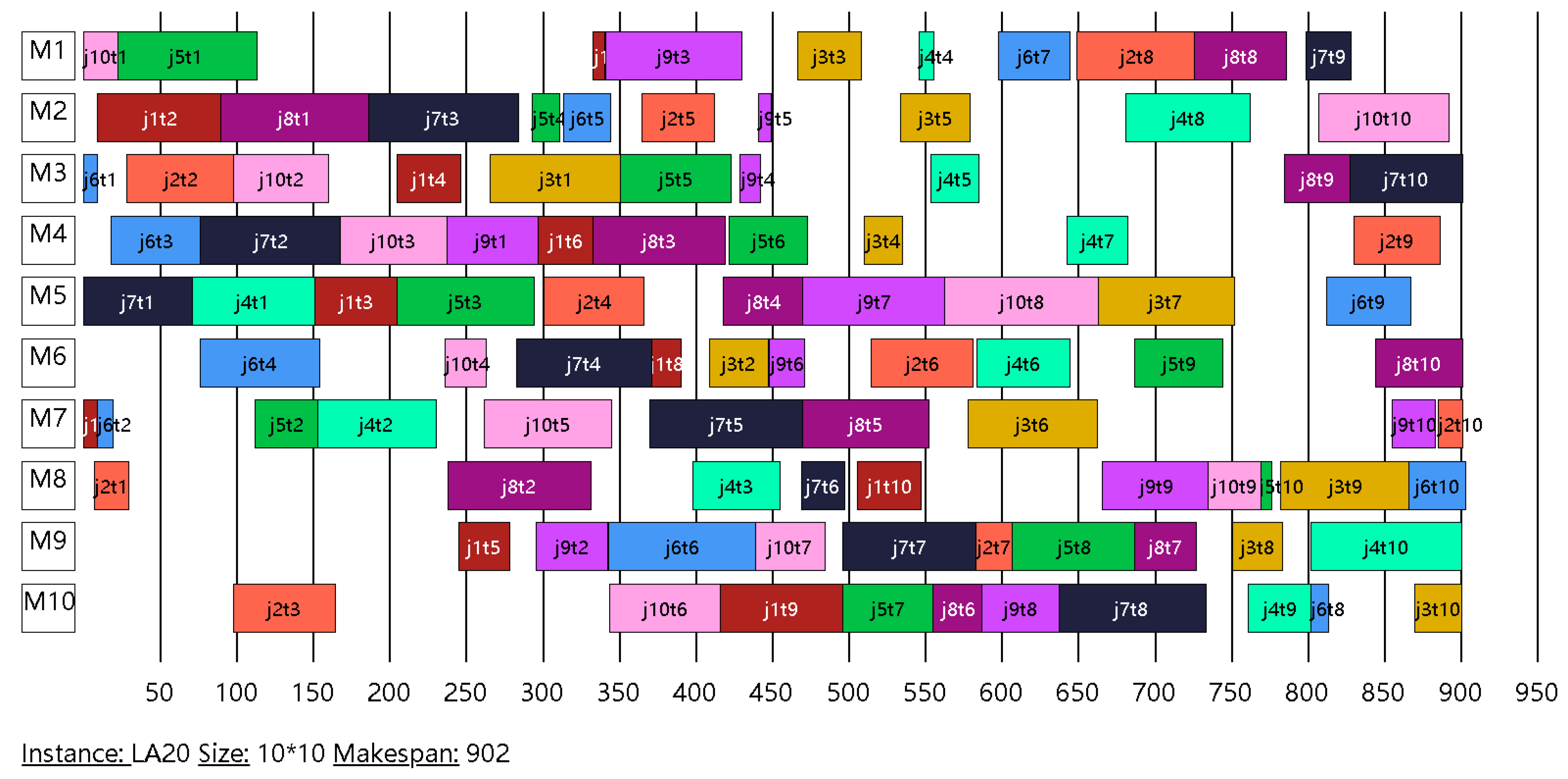
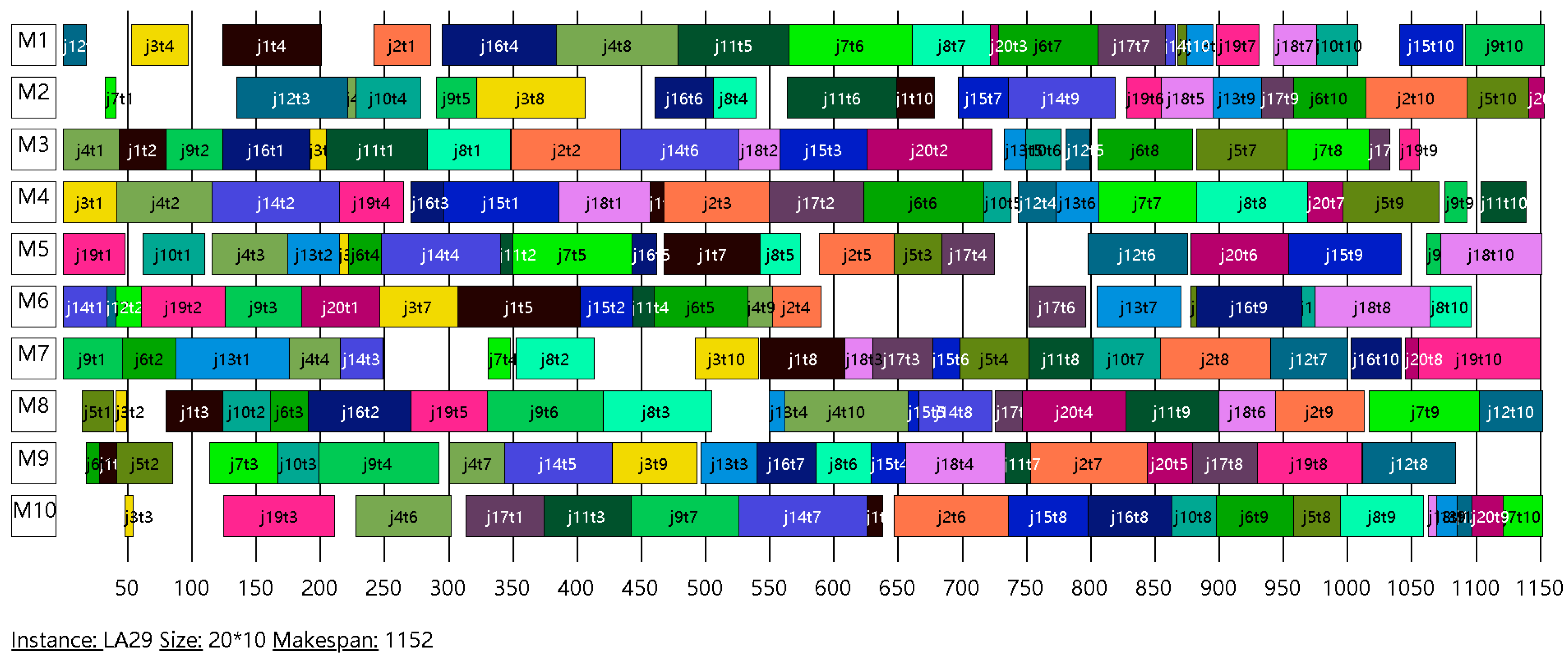
The proposed algorithm is first compared with three state-of-the-art heuristic algorithms on 22 JSSP benchmark instances (see Table 3). Among them, there are 1 instance (FT20) designed by Fisher and Thompson [2], and 21 instances (LA01~LA40) designed by Lawrence [36]. The other three heuristic algorithms used for comparison are MAGATS [19], NIMGA [37], and HIMGA [8]. In Table 3, the first column is the instance name, the second column is the instance size n × m, and the third column is the best-known solution (BKS). The remaining four columns are the best solutions obtained by different algorithms on corresponding instances. The results show that, except for the instances LA36 and LA40, the BKS of the remaining instances can be found by the proposed algorithm. Figure 10 and Figure 11 show the Gantt chart of the experimental results of the instances LA20 and LA29, respectively, while the remaining algorithms for comparison did not get BKS on these two instances. The results of the comparison algorithms come from the corresponding original publication [8,19].
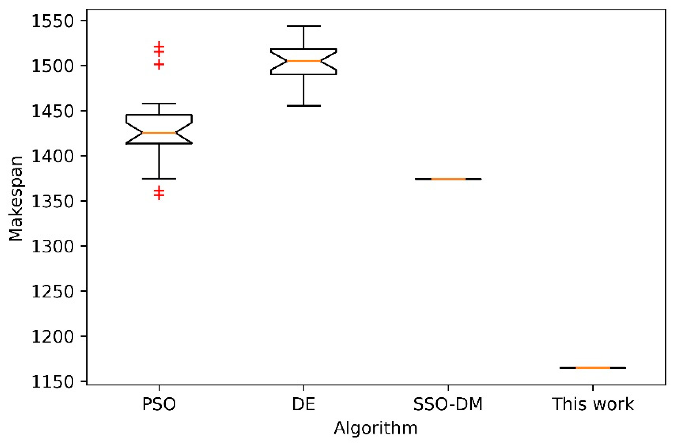
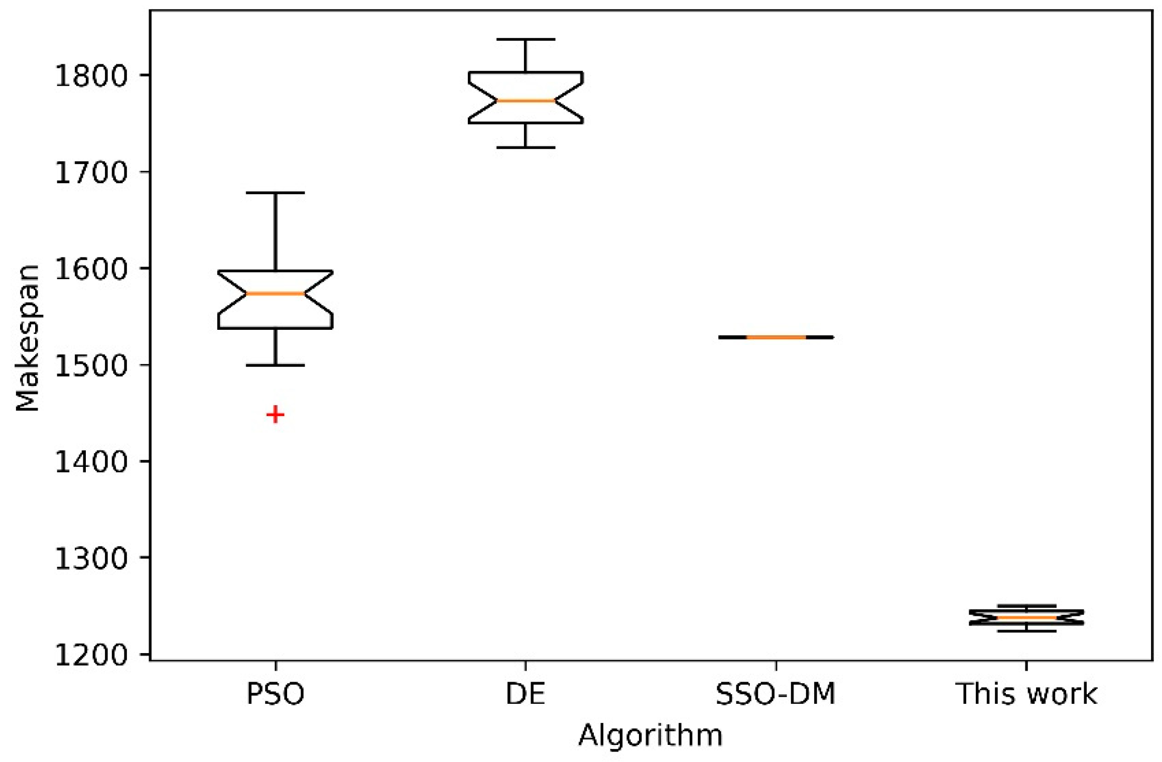
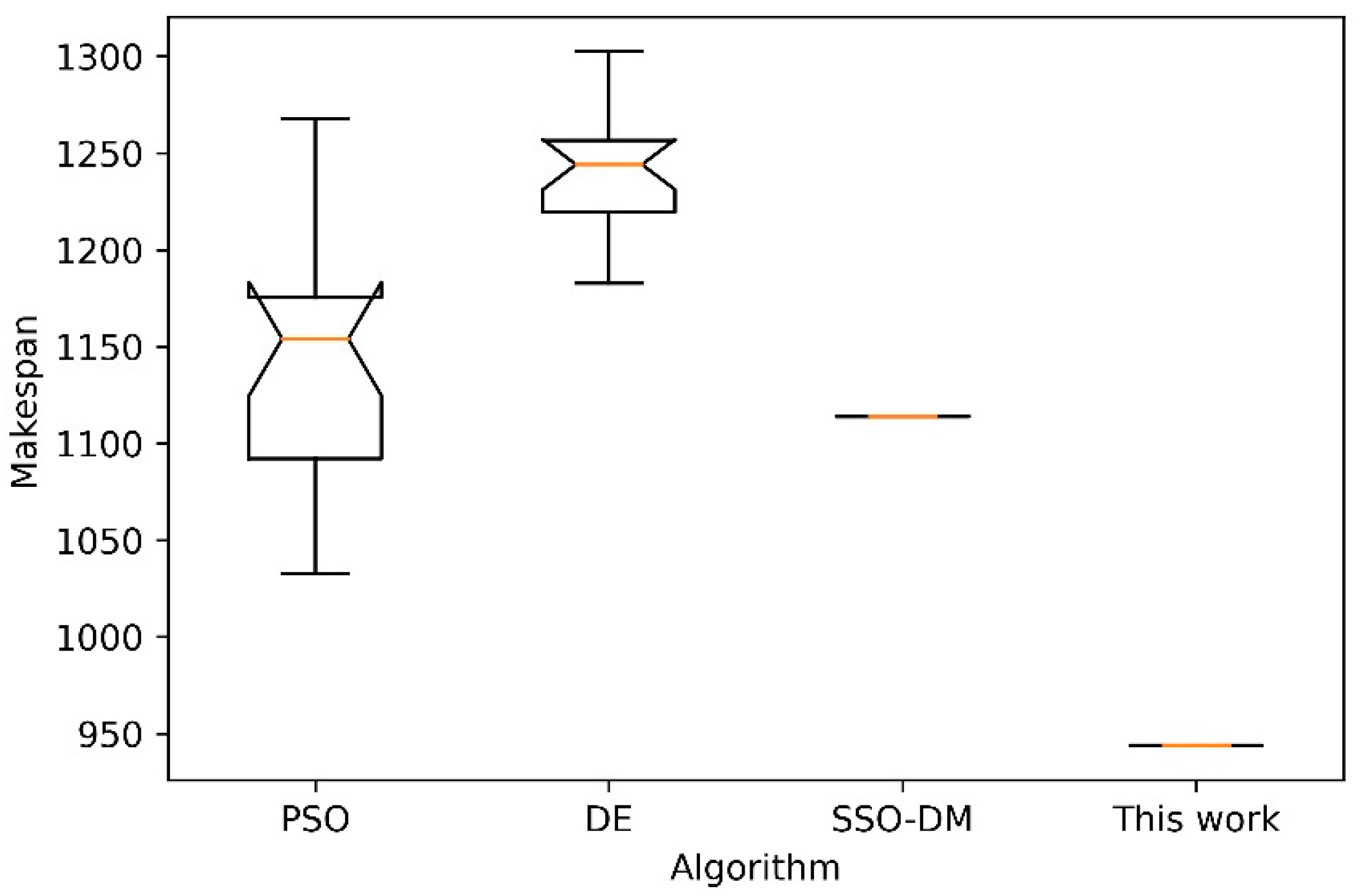
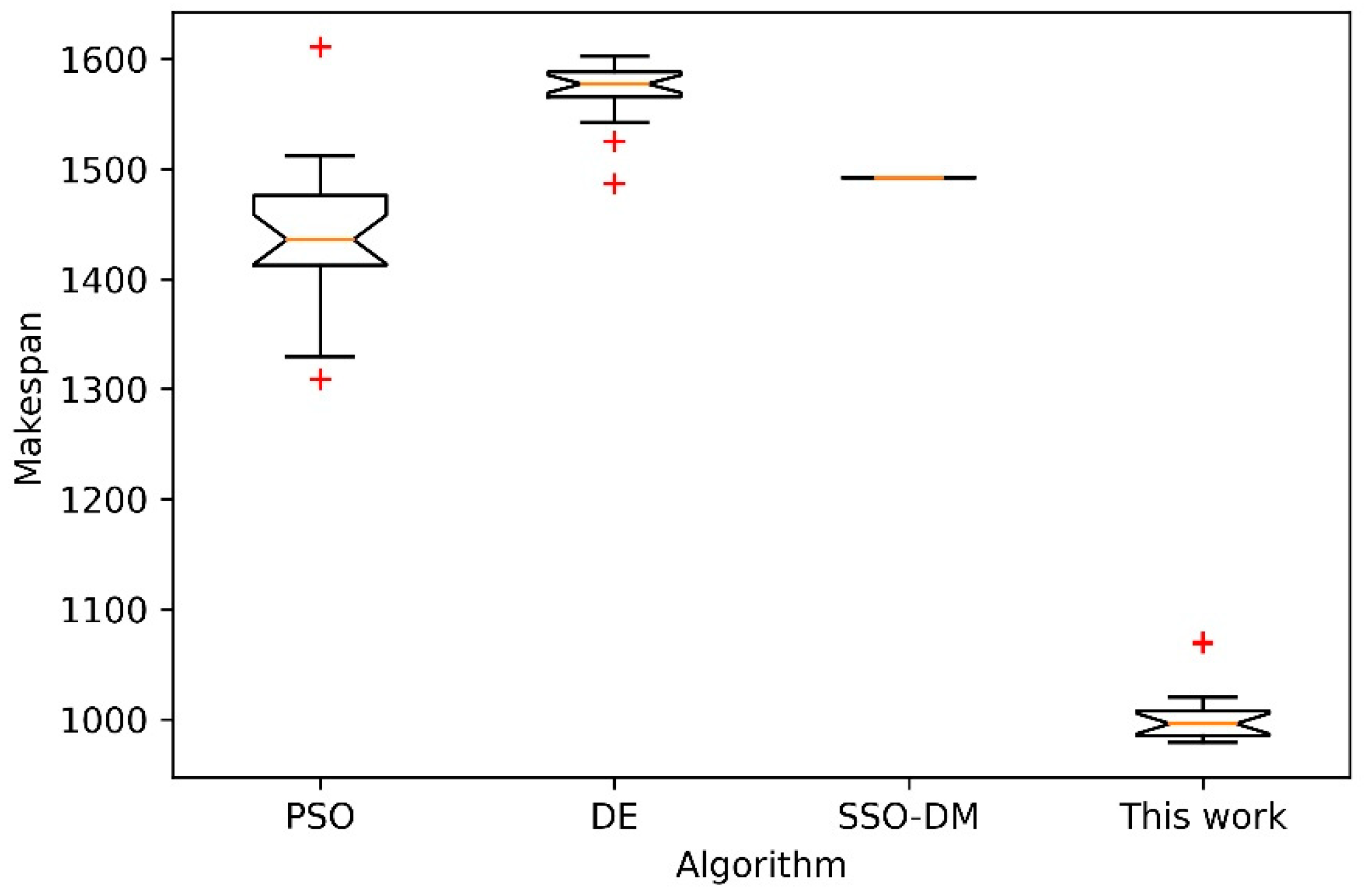
Next, further comparative analysis is done on four instances of different sizes with the other 3 heuristic algorithms. The three comparison algorithms are PSO [11], DE [38] and SSO-DM [18]. Four instances of different sizes are FT10, LA40, ORB10 [39] and YN4 [40]. For 20 independent runs of each algorithm, Table 4 shows the statistical results of the best, worst, mean and standard deviation (Std.). The comparison data of the above three algorithms in Table 4 are from the literature [18]. Figure 12, Figure 13, Figure 14 and Figure 15 show the box plots of these four algorithms on the four instances. Box plot is a popular visual representation of data distribution. The horizontal line in the box is used to indicate the median. The red plus sign in the figure indicates possible outliers. Although the stability of the proposed algorithm is slightly inferior to SSO-DM, the accuracy of its solution is better than the other three algorithms. Figure 16 shows a Gantt chart of an optimal solution for the instance ORB10.
5. Conclusions
This work introduces the inherent mechanism of tissue-like P system for solving the job shop scheduling problem and proposes a hybrid heuristic algorithm based on this framework. The algorithm framework incorporates improved genetic algorithms (GA), modified rumor particle swarm optimization (PSO), and a local search method based on rapid identification of critical path. Through comparative experiments in multiple benchmark instances of JSSP, comprehensively, the proposed algorithm performs better than the other comparison algorithms.
However, although this work couples the traditional hybrid heuristic algorithm with the tissue-like membrane system, it still has some shortcomings. That is, this coupling is only a formal simulation, and does not truly reflect the advantages of the distribution and parallelism of membrane computing. With the continuous development of hardware technology, the realization of parallel computing will better simulate the parallel advantages of membrane computing. This will also greatly reduce the optimization time of the algorithm. In addition, this work is dedicated to solving single-objective JSSP, and in actual industrial production, the demand for multi-objective optimization is increasing day by day.
Based on this, there will be several meaningful research directions in the future. First of all, in order to make full use of and simulate the parallelism of membrane computing, it is still a promising and challenging direction to develop multi-threaded parallel computing algorithms and implement them on GPUs. Secondly, the multi-objective flexible job shop scheduling problem, as the top problem of the shop scheduling problem, will become an important research direction that we continue to carry out based on the current work. In addition, as the two most important branches of biological computing, the combination of membrane computing and DNA computing will also become an extremely interesting and valuable cross field.
Author Contributions
Conceptualization, X.T. and X.L.; methodology, X.T. and X.L.; software, X.T.; validation, X.T.; formal analysis, X.T.; writing—original draft preparation, X.T.; writing—review and editing, X.T. and X.L.; supervision, X.L.; project administration, X.L.; funding acquisition, X.L. All authors have read and agreed to the published version of the manuscript.
Funding
This work was partly supported by the National Natural Science Foundation of China (Nos. 61876101, 61802234, 61806114), the Social Science Fund Project of Shandong (Nos. 11CGLJ22, 16BGLJ06), the Natural Science Foundation of the Shandong Province (No. ZR2019QF007), the Youth Fund for Humanities and Social Sciences, Ministry of Education (No. 19YJCZH244), the China Postdoctoral Special Funding Project (No. 2019T120607), and the China Postdoctoral Science Foundation Funded Project (Nos. 2017M612339, 2018M642695).
Data Availability Statement
This study did not report any data. All test instances and comparison data can be publicly accessed and freely obtained from the corresponding references. We have made a detailed description and quotation in the text.
Conflicts of Interest
The authors declare no conflict of interest.
References
- Giffler, B.; Thompson, G.L. Algorithms for solving production-scheduling problems. Oper. Res. 1960, 8, 487–503. [Google Scholar] [CrossRef]
- Fisher, H.; Thompson, G.L. Probabilistic learning combinations of local job-shop scheduling rules. Ind. Sched. 1963, 225–251. [Google Scholar]
- Balas, E. Machine sequencing via disjunctive graphs: An implicit enumeration algorithm. Oper. Res. 1969, 17, 941–957. [Google Scholar] [CrossRef]
- Lageweg, B.J.; Lenstra, J.K.; Rinnooy Kan, A.H.G. Job-shop scheduling by implicit enumeration. Manag. Sci. 1977, 24, 441–450. [Google Scholar] [CrossRef]
- Carlier, J.; Pinson, E. An algorithm for solving the job-shop problem. Manag. Sci. 1989, 35, 164–176. [Google Scholar] [CrossRef]
- Blackstone, J.H.; Phillips, D.T.; Hogg, G.L. A state-of-the-art survey of dispatching rules for manufacturing job shop operations. Int. J. Prod. Res. 2007, 20, 27–45. [Google Scholar] [CrossRef]
- Adams, J.; Balas, E.; Zawack, D. The shifting bottleneck procedure for job shop scheduling. Manag. Sci. 1988, 34, 391–401. [Google Scholar] [CrossRef]
- Kurdi, M. A new hybrid island model genetic algorithm for job shop scheduling problem. Comput. Ind. Eng. 2015, 88, 273–283. [Google Scholar] [CrossRef]
- Watanabe, M.; Ida, K.; Gen, M. A genetic algorithm with modified crossover operator and search area adaptation for the job-shop scheduling problem. Comput. Ind. Eng. 2005, 48, 743–752. [Google Scholar] [CrossRef]
- Lian, Z.; Jiao, B.; Gu, X. A similar particle swarm optimization algorithm for job-shop scheduling to minimize makespan. Appl. Math. Comput. 2006, 183, 1008–1017. [Google Scholar] [CrossRef]
- Lin, T.-L.; Horng, S.-J.; Kao, T.-W.; Chen, Y.-H.; Run, R.-S.; Chen, R.-J.; Lai, J.-L.; Kuo, I.H. An efficient job-shop scheduling algorithm based on particle swarm optimization. Expert. Syst. Appl. 2010, 37, 2629–2636. [Google Scholar] [CrossRef]
- Fığlalı, N.; Özkale, C.; Engin, O.; Fığlalı, A. Investigation of ant system parameter interactions by using design of experiments for job-shop scheduling problems. Comput. Ind. Eng. 2009, 56, 538–559. [Google Scholar] [CrossRef]
- Satake, T.; Morikawa, K.; Takahashi, K.; Nakamura, N. Simulated annealing approach for minimizing the makespan of the general job-shop. Int. J. Prod. Econ. 1999, 60–61, 515–522. [Google Scholar] [CrossRef]
- Zhang, C.Y.; Li, P.G.; Guan, Z.L.; Rao, Y.Q. A tabu search algorithm with a new neighborhood structure for the job shop scheduling problem. Comput. Oper. Res. 2007, 34, 3229–3242. [Google Scholar] [CrossRef]
- Zhang, C.Y.; Li, P.G.; Rao, Y.Q.; Li, S.Z. A new hybrid GA/SA algorithm for the job shop scheduling problem. Lect. Notes Comput. Sc. 2005, 3448, 246–259. [Google Scholar]
- Zhang, C.Y.; Rao, Y.Q.; Li, P.G. An effective hybrid genetic algorithm for the job shop scheduling problem. Int. J. Adv. Manuf. Technol. 2008, 39, 965–974. [Google Scholar] [CrossRef]
- Abdel-Kader, R.F. An improved PSO algorithm with genetic and neighborhood-based diversity operators for the job shop scheduling problem. Appl. Artif. Intell. 2018, 32, 433–462. [Google Scholar] [CrossRef]
- Zhou, G.; Zhou, Y.; Zhao, R. Hybrid social spider optimization algorithm with differential mutation operator for the job-shop scheduling problem. J. Ind. Manag. Optim. 2019, 13, 1–16. [Google Scholar] [CrossRef] [Green Version]
- Peng, C.; Wu, G.; Liao, T.W.; Wang, H. Research on multi-agent genetic algorithm based on tabu search for the job shop scheduling problem. PLoS ONE 2019, 14, e0223182. [Google Scholar] [CrossRef]
- Pongchairerks, P. A two-level metaheuristic algorithm for the job-shop scheduling problem. Complexity 2019, 2019, 1–11. [Google Scholar] [CrossRef]
- Cruz-Chavez, M.A.; Rosales, M.H.C.; Zavala-Diaz, J.C.; Aguilar, J.A.H.; Rodriguez-Leon, A.; Avelino, J.C.P.; Ortiz, M.E.L.; Salinas, O.H. Hybrid micro genetic multi-population algorithm with collective communication for the job shop scheduling problem. IEEE Access 2019, 7, 82358–82376. [Google Scholar] [CrossRef]
- Păun, G. Computing with membranes. J. Comput. Syst. Sci. 2000, 61, 108–143. [Google Scholar] [CrossRef] [Green Version]
- Martin-Vide, C.; Păun, G.; Pazos, J.; Rodriguez-Paton, A. Tissue P systems. Theor. Comput. Sci. 2003, 296, 295–326. [Google Scholar] [CrossRef] [Green Version]
- Bernardini, F.; Gheorghe, M. Cell communication in tissue P systems: Universality results. Soft Comput. 2005, 9, 640–649. [Google Scholar] [CrossRef]
- Păun, A.; Păun, G. Small universal spiking neural P systems. Biosystems 2007, 90, 48–60. [Google Scholar] [CrossRef] [PubMed] [Green Version]
- Wang, J.; Shi, P.; Peng, H.; Perez-Jimenez, M.J.; Wang, T. Weighted fuzzy spiking neural P systems. IEEE Trans. Fuzzy Syst. 2013, 21, 209–220. [Google Scholar] [CrossRef]
- Song, B.S.; Zhang, C.; Pan, L.Q. Tissue-like P systems with evolutional symport/antiport rules. Inform. Sci. 2017, 378, 177–193. [Google Scholar] [CrossRef]
- Peng, H.; Shi, P.; Wang, J.; Riscos-Núñez, A.; Pérez-Jiménez, M.J. Multiobjective fuzzy clustering approach based on tissue-like membrane systems. Knowl. Based Syst. 2017, 125, 74–82. [Google Scholar] [CrossRef]
- Jiang, Z.; Liu, X. A novel consensus fuzzy k-modes clustering using coupling DNA-chain-hypergraph P system for categorical data. Processes 2020, 8, 1326. [Google Scholar] [CrossRef]
- Guo, W.; Liu, X.; Xiang, L. Membrane system-based improved neural networks for time-series anomaly detection. Processes 2020, 8, 1168. [Google Scholar] [CrossRef]
- Clerc, M. Particle Swarm Optimization; John Wiley & Sons: Hoboken, NJ, USA, 2010; Volume 93. [Google Scholar]
- Srinivas, M.; Patnaik, L.M. Adaptive probabilities of crossover and mutation in genetic algorithms. IEEE Trans. Syst. Man Cybern. 1994, 24, 656–667. [Google Scholar] [CrossRef] [Green Version]
- Kennedy, J.; Eberhart, R. Particle swarm optimization. In Proceedings of the IEEE International Conference on Neural Networks Proceedings, Perth, WA, Aaustralia, 27 November–1 December 1995; pp. 1942–1948. [Google Scholar]
- Kennedy, J. Particle swarm optimization. Encycl. Mach. Learn. 2010, 4, 760–766. [Google Scholar]
- Bratton, D.; Kennedy, J. Defining a standard for particle swarm optimization. In Proceedings of the 2007 IEEE Swarm Intelligence Symposium (SIS 2007), Honolulu, HI, USA, 1–5 April 2007; pp. 120–127. [Google Scholar]
- Lawrence, S. Supplement to resource constrained project scheduling: An experimental investigation of heuristic scheduling techniques. Grad. Sch. Ind. Adm. 1984, 4, 4411–4417. [Google Scholar]
- Kurdi, M. An effective new island model genetic algorithm for job shop scheduling problem. Comput. Oper. Res. 2016, 67, 132–142. [Google Scholar] [CrossRef]
- Zobolas, G.I.; Tarantilis, C.D.; Ioannou, G. A hybrid evolutionary algorithm for the job shop scheduling problem. J. Oper. Res. Soc. 2009, 60, 221–235. [Google Scholar] [CrossRef]
- Applegate, D.; Cook, W. A computational study of the job-shop scheduling problem. ORSA J. Comput. 1991, 3, 85–176. [Google Scholar] [CrossRef]
- Yamada, T.; Nakano, R. A genetic algorithm applicable to large-scale job-shop problems. Parallel Probl. Solving Nat. 1992, 2, 281–290. [Google Scholar]
Figure 1.
The disjunctive graph representation of a 3 × 3 JSSP (job shop scheduling problem).

Figure 2.
The structure of the coupled membrane system.

Figure 3.
Gantt chart for the encoding sequence 1-3-2-2-1-3-3-1-2.

Figure 4.
Demonstration of POX (precedence operation crossover) operator.

Figure 5.
Two mutation operators that can be selected with equal probability. (a) Swap mutation; (b) Inversion mutation.
Figure 5.
Two mutation operators that can be selected with equal probability. (a) Swap mutation; (b) Inversion mutation.

Figure 6.
Demonstration of the update process of the discretized rumor PSO (particle swarm optimization).
Figure 6.
Demonstration of the update process of the discretized rumor PSO (particle swarm optimization).

Figure 7.
The critical path corresponding to the approximate optimal solution and its three blocks.

Figure 8.
The Gantt chart corresponding to the optimal solution obtained after local search.

Figure 9.
The overall flow chart of the algorithm framework.

Figure 10.
Gantt chart of an optimal schedule of instance LA20 (designed by Lawrence).

Figure 11.
Gantt chart of an optimal schedule of instance LA29 (designed by Lawrence).

Figure 12.
The box plot for FT20 (designed by Fisher & Thompson).

Figure 13.
The box plot for LA40 (designed by Lawrence).

Figure 14.
The box plot for ORB10 (designed by Applegate & Cook).

Figure 15.
The box plot for YN4 (designed by Yamada & Nakano).

Figure 16.
Gantt chart of an optimal schedule of instance ORB10 (designed by Applegate & Cook).


Table 1.
A 3 × 3 JSSP (job shop scheduling problem).
| Operation | J1 | J2 | J3 | |||
|---|---|---|---|---|---|---|
| Machine | Machine | Machine | ||||
| 1 | 3 | 7 | 2 | 5 | 2 | 4 |
| 2 | 1 | 4 | 3 | 6 | 1 | 2 |
| 3 | 2 | 2 | 1 | 3 | 3 | 3 |
Table 2.
An instance of 3 × 3 JSSP.
| Operation | J1 | J2 | J3 | |||
|---|---|---|---|---|---|---|
| Machine | Machine | Machine | ||||
| 1 | 1 | 3 | 1 | 1 | 2 | 3 |
| 2 | 2 | 3 | 3 | 5 | 1 | 2 |
| 3 | 3 | 2 | 2 | 3 | 3 | 3 |
Table 3.
Comparison of the best solutions with other works.
| Instances | Size | BKS | This Work | MAGATS | NIMGA | HIMGA |
|---|---|---|---|---|---|---|
| FT20 | 20 × 5 | 1165 | 1165 | 1165 | 1173 | 1165 |
| LA05 | 10 × 5 | 593 | 593 | 593 | 593 | 593 |
| LA10 | 15 × 5 | 958 | 958 | 958 | 958 | 958 |
| LA15 | 20 × 5 | 1207 | 1207 | 1207 | 1207 | 1207 |
| LA20 | 10 × 10 | 902 | 902 | 907 | 907 | 902 |
| LA21 | 15 × 10 | 1046 | 1046 | 1046 | 1058 | 1046 |
| LA22 | 15 × 10 | 927 | 927 | 927 | 937 | 927 |
| LA23 | 15 × 10 | 1032 | 1032 | 1032 | 1032 | 1032 |
| LA24 | 15 × 10 | 935 | 935 | 935 | 947 | 935 |
| LA25 | 15 × 10 | 977 | 977 | 977 | 989 | 977 |
| LA26 | 20 × 10 | 1218 | 1218 | 1218 | 1218 | 1218 |
| LA27 | 20 × 10 | 1235 | 1235 | 1235 | 1269 | 1235 |
| LA28 | 20 × 10 | 1216 | 1216 | 1216 | 1247 | 1216 |
| LA29 | 20 × 10 | 1152 | 1152 | 1164 | 1241 | 1153 |
| LA30 | 20 × 10 | 1355 | 1355 | 1355 | 1355 | 1355 |
| LA31 | 30 × 10 | 1784 | 1784 | 1784 | 1784 | 1784 |
| LA35 | 30 × 10 | 1888 | 1888 | 1888 | 1888 | 1888 |
| LA36 | 15 × 15 | 1268 | 1280 | 1281 | 1293 | 1268 |
| LA37 | 15 × 15 | 1397 | 1397 | 1397 | 1432 | 1397 |
| LA38 | 15 × 15 | 1196 | 1196 | 1198 | 1222 | 1196 |
| LA39 | 15 × 15 | 1233 | 1233 | 1233 | 1251 | 1233 |
| LA40 | 15 × 15 | 1222 | 1224 | 1228 | 1246 | 1224 |
Table 4.
Statistical results of four algorithms on four instances.
| Instances | Size | BKS | Algorithm | Best | Worst | Mean | Std. |
|---|---|---|---|---|---|---|---|
| FT20 | 20 5 | 1165 | PSO | 1374.00 | 1521.00 | 1442.50 | 42.02 |
| DE | 1456.00 | 1554.00 | 1506.00 | 27.64 | |||
| SSO-DM | 1374.00 | 1374.00 | 1374.00 | 0 | |||
| This work | 1165.00 | 1165.00 | 1165.00 | 0 | |||
| LA40 | 15 × 15 | 1222 | PSO | 1498.00 | 1732.00 | 1576.05 | 59.79 |
| DE | 1691.00 | 1824.00 | 1767.05 | 36.46 | |||
| SSO-DM | 1528.00 | 1528.00 | 1528.00 | 0 | |||
| This work | 1224.00 | 1250.00 | 1237.55 | 7.98 | |||
| ORB10 | 10 × 10 | 944 | PSO | 1039.00 | 1263.00 | 1150.05 | 48.84 |
| DE | 1190.00 | 1293.00 | 1244.40 | 25.04 | |||
| SSO-DM | 1114.00 | 1114.00 | 1114.00 | 0 | |||
| This work | 944.00 | 944.00 | 944.00 | 0 | |||
| YN4 | 20 × 20 | 968 | PSO | 1340.00 | 1607.00 | 1425.15 | 64.84 |
| DE | 1486.00 | 1601.00 | 1570.75 | 26.15 | |||
| SSO-DM | 1492.00 | 1492.00 | 1492.00 | 0 | |||
| This work | 979.00 | 1070.00 | 1004.28 | 28.88 |
Publisher’s Note: MDPI stays neutral with regard to jurisdictional claims in published maps and institutional affiliations. |
© 2021 by the authors. Licensee MDPI, Basel, Switzerland. This article is an open access article distributed under the terms and conditions of the Creative Commons Attribution (CC BY) license (http://creativecommons.org/licenses/by/4.0/).
Share and Cite
MDPI and ACS Style
Tian, X.; Liu, X. Improved Hybrid Heuristic Algorithm Inspired by Tissue-Like Membrane System to Solve Job Shop Scheduling Problem. Processes 2021, 9, 219. https://doi.org/10.3390/pr9020219
AMA Style
Tian X, Liu X. Improved Hybrid Heuristic Algorithm Inspired by Tissue-Like Membrane System to Solve Job Shop Scheduling Problem. Processes. 2021; 9(2):219. https://doi.org/10.3390/pr9020219
Chicago/Turabian StyleTian, Xiang, and Xiyu Liu. 2021. "Improved Hybrid Heuristic Algorithm Inspired by Tissue-Like Membrane System to Solve Job Shop Scheduling Problem" Processes 9, no. 2: 219. https://doi.org/10.3390/pr9020219
Note that from the first issue of 2016, this journal uses article numbers instead of page numbers. See further details here.