
Evolution of Aerosols in the Atmospheric Boundary Layer and Elevated Layers during a Severe, Persistent Haze Episode in a Central China Megacity

Abstract
:1. Introduction
2. Instruments and Data
2.1. Polarization Lidar
2.2. Sun Photometer
2.3. Meteorological Datasets
2.4. Backward Trajectories
3. Results
3.1. Meteorological Background
3.2. Vertical Extent, Optical and Microphysical Properties of Haze Particles
3.3. Evolution of Aerosol Vertical Distribution with the ABL Development
3.4. Non-Negligible Influence of the EALs during the Haze Period
3.5. Haze over Central and Eastern China in January 2013
4. Discussion
5. Conclusions
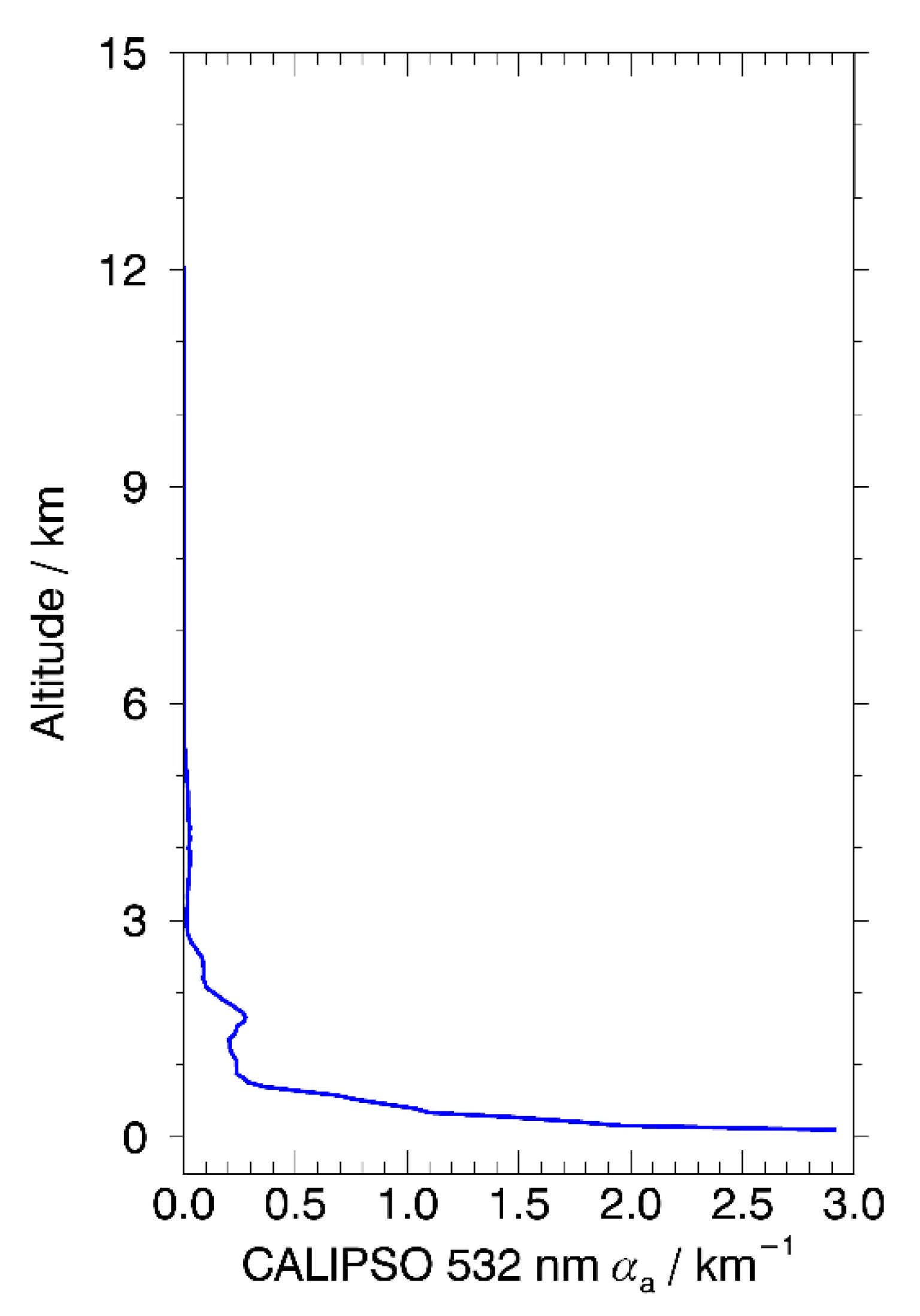
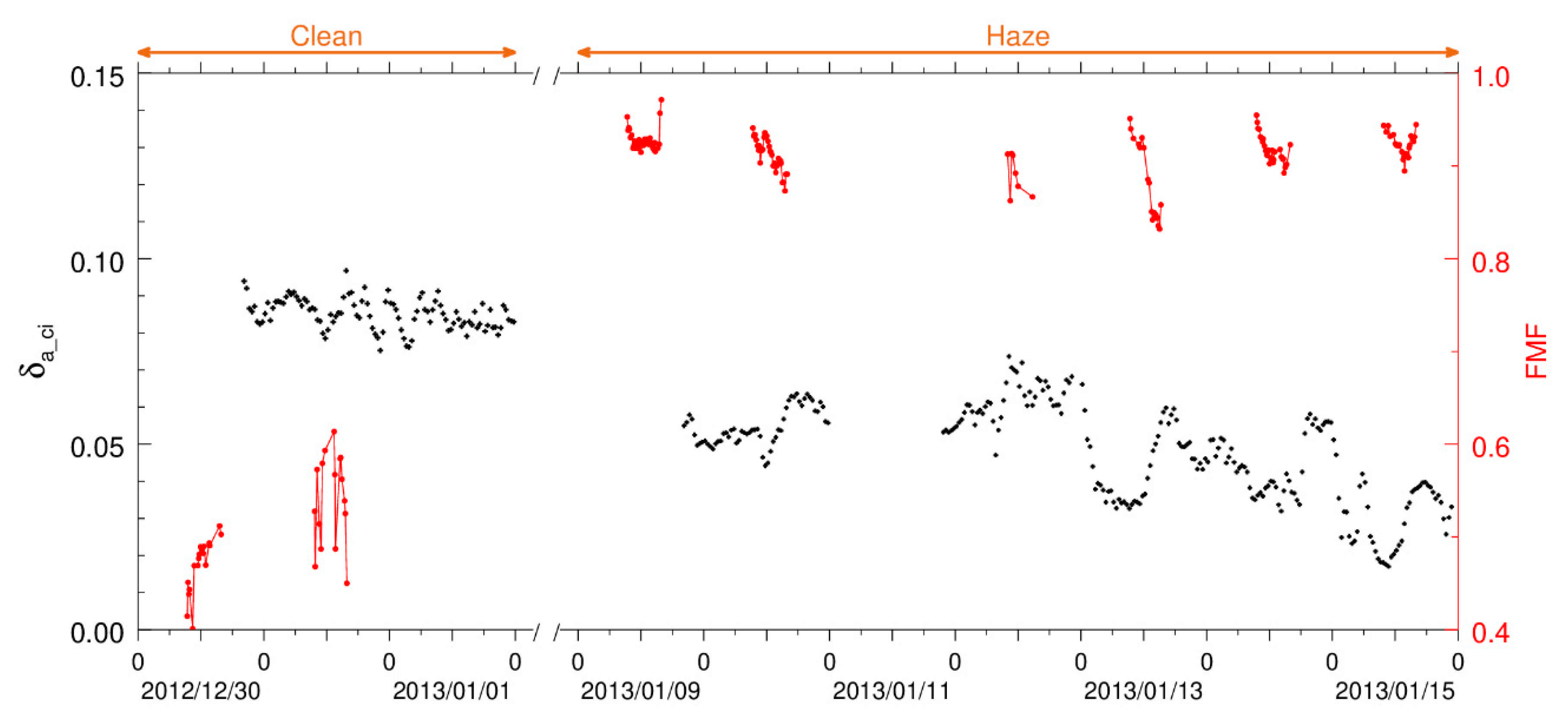
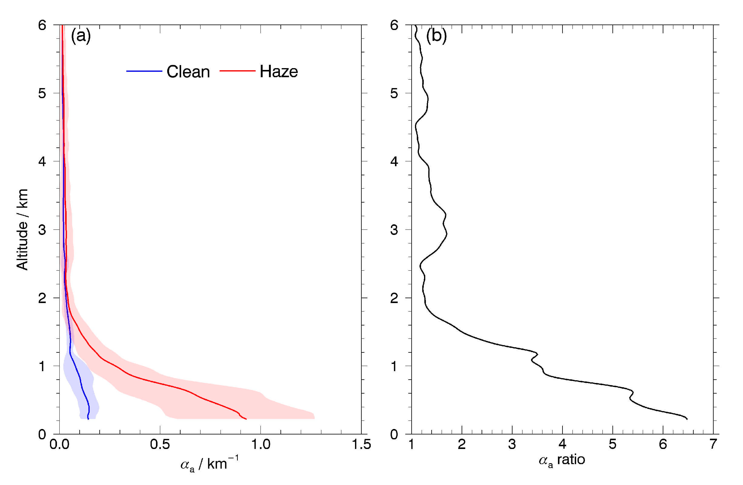
- During the haze period, the integrated particle depolarization ratio was 0.05 ± 0.02, and the fine mode fraction of AOD reached 0.91 ± 0.03. Aerosol extinction peaked near the ground and exhibited a sharp decrease with increasing altitude. These characterizations linked this haze episode intimately with substantial anthropogenic emissions of the local scale;
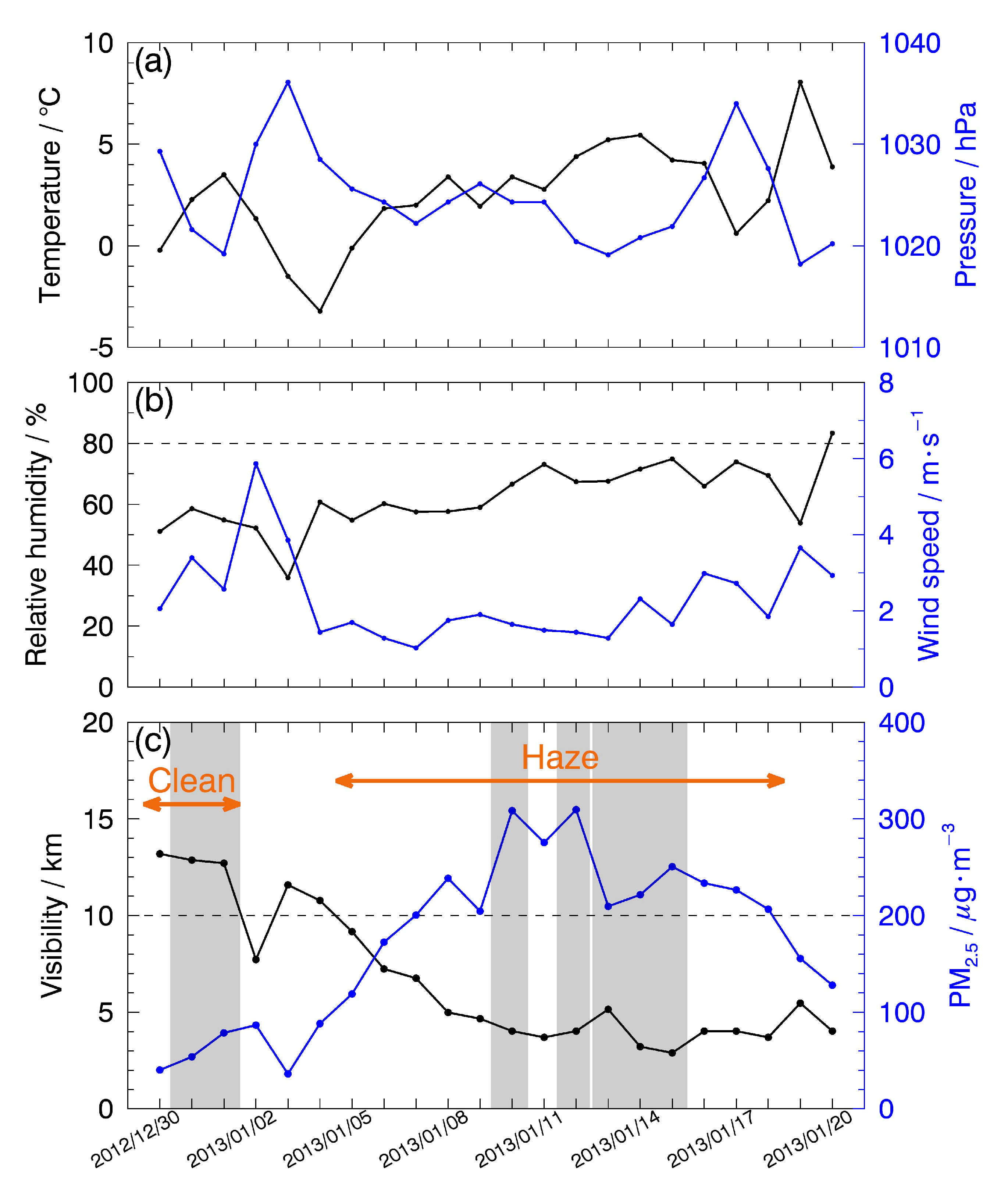
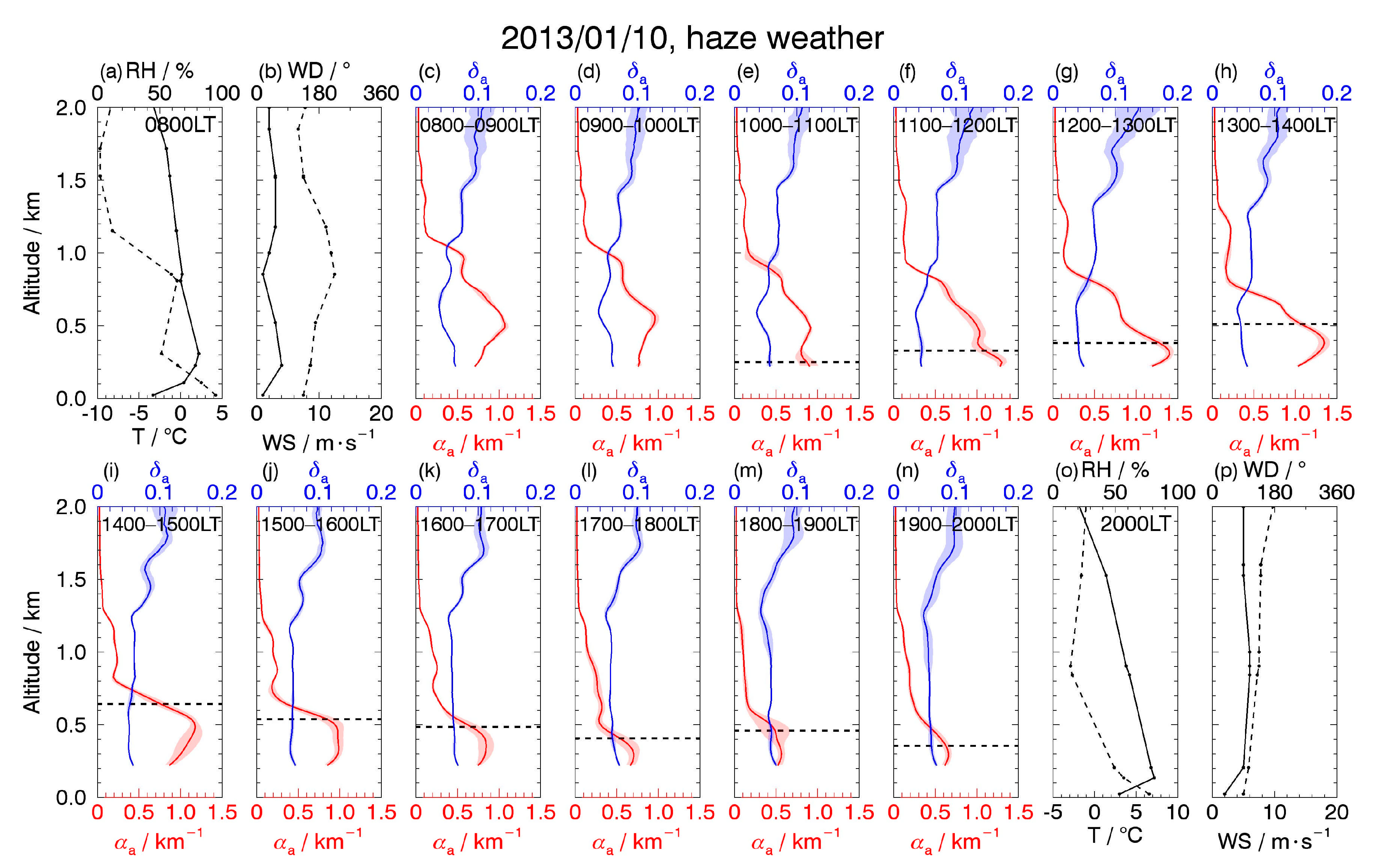
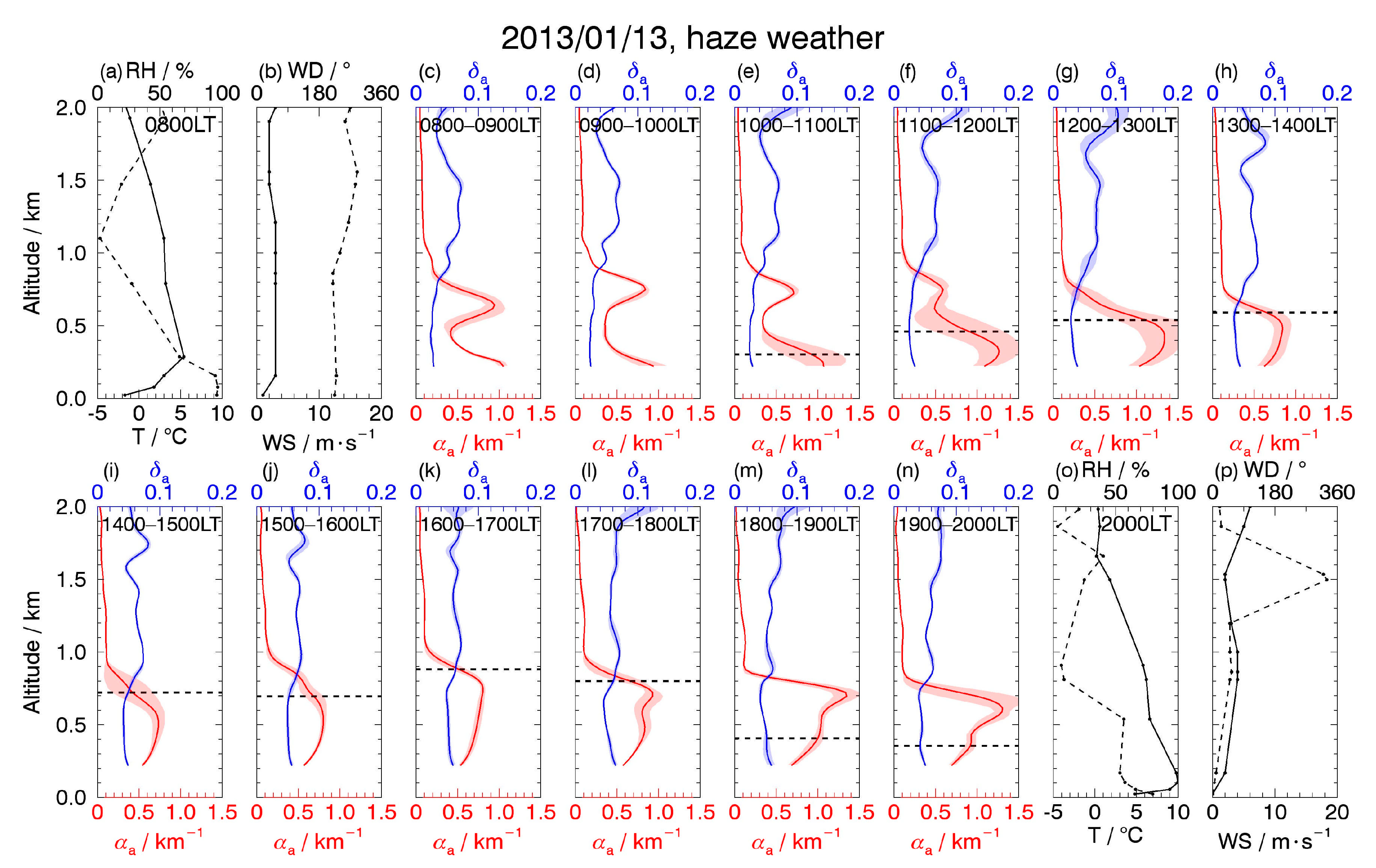
- The daytime evolution of aerosol vertical distribution in the ABL showed a distinct pattern on polluted days. Abundant particles accumulated below 0.5 km in the morning hours due to stable meteorological conditions, including a strong surface-based inversion (4.4–8.1 °C), late development (from 1000–1100 LT) of the convective boundary layer, and weak wind (2.5–3.8 m∙s−1) in the lowermost troposphere. In the afternoon, improved ventilation delivered an overall reduction in boundary layer aerosols but was still insufficient to eliminate haze. Particularly, the morning residual layer had an AOD of between 0.29 and 0.56, serving as the reservoir of aerosol particles. The optically thick residual layer influenced air quality indirectly by weakening convective mixing in the morning hours and directly through the fumigation process around noon, suggesting it may be an important element in aerosol–ABL interactions during consecutive days with haze;
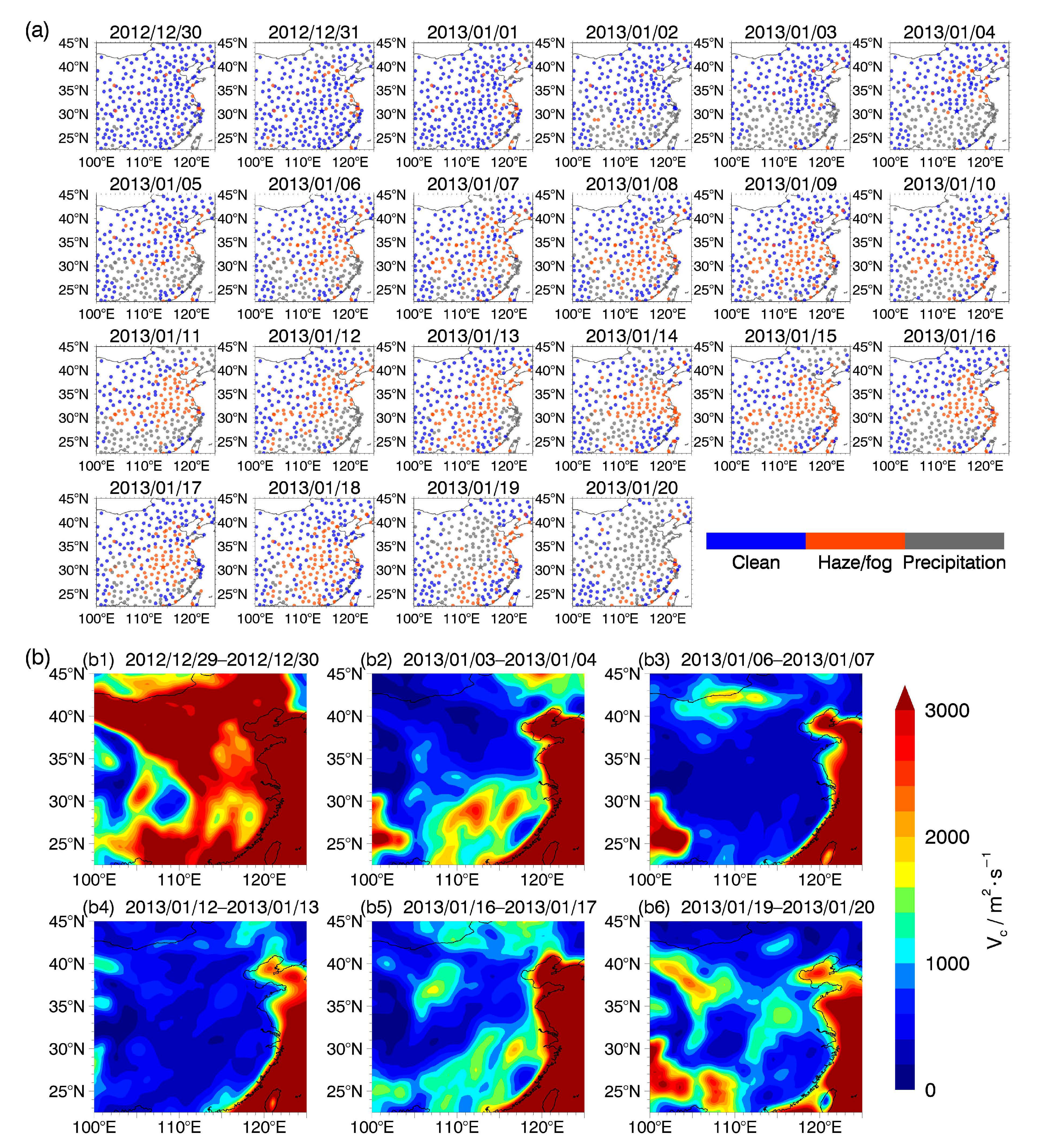
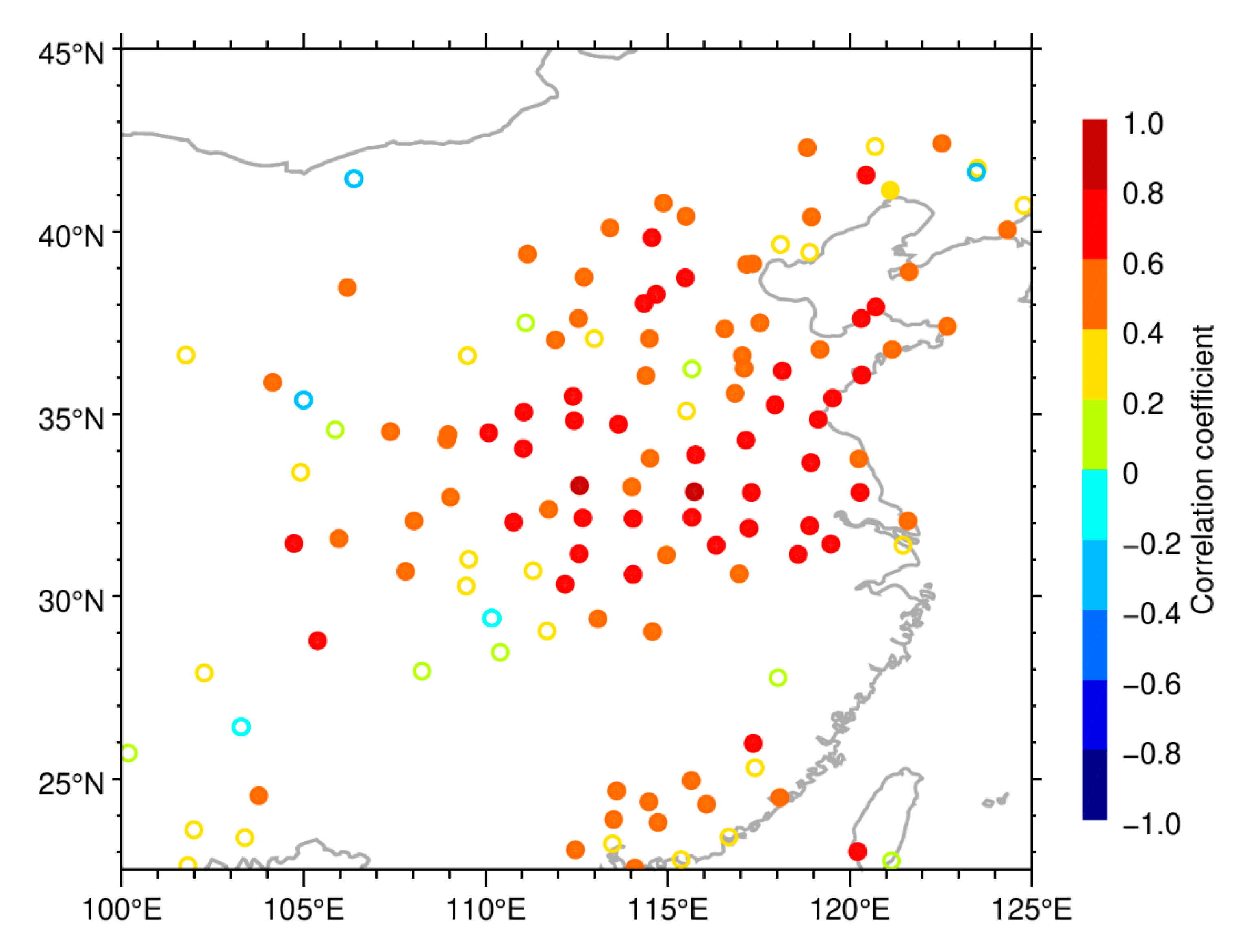
- In January 2013, the positive correlations between the visibility and ventilation coefficients were statistically significant at a 95% confidence level for 72% of the GSOD sites over central and eastern China, linking the large-scale haze episode tightly with poor ventilation. Moreover, the strongest correlations were found over the most polluted area (roughly 111–123° E and 28–40° N, including Wuhan);
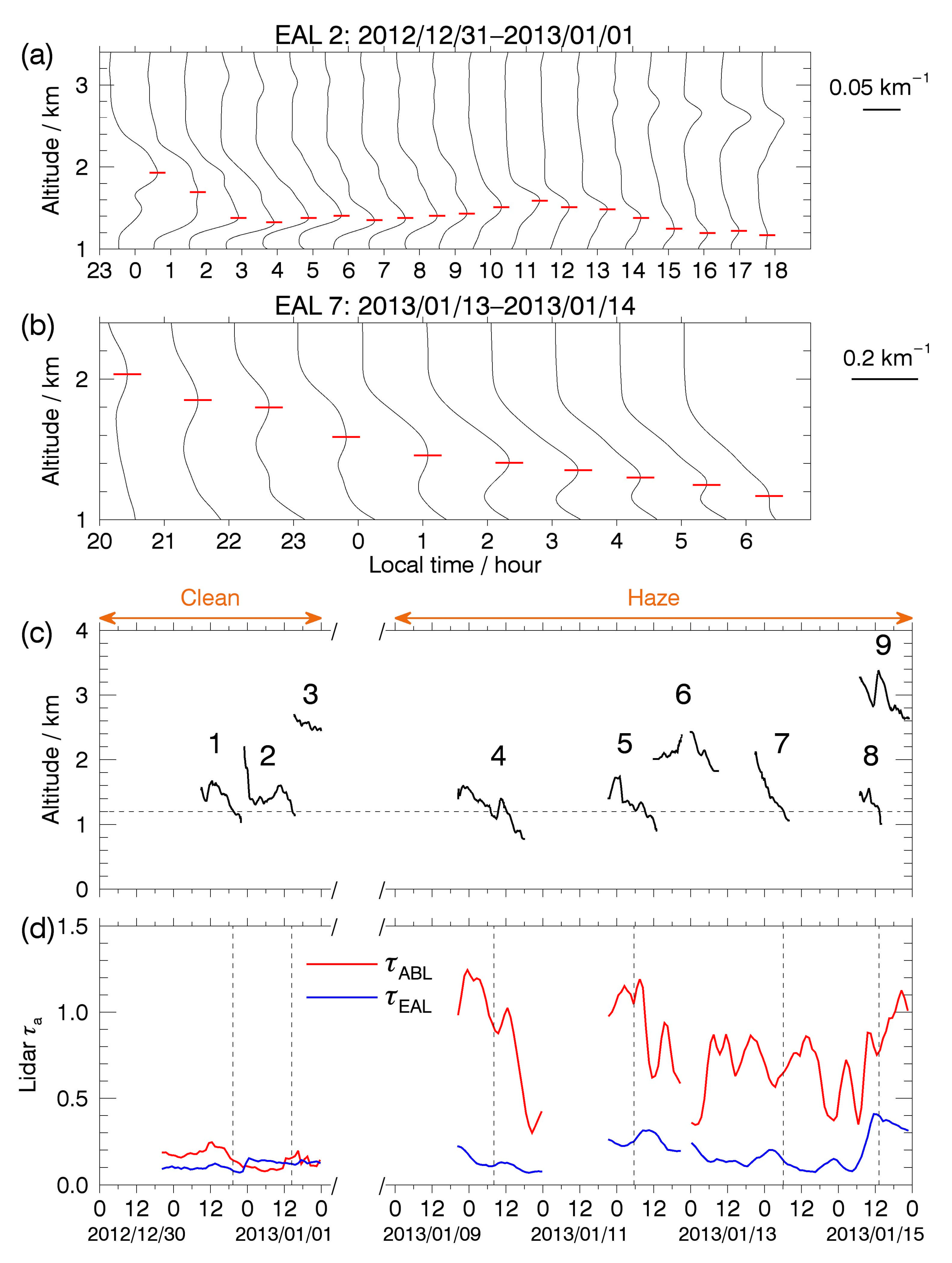
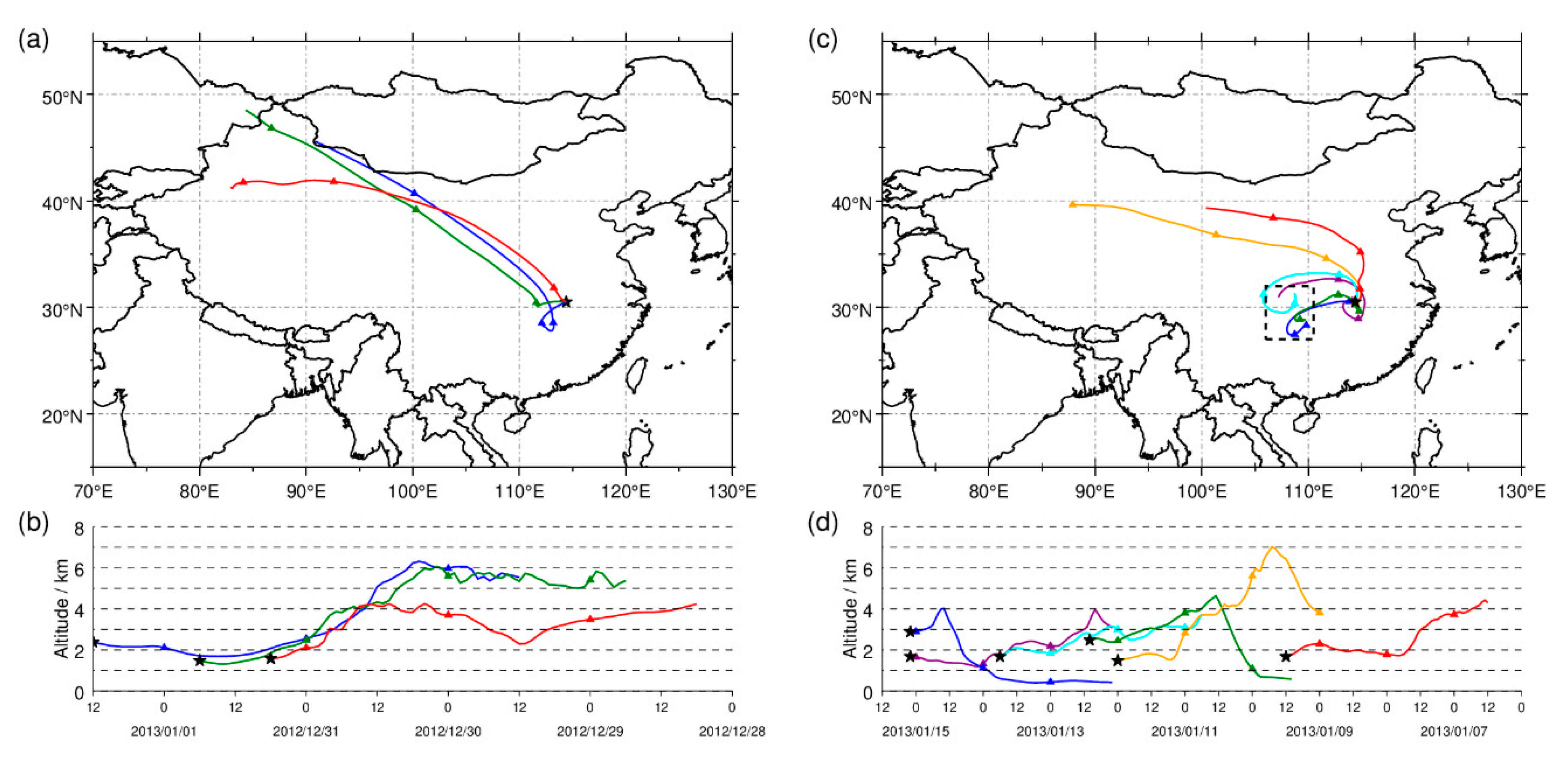
- Most of the lidar-captured elevated aerosol layers (EALs) were observed to subside eventually into the ABL and thereby exacerbate the pollution level. Combined backward trajectory analysis and lidar data revealed the EALs came from the transport of anthropogenic pollutants from the Sichuan Basin, China, and of dust from the Taklamakan and Gobi deserts. We estimated aerosol transport via the two pathways contributed approximately 19% of columnar AOD during the haze episode. Considering the severity and persistence of this haze episode, we suggested aerosol transport play a non-negligible role in the evolution processes of haze.
Author Contributions
Funding
Data Availability Statement
Acknowledgments
Conflicts of Interest
References
- Ding, Y.H.; Liu, Y.J. Analysis of long-term variations of fog and haze in China in recent 50 years and their relations with atmospheric humidity. Sci. China-Earth Sci. 2014, 57, 36–46. [Google Scholar] [CrossRef]
- Zheng, B.; Tong, D.; Li, M.; Liu, F.; Hong, C.P.; Geng, G.N.; Li, H.Y.; Li, X.; Peng, L.Q.; Qi, J.; et al. Trends in China’s anthropogenic emissions since 2010 as the consequence of clean air actions. Atmos. Chem. Phys. 2018, 18, 14095–14111. [Google Scholar] [CrossRef] [Green Version]
- Song, C.B.; Wu, L.; Xie, Y.C.; He, J.J.; Chen, X.; Wang, T.; Lin, Y.C.; Jin, T.S.; Wang, A.X.; Liu, Y.; et al. Air pollution in China: Status and spatiotemporal variations. Environ. Pollut. 2017, 227, 334–347. [Google Scholar] [CrossRef]
- Liu, Z.R.; Hu, B.; Ji, D.S.; Cheng, M.T.; Gao, W.K.; Shi, S.Z.; Xie, Y.Z.; Yang, S.H.; Gao, M.; Fu, H.B.; et al. Characteristics of fine particle explosive growth events in Beijing, China: Seasonal variation, chemical evolution pattern and formation mechanism. Sci. Total Environ. 2019, 687, 1073–1086. [Google Scholar] [CrossRef]
- Zheng, G.J.; Duan, F.K.; Su, H.; Ma, Y.L.; Cheng, Y.; Zheng, B.; Zhang, Q.; Huang, T.; Kimoto, T.; Chang, D.; et al. Exploring the severe winter haze in Beijing: The impact of synoptic weather, regional transport and heterogeneous reactions. Atmos. Chem. Phys. 2015, 15, 2969–2983. [Google Scholar] [CrossRef] [Green Version]
- Wang, Y.S.; Yao, L.; Wang, L.L.; Liu, Z.R.; Ji, D.S.; Tang, G.Q.; Zhang, J.K.; Sun, Y.; Hu, B.; Xin, J.Y. Mechanism for the formation of the January 2013 heavy haze pollution episode over central and eastern China. Sci. China-Earth Sci. 2014, 57, 14–25. [Google Scholar] [CrossRef]
- Gao, M.; Carmichael, G.R.; Wang, Y.; Saide, P.E.; Yu, M.; Xin, J.; Liu, Z.; Wang, Z. Modeling study of the 2010 regional haze event in the North China Plain. Atmos. Chem. Phys. 2016, 16, 1673–1691. [Google Scholar] [CrossRef] [Green Version]
- An, Z.S.; Huang, R.J.; Zhang, R.Y.; Tie, X.X.; Li, G.H.; Cao, J.J.; Zhou, W.J.; Shi, Z.G.; Han, Y.M.; Gu, Z.L.; et al. Severe haze in northern China: A synergy of anthropogenic emissions and atmospheric processes. Proc. Natl. Acad. Sci. USA 2019, 116, 8657–8666. [Google Scholar] [CrossRef] [PubMed] [Green Version]
- Ramanathan, V.; Chung, C.; Kim, D.; Bettge, T.; Buja, L.; Kiehl, J.T.; Washington, W.M.; Fu, Q.; Sikka, D.R.; Wild, M. Atmospheric brown clouds: Impacts on South Asian climate and hydrological cycle. Proc. Natl. Acad. Sci. USA 2005, 102, 5326–5333. [Google Scholar] [CrossRef] [PubMed] [Green Version]
- Navarro, J.C.A.; Varma, V.; Riipinen, I.; Seland, O.; Kirkevag, A.; Struthers, H.; Iversen, T.; Hansson, H.C.; Ekman, A.M.L. Amplification of Arctic warming by past air pollution reductions in Europe. Nat. Geosci. 2016, 9, 277–281. [Google Scholar] [CrossRef]
- Brunekreef, B.; Holgate, S.T. Air pollution and health. Lancet 2002, 360, 1233–1242. [Google Scholar] [CrossRef]
- Pope, C.A., III; Dockery, D.W. Health effects of fine particulate air pollution: Lines that connect. J. Air Waste Manag. Assoc. 2006, 56, 709–742. [Google Scholar] [CrossRef] [PubMed]
- Wolf, T.; Esau, I.; Reuder, J. Analysis of the vertical temperature structure in the Bergen valley, Norway, and its connection to pollution episodes. J. Geophys. Res. Atmos. 2014, 119, 10645–10662. [Google Scholar] [CrossRef] [Green Version]
- Pal, S.; Lee, T.R.; Phelps, S.; De Wekker, S.F.J. Impact of atmospheric boundary layer depth variability and wind reversal on the diurnal variability of aerosol concentration at a valley site. Sci. Total Environ. 2014, 496, 424–434. [Google Scholar] [CrossRef]
- Stull, R.B. An Introduction to Boundary Layer Meteorology; Springer: Berlin/Heidelberg, Germany, 1988; pp. 1–27. [Google Scholar]
- Zhang, R.H.; Li, Q.; Zhang, R.N. Meteorological conditions for the persistent severe fog and haze event over eastern China in January 2013. Sci. China-Earth Sci. 2014, 57, 26–35. [Google Scholar] [CrossRef]
- Petäjä, T.; Järvi, L.; Kerminen, V.M.; Ding, A.J.; Sun, J.N.; Nie, W.; Kujansuu, J.; Virkkula, A.; Yang, X.; Fu, C.B.; et al. Enhanced air pollution via aerosol-boundary layer feedback in China. Sci. Rep. 2016, 6, 18998. [Google Scholar] [CrossRef] [Green Version]
- Quan, J.N.; Gao, Y.; Zhang, Q.; Tie, X.X.; Cao, J.J.; Han, S.Q.; Meng, J.W.; Chen, P.F.; Zhao, D.L. Evolution of planetary boundary layer under different weather conditions, and its impact on aerosol concentrations. Particuology 2013, 11, 34–40. [Google Scholar] [CrossRef]
- Huang, X.; Wang, Z.L.; Ding, A.J. Impact of Aerosol-PBL Interaction on Haze Pollution: Multiyear Observational Evidences in North China. Geophys. Res. Lett. 2018, 45, 8596–8603. [Google Scholar] [CrossRef] [Green Version]
- Li, Z.Q.; Guo, J.P.; Ding, A.J.; Liao, H.; Liu, J.J.; Sun, Y.L.; Wang, T.J.; Xue, H.W.; Zhang, H.S.; Zhu, B. Aerosol and boundary-layer interactions and impact on air quality. Natl. Sci. Rev. 2017, 4, 810–833. [Google Scholar] [CrossRef]
- Su, T.N.; Li, Z.Q.; Li, C.C.; Li, J.; Han, W.C.; Shen, C.Y.; Tan, W.S.; Wei, J.; Guo, J.P. The significant impact of aerosol vertical structure on lower atmosphere stability and its critical role in aerosol-planetary boundary layer (PBL) interactions. Atmos. Chem. Phys. 2020, 20, 3713–3724. [Google Scholar] [CrossRef] [Green Version]
- Zhang, Q.; Ma, X.C.; Tie, X.X.; Huang, M.Y.; Zhao, C.S. Vertical distributions of aerosols under different weather conditions: Analysis of in-situ aircraft measurements in Beijing, China. Atmos. Environ. 2009, 43, 5526–5535. [Google Scholar] [CrossRef]
- Baars, H.; Ansmann, A.; Engelmann, R.; Althausen, D. Continuous monitoring of the boundary-layer top with lidar. Atmos. Chem. Phys. 2008, 8, 7281–7296. [Google Scholar] [CrossRef] [Green Version]
- Kong, W.; Yi, F. Convective boundary layer evolution from lidar backscatter and its relationship with surface aerosol concentration at a location of a central China megacity. J. Geophys. Res. Atmos. 2015, 120, 7928–7940. [Google Scholar] [CrossRef]
- Wang, Z.F.; Li, J.; Wang, Z.; Yang, W.Y.; Tang, X.; Ge, B.Z.; Yan, P.Z.; Zhu, L.L.; Chen, X.S.; Chen, H.S.; et al. Modeling study of regional severe hazes over mid-eastern China in January 2013 and its implications on pollution prevention and control. Sci. China-Earth Sci. 2014, 57, 3–13. [Google Scholar] [CrossRef]
- Qin, K.; Wu, L.X.; Wong, M.S.; Letu, H.; Hu, M.Y.; Lang, H.M.; Sheng, S.J.; Teng, J.Y.; Xiao, X.; Yuan, L.M. Trans-boundary aerosol transport during a winter haze episode in China revealed by ground-based Lidar and CALIPSO satellite. Atmos. Environ. 2016, 141, 20–29. [Google Scholar] [CrossRef] [Green Version]
- Guo, S.; Hu, M.; Zamora, M.L.; Peng, J.F.; Shang, D.J.; Zheng, J.; Du, Z.F.; Wu, Z.; Shao, M.; Zeng, L.M.; et al. Elucidating severe urban haze formation in China. Proc. Natl. Acad. Sci. USA 2014, 111, 17373–17378. [Google Scholar] [CrossRef] [PubMed] [Green Version]
- Li, P.F.; Yan, R.C.; Yu, S.C.; Wang, S.; Liu, W.P.; Bao, H.M. Reinstate regional transport of PM2.5 as a major cause of severe haze in Beijing. Proc. Natl. Acad. Sci. USA 2015, 112, E2739–E2740. [Google Scholar] [CrossRef] [Green Version]
- Wang, Q.Q.; Sun, Y.L.; Xu, W.Q.; Du, W.; Zhou, L.B.; Tang, G.Q.; Chen, C.; Cheng, X.L.; Zhao, X.J.; Ji, D.S.; et al. Vertically resolved characteristics of air pollution during two severe winter haze episodes in urban Beijing, China. Atmos. Chem. Phys. 2018, 18, 2495–2509. [Google Scholar] [CrossRef] [Green Version]
- Onishi, K.; Kurosaki, Y.; Otani, S.; Yoshida, A.; Sugimoto, N.; Kurozawa, Y. Atmospheric transport route determines components of Asian dust and health effects in Japan. Atmos. Environ. 2012, 49, 94–102. [Google Scholar] [CrossRef]
- McKendry, I.; Strawbridge, K.; Karumudi, M.L.; O’Neill, N.; Macdonald, A.M.; Leaitch, R.; Jaffe, D.; Cottle, P.; Sharma, S.; Sheridan, P.; et al. Californian forest fire plumes over Southwestern British Columbia: Lidar, sunphotometry, and mountaintop chemistry observations. Atmos. Chem. Phys. 2011, 11, 465–477. [Google Scholar] [CrossRef] [Green Version]
- Ansmann, A.; Tesche, M.; Gross, S.; Freudenthaler, V.; Seifert, P.; Hiebsch, A.; Schmidt, J.; Wandinger, U.; Mattis, I.; Muller, D.; et al. The 16 April 2010 major volcanic ash plume over central Europe: EARLINET lidar and AERONET photometer observations at Leipzig and Munich, Germany. Geophys. Res. Lett. 2010, 37, 5. [Google Scholar] [CrossRef] [Green Version]
- Zhang, F.; Wang, Z.W.; Cheng, H.R.; Lv, X.P.; Gong, W.; Wang, X.M.; Zhang, G. Seasonal variations and chemical characteristics of PM2.5 in Wuhan, central China. Sci. Total Environ. 2015, 518, 97–105. [Google Scholar] [CrossRef] [PubMed]
- Liu, B.M.; Ma, Y.Y.; Gong, W.; Zhang, M.; Yang, J. Study of continuous air pollution in winter over Wuhan based on ground-based and satellite observations. Atmos. Pollut. Res. 2018, 9, 156–165. [Google Scholar] [CrossRef]
- Zhang, Y.P.; Yi, F.; Kong, W.; Yi, Y. Slope characterization in combining analog and photon count data from atmospheric lidar measurements. Appl. Opt. 2014, 53, 7312–7320. [Google Scholar] [CrossRef] [PubMed]
- Newsom, R.K.; Turner, D.D.; Mielke, B.; Clayton, M.; Ferrare, R.; Sivaraman, C. Simultaneous analog and photon counting detection for Raman lidar. Appl. Opt. 2009, 48, 3903–3914. [Google Scholar] [CrossRef] [PubMed]
- Zhuang, J.; Yi, F. Nabro aerosol evolution observed jointly by lidars at a mid-latitude site and CALIPSO. Atmos. Environ. 2016, 140, 106–116. [Google Scholar] [CrossRef]
- Fernald, F.G. Analysis of atmospheric lidar observations: Some comments. Appl. Opt. 1984, 23, 652–653. [Google Scholar] [CrossRef]
- Klett, J.D. Stable analytical inversion solution for processing lidar returns. Appl. Opt. 1981, 20, 211–220. [Google Scholar] [CrossRef] [Green Version]
- Wang, W.; Gong, W.; Mao, F.Y.; Pan, Z.X.; Liu, B.M. Measurement and Study of Lidar Ratio by Using a Raman Lidar in Central China. Int. J. Environ. Res. Public Health 2016, 13, 13. [Google Scholar] [CrossRef] [Green Version]
- Burton, S.P.; Ferrare, R.A.; Vaughan, M.A.; Omar, A.H.; Rogers, R.R.; Hostetler, C.A.; Hair, J.W. Aerosol classification from airborne HSRL and comparisons with the CALIPSO vertical feature mask. Atmos. Meas. Tech. 2013, 6, 1397–1412. [Google Scholar] [CrossRef] [Green Version]
- Sasano, Y.; Browell, E.V. Light scattering characteristics of various aerosol types derived from multiple wavelength lidar observations. Appl. Opt. 1989, 28, 1670–1679. [Google Scholar] [CrossRef] [PubMed]
- CALIPSO Lidar Level 3 Tropospheric Aerosol Profiles, Cloud Free Data, Standard V4-20; CAL_LID_L3_Tropospheric_APro_CloudFree-Standard-V4-20; NASA/LARC/SD/ASDC: Hampton, VA, USA, 2019.
- Bitar, L.; Duck, T.J.; Kristiansen, N.I.; Stohl, A.; Beauchamp, S. Lidar observations of Kasatochi volcano aerosols in the troposphere and stratosphere. J. Geophys. Res. Atmos. 2010, 115, 10. [Google Scholar] [CrossRef] [Green Version]
- Comerón, A.; Rocadenbosch, F.; López, M.A.; Rodríguez, A.; Muñoz, C.; García-Vizcaíno, D.; Sicard, M. Effects of noise on lidar data inversion with the backward algorithm. Appl. Opt. 2004, 43, 2572–2577. [Google Scholar] [CrossRef] [PubMed] [Green Version]
- Freudenthaler, V.; Esselborn, M.; Wiegner, M.; Heese, B.; Tesche, M.; Ansmann, A.; Muller, D.; Althausen, D.; Wirth, M.; Fix, A.; et al. Depolarization ratio profiling at several wavelengths in pure Saharan dust during SAMUM 2006. Tellus Ser. B Chem. Phys. Meteorol. 2009, 61, 165–179. [Google Scholar] [CrossRef] [Green Version]
- Sassen, K. Polarization in Lidar. In Lidar: Range-Resolved Optical Remote Sensing of the Atmosphere; Weitkamp, C., Ed.; Springer: New York, NY, USA, 2005; pp. 19–42. [Google Scholar]
- Behrendt, A.; Nakamura, T. Calculation of the calibration constant of polarization lidar and its dependency on atmospheric temperature. Opt. Express 2002, 10, 805–817. [Google Scholar] [CrossRef] [PubMed]
- Liu, Z.Y.; Fairlie, T.D.; Uno, I.; Huang, J.F.; Wu, D.; Omar, A.; Kar, J.; Vaughan, M.; Rogers, R.; Winker, D.; et al. Transpacific transport and evolution of the optical properties of Asian dust. J. Quant. Spectrosc. Radiat. Transf. 2013, 116, 24–33. [Google Scholar] [CrossRef]
- Sakai, T.; Nagai, T.; Zaizen, Y.; Mano, Y. Backscattering linear depolarization ratio measurements of mineral, sea-salt, and ammonium sulfate particles simulated in a laboratory chamber. Appl. Opt. 2010, 49, 4441–4449. [Google Scholar] [CrossRef]
- Müller, D.; Ansmann, A.; Mattis, I.; Tesche, M.; Wandinger, U.; Althausen, D.; Pisani, G. Aerosol-type-dependent lidar ratios observed with Raman lidar. J. Geophys. Res. Atmos. 2007, 112. [Google Scholar] [CrossRef]
- Dieudonne, E.; Chazette, P.; Marnas, F.; Totems, J.; Shang, X. Raman Lidar Observations of Aerosol Optical Properties in 11 Cities from France to Siberia. Remote Sens. 2017, 9, 978. [Google Scholar] [CrossRef] [Green Version]
- Shaw, G.E. Sun Photometry. Bull. Amer. Meteorol. Soc. 1983, 64, 4–10. [Google Scholar] [CrossRef] [Green Version]
- Holben, B.N.; Eck, T.F.; Slutsker, I.; Tanre, D.; Buis, J.P.; Setzer, A.; Vermote, E.; Reagan, J.A.; Kaufman, Y.J.; Nakajima, T.; et al. AERONET—A federated instrument network and data archive for aerosol characterization. Remote Sens. Environ. 1998, 66, 1–16. [Google Scholar] [CrossRef]
- Eck, T.F.; Holben, B.N.; Reid, J.S.; Dubovik, O.; Smirnov, A.; O’Neill, N.T.; Slutsker, I.; Kinne, S. Wavelength dependence of the optical depth of biomass burning, urban, and desert dust aerosols. J. Geophys. Res. Atmos. 1999, 104, 31333–31349. [Google Scholar] [CrossRef]
- Smirnov, A.; Holben, B.N.; Eck, T.F.; Dubovik, O.; Slutsker, I. Cloud-screening and quality control algorithms for the AERONET database. Remote Sens. Environ. 2000, 73, 337–349. [Google Scholar] [CrossRef]
- O’Neill, N.T.; Dubovik, O.; Eck, T.F. Modified Ångström exponent for the characterization of submicrometer aerosols. Appl. Opt. 2001, 40, 2368–2375. [Google Scholar] [CrossRef]
- O’Neill, N.T.; Eck, T.F.; Smirnov, A.; Holben, B.N.; Thulasiraman, S. Spectral discrimination of coarse and fine mode optical depth. J. Geophys. Res. Atmos. 2003, 108, 15. [Google Scholar] [CrossRef]
- National Centers for Environmental Information. Global Surface Summary of the Day—GSOD. Available online: https://www.ncei.noaa.gov/access/search/dataset-search (accessed on 30 December 2020).
- Hou, S.Q.; Tong, S.R.; Ge, M.F.; An, J.L. Comparison of atmospheric nitrous acid during severe haze and clean periods in Beijing, China. Atmos. Environ. 2016, 124, 199–206. [Google Scholar] [CrossRef]
- Liu, X.G.; Gu, J.W.; Li, Y.P.; Cheng, Y.F.; Qu, Y.; Han, T.T.; Wang, J.L.; Tian, H.Z.; Chen, J.; Zhang, Y.H. Increase of aerosol scattering by hygroscopic growth: Observation, modeling, and implications on visibility. Atmos. Res. 2013, 132, 91–101. [Google Scholar] [CrossRef]
- Hersbach, H.; Bell, B.; Berrisford, P.; Hirahara, S.; Horanyi, A.; Munoz-Sabater, J.; Nicolas, J.; Peubey, C.; Radu, R.; Schepers, D.; et al. The ERA5 global reanalysis. Q. J. R. Meteorol. Soc. 2020, 1–51. [Google Scholar] [CrossRef]
- Deng, T.; Wu, D.; Deng, X.J.; Tan, H.B.; Li, F.; Liao, B.T. A vertical sounding of severe haze process in Guangzhou area. Sci. China Earth Sci. 2014, 57, 2650–2656. [Google Scholar] [CrossRef]
- Holzworth, G.C. Mixing Depths, Wind Speeds and Air Pollution Potential for Selected Locations in the United States. J. Appl. Meteorol. 1967, 6, 1039–1044. [Google Scholar] [CrossRef] [Green Version]
- Rigby, M.; Timmis, R.; Toumi, R. Similarities of boundary layer ventilation and particulate matter roses. Atmos. Environ. 2006, 40, 5112–5124. [Google Scholar] [CrossRef]
- Stein, A.F.; Draxler, R.R.; Rolph, G.D.; Stunder, B.J.B.; Cohen, M.D.; Ngan, F. NOAA’s HYSPLIT Atmospheric Transport and Dispersion Modeling System. Bull. Amer. Meteorol. Soc. 2015, 96, 2059–2077. [Google Scholar] [CrossRef]
- Huang, J.; Minnis, P.; Chen, B.; Huang, Z.W.; Liu, Z.Y.; Zhao, Q.Y.; Yi, Y.H.; Ayers, J.K. Long-range transport and vertical structure of Asian dust from CALIPSO and surface measurements during PACDEX. J. Geophys. Res. Atmos. 2008, 113, 13. [Google Scholar] [CrossRef]
- Ångström, A. On the Atmospheric Transmission of Sun Radiation and on Dust in the Air. Geogr. Ann. 1929, 11, 156–166. [Google Scholar] [CrossRef]
- Friedlander, S.K. Smoke, Dust, and Haze: Fundamentals of Aerosol Dynamics; Oxford University Press: New York, NY, USA, 2000; pp. 59–124. [Google Scholar]
- Vaughan, M.A.; Powell, K.A. CALIOP Algorithm Theoretical Basis Document Part. 2: Feature Detection and Layer Properties Algorithms; PC-SCI-202 Part 2; NASA: Washington, DC, USA, 2005; pp. 1–87. [Google Scholar]
- Noh, Y.; Müller, D.; Lee, K.; Kim, K.; Lee, K.; Shimizu, A.; Sano, I.; Park, C.B. Depolarization ratios retrieved by AERONET sun–sky radiometer data and comparison to depolarization ratios measured with lidar. Atmos. Chem. Phys. 2017, 17, 6271–6290. [Google Scholar] [CrossRef] [Green Version]
- He, Y.; Yi, F. Dust Aerosols Detected Using a Ground-Based Polarization Lidar and CALIPSO over Wuhan (30.5° N, 114.4° E), China. Adv. Meteorol. 2015, 18. [Google Scholar] [CrossRef]
- Qin, K.; Wang, L.Y.; Xu, J.; Letu, H.S.; Zhang, K.F.; Li, D.; Zou, J.H.; Fan, W.Z. Haze Optical Properties from Long-Term Ground-Based Remote Sensing over Beijing and Xuzhou, China. Remote Sens. 2018, 10, 518. [Google Scholar] [CrossRef] [Green Version]
- Bi, J.R.; Huang, J.P.; Hu, Z.Y.; Holben, B.N.; Guo, Z.Q. Investigating the aerosol optical and radiative characteristics of heavy haze episodes in Beijing during January of 2013. J. Geophys. Res. Atmos. 2014, 119, 9884–9900. [Google Scholar] [CrossRef]
- Haywood, J.M.; Shine, K.P. Multi-spectral calculations of the direct radiative forcing of tropospheric sulphate and soot aerosols using a column model. Q. J. R. Meteorol. Soc. 1997, 123, 1907–1930. [Google Scholar] [CrossRef]
- Wang, H.; Tan, S.C.; Wang, Y.; Jiang, C.; Shi, G.Y.; Zhang, M.X.; Che, H.Z. A multisource observation study of the severe prolonged regional haze episode over eastern China in January 2013. Atmos. Environ. 2014, 89, 807–815. [Google Scholar] [CrossRef]
- Tao, M.H.; Chen, L.F.; Xiong, X.Z.; Zhang, M.G.; Ma, P.F.; Tao, J.H.; Wang, Z.F. Formation process of the widespread extreme haze pollution over northern China in January 2013: Implications for regional air quality and climate. Atmos. Environ. 2014, 98, 417–425. [Google Scholar] [CrossRef]
- Lu, C.; Deng, Q.-H.; Liu, W.-W.; Huang, B.-L.; Shi, L.-Z. Characteristics of ventilation coefficient and its impact on urban air pollution. J. Cent. South. Univ. Technol. 2012, 19, 615–622. [Google Scholar] [CrossRef]
- Sun, K.; Liu, H.N.; Ding, A.J.; Wang, X.Y. WRF-Chem Simulation of a Severe Haze Episode in the Yangtze River Delta, China. Aerosol Air Qual. Res. 2016, 16, 1268–1283. [Google Scholar] [CrossRef] [Green Version]
- Zhang, X.Y.; Wang, Y.Q.; Niu, T.; Zhang, X.C.; Gong, S.L.; Zhang, Y.M.; Sun, J.Y. Atmospheric aerosol compositions in China: Spatial/temporal variability, chemical signature, regional haze distribution and comparisons with global aerosols. Atmos. Chem. Phys. 2012, 12, 779–799. [Google Scholar] [CrossRef] [Green Version]
- Ma, Y.J.; Ye, J.H.; Xin, J.Y.; Zhang, W.Y.; de Arellano, J.V.G.; Wang, S.G.; Zhao, D.D.; Dai, L.D.; Ma, Y.X.; Wu, X.Y.; et al. The Stove, Dome, and Umbrella Effects of Atmospheric Aerosol on the Development of the Planetary Boundary Layer in Hazy Regions. Geophys. Res. Lett. 2020, 47, 10. [Google Scholar] [CrossRef]
- Zhang, J.S.; Chen, Z.Y.; Lu, Y.H.; Gui, H.Q.; Liu, J.G.; Liu, W.Q.; Wang, J.; Yu, T.Z.; Cheng, Y.; Chen, Y.; et al. Characteristics of aerosol size distribution and vertical backscattering coefficient profile during 2014 APEC in Beijing. Atmos. Environ. 2017, 148, 30–41. [Google Scholar] [CrossRef]
- Fan, W.Z.; Qin, K.; Xu, J.; Yuan, L.M.; Li, D.; Jin, Z.; Zhang, K.F. Aerosol vertical distribution and sources estimation at a site of the Yangtze River Delta region of China. Atmos. Res. 2019, 217, 128–136. [Google Scholar] [CrossRef] [Green Version]


| Parameter | Specification |
|---|---|
| Transmitter | |
| Laser model | Continuum Inlite II-20 |
| Wavelength | 532 nm |
| Energy per pulse | ~60 mJ |
| Pulse repetition rate | 20 Hz |
| Pulse width | 5–7 ns |
| Beam divergence | ~0.2 mrad |
| Receiver | |
| Telescope | Cassegrain |
| Primary mirror diameter | 200 mm |
| Field of view | 1.0 mrad |
| PBS | Tp > 95%, Rs > 99% |
| Filter bandwidth | 0.3 nm |
| PMT | Hamamatsu H10721 |
| Other | |
| Acquisition model | Licel TR40-160 |
| Positioning | 29° off zenith |
| Date | 0.2 km αa (km−1) | ∆T a (°C) | WS b (m∙s−1) | τRL | TCBL c | SDSR d (Wh∙m−2) | CBLHmax e (km) | ||
|---|---|---|---|---|---|---|---|---|---|
| 0800 LT | 2000 LT | 0800 LT | 2000 LT | ||||||
| Clear | |||||||||
| 31 December 2012 | 0.14 ± 0.03 | 3.3 | 3.0 | 8.2 | 9.0 | 0.13 ± 0.01 | 0800 LT | 2525 | 1.09 |
| 1 January 2013 | 0.12 ± 0.05 | 5.7 | 3.6 | 6.1 | 6.0 | 0.05 ± 0.01 | 0800 LT | 3167 | 0.88 |
| Haze | |||||||||
| 10 January 2013 | 0.84 ± 0.25 | 5.5 | 4.2 | 2.5 | 5.4 | 0.56 ± 0.02 | 1000 LT | 944 | 0.64 |
| 12 January 2013 | 1.14 ± 0.47 | 5.9 | 2.2 | 3.6 | 3.0 | 0.38 ± 0.04 | 1100 LT | 550 | 0.48 |
| 13 January 2013 | 0.73 ± 0.30 | 7.1 | 5.2 | 2.8 | 3.3 | 0.41 ± 0.05 | 1000 LT | 1225 | 0.88 |
| 14 January 2013 | 0.70 ± 0.26 | 8.1 | 4.6 | 3.8 | 7.1 | 0.34 ± 0.03 | 1000 LT | 1169 | 0.7 |
| 15 January 2013 | 0.89 ± 0.36 | 4.4 | 3.2 | 3.2 | 2.5 | 0.29 ± 0.04 | 1000 LT | 778 | 0.51 |
| Index | Lidar-Detected EAL | HYSPLIT Backward Trajectory | ||
|---|---|---|---|---|
| αa Maximum (km−1) | a | Airflow Direction | Trajectory Length (km) | |
| Clear | ||||
| 1 | 0.08 | 0.11 ± 0.01 | Northwest | 3211 |
| 2 | 0.10 | 0.11 ± 0.01 | Northwest | 3385 |
| 3 | 0.10 | 0.10 ± 0.02 | Northwest | 3311 |
| Haze | ||||
| 4 | 0.32 | 0.09 ± 0.02 | Northwest | 1952 |
| 5 | 0.41 | 0.08 ± 0.03 | Northwest | 2806 |
| 6 | 0.16 | 0.02 ± 0.01 | West | 1027 |
| 7 | 0.29 | 0.05 ± 0.01 | West | 1679 |
| 8 | 0.43 | 0.04 ± 0.01 | West | 1513 |
| 9 | 0.26 | 0.01 ± 0.01 | West | 1056 |
Publisher’s Note: MDPI stays neutral with regard to jurisdictional claims in published maps and institutional affiliations. |
© 2021 by the authors. Licensee MDPI, Basel, Switzerland. This article is an open access article distributed under the terms and conditions of the Creative Commons Attribution (CC BY) license (http://creativecommons.org/licenses/by/4.0/).
Share and Cite
Zhang, Y.; Zhang, Y.; Yu, C.; Yi, F. Evolution of Aerosols in the Atmospheric Boundary Layer and Elevated Layers during a Severe, Persistent Haze Episode in a Central China Megacity. Atmosphere 2021, 12, 152. https://doi.org/10.3390/atmos12020152
Zhang Y, Zhang Y, Yu C, Yi F. Evolution of Aerosols in the Atmospheric Boundary Layer and Elevated Layers during a Severe, Persistent Haze Episode in a Central China Megacity. Atmosphere. 2021; 12(2):152. https://doi.org/10.3390/atmos12020152
Chicago/Turabian StyleZhang, Yunfei, Yunpeng Zhang, Changming Yu, and Fan Yi. 2021. "Evolution of Aerosols in the Atmospheric Boundary Layer and Elevated Layers during a Severe, Persistent Haze Episode in a Central China Megacity" Atmosphere 12, no. 2: 152. https://doi.org/10.3390/atmos12020152