High-Resolution Simulation of Polar Lows over Norwegian and Barents Seas Using the COSMO-CLM and ICON Models for the 2019–2020 Cold Season

Abstract

The lack of meteorological observations at high latitudes and the small size and relatively short lifetime of polar lows (PLs) constitute a problem in the simulation and prediction of these phenomena by numerical models. On the other hand, PLs, which are rapidly developing, can lead to such extreme weather events as stormy waves, strong winds, the icing of ships, and snowfalls with low visibility, which can influence communication along the Arctic seas. This article is devoted to studying the possibility of the numerical simulation and prediction of polar lows by different model configurations and resolutions. The results of the numerical experiments for the Norwegian and Barents seas with grid spacings of 6.5 and 2 km using the ICON-Ru configurations of the ICON (ICOsahedral Nonhydrostatic) model and with a grid spacing of 6.5 km using the COSMO-CLM (Climate Limited-area Modeling) configuration of the COSMO (COnsortium for Small-scale MOdelling) model are presented for the cold season of 2019–2020. All the used model configurations demonstrated the possibility of the realistic simulation of polar lows. The ICON model showed slightly more accurate results for the analyzed cases. The best results showed runs with lead times of less than a day.

1. Introduction

For quite a long time, various definitions of polar mesocyclones and polar lows have been used in the literature. The European Polar Low Working Group (EPLWG) defines the term “mesoscale cyclone” or “mesocyclone” (MC) for all polar cyclones poleward of the main polar front having scales smaller than 2000 km. The classical “polar low” (PL) is included as a subtype that is restricted to maritime systems with near-surface winds exceeding 15 m/s [1]. The most well-known definition of a polar low was formulated by Rasmussen and Turner (2003): “A polar low is a small, but fairly intense maritime cyclone that forms poleward of the main baroclinic zone (the polar front or other major baroclinic zone). The horizontal scale of the polar low is approximately between 200 and 1000 km and has surface winds near or above gale force” [2].

The sizes of these mesocyclones are small compared to extratropical cyclones and range from several tens to several hundreds of kilometers [2,3,4]. Intense polar lows cause extreme weather events which develop suddenly and over a short period. Due to the small size of polar lows and their short lifetimes (in most cases, less than a day), sometimes they cannot be observed on synoptic maps. The difficulty of detecting them is more complicated in comparison with standard meteorological observations at high latitudes over the sea.

Several polar cyclone databases have been created over the past two decades. The 10-year Sea Surface Temperature and Altimeter Synergy for Improved Forecasting of Polar Lows project (STARS) is one of the largest and covers the period of 2002–2011. The STARS project presents the most complete dataset for the study of polar lows formed in the period from 2002 to 2011. The work [5] presents the dates of formation and the characteristics of polar lows (PLs) over the North European Basin and the Kara Sea in the period 1981–2002. The characteristics of PLs over the North European Basin were analyzed using cloud cover distribution data for 1981–1995 in the work [6]. In the work [7], data are presented on the climatology of polar mesocyclones over the North and Barents seas for 14 seasons (1995/1996–2008/2009). In [8,9], an objective global climatology of the polar lows was developed; it is based on ERA-I data and covers the period from 1979 to 2016. The second climatology of the PLs was developed on the basis of a more detailed reanalysis for the Arctic (ASR) (grid spacing 15 km) for the period from 2000 to 2012. Due to the existing differences in the definition of polar lows, different databases have different numbers of PLs. For example, the database presented in [7] has a significantly larger number of PLs than the STARS project. This is very interesting, but only for the investigations the new third climatology of the PLs for the North Atlantic PLs for the period from 1979 to 2018 [10]. This dataset was received by the Russian Academy of Sciences North Atlantic Atmospheric Downscaling (RAS-NAAD) project, which provides a 40-y 3D hindcast of the North Atlantic (10°–80° N) atmosphere at a 14 km grid spacing with 50 levels in the vertical direction (up to 50 hPa), performed with a regional setting of the WRF-ARW 3.8.1 model forced by ERA-Interim as a lateral boundary condition.

Reanalysis is one of the sources of PLs data. Various cyclone tracking methods are used to identify PLs based on the identification of certain parameters from the reanalysis databases. However, PLs in different reanalyses are only partially detected due to their insufficient spatial resolution. Some works [11,12,13] have demonstrated a significant underestimation of both the number of PLs and the wind speed in modern reanalysis. In the work [14], a conceptually new approach was developed for detecting PLs based on the use of deep convolutional neural networks.

In [15], it is shown that the adequate identification of PLs, their tracking, and the study of their parameters based on reanalysis data require the use of surface in situ and satellite data and the results of high-resolution atmospheric models. The study [15] demonstrated the possibility of the ensemble forecasting of PLs with a high resolution (grid spacing 4 km) a decade ago. The authors used the UMEPS ensemble system and came to the conclusion that the forecast quality significantly depends on the chosen domain and the model parameterization of physical processes. [16] indicates that with a short-range, high-resolution UMEPS, potentially valuable warnings of extreme weather can be given up to two days in advance.

Attempts to reproduce PLs using high-resolution regional models were made in the early 21st century. For example, in [17] numerical experiments were carried out to reproduce the polar mesocyclone over the Labrador Sea using the MM5 model with nested grids with different grid spacings (60, 20, 6.5 km). Models with coarser grid spacing were used to analyze PL cases at the end of the 20th century. For example, in [18] a mesoscale Canadian model with a grid spacing of 15 km was used for this purpose, and in [19] models with grid spacings of 25 km and 50 km were used. In [20], attempts were made to compare model simulation to observations for a polar low case study highlighting certain model performance and caveats.

The THORPEX (The Observing System Research and Predictability Experiment) cluster was conducted in 2008 in the framework of the International Polar Year (IPY-THORPEX). It included, in particular, additional observations which provided invaluable data for validating models predicting PLs. The most studied case of polar lows is the vortex that appeared in the North Atlantic on 3–4 March 2008. In [21], this PL was analyzed using radiosonde data, satellite imagery, and High-Resolution Limited-Area Model (HIRLAM) forecasts. In [22] and [23], the WRF model with grid spacings of 2 and 3 km, respectively, was used to study the same case. In [24], the dependence of the forecast quality of the PL on the grid spacing was assessed using the Met Office Unified Model. Versions of the model with grid spacings of 12, 4, and 1 km were used. The scientists found that the 4-km version was significantly better than the 12-km version, while modelling with a 1 km resolution did not improve the reproduction of the PL. In a recent work [25], the data from IPY THORPEX were also used to validate two high-resolution models, AROME-Arctic and global model ECMWF, with horizontal grid spacings of 2.5 and 25 km, respectively.

Data from the Year of Polar Prediction (YOPP) Special Observing Period Northern Hemisphere 1 (from 1 February to 31 March, 2018) were used to validate and compare four models, including one global model—the high-resolution version of the ECMWF Integrated Forecasting System (IFS-HRES)—and three regional models: the (AROME) Arctic, the Canadian Arctic Prediction System (CAPS), and the AROME with a Météo-France setup (MF-AROME). The results of this comparison are presented in [26]. A number of other works have been devoted to studying the effects of model parameter variations on the formation of PLs. For example, the work [27] investigated the effect of surface ocean temperature on the occurrence of polar lows. [28,29] estimates how PL forecasting depends on the boundary of the sea ice and the position of the jet stream. In [30], the roles of sea ice and orography in the formation of PLs were investigated. The work [31] investigated the possibility of giving forecasts for the Arctic with the configuration COSMO-Ru (grid spacings of 6.6 and 2.2 km) of the model COSMO. It was shown that the model with a grid spacing of about 2 km was more successful in the simulation of the evaluation and the PLs than the same model with coarser grids at same time sea temperature, and its evaluation during simulation can play a decisive role in the generation of small vortices. In [32], the influence of the parameterization of the planetary boundary layer on the reproduction and evolution of PLs was studied using the WRF model. While the ability of the COSMO model to reproduce PLs has been demonstrated more than once [28,29,31], no similar work has been carried out with the ICON model. ICON is a new model of the German weather service which is also used in Russia. ICON dynamic core tests and other validation assessments showed good results. It is very likely that forecast services currently using COSMO will migrate to ICON in the near future. Therefore, it seems to us very important to compare the capabilities of these two models in predicting PL and to evaluate the predictive capabilities of ICON itself with different grid steps.

Previous studies using the COSMO model focused on the various factors of polar lows formation, such as sea surface temperature, the presence and position of the ice edge, the strength and presence of a jet stream in one or two PL cases [28,29,31]. In our work, in contrast to previous works, we considered seven polar lows cases which appeared in the Norwegian and Barents Seas last winter. While we did not pay much attention to the factors of PL formation, which are considered in earlier works, we investigated the dependence of the forecast the lead time and on the model grid steps.

The purpose of this work was to assess the forecasting capability and resolution sensitivity of the COSMO-CLM and ICON models, as well as reveal their modelling features—in particular, the dependence of the forecasts of polar lows on the lead time. At the first stage, COSMO-CLM and ICON forecasts with a resolution of 6.6 km were compared; at the second stage, versions of the ICON model with grid spacings of 2 and 6.6 km were compared. The model forecasts were validated by comparing them with observational data—i.e., with the data delivered from the ERA5 reanalysis data and the ASCAT data (Advanced Scatterometer) [33]. Numerical experiments were carried out for the cases of PLs detected during the cold period of 2019–2020.

2. Methods

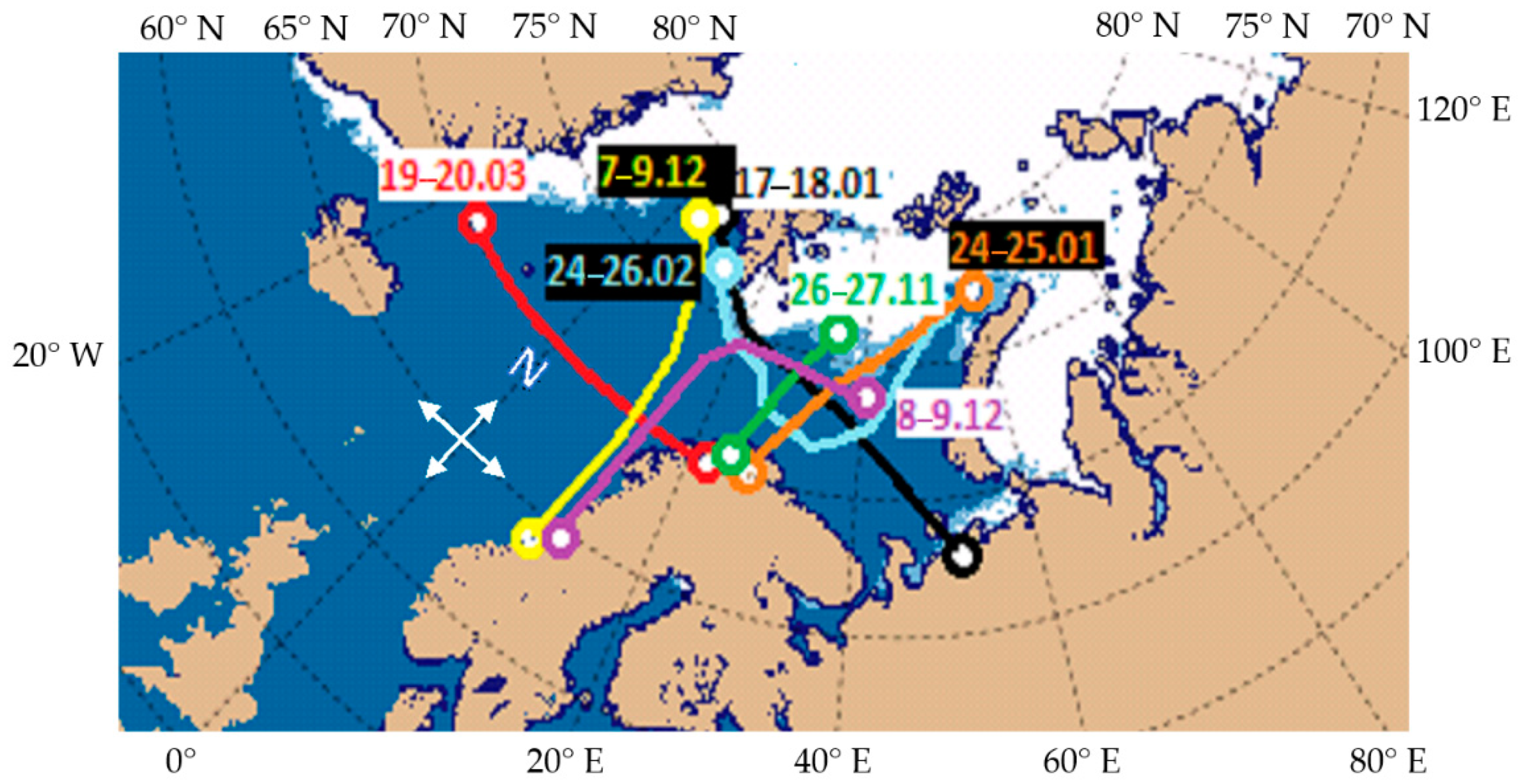
2.1. Geographical Area of Research

Among multiple mesoscale cyclones observed over the world at high and relatively low latitudes, polar lows may significantly impact the operations of the Norwegian and Barents seas, including shipping and aviation traffic lanes and oil and gas field operations. These determine the selection of the Norwegian and Barents seas as areas of the more frequent generation and evolution of PLs in the Arctic area.

We have identified seven well-developed PLs by the daily analysis of satellite images during the cold period of 2019–2020 (November–March) in the area from Greenland to the Norwegian and Barents seas. In [7], it was noted that marine cold-air outbreaks (MCAOs) are required for a cyclone to be classified as a PL. We partly take this into account in the widely applied static stability criterion, where a difference between the sea-surface temperature (SST) and the overlying atmospheric temperature at 500 hPa and/or at 700 hPa should exceed certain thresholds. We apply these criteria for our selected PL cases in Section 3. The area of investigation with the trajectories of the identified PLs is presented in Figure 1.

2.2. Models

In this work, we have used the COSMO-CLM and ICON Limited-Area model (LAM) [34,35]. The output of the global ICON model was used for the initial and boundary conditions.

The computational domains of all the used model configurations are shown in Figure 2:

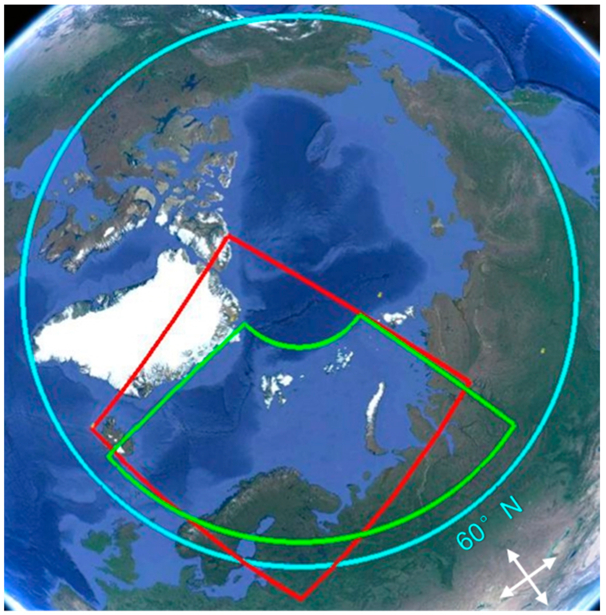
• The COSMO-CLM configuration of the COSMO model: version 5.06; grid spacing 6.6 km; 40 vertical levels; computational domain (countered at the Figure 2 by the red) includes the Greenland, Norwegian, and Barents seas and parts of the Greenland, Kola Peninsula, Kara Sea, and North Pole area. Further in the text, we will refer to it as “COSMO-CLM-A6.6”.
• The configuration of the ICON model for a limited area: grid spacing 6.5 km; 65 vertical levels; domain (countered at the Figure 2 by the blue) covers the circle around the North Pole to 60° N and includes all Arctic ocean seas, Greenland, and the Arctic coasts of the continents. Further in this text, we will refer to it as “ICON-A6.5”.
• The configuration of the ICON model for a limited area (nested into ICON-A6.5): grid spacing 2.0 km, 65 vertical levels, domain (countered at Figure 2 by the green) covers part of the domain ICON-A6.5 close to the Europe. Further in this text, we will refer to it as “ICON-A2”.

The initial data and boundary conditions for COSMO-CLM-A6.6 and ICON-A6.5 were obtained from the ICON global modelling system of the German weather service (DWD). Data that were important for the forecasting of the polar low parameters, such as SST and ice height, were incorporated to the ICON model at the stage of data assimilation [36]. The initial data and boundary conditions for ICON-A2 were obtained from ICON-A6.5. The output data were recorded hourly.

At first glance, the differences in the number of vertical levels in ICON and COSMO seem to be significant (40 versus 65). The density of the vertical levels in the lower atmosphere at which we estimate the main meteorological parameters is important. Here, their density does not vary considerably. For example, up to 1000 m, COSMO has 11 vertical levels and ICON has 10. In the lower 500 m, COSMO has 8 levels and ICON has 7. After 2500 m, the frequency of the levels in ICON and COSMO is equalized. Above 2500 m, their number in ICON grows.

The most important challenges in polar low forecasting involve interactions with the sea surface and the presence and concentration of sea ice. In [29], using the COSMO model with the example of one PL case, it was shown that with a decrease in ice concentration the PL strengthens, and a complete release of the sea surface from ice strengthens and changes the trajectory; it was also shown that one of the factors influencing the evolution of a polar cyclone is the presence of a jet flow with a jet axis at a height of 300 hPa. When the jet flow is weakened and absent in numerical experiments, the cyclone is weakened and changes its trajectory. In [37], it was shown that an increase in the local maxima of the ocean surface temperature field contributes to the intensification of the polar low, and its weakening leads to a smoothing of the baric field and unreliable changes in the trajectories of polar cyclones.

In the model configurations used in this research (COSMO-CLM and in ICON), the surface water temperature does not vary over one day; when the day changes, it changes insignificantly (by a few tenths of a degree or less). Models start with the same temperature of sea water; thus, this factor should not influence the differences in the forecasts between the two models, but could affect the quality of the PL evolution forecast. Neither of the models use data assimilation.

The assessment provided in [38] concluded that the wind speed and wind directions simulated by the ICON model are better than those simulated by the COSMO model. In particular, the RMSEs (root mean squared errors) for these variables decrease when moving from COSMO to ICON. This is to be expected in the forecasting of wind speed when we simulate polar lows.

2.3. Experiments

Model runs were performed for the 7 periods of detected (Figure 1) PLs. All the named PLs were predicted by the models.

Three PLs with a higher wind speed, lower pressure, and longer lifetime were examined in more detail for the periods 26–27 November 2019; 26 February 2020; and 20 March 2020. For each case, model runs using all configurations were performed with a lead time of 48 h. We have started our simulations at 00 UTC every day and a day before when PL was detected at satellite image.

We tried to move forward in the following issues concerning the reliability of using modelling results for the further study of arctic weather, PL dynamics, the formation of high-resolution regional reanalysis datasets, and the development of high-resolution ensemble prediction systems:

• What were the differences between the results of the two modeling systems for CLM community used here based on the COSMO or ICON models? How does the accuracy of PL modelling in both systems decrease with an increasing lead time?
• What is the modelling accuracy of PL?
• What is the sensitivity resolution of the modelled PL? Is there a particular feature in convection permitting higher-resolution models?

The experiments in the framework of the two first named issues were conducted with both models based on COSMO and ICON configurations with similar spatial resolutions. Corresponding numerical experiments aimed to reveal the differences in the modelled features of the PLs between the COSMO and ICON models in the context of migration from COSMO-CLM to ICON-CLM.

The investigations of the third one (based on a comparison of configurations with mesh sizes of 6.6 and 2 km) were based only on ICON simulations with different grid spacings because the ICON simulations showed slightly better results than the COSMO-CLM simulations in the first stage of our investigations and because of the absence of such a test before, while such research is necessary due to the upcoming migration to ICON-CLM.

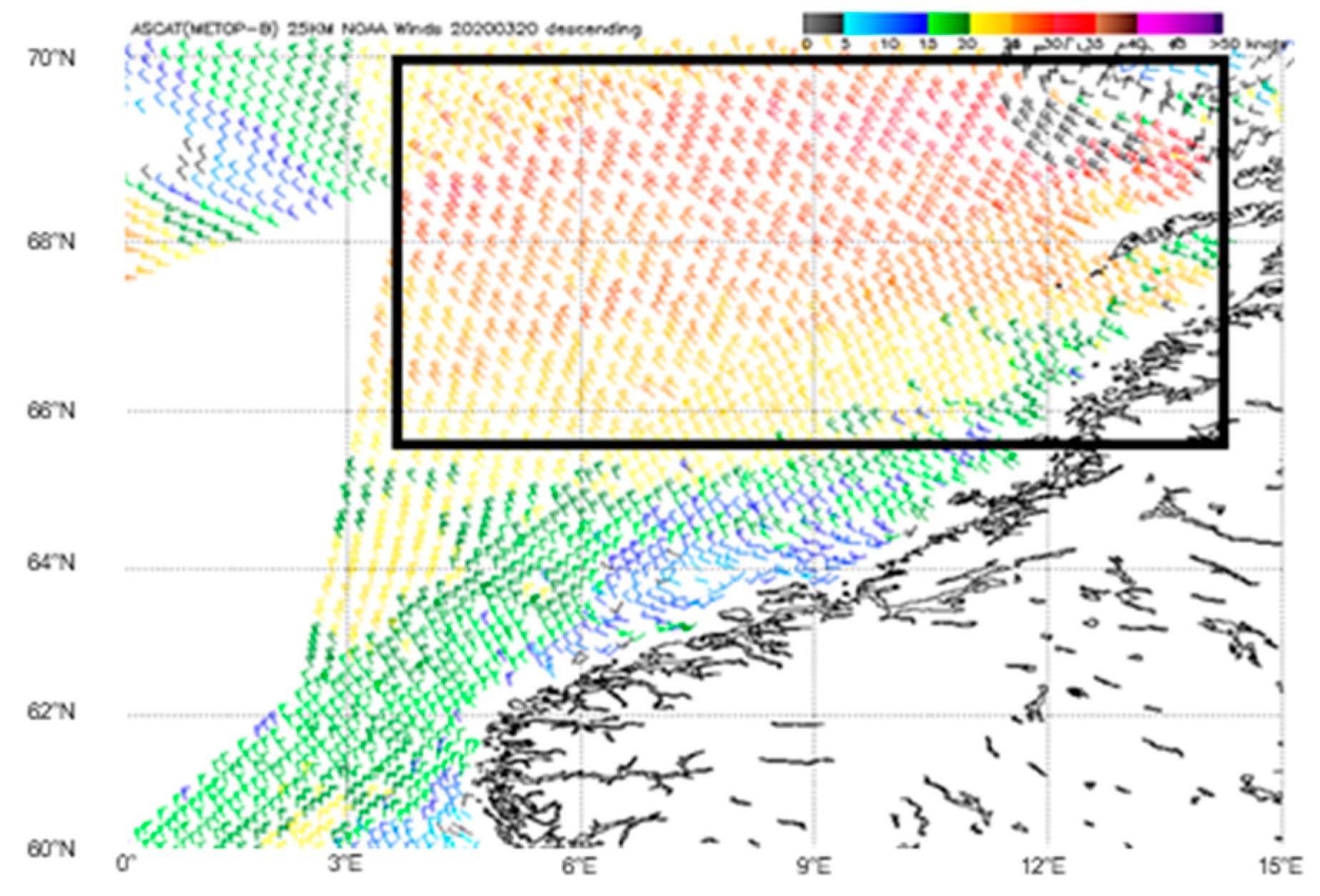
2.4. Verification Data

Satellite images were used for the identification of a PL’s location during its lifetime and the configuration of cloud patterns within the cyclone. This was supported by an ERA5 reanalysis (grid spacing about of 30 km) and the ASCAT scatterometer data (resolution about of 25 km) for the detection of the actual wind speed in comparison with the modelled results. However, the named resolution is not sufficient to give the detailed picture of the wind speed (more or less reliable) and gusts (seem to be underestimated) in the wind field of a cyclone with a horizontal scale of several hundred kilometers.

Data for synoptic stations located onshore and on islands were used for quantitative assessments. However, we must keep in mind that the net of such stations is rather sparse, which makes the problem of interpolation critical, at least for spatial scales of PLs.

3. Results

3.1. Comparison of PL Modellling Skill based on COSMO-CLM and ICON

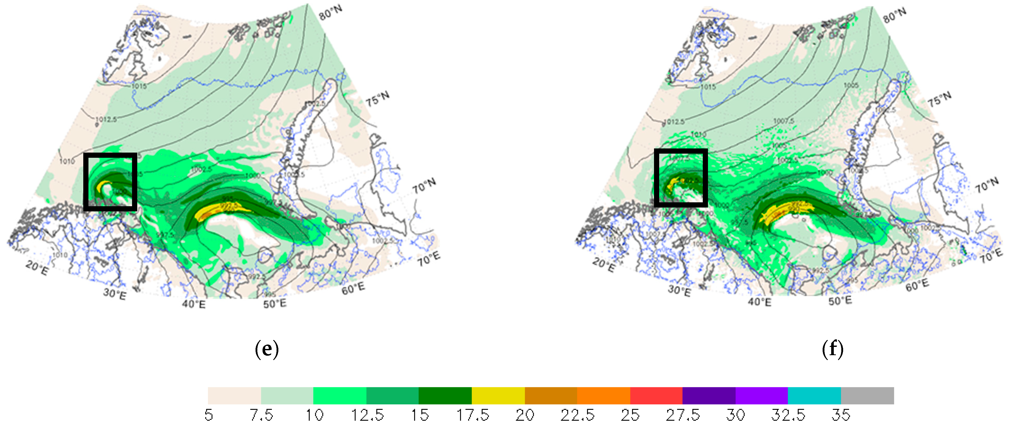
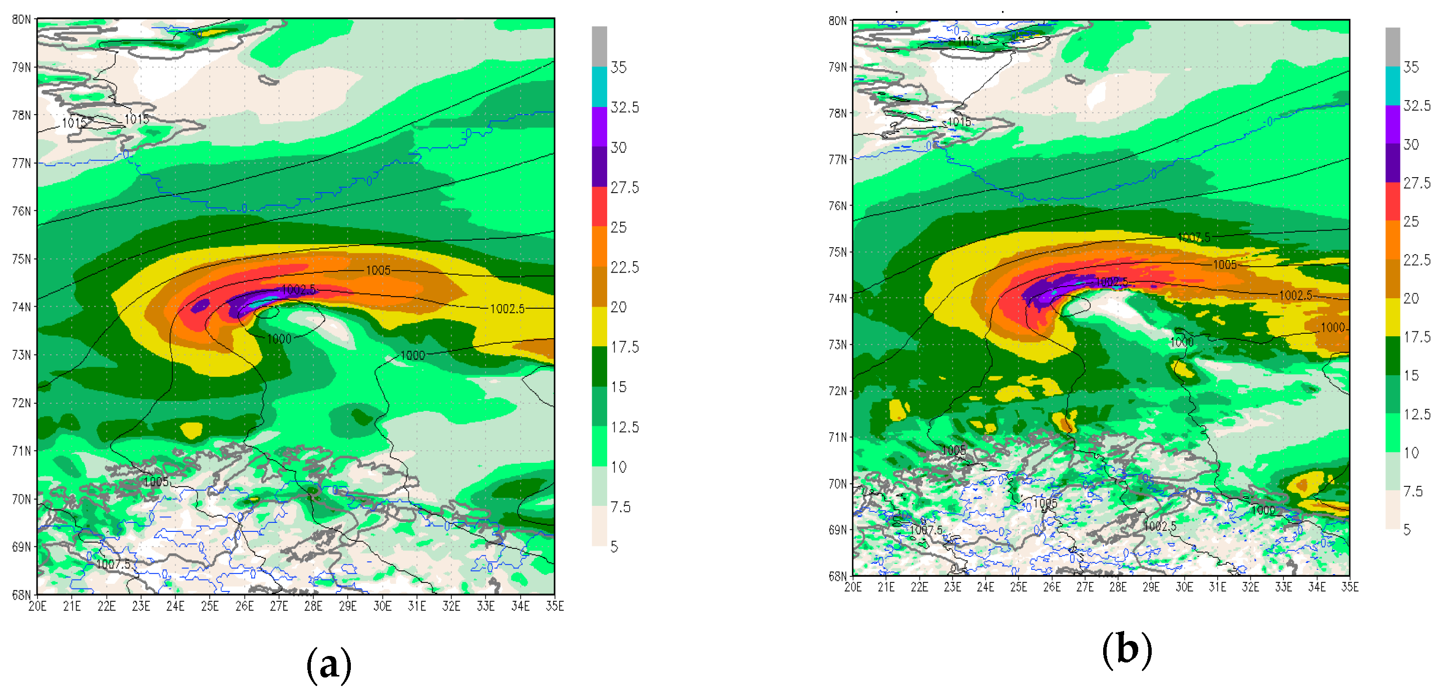
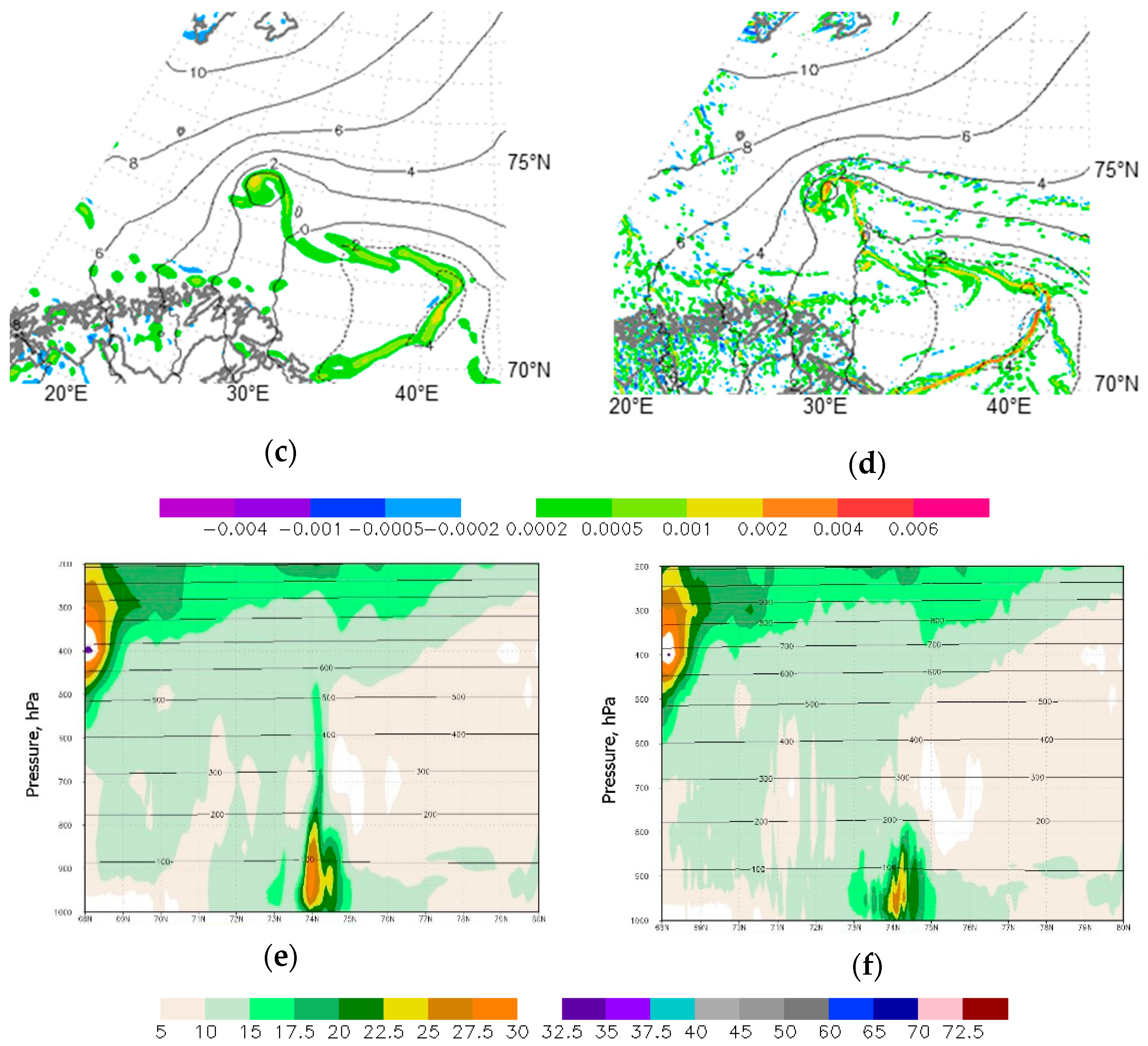
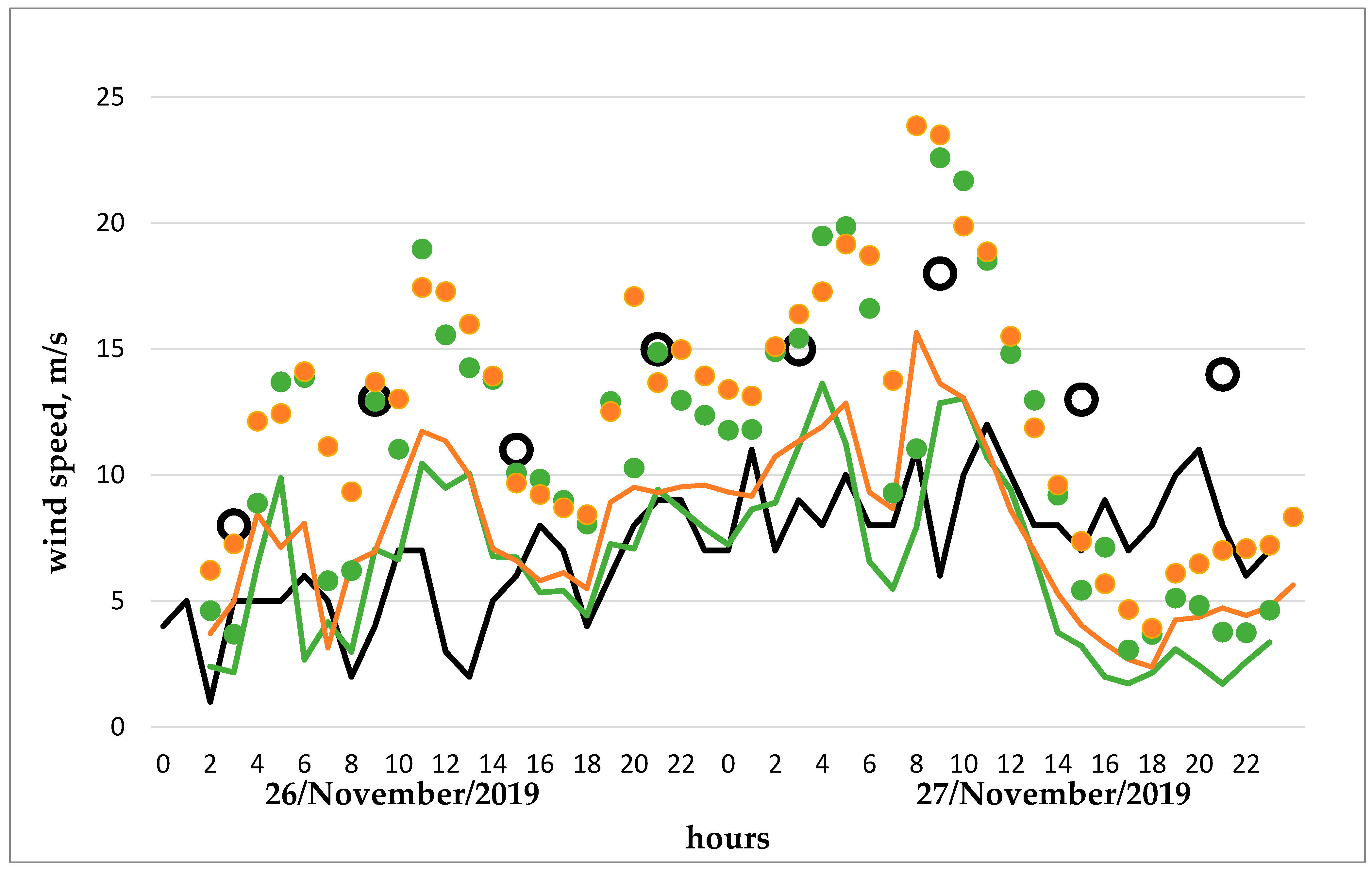
3.1.1. Case of PL of 26–27 November 2019

The PL of 26–27 November 2019, is one of the most intensive for the studied cold period of 2019–2020. It occurred on 26 November 2019, southeast of Svalbard and moved to the south, reaching the Norwegian coast at night on 27 November and weakened (Figure 3). An initial assessment of the models’ prediction quality for the cyclones was conducted on the basis of the analysis of the wind field and sea-surface pressure. Forecasts with lead times of 12 and 36 h were produced for each case. In each case, the forecasts with a lesser lead time were the most successful. Later, we will compare the ICON and COSMO-CLM in the forecasting of PLs with lead times of less than 24 h.

Figure 4 shows the wind speed at 10 m and wind gust simulations from the initial data at 00:00 UTC, 26 November, with a lead time of 18 h (valid time 18:00 UTC, November 26). Satellite images of this polar low are shown in Figure 3.

In Figure 4b,d, in comparison with the satellite images (Figure 3) and scatterometer data (Figure A1), we see the simulation of close scenarios of PL development by COSMO-CLM-A6.6 and ICON-A6.5. However, we can suppose that the ICON predicted the minimum of sea-level pressure at the center of PL and the cyclonic movements a little better than the COSMO-CLM did. It is likely that he closed contours of pressure lines better correspond to the transition from the comma to the spiral structure phase of this PL (Figure 5b). According to the ICON results, the wind speed at the center of the PL reached 17.5–20 m/s, the ones from COSMO-CLM were in the interval of 15–17.5 m/s, and the scatterometer data were in the interval of 35–40 knots (approximately 18–21 m/s) (Figure A1).

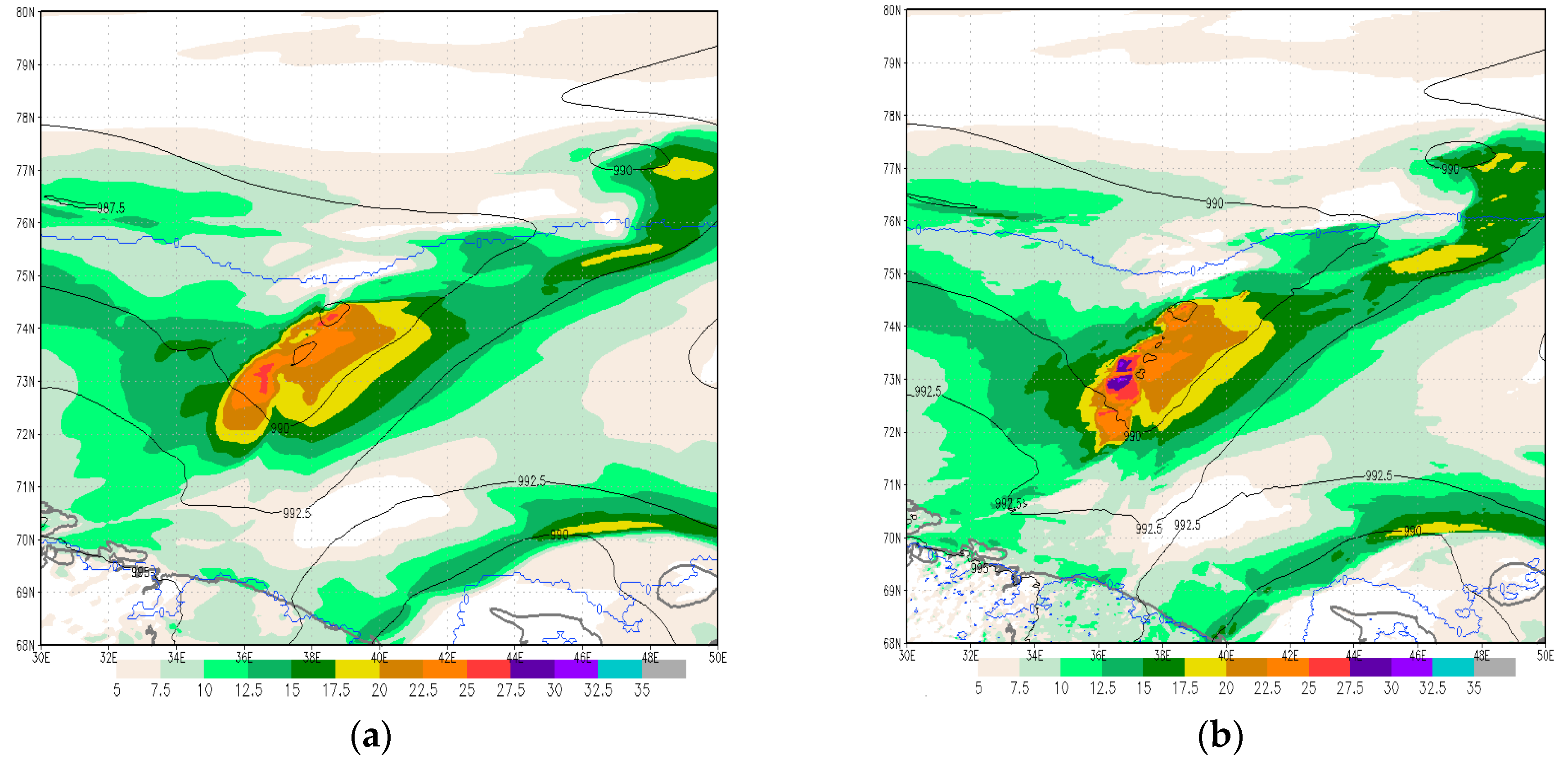
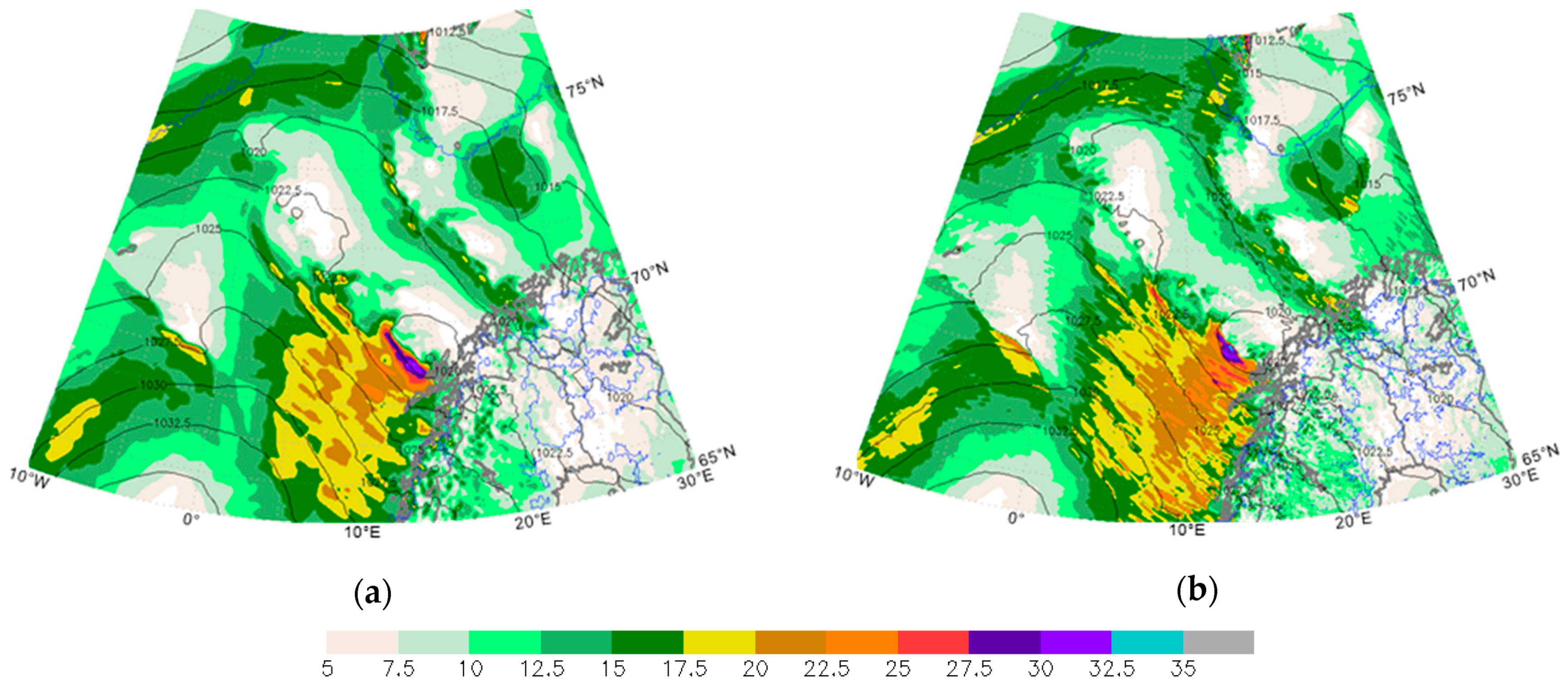
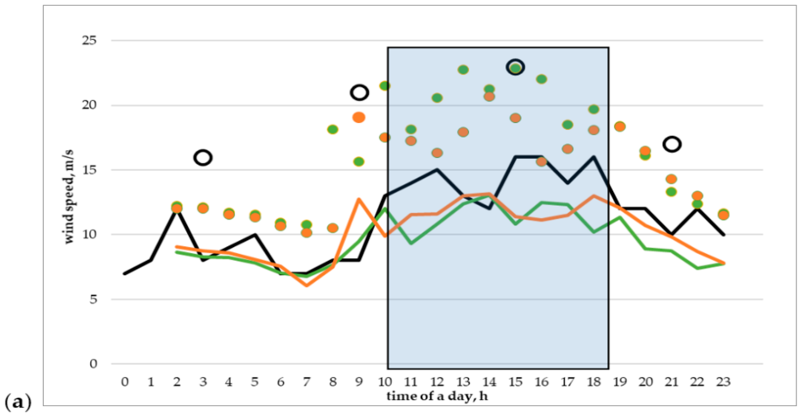
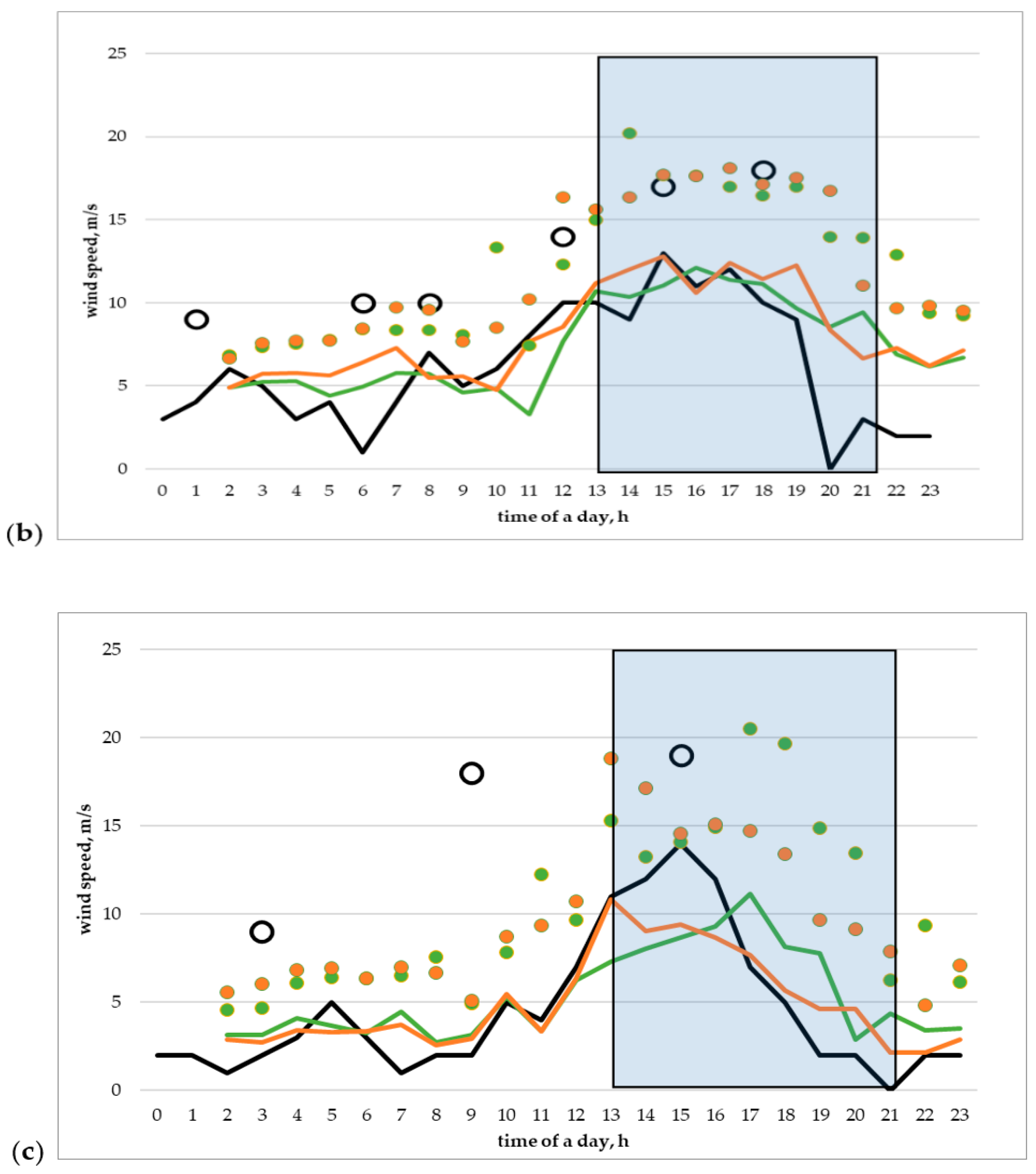
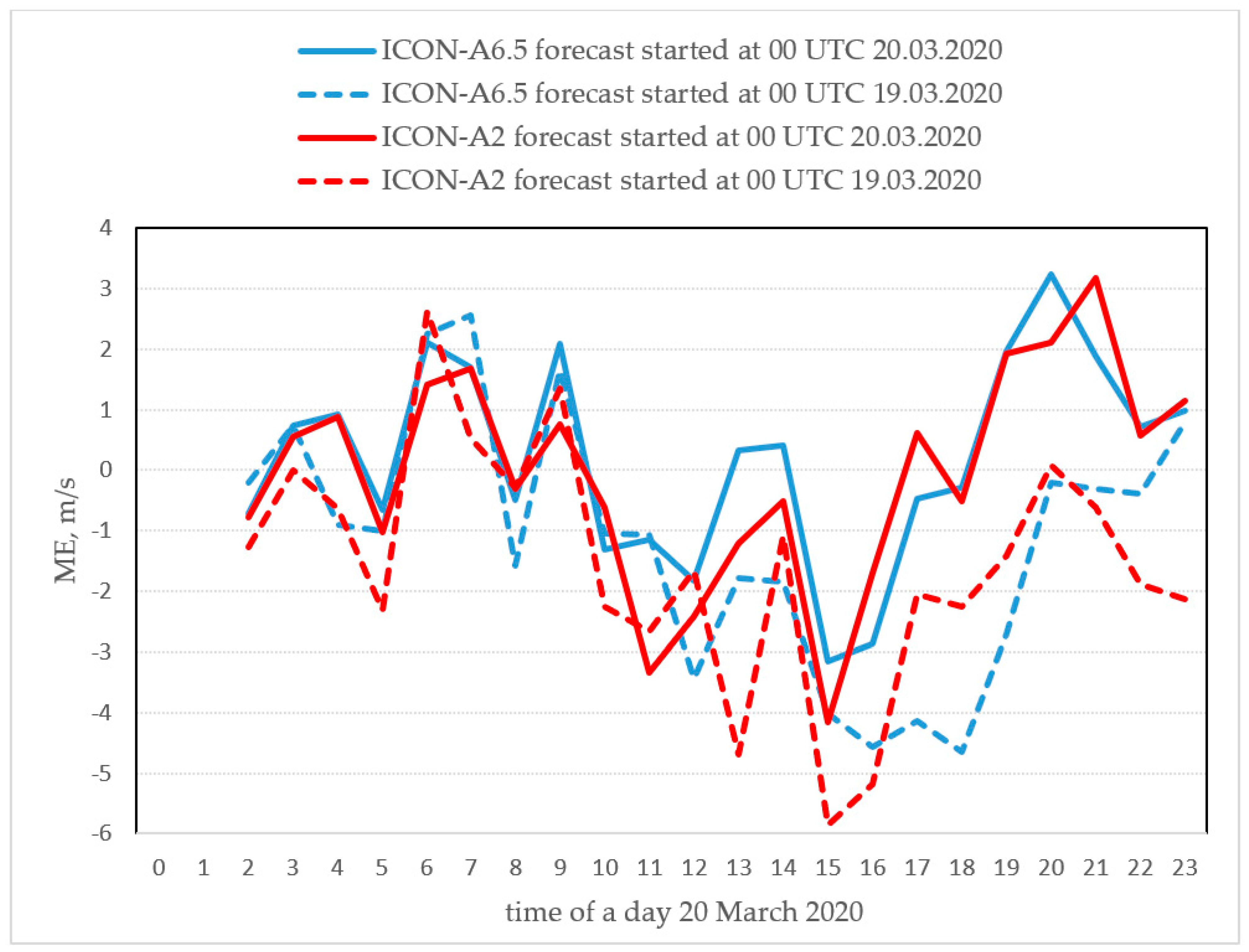
3.1.2. Case of PL of 20 March 2020

The polar low observed near the Norwegian coast on 20 March 2020, was formed during the day of 19 March in the west of the Norwegian Sea in the cold air flows from the sea ice near the eastern part of Greenland. Then, the vortex moved generally to the east with a steering flow along approximately 70° N, activating during the movement. Following the PL trajectory in the satellite images allows us to conclude that at 13:00 UTC on March 19, the PL with a comma cloud structure can be observed in the Jan Mayen island region (Figure 5a).

The PL approached the Norwegian coast on 20 March 2020; as the previous case, it was better reproduced in terms of average wind, wind gusts, and atmospheric pressure in the ICON simulation.

The sensitivity of the modelling accuracy to increases in the forecast lead-time in this case has been studied on the basis of numerical experiments with different base times and lead times for the same valid time. The results can be seen in Figure 6; with a lead time of 36 h, both models (started 1 day before) produced approximately the same values for wind gusts, but with different locations of the PL (Figure 6c,d) and more intense PL destruction near Scandinavian coast (for COSMO-CLM, which was additionally quicker) for a lead time of 12 h than were seen in reality.

With a lead time of 36 h, the PL according to COSMO-CLM was significantly displaced to the northwest (Figure 6c); in the case of ICON, the zone of strong winds was close to that obtained in the experiment with a short lead time (Figure 6a), however the cyclonic vortex itself was reproduced worse (Figure 6d). For a 12-h lead time, the PL approached the coastline, which can be seen in the satellite images and verified by the forecasts with a 12-h lead time (Figure 5, Figure 6a,b).

3.1.3. Case of PL of 24–27 February 2020

Identical to the two previous cases analyzed above, results were obtained for the PL of February 24–27. In the ICON-A6.5 simulations, the wind speed also exceeded the wind speed predicted by COSMO-CLM-A6.6 and the wind gusts were 7.5 m/s higher. The simulation results of the sea-level pressure were practically identical (Figure A2) for both experiments with a lead time not exceeding 24 h.

Based on all the experiments, we have seen that the modelling skill (PL localization, pressure minimums etc.) falls significantly with an increase in the forecast period to more than 1 day.

An initial assessment based mainly on the comparison of model data with satellite images of polar lows in the COSMO-CLM-A6.6 and ICON-A6.5 results (both with grid step about 6.6 km) demonstrated that, in all the analyzed cases, both the models showed close results and are able to produce polar lows for the first modelling day. However, in all the distinguished cases the ICON forecasts were a little more accurate; the forecasts of the sea-surface pressure, the location of the PLs, and the wind gusts were better than the forecasts produced by COSMO-CLM. The main features of most of the COSMO-CLM-A6.6 simulations are an underestimation of the wind speed and a decrease in the cyclone depth, as well as a faster decline in the forecast accuracy with an increase in the lead time. Some of these conclusions made based on ICON-AR6.5 comparisons with observations showed in the Section 3.2.

The second stage of this work is devoted to an analysis of the forecast quality of the same cases with an ICON model with resolutions of 2 and 6.5 km and a study of the structure and peculiarities of the PLs produced by the model, as well as a point data verification using the observation data of wind speed.

3.2. Modelling of PLs with Increasing Model Resolution

For the selected PLs, numerical experiments were carried out using two configurations of the ICON model (see Section 2.2): ICON-A6.5 and ICON-A2. Hereafter, we will assess again the same three cases of PLs with a more detailed analysis but simulate them with an ICON model configuration with different grid spacings of about 6.6 km and 2 km.

3.2.1. Case of Polar Low of 26–27 November 2019

Figure 7 shows the 10 m wind speed and sea-level pressure forecasts of 4-, 19-, and 29-h lead times from a base time of 00:00 UTC 26 November 2019, according to two configurations: ICON-A6.5 and ICON-A2. Both configurations predict the occurrence of polar lows in approximately the same way; the maps show that, at 4:00 UTC at the edge of the sea ice southeast of Svalbard, a minimum atmospheric pressure and a zone of increased wind speed (from 12.5 to 15 m/s) are formed.

The differences in air temperatures between the sea surface temperature and the temperature at 500 hPa (exceeding the threshold 41.4 K) and 700 hPa (threshold 22.8 K) are the criteria for identifying the possibility of PL initiation [7]. Both of these criteria are satisfied in the area of polar low occurrence (Figure A3). The area in which the second criterion (T_sea-T₇₀₀) is satisfied is much more extensive than the area of the first criterion (T_sea-T₅₀₀) (see Figure A3). Additionally, it can be seen that the area of the criterion for (T_sea-T₅₀₀) corresponds to the full lifetime of this PL.

According to the simulations, the wind speed in the PL ranges from 20 to 22.5 m/s at 19:00 UTC, 26 November, while the PL deepens (Figure 7c,d). It is noteworthy that a synoptic-scale cyclone can be seen to the east of the polar low in the Barents Sea, which is confirmed by the satellite imagery (Figure 3c). This then shifts to the south of Novaya Zemlya. At 00:00 UTC, 27 November, the wind speed in both cyclones ranges from 17.5 to 22.5 m/s. By 05:00 on 27 November 2019, the PL approaches the coast of the Scandinavia, where the wind speed decreases, and the atmospheric pressure rises (Figure 7e,f).

According to the ASCAT data [33], the surface wind speeds reached 15–17.5 m/s at 18:00 on 26 November (in the ASCAT data, 35 knots corresponds to 18 m/s), while, according to the model, they ranged from 17.5 to 22.5 m/s. Most likely, this indicates that the higher resolution of the model (6.5 and 2 km) compared to the ERA5 reanalysis and the ASCAT scatterometer (the resolution of which is 25 km) allows obtaining a more detailed wind field near the center of the polar low. The data of ERA5 and ASCAT can be found in Figure A1.

The results of more detailed analysis of the modelling are shown in Figure 8. The polar low and the synoptic-scale cyclone located to the east are quite well expressed in the vorticity field; however, the PL is shown in more detail by ICON-A2, and its absolute values are higher than in the ICON-A6.5 results. It is remarkable that, in the ICON-A6.5 simulations, the PL is deeper and wind speed inside it at about 950 hPa is stronger, but at the near-surface level the 10 m wind speed and gusts have close values to those of our simulations with different grid steps.

As mentioned above, this PL began to decay at night on 27 November, when it came to the coast of Norway. The presence of operating coastal meteorological stations in the vicinity of the polar low landfall allows us to carry out a point forecast verification of the wind speed and wind gusts. The Norwegian station Honningsvåg airport, located in a small bay in the north of the country, was selected to compare the forecasts with observations.

Figure 9 shows the wind speed and gusts in Honningsvåg on 26 and 27 November based on the observational and forecast data. The averaged data of the nearest model grid point and four neighboring ones were used here as prognostic data. Three of these grid points were located in the sea and two of them on the land (one of them is more than 1 km away from the coastline). In Figure 9, the rectangle shows the time period when the polar low affected the station. Wind gusts at the station are presented in the available datasets only for 6-h intervals (shown in the picture for the middle period). We averaged the forecasts in the model grid point closest to the station and four neighboring ones in order to obtain more representative forecast data and compare them with the observational data conveniently. We compared the model data at four grid points around the station before the procedure of averaging; this showed that the data are almost identical (the spread between the values of the gusts at different nodes in most cases ranged from 2 to 2.5 m/s, but sometimes reached 5 m/s; at the same time, the spread of wind speed at 10 m was insignificant). The wind gusts ranged from 15 to 18 m/s during the passage of the polar low. Both model configurations predicted the values of wind gusts quite accurately for 26 November 2019 and worse for 27 November 2019 (with a lead time of more than 24 h).

The wind speed is predicted with larger errors for this period, which may be associated with its strong variability due to the orographic conditions of meteorological stations. Observation station Honningsvåg (71°01’ N, 25°59’ E) is located at the coastal line in a bay surrounded by small hills and islands. The values for the 10 m wind speed and gusts are shown in Figure 9 with green and orange curves and points. For most of the day on 26 November and the morning of 27 November, the simulated 10 m winds were overestimated (see ICON-A6.5). For example, the wind speed was predicted to be equal to 16 m/s at 08:00 UTC on 27 November, while in reality it did not exceed 11 m/s. After 13–14 h on 27 November, the differences between the observations and the model increase. According to the observations, the wind in the Honninsvåg area was 5–10 m/s with gusts up to 15 m/s, but according to both models, it was below 5 m/s, and no significant wind gusts were observed. This may be due to two factors: first, by this time the lead time of the forecast was 37 h or more, which itself can affect the quality. Secondly, after 15 UTC the wind changed direction from north-east to the east. It is likely that due to the peculiarities of the model orography and coastline in the Honninsvåg region, a change in wind direction could affect its speed, as it encountered an orographic obstacle.

3.2.2. Case of the Polar Low of 24–26 February 2020

The polar low that occurred over the Barents Sea on 26 February formed in the cold northern air stream from Svalbard in the afternoon of 24 February to the south and then to the east, developing as it moved; we tracked the vortex trajectory according to satellite images (Figure 10). This is the longest-lived PL we have identified during the studied cold period.

Figure 11 shows the vertical profiles of the wind speed modulus according to the model data. It can be seen that the maximum wind speed in the PL circulation (approximately near 925 hPa) corresponds to a high wind speed of 500 hPa (map of H500 is shown in Figure A4). In the case of modelling with a coarser resolution, both maxima are joined, and for higher-resolution modelling this relation is more complicated. As for the case of the PL of 26–27 November (Figure 7), the wind speed maximum is located near the level of 925 hPa, and the area of wind values exceeding 20 m/s in ICON-A6.5 is more extended than in the case of ICON-A2. The interaction with the H500 flow should be explored in future investigations. It is evident that the atypical tracking of this PL was due to its interaction with the middle troposphere dynamics.

Despite the fact that the PL according to the satellite images originated on 24 February (Figure 10a), it appeared on both the ICON configuration maps of forecast only on the night of 26 February as a low-pressure area with strong winds (by definition, the wind speed near the surface in a polar low should not be less than 15 m/s). Model simulation from 00 UTC 25 February shown a zone with an increased wind speed (up to 15 m/s) and was identified in the Barents Sea, but it was rather vague and shifted to the northeast a little faster than the real PL. In this case, the model was able to predict a polar low when a cyclonic disturbance was already present in the initial conditions. Qualitatively, both the model configurations predicted the region of increased wind speed and low atmospheric pressure identically; however, the ICON-A2 predicted a stronger maximal value of wind gusts (up to 27.5 m/s at 03:00 UTC) than the ICON-A6.5 did (up to 25 m/s at 03:00 UTC). Even stronger differences in wind gusts were observed at 05:00 UTC, with ICON-A2 showing them up to 32.5 m/s and ICON-A6.5 showing them up to 27.5 m/s (Figure 12a,b). Probably these differences occurred because of the fact that increased grid step allows to simulate horizontal motion in more details. However, we cannot check which were real wind speeds and gusts because of the absence of the appropriate observations above the sea.

The zone of strongest winds in the polar low is accompanied by an increased vorticity in this area (Figure 13a,b), while it is noteworthy that the maximum vorticity values are located near the land surface but not at the level of 500 hPa, where stronger wind speeds were observed. The zone of positive vorticity values is adjacent to the zone of negative values on the profiles along 73° N and 38.5° E, which is also one of the criteria for identifying polar lows.

3.2.3. Case of PL of 19–20.03.2020

Figure 14 shows the forecast of wind gusts produced by two model configurations. It can be seen that while the wind speeds only in some regions exceed 17.5 m/s, the wind gusts reached 32.5 m/s, which is considered to be a dangerous value in terms of synoptic classification. The formed comma cloud structure was formed on the evening of March 19 (Figure 5), but the wind speed did not exceed 15 m/s (gusts reached 22.5 m/s). By the morning of 20 March, the wind speed exceeded 17.5 m/s and the wind gusts reached 32.5 m/s (Figure 14).

The forecasts starting at 00:00 UTC on 19 March did not reproduce the atmospheric pressure minimum and an increase in the wind speed to 17 m/s. However, in the forecast starting at 00:00 UTC on 20 March, the minimum of atmospheric pressure and the area with a wind speed exceeding 17.5 m/s were successfully predicted. Nevertheless, with the forecast of 19 March, the PL was reproduced in the model, just its intensity was lower (Figure A5).

Figure 15 presents the satellite data for the 10 m wind speed obtained from ASCAT for 11:00 UTC, 20 March. It shows that the polar low reached a large size near the Norwegian shoreline and the 10 m wind reached 35 knots, corresponding to 18 m/s. These values should be compared not with the gusts presented in Figure 14, but with the wind speed shown in Figure A5. As shown in the forecast of ICON-A6.5 for valid time 12:00 UTC, the wind speed ranges from 17.5 to 20 m/s. To the south of the polar low center, the wind speed does not exceed 12.5–17.5 m/s. These values correspond well with the ASCAT data.

A noticeable increase in the 10 m wind speed and gusts was observed at some coastal and island meteorological stations when the PL approached the coast of Norway. The simulations and a comparison with the data of coastal observations are shown in Figure 16 (the rectangle shows the time period in which the PLs influenced the coastal wind speed). We have to understand that the location of the northern Norwegian observation stations is partially closed to the wind by chains of islands, rocks, and hills. It is important to note that Skrova Lighthouse station is the only station on an open surface. The observations at other stations are strongly dependent on orographic features.

Following Figure 16, it can be seen that the ICON-A2 and ICON-A6.5 are close in their forecasts. The values of wind gusts were reproduced with accuracy; in most cases, both model configurations also captured the maximum wind speed in the period from 14 to 17 UTC quite successfully. However, the weakening wind on the evening of 20 March was overestimated by the both ICON configurations for Skrova lighthouse and Stokmarknes airport.

We also evaluated the dependence of the wind speed forecast on the lead time. The mean error (ME) of three stations (Röst, Skrova, Stokmarknes) is presented in Figure 17. It can be seen that the mean errors are very close between the two model runs in the time before the PL came to the coastal line (around 12 UTC); after that time, the ME of the forecast starting at 00 UTC 19 March 2020 (with a bigger lead time) began to be higher than the forecast starting at 00 UTC 20 March 2020 (with a smaller lead time). From this, we can conclude that, in this case, the largest forecast errors with a greater lead time are observed at the moment the cyclone reaches the land, and in this moment wind speed is underestimated. Figure 17 shows the ME of two model configurations—Arctic-A6.5 and Arctic-A2. It is noticeable that, during first half of the day, the ME are close between the two model configurations. The main differences are found in the forecasts with a larger lead time at the moment when the PL was already on land. In this case, the model with a grid step of 2 km has a large error in absolute value, while the model with a grid step of 6.5 km has a large error for a longer time. The mean RMSE and RMSE for different stations during the cases when PL reached the coast can be found in the

Table 1. RMSE of the ICON-A6.5 and ICON-A2 forecasts of 10 m wind speed.

Stations	Lead Time 24 h, Forecast Started at 00 UTC 20.03.2020		Lead Time 48 h, Forecast Started at 00 UTC 19.03.2020
	Arctic-A2	Arctic-A6.5	Arctic-A2	Arctic-A6.5
	RMSE	RMSE	RMSE	RMSE
Röst, 20 March 2020	2.09	2.02	2.36	1.92
Scrova, 20 March 2020	2.16	2.17	2.15	2.26
Stokmarknes, 20 March 2020	2.13	1.70	2.03	2.50
Honningsvåg, 26 November 2019	2.09	2.30	2.51	2.53
Mean RMSE	2.12	2.05	2.26	2.30

. The smallest RMSE with a lead time of 24 h was obtained when Arctic-A6.5 was used. Arctic-A2 shows a better forecast with a larger lead time.

Figure 18 shows the cross-section along 69.5° N. Figure 18 gives us an impression that both the model configurations simulated the PL as independent circulation system, without explicit interaction with the powerful jet stream located at heights. As for the other PL cases analyzed, ICON-A2 simulates a smaller area of strong winds inside PL and makes its structure more detailed. Both versions of the model predicted comparable heights of the PL: in the most active stage, it reached heights of 800 hPa. The small dimension of PL strengthens the complexity and importance of its numerical prediction.

4. Discussion

A comparison of different configurations of the models and their initial verification were carried out using three types of data: data from the ERA5 reanalysis with a resolution of 30 km [39], data on wind speed obtained using the ASCAT scatterometer (with a resolution of 25 km), and conventional data of synoptic stations. These are all the available data on wind speed and gusts for the investigated period. The interpretation of the comparison results shown in this study should be made taking into account some peculiarities in the data used.

The ERA5 reanalysis cannot be used itself as a reliable source for model verification since it is a modelling product and has a rather coarse resolution. The ASCAT scatterometer has a resolution 2–6 times coarser than the grid spacing of the used configurations; nevertheless, it is a fairly reliable source for determining the wind speeds over the sea [40].

A point-to-point verification of the model results with observation data at coastal and island meteorological stations also has advantages and disadvantages. Among the advantages is the certainty of the direct measurement data. Among the disadvantages, we have to take account that the local geographical features (variable orography and coastline) of the stations of the Northern Norwegian coastline have a strong influence on the wind fields.

We cannot request our model configurations to describe accurately the wind inside sub-grid hills and small islands. The upscaling ensemble approaches may be effective for the interpretation of modelling results near the Norwegian coastline. It seems reasonable to assimilate ship and aviation observations for the assessment of polar low parameters.

5. Conclusions

A number of cases of PL formation in the cold period of 2019/2020 were identified over the Barents and Norwegian seas using satellite images. A map of their trajectories has been built and numerical experiments using the COSMO-CLM and ICON models with a grid spacing about of 6.6 km were carried out in the first stage of this work.

For the detected periods, the numerical experiments were performed with configurations of COSMO-CLM and ICON models with grid spacings of 6.6 and 2 km. All the cases of detected PL were successfully simulated by all configurations. The experiment results showed the possibility of the COSMO-CLM and both ICON configurations to accurately predict the PL development and tracking. However, a rapid decrease in the accuracy of the modelling results was detected after the first 24 h of modelling time for all configurations. We can suppose that including in the simulations changes during the runs of sea surface temperature [28] as well as data assimilation could be useful, since the initial data in our experiments were presented with 13 km grid spacing.

The comparison of the simulations based on the COSMO-CLM and ICON models with the same grid spacing of about 6.6 km (surface pressure, location of the PLs, the wind speed and gusts) showed a slight advantage of the ICON-based configuration. The loss of quality after the 24 h lead time was quicker from the COSMO-CLM. In [28] it is shown that the COSMO model reproduced the origin and trajectory of a PL with a 6-h lead time. In the experiment, with a lead time of 18 h, the model COSMO reproduced the origin of the PL, but was significantly mistaken with its trajectory. It was shown in [33] that using more accurate information on the ocean surface temperature and its timely (every 3 h) update allow the COSMO model to simulate a PL with a 48-h lead time. In our experiments, the water temperature was updated once a day, and the analysis of individual cases showed that the ICON model simulated a PL in 18–24 h without updating the ocean temperature, this support previous conclusion about quicker loss of quality of the COSMO-CLM model with increasing the lead time. In some ICON simulations of PL cases (for example, on 24–26 February) a polar low appears in The Barents Sea only after updating the initial data and with a 6-h lead time. From that we can conclude that the success of the forecast in each specific case depends not only on the configuration of the model, but also on the features of the polar low itself. It will be interesting to pay more attention to this in the next studies.

A comparative analysis of the modelling results from the ICON models with grid spacings of 2 and 6.6 km was carried out. The atmospheric pressure, wind speed, wind gusts near the surface and at altitude, vorticity field, profiles of the vertical speed, and temperature were verified for each of the studied cases of PLs. The forecast fields of meteorological values were compared with the ERA5 reanalysis data. The wind data were also compared with the data obtained using the ASCAT scatterometer and with the observational data delivered from meteorological stations.

The numerical experiments did not demonstrate principal differences between the modelling results of the model configurations based on the ICON models with grid spacings of 6.6 and 2.2 km, comparable with observational uncertainty. We can note that the difference between the ICON and COSMO simulations with the same resolution was closer than that between two configurations of ICON with different grid spacings. However, some results showed that the ICON configuration with a grid spacing of 2 km was a little more accurate than the one with 6.6 km. It was shown that, in most cases, the ICON model with a 2 km grid spacing predicts stronger wind, which was confirmed by measurements. On the other hand, there were several cases where a 6.6 km ICON forecast with a stronger wind was overestimated. The smallest RMSE with a lead time 24 h were obtained when Arctic-A6.5 was used. Arctic-A2 shows better forecast with a larger lead time. However, it should be noted that the difference in the resulting average RMSE is insignificant. It is very likely that the orographic features of the surface and wind direction can strongly influence the wind speed in the polar low and its forecast when it comes to the land.

It is shown that the main properties of polar lows (vertical motion, vorticity) are represented by both model configurations, but 2 km grid steps reproduce the PL structure in more detail with smaller strong wind domains and a more complicated structure. In general, the advantages of the 2 km version of the model are not always obvious. In particular, simulations with ICON-A2 provide more detailed map of wind speed, wind gust, and vorticity, areas with high wind speed became more compact and more intense in comparison with ICON-A6.5 simulations. But point-to-point verification by observations at coastal and island stations did no show significant advantages of ICON-A2 in comparison with ICON-A6.5. In [33] the influence of the transition from a grid step of 6.6 km to 2.2 km had been assessed, and authors concluded that a decrease in grid step had a much smaller effect than a change in the ocean surface temperature and sea ice boundaries. We examined dependence on the model grid steps in more details than it was done in [33] and our conclusion consistent with previous study. Nevertheless, we think that in order to find an optimal configuration of the ICON model for PL forecasting, a more detailed study of the dependence of the simulation quality of the PL and its interaction with the coast on the choice of the grid step is required. Thus, the special investigation of modelling with different resolutions of the process of destruction of PL and its interaction with coastlines seems to be interesting for further research.

An analysis of the 3D structure of the simulated PLs was performed. Our experiments confirmed the low altitudes of the developed PLs (maximum to height 800–850 hPa, corresponding to 1–1.5 km) and the very small cross-section sizes (less than 200 km) of the wind modified domains in comparison to the jet streams of the middle atmosphere (global frontal zone) situated nearby. Our experiments confirmed that PLs have the strong maximum of absolute vorticity inside the extended area, including the jet stream domains. Experiments have shown that, in some cases, PLs can interact with global frontal flows of the middle troposphere in terms of kinetic energy exchange. A more detailed investigation of these processes based on the ICON-A6.5 and ICON-A2 configurations is planned the next time.

The criteria for the development of the PLs described in the literature were analyzed, and it was shown how they appeared in the simulations for all cyclone cases.

An analysis was carried out of the dependence of the forecast success on its lead time. The results showed that all the considered PL cases were successfully simulated with lead times of 3 to 24 h. The simulations were less successful with lead times of more than a day. A detailed examination of some PLs showed that there were situations when a polar low that appeared in a cloudy field did not demonstrate itself in the wind field for a long time (up to two days).

References

1. Heinemann, G.; Saetra, Ø. Workshop on polar lows. BAMS 2013, 94, ES123–ES126. [Google Scholar] [CrossRef] [Green Version]
2. Rasmussen, E.A.; Turner, J. Polar Lows: Mesoscale Weather Systems in the Polar Regions; Cambridge University Press: Cambridge, UK, 2003. [Google Scholar] [CrossRef] [Green Version]
3. Harold, J.M.; Bigg, G.R.; Turner, J. Mesocyclone Acticity over the North-East Atlantic. Part 1: Vortex distribution and variability. Int. J. Climatol. 1999, 19, 1187–1204. [Google Scholar] [CrossRef]
4. Wilhelmsen, K. Climatological study of gale-producing polar lows near Norway. Tellus A 1985, 37, 451–459. [Google Scholar] [CrossRef]
5. Lutsenko, E.I.; Lagun, V.E. Polar Mesoscale Cyclonic Eddies in the Arctic Atmosphere; Arctic and Antarctic Research Institute: St. Petersburg, Russia, 2010. [Google Scholar]
6. Mokhov, I.I.; Akperov, M.G.; Lagun, V.E.; Lutsenko, E.I. Intense arctic mesocyclones. Izv. Atmos. Ocean. Phys. 2007, 43, 259–265. [Google Scholar] [CrossRef]
7. Smirnova, J.E.; Golubkin, P.A.; Bobylev, L.P.; Zabolotskikh, E.V.; Chapron, B. Polar low climatology over the Nordic and Barents seas based on satellite passive microwave data. Geophys. Res. Lett. 2015, 42, 5603–5609. [Google Scholar] [CrossRef] [Green Version]
8. Stoll, P.; Graversen, R.G.; Noer, G.; Hodges, K. An objective global climatology of polar lows based on reanalysis data. Q. J. R. Meteorol. Soc. 2018, 144, 2099–2117. [Google Scholar] [CrossRef] [Green Version]
9. Terpstra, A.; Michel, C.; Spengler, T. Forward and Reverse Shear Environments during Polar Low Genesis over the Northeast Atlantic. Mon. Weather Rev. 2016, 144, 1341–1354. [Google Scholar] [CrossRef]
10. Gavrikov, A.; Gulev, S.; Markina, M.; Tilinina, N.; Verezemskaya, P.; Barnier, B.; Dufour, B.; Zolina, O.; Zyulyaeva, J.; Krinitskiy, M.; et al. RAS-NAAD: 40-yr High-Resolution North Atlantic Atmospheric Hindcast for Multipurpose Applications (New Dataset for the Regional Mesoscale Studies in the Atmosphere and the Ocean). JAMC 2020, 59, 793–817. [Google Scholar] [CrossRef]
11. Laffineur, T.; Claud, C.; Chaboureau, J.-P.; Noer, G. Polar lows over the Nordic Seas: Improved Representation in ERA-Interim Compared to ERA-40 and the Impact on Downscaled Simulations. Mon. Weather Rev. 2014, 142, 2271–2289. [Google Scholar] [CrossRef]
12. Michel, C.; Terpstra, A.; Spengler, T. Polar Mesoscale Cyclone Climatology for the Nordic Seas Based on ERA-Interim. J. Clim. 2017, 31, 2511–2532. [Google Scholar] [CrossRef]
13. Bromwich, D.H.; Wilson, A.B.; Bai, L.-S.; Moore, G.W.K.; Bauer, P. A comparison of the regional Arctic System Reanalysis and the global ERA-Interim Reanalysis for the Arctic. Q. J. R. Meteorol. Soc. 2016, 142, 644–658. [Google Scholar] [CrossRef] [Green Version]
14. Krinitskiy, M.; Verezemskaya, P.; Grashchenkov, K.; Tilinina, N.; Gulev, S.; Lazzara, M. Deep Convolutional Neural Networks Capabilities for Binary Classification of Polar Mesocyclones in Satellite Mosaics. Atmosphere 2018, 9, 426. [Google Scholar] [CrossRef] [Green Version]
15. Varentsov, M.I.; Verezemskaya, P.S.; Zabolotskikh, E.V.; Repina, I.A. Evaluation of the quality of polar low reconstruction using reanalysis and regional climate modeling. Mod. Probl. Remote Sens. Earth Space 2016, 13, 168–191. [Google Scholar] [CrossRef]
16. Kristiansen, J.; Sørland, S.L.; Iversen, T.; Bjørge, D.; Køltzow, M.Ø. High-resolution ensemble prediction of a polar low development. Tellus A 2011, 63, 585–604. [Google Scholar] [CrossRef] [Green Version]
17. Pagowski, M.; Moore, G.W.K. A Numerical Study of an Extreme Cold-Air Outbreak over the Labrador Sea: Sea Ice, Air–Sea Interaction, and Development of Polar Lows. Mon. Weather Rev. 2001, 129, 47–72. [Google Scholar] [CrossRef]
18. Mailhot, J.; Hanley, D.; Bilodeau, B.; Hertzman, O. A numerical case study of a polar low in the Labrador Sea. Tellus A 1996, 48, 383–402. [Google Scholar] [CrossRef]
19. GrønÁs, S.; Foss, A.; Lystad, M. Numerical simulations of polar lows in the Norwegian Sea. Tellus A 1987, 39, 334–353. [Google Scholar] [CrossRef] [Green Version]
20. Sergeev, D.E.; Renfrew, I.A.; Spengler, T.; Dorling, S.R. Structure of a shear-line polar low. Q. J. R. Meteorol. Soc. 2017, 143, 12–26. [Google Scholar] [CrossRef]
21. Føre, I.; Kristjánsson, J.E.; Saetra, Ø.; Breivik, Ø.; Røsting, B.; Shapiro, M. The full life cycle of a polar low over the Norwegian Sea observed by three research aircraft flights. Q. J. R. Meteorol. Soc. 2011, 137, 1659–1673. [Google Scholar] [CrossRef]
22. Wagner, J.S.; Gohm, A.; Dörnbrack, A.; Schäfler, A. The mesoscale structure of a polar low: Airborne lidar measurements and simulations. Q. J. R. Meteorol. Soc. 2011, 137, 1516–1531. [Google Scholar] [CrossRef] [Green Version]
23. Føre, I.; Nordeng, T.E. A polar low observed over the Norwegian Sea on 3–4 March 2008: High-resolution numerical experiments. Q. J. R. Meteorol. Soc. 2012, 138, 1983–1998. [Google Scholar] [CrossRef] [Green Version]
24. Innes, H.M.; Kristiansen, J.; Kristjánsson, J.E.; Schyberg, H. The role of horizontal resolution for polar low simulations. Q. J. R. Meteorol. Soc. 2011, 137, 1674–1687. [Google Scholar] [CrossRef]
25. Stoll, P.J.; Valkonen, T.M.; Graversen, R.G.; Noer, G. A well-observed polar low analyzed with a regional and a global weather-prediction model. Q. J. R. Meteorol. Soc. 2020, 146, 1740–1767. [Google Scholar] [CrossRef]
26. Køltzow, M.; Casati, B.; Bazile, E.; Haiden, T.; Valkonen, T. An NWP model intercomparison of surface weather parameters in the European Arctic during the year of polar prediction Special Observing Period Northern Hemisphere 1. Weather Forecast. 2019, 43, 959–983. [Google Scholar] [CrossRef]
27. Kolstad, E.W.; Bracegirdle, T.J. Sensitivity of an apparently hurricane-like polar low to sea-surface temperature. Q. J. R. Meteorol. Soc. 2017, 143, 966–973. [Google Scholar] [CrossRef]
28. Nikitin, M.A.; Rivin, G.S.; Rozinkina, I.A.; Chumakov, M.M. Identification of polar cyclones above the Kara Sea waters using hydrodynamic modelling. Vesti Gazov. Nauki 2015, 22, 106–112. (In Russian) [Google Scholar]
29. Nikitin, M.A.; Rivin, G.S.; Rozinkina, I.A.; Chumakov, M.M. Use of COSMO-Ru forecasting system for polar low’s research: Case study 25–27 March 2014. Proc. Hydrometcentre Russ. 2016, 361, 128–145. (In Russian) [Google Scholar]
30. Sergeev, D.; Renfrew, I.A.; Spengler, T. Modification of Polar Low Development by Orography and Sea Ice. Mon. Weather Rev. 2018, 146, 3325–3341. [Google Scholar] [CrossRef]
31. Rivin, G.; Nikitin, M.; Chumakov, M.; Blinov, D.; Rozinkina, I. Numerical Weather Prediction for Arctic Region. Geophys. Res. Abstr. 2018, 20, EGU2018–EGU5505. [Google Scholar]
32. Polezhayeva, A. Numerical modeling of polar lows over the Barents sea: Impact of WRF parametrizations on the quality of forecast. In Proceedings of the XXVI International Coastal Conference “Managinag Risks to Coastal Regions and Communities in a Changing World”, St Petersburg, Russia, 22–27 August 2016. [Google Scholar] [CrossRef]
33. Figa-Saldaña, J.; Wilson, J.J.W.; Attema, E.; Gelsthorpe, R.; Drinkwater, M.R.; Stoffelen, A. The advanced scatterometer (ASCAT) on the meteorological operational (MetOp) platform: A follow on for European wind scatterometers. Can. J. Remote Sens. 2002, 28, 404–412. [Google Scholar] [CrossRef]
34. Baldauf, M.; Seifert, A.; Förstner, J.; Majewski, D.; Raschendorfer, M.; Reinhardt, T. Operational convective-scale numerical weather prediction with the COSMO model: Description and sensitivities. Mon. Wea. Rev. 2011, 139, 3887–3905. [Google Scholar] [CrossRef]
35. Zäangl, G.; Reinert, D.; Rípodas, P.; Baldauf, M. The ICON (ICOsahedral Non- hydrostatic) modelling framework of DWD and MPI-M: Description of the non-hydrostatic dynamical core. Q. J. Roy. Meteor. Soc. 2015, 141, 563–579. [Google Scholar] [CrossRef]
36. Mironov, D.; Ritter, B.; Schulz, J.-P.; Buchhold, M.; Lange, M.; Machulskaya, E. Parameterisation of sea and lake ice in numerical weather prediction models of the German weather service. Tellus A 2012, 64, 17330. [Google Scholar] [CrossRef] [Green Version]
37. Nikitin, M.A.; Rivin, G.S.; Chumakov, M.M. Influence of space-time variations in sea surface temperature on the evolution of polar cyclones. Mod. Approaches Adv. Technol. Proj. Dev. Oil Gas Fields Russ. Shelf 2018, 4, 209–217. [Google Scholar]
38. Torrisi, L.; Mironov, D. Progress of Cosmo in 2019. Available online: https://cosmo.io/uploads/cosmo_sustainability_report_2019.pdf (accessed on 22 January 2021).
39. Hersbach, H.; Bell, B.; Berrisford, P.; Hirahara, S.; Horányi, A.; Muñoz-Sabater, J.; Nicolas, J.; Peubey, C.; Radu, R.; Schepers, D.; et al. The ERA5 global reanalysis. Q. J. R. Meteorol Soc. 2020, 146, 1999–2049. [Google Scholar] [CrossRef]
40. Verhoef, A.; Vogelzang, J.; Stoffelen, A. ASCAT L2 Winds Data Record Validation Report, Technical Note, version 1.2.; KNMI: De Bilt, The Netherlands, 2016; p. 20. [Google Scholar] [CrossRef]
Figure 1. Trajectories of polar lows. Cold period: November 2019–March 2020. The date shows the start point of the trajectory. Base map of this picture is a map of Ice Edge from EUMETSAT (European Organization for the Exploitation of Meteorological Satellites). ©EUMETSAT 2020.
Atmosphere 12 00137 g001
Figure 2. Computational domains. Blue—ICON-A6.5; green—ICON-A2; red—COSMO-CLM-A6.6.
Atmosphere 12 00137 g002
Figure 3. Satellite images of the polar low observed on 26–27 November 2019: (a) 04:00 UTC 26 November 2019; (b) 15:00 UTC 26 November 2019; (c) 00:00 UTC 27.11.2019. Images available from the Antarctic Meteorological Research Center (AMRC).
Atmosphere 12 00137 g003
Figure 4. COSMO-CLM-A6.6 (left) and ICON-A6.5 (right) comparison: sea-level pressure and wind gusts from base time 00:00 UTC 26 November 2019; (a,b) valid time 18:00 UTC 26 November 2019; (c,d) valid time 06:00 UTC 27 November 2019.
Atmosphere 12 00137 g004
Figure 5. Satellite images of the polar low originating on March 19 east of Greenland: (a) 13:00 UTC 19.03; (b) 03:00 UTC 20.03; (c) 10:00 UTC 20.03. Images available from the Antarctic Meteorological Research Center (AMRC).
Atmosphere 12 00137 g005
Figure 6. COSMO-CLM-A6.6 (left) and ICON-A6.5 (right) comparison for different lead times: wind gusts and sea-level pressure. Base times: 00:00 UTC 20 March 2020 with a lead time of 12 h (a,b) and 00:00 UTC 19 March 2020 with a lead time of 36 h (c,d). Valid time: 12:00 UTC 20 March 2020. Black square shows the position of the polar low (PL) according to the satellite image.
Atmosphere 12 00137 g006
Figure 7. ICON-A6.5 (left), ICON-A2 (right): 10 m wind speed and sea-level pressure with lead times of 4 (a,b), 19 (c,d), and 29 h (e,f). Base time: 00:00 UTC 26 November 2019. Valid times: 04:00 UTC 26.11 (a,b), 19:00 UTC 26.11 (c,d), 05:00 UTC 27.11 (e,f). Black square shows the position of PL according to the satellite image.
Atmosphere 12 00137 g007aAtmosphere 12 00137 g007b
Figure 8. ICON-A6.5 (left), ICON-A2 (right): wind gust (m/s) and sea-level pressure (hPa) (a,b); relative vorticity (1/s) at 1000 hPa (c,d); wind profile along 26 °E up to 200 hPa (e,f); valid time 18:00 UTC 26 November 2019.
Atmosphere 12 00137 g008aAtmosphere 12 00137 g008b
Figure 9. ICON-A6.5 and ICON-A2: 10 m wind speed and wind gusts in Honningsvåg (71°01’ N, 25°59’ E) on 26–27 November 2019, according to observations and forecast. Black: observations; orange: “ICON-A6.5”; green: “ICON-A2“. Curves show the 10 m wind speed, points and circles show the wind gusts values. Gray rectangle shows the time period of the PL appearance near the coastline and the meteorological station area.
Atmosphere 12 00137 g009
Figure 10. Consecutive satellite images of the polar low, which originated on 24 February 2020 off the coast of Svalbard: (a) 14:00 UTC 24.02; (b) 09:00 UTC 25.02; (c) 04:00 UTC 26.02. Images available from the Antarctic Meteorological Research Center (AMRC).
Atmosphere 12 00137 g010
Figure 11. ICON-A6.5 (a) and ICON-A2 (b). Vertical profiles of the 10 m wind speed along 38.5° E. Valid time 04:00 UTC 26 February 2020.
Atmosphere 12 00137 g011
Figure 12. ICON-A6.5 (a) and ICON-A2 (b): wind gust simulations. Base time 00:00 UTC, valid time 05:00 UTC on 26 February 2020.
Atmosphere 12 00137 g012
Figure 13. ICON-A2 relative vorticity (1/s): (a) profile along 73° N; (b) profile along 38.5° E; (c) vorticity map at H1000. Valid time, 06:00 UTC 26 February 2020.
Atmosphere 12 00137 g013
Figure 14. ICON-A6.5 (a) and ICON-A2 (b). Forecast of wind gusts and sea-level pressure base time: 00:00 UTC 20 March 2020; valid time: 12:00 UTC 20 March 2020.
Atmosphere 12 00137 g014
Figure 15. Wind speed (knots) data obtained using the ASCAT scatterometer at 11:00 UTC 20 March 2020.
Atmosphere 12 00137 g015
Figure 16. ICON-A6.5 (orange); ICON-A2 (green); observations (black): 10 m wind speed (curves) and wind gusts (circles) on 20 March 2020. (a) Airport Röst (67°31’ N, 12°06’ E); (b) Skrova lighthouse (68°09’ N, 14°39’ E); (c) Airport Stokmarknes (68°35’ N, 15°01’ E). Squares show time periods of the appearance of polar lows.
Atmosphere 12 00137 g016aAtmosphere 12 00137 g016b
Figure 17. Mean Error (ME) of the ICON-A6.5 (blue) and ICON-A2 (red) forecasts of 10 m wind speed on 20 March 2020, for the forecasts with different lead times: starting at 00 UTC 20 March 2020 (solid line, 24 h forecast) and starting at 00 UTC 19 March 2020 (dotted line, 48 h forecast). ME is presented for three stations: Röst, Skrova, Stokmarknes.
Atmosphere 12 00137 g017
Figure 18. ICON-A6.5 (a) and ICON-A2 (b): wind speed cross-section along 69.5° N. Valid time, 08:00 UTC 20 March 2020.
Atmosphere 12 00137 g018