Efficiency of Aerial Drones for Macrolitter Monitoring on Baltic Sea Beaches

Introduction

The pollution of seas and coasts with marine litter, especially plastics, is a growing global problem (United Nations Environment Programme, 2019). The state of pollution of beaches with macrolitter (>25 mm), and its associated problems are well known and documented for many regions worldwide (Abu-Hilal and Al-Najjar, 2009; Jayasiri et al., 2013; Rosevelt et al., 2013; Topçu et al., 2013; Duhec et al., 2015; Hidalgo-Ruz et al., 2018). In Europe, the pollution of beaches ranges from a few up to more than 1,000 litter items on a 100 m beach stretch, depending on factors such as exposition, accessibility or population density (e.g., Marlin 2013; Gago et al., 2014; Schulz et al., 2015; Schernewski et al., 2017). Here the most common items are plastics, and the main sources of pollution vary between fishing in the North Sea (Schulz et al., 2015) and tourism and recreation in the Mediterranean Sea (Vlachogianni, 2019), Baltic Sea (Schernewski et al., 2017) and North East Atlantic (Schulz et al., 2015).

Marine litter is addressed as one of the UN Sustainable Development Goals (SDG 14.1) aiming at preventing and significantly reducing pollution in the world oceans by 2025 (United Nations, 2019). In order to design mitigation strategies and fulfill SDG 14, as well as national and regional goals timely, managers require monitoring methods that are time and cost-efficient, fit for purpose and context. Although in-situ beach litter monitoring is a commonly applied survey worldwide, until today there is no clear consensus on the monitoring strategy to be used and units are difficult to compare (Serra-Gonçalves et al., 2019).

Efforts directed to monitor marine litter and to implement measures for its reduction in Europe have been reflected in the creation of the Marine Strategy Framework Directive (MSFD, 2008/56/EC); a comprehensive legislation to effectively protect the marine environment across Europe, including a detailed implementation procedure. Within this framework, the European Union included marine litter as a descriptor for a Good Environmental Status (GES) to be reached by 2020 (MSFD, 2008/56/EC). The implementation involves an initial assessment of the current environmental status and environmental impact, the determination of the GES, the establishment of environmental targets and associated indicators as well as the development of a monitoring program and cost estimates. Since 2013, a joint, harmonized monitoring strategy is carried out (JRC, 2013) which adapts and further develops the OSPAR Guideline (OSPAR, 2010) and ensures that data is comparable among monitoring surveys. The OSPAR guideline evaluates the trend of abundance of litter over an extended period of time (every 3 months) at sites fulfilling specific criteria, recording the number of items over beach transects of 100 m, from the sea edge to the highest strandline or edge of vegetation, and identifying items according to an item category list (OSPAR, 2010). Although the OSPAR guideline is a flexible and relatively low-cost method that can be carried out with volunteers; it suffers from several weaknesses, being time-intensive, subjective upon litter types, site conditions, frequency of sampling and the training and experience of volunteers and staff (Smith and Markic, 2013; Lavers et al., 2016; Schernewski et al., 2017). This increases the challenge considering the inherent temporal and spatial variability of marine litter subject to beach exposition, winds, currents and distance to pollution sources (Ryan et al., 2009; Critchell and Lambrechts, 2016; Schernewski et al., 2017). As a consequence, Schernewski et al. (2017) conclude for Baltic Sea beaches that the macrolitter beach monitoring method in practice is spatially restricted, does not provide the required reliable data to provide long-term trends and should only serve as a method in combination with others. Optional methods such as the 1 km beach sampling method to monitor marine litter above 50 cm (OSPAR, 2010) or the Rake method (Haseler et al., 2019) focusing on the mesolitter size class, are suitable complementary approaches for Baltic beaches but rarely applied. Therefore, a need for complementary beach litter monitoring methods for macrolitter still exists. Since the MSFD expands the environmental monitoring and reporting requirements, responsible authorities in Europe face the pressure to meet these new demands with limited financial and staff resources (JRC, 2013). Therefore, cost-effectiveness is a pre-condition that additional beach litter monitoring methods must meet.

Aerial drones or Unmanned Aerial Vehicles (UAVs) offer new opportunities for marine litter monitoring and the remote collection of high temporal and spatial resolution data. So far, remote sensing studies have mainly relied on satellite or airplane images to monitor floating marine debris at sea (Veenstra and Churnside, 2012), derelict fishing gear (Moy et al., 2018) and other litter in islands (Kataoka et al., 2018) or after disaster events (Murphy, 2015); however all at much lower spatial resolutions. The higher flexibility and smaller size of UAVs allow capturing images at lower altitudes, obtaining images in cloudy conditions and in narrower areas at higher spatial resolutions, thus collecting more specific information on the surfaces recorded (Pajares, 2015).

Consumer-based drones are nowadays accessible tools used in various environmental purposes, such as monitoring of invasive plant management (Lehmann et al., 2017) or mapping of ecologically sensitive habitats (Ventura et al., 2018). Although their use for scientific purposes is still new and limitations exist, these commercial aerial drones have shown promising results for rapid assessment and mapping of marine litter at beaches. First studies developed abundance and density maps with georeferenced location of specific litter items and hotspots (Hengstmann et al., 2017; Deidun et al., 2018), while most recent studies have tested the potential of machine learning (Atwood et al., 2018; Martin et al., 2018), deep learning approaches (Fallati et al., 2019) and most recently, the combination of photogrammetry, geomorphology, machine learning and hydrodynamic models (Goncalves et al., 2020) for the automatic identification of macrolitter. Based on these findings, drone-based monitoring could have the potential to cover larger spatial scales in less time, provide with standardized units of litter abundance and assess distribution patterns and pollution hotspots. Thus, it already seems reasonable to assess the potential of consumer UAVs for regular and official beach monitoring in practice.

The purpose of this study is to evaluate the applicability of commercial aerial drones for the implementation of long-term monitoring strategies within regional environmental agencies in the Southern Baltic Sea. Nonetheless, this evaluation could also serve as a template for the evaluation of drone-based monitoring for other regions. Here, we intend to answer: could drone-based monitoring complement the 100 m OSPAR method to extend its spatial coverage and provide a pollution pattern over e.g. an entire coastline? We 1) explore and test an UAV approach for marine litter monitoring of meso- (1–25 mm) and macrolitter (>25 mm) with a GIS based semi-automatic object-based classification; 2) apply this methodology at four different southern Baltic beaches and 3) evaluate its suitability and cost-efficiency as a complementary method in monitoring programs.

Methodology

Study Sites

The Baltic Sea is an enclosed sea with a population of 90 million people and 15 major coastal cities, 10 main rivers (Marlin, 2013) and with an economy that highly focuses on tourism, with cruises and ferries frequently transporting people and goods across the sea, and to a smaller extent on fishing and shipping (HELCOM, 2017). Four beaches in the southern Baltic Sea, three in northeastern Germany and one in Lithuania, were selected for the study (Figure 1). Beaches were selected based on their accessibility and for presenting different beach geomorphology, sand color, background substrate (i.e. stones, shells, algae and vegetation) and level of tourism. Two of the sites, Warnemünde and Klaipeda, are urban beaches. Stoltera and Ahrenshoop are peri-urban beaches located close to Nature Conservation Areas. Beach visitors and hikers were present in different quantities at all sites during the sampling time.

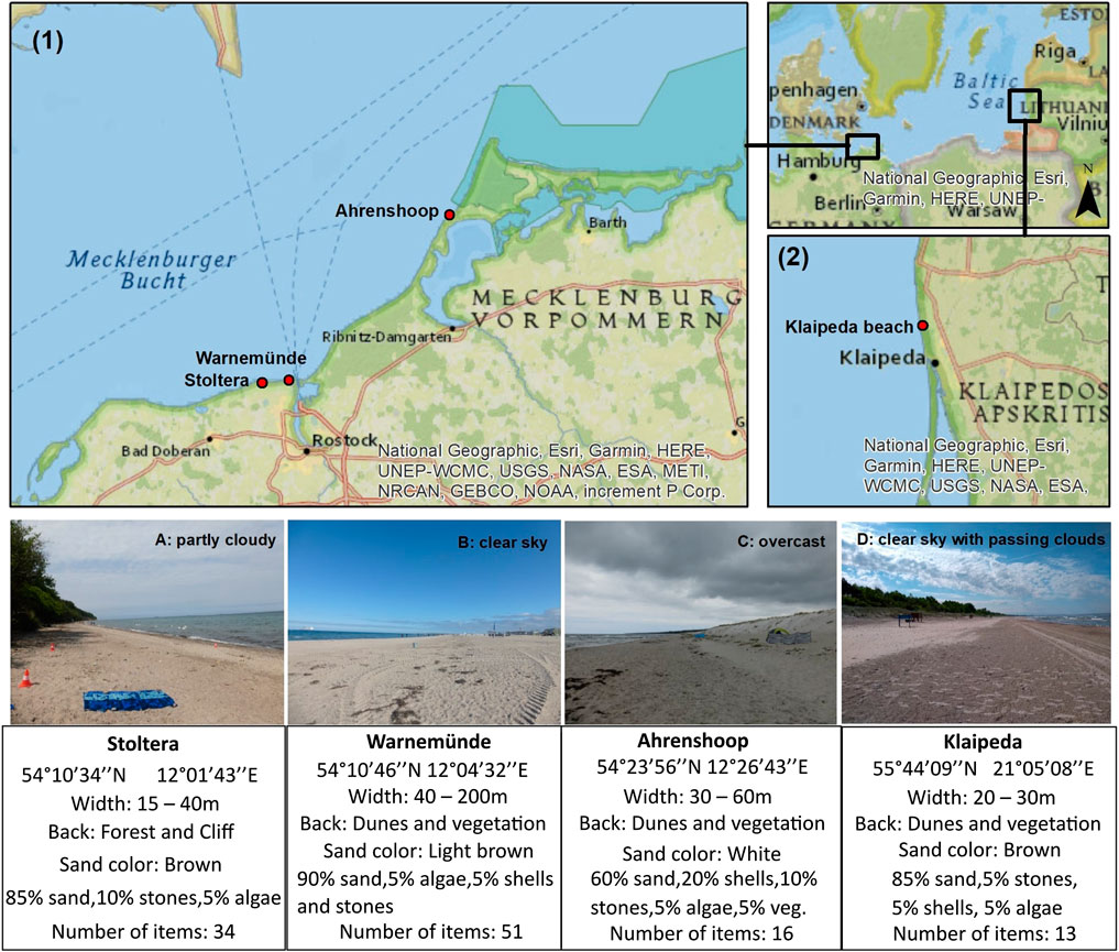
FIGURE 1. Study sites for drone mapping and in-situ data collection of beach litter in the Southern Baltic Sea, specifically Germany (1) (A): Stoltera, (B): Warnemünde, (C): Ahrenshoop) and Lithuania (2) (D): Klaipeda).

Aerial images were captured under different weather conditions (Figure 1). At all German beaches, official cleaning activities takes place regularly. In Stoltera and Warnemünde, cleaning occurred every day from 5–9 a.m. during high season and three times per week during low season. This is carried out with a mechanical vehicle (“Beach Tech 2000”) which removes litter and seaweed and is able to clean 22,000 m² per hour (pers. com. Rostocker Gehwegreinigung, July 2019; Tourismuszentrale, 2019). In Ahrenshoop, regular cleaning takes place by hand two times a week during high season (June–September) and no cleaning the rest of the year (pers. com. Kurverwaltung Ahrenshoop, October 2020). In Klaipeda, the beach belongs to the protected area “Coastal Region Park” and cleaning takes place only after extreme weather events (pers. com. A. Balciunas, 2019). In addition, removal of beach litter is also carried out by NGOs at all sites, serving as environmental awareness raising mechanisms (e.g., Battisti and Gippoliti, 2019).

Equipment and Software

Study areas were mapped with a low cost quadcopter DJI Phantom four Pro V2.0 with an integrated RGB CMOS camera of 20 Megapixels (focal length 8.8 mm) to develop and test an UAV-based approach for marine litter monitoring of meso- (1–25 mm) and macrolitter (>25 mm). The drone had a GPS/GLONASS system with a hover accuracy of ±0.5 m (vertical) and ±1.5 m (horizontal), a gimbal unit to provide near nadir observations and obstacle avoidance, automatic flight and Return To Home (RTH) features. A controller, which uses a smartphone device as display, allows monitoring of battery life and drone status. In this study, two smartphone devices (Android and iOS) were tested to run the flight mapping apps and fly the drone. PolarPro ND filters were used to adjust shutter speed under different light conditions, with ND 8 for cloudy, ND 16 for sunny and ND 32 for very sunny conditions.

For mapping, two apps were tested: DroneDeploy v.3.13.1 and Pix4D Capture v.4.5.0. The apps set the mapping area, flight altitude, speed, field of view (FOV), front and side overlap and create an orthomosaic with the images obtained. Agisoft Metashape was used for image stitching for one orthomosaic where neither of the mapping apps provided satisfactory results, using a standard process of photo alignment which uses images and point cloud data to create mosaics or 3D data (Agisoft, 2020). Moreover, the geospatial analysis software ENVI 5.3 and ArcGIS v.10.5 were used for image analyses. ENVI 5.3 served to explore the spectral signatures of different objects in the image, while ArcGIS v.10.5 was used to carry out supervised object-based classification.

Field Approach and Image Acquisition

The methodology for image acquisition and analysis followed five main steps (Figure 2). A total of four flights per beach (three for Klaipeda and Warnemünde) were carried out as one-time sampling in the same day at three different altitudes near the highest sun zenith angle (between 11 a.m and 1 p.m CET) in May, June, July and October 2019. All sampling was carried out under the permission of the Ministry for Energy, Infrastructure and Digitalization in MV, Germany and following the guidelines of the German Air Traffic Control (Deutsche Flugsicherung, DFS). In Lithuania, drone flights for small devices (<25 kg) do not require permission, thus sampling was not restricted but followed regulations (Civil Aviation Administration, CAA, 2020). Care was taken during all surveys to avoid impacts such as crashing on people or structures (e.g. trees), or cause disturbances to birds by the noise and start/landing of the drone. We carried out sampling away from conglomeration of people and chose a start/land site with sufficient distance from trees and structures. The drone was always kept on sight to maneuver in case of danger. The flight heights used were low and thus more noise was produced, but we kept flights short (3 min for recovery experiments and max. 20 min for one sampling of 100 m beach transect) to minimize disturbance. The sampling was carried out only under good stable weather conditions (noon, clear sky or homogeneous cloud cover, wind speed <20 km/h, no rain). Supplementary Table S1 shows the settings used for drone-based mapping following Martin et al. (2018) and own experiences. Ground Control Points (GCPs) were not used for georeferencing. The drone gives good positional relative accuracy- that is how points on a map are placed relative to each other- which we suggest is sufficient for image classification, as we are not overlaying different orthomosaics but rather making a comparison of the classification results between different flight altitudes and algorithms.

FIGURE 2. (1) Workflow for drone-based monitoring and object-based supervised classification based on five main steps, each with separate single steps to follow. (2) Set up for sampling of the recovery experiment (A) and 100 m beach transects (B). In the recovery experiments, selected items (based on most common items found in the Baltic region) were placed in a cleaned area of 5 × 10 m. The 100 m monitoring was based on OSPAR guidelines. After drone mapping of the zone, litter was collected on the area from the intertidal to the back of the beach with two people and then counted and classified according to the OSPAR list of items.

Previous studies using consumer drones with a camera resolution similar to ours, tested flight altitudes between 5 and 35 m (Deidun et al., 2018; Martin et al., 2018; Fallati et al., 2019) and up to 60 m (Atwood et al., 2018; Goncalves et al., 2020). The flight altitudes chosen for this study were set based on the Pix4D Ground Sampling Distance (GSD) calculator to obtain a GSD <5 mm as optimal spatial resolution to detect litter in the meso (5–25 mm) and macro (>25 mm) scale; namely 10, 15, and 18 m, which would give spatial resolutions of 2.7, 4.1, and 4.9 mm, respectively. This is also in accordance with the EU law regulations for drone flights, limited to a range of 10 m to 120 m, based on the aircraft settings and EU law (European Parliament and Council, 2018).

To assess the detection accuracy of litter items at these different flight heights, recovery experiments were carried out on a previously cleaned area of 5 × 10 m (Figure 2) where litter items of different colors, shapes and sizes (1–30 cm) were displayed (Supplementary Figure S1). These included the most common item categories for the Baltic (Schernewski et al., 2017). The sites mapped had different number of items (14–57 items) and background substrates and were sampled under different weather conditions (Figure 1). In addition, beach transects of 100 m (with unknown number and type of litter) were mapped from the intertidal zone to the back of the beach (Figure 2) at a flight height of 10 m. After mapping, two people collected the items seen by naked eye and classified them according to the OSPAR list of items (OSPAR, 2010). All captured images were converted into orthomosaics and these were integrated in a Geographic Information System (GIS) for image analyses.

Image Processing and Pre-analyses

A total of 14 orthomosaics were created in GeoTIFF format which presented spatial resolutions of 2.7–8 mm/px, based on flight height and mapping app used. In general, all apps use photogrammetry approaches based on image orthorectification with point clouds and elevation data to produce orthomosaics, however, different image processing may have caused the differing spatial resolutions between the apps (e.g., use of image stitching enhances image spatial resolution). For each site, three orthomosaics (one for each flight height) of recovery experiments (Klaipeda and Warnemünde, only two) and one orthomosaic of a 100 m beach transect taken at 10 m altitude. Image analysis was carried out on ArcGIS, using Digital Numbers (DN) with a radiometric resolution of 8 bit. The projection used was WGS1984 UTM Zone 33N/34N for Germany and Lithuania, respectively.

First, the orthomosaics obtained from the recovery experiments at 10 m height were visually screened to assess and compare the accuracy of litter detection from drone imagery vs. ground truth data. Here, the analyst knew the number and type of items but not their position in the image. The items were counted from left to right, starting at the top of the image towards the bottom, zooming at the objects to mark them. Preliminary analyses were conducted to find the best classification method between pixel-based vs. object-based classification. Similarly, the influence of different number of classes (2, 4, and 6 classes) was tested in ArcGIS and ENVI. The latter was used to inspect the spectral differences of each background material by taking 10–20 samples of objects in each orthomosaic.

Object-Based Supervised Classification

Image classification followed a standard procedure of object-based supervised classification incorporated in ArcGIS including four steps, i.e. segmentation, the selection of training samples, classification and accuracy assessment.

Segmentation groups pixels into “objects” based on homogeneity criteria set by spectral and spatial values and minimum segment size. This aims at reducing noise from the background and highlighting objects of interest for object-based classification. Based on the gained knowledge from the investigated sites, a decision tree for choosing segmentation parameters was created (Figure 3). Spectral and spatial values were chosen individually per site. The minimum segment size used here was between 2 and 10 pixels (1–5 cm²) with the aim to allow recognizing small litter items like cigarette butts (1–2.5 cm). It is important to consider that only four beaches were studied, thus the employment of this decision tree should be further tested for its application in more sites. For an example of the segmentation result, see Supplementary Figure S2.

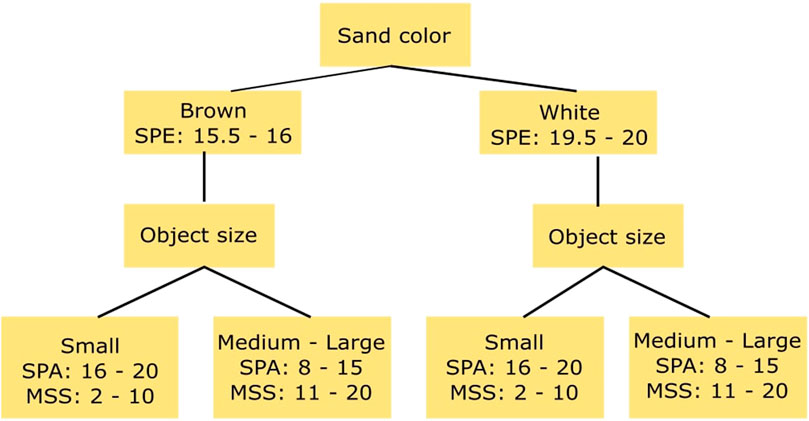
FIGURE 3. Decision tree for segmentation parameters based on beach characteristics of the four study sites. SPE: Spectral Value, SPA: Spatial Value, MSS: Mean Segment Shift Value.

The classification approach used is supervised and therefore requires training data. Training samples were taken as segments to obtain 4–6 distinct classes. The criteria used here were: 1) select >20 samples (if possible), proportional to the class size but not exceeding the number of objects per class in the image, 2) select samples with enough distance from one another to increase variability of the training set, 3) select samples at the center of the item to avoid mixed pixels and 4) include different color tones for each class, i.e. if vegetation was present in different tones of green, training samples included these to provide an accurate classification of the class. Additionally, histograms and scatterplots on ArcGIS were checked to ensure that each class was spectrally distinct from one another. The training samples taken at each recovery experiment were used for classification of the recovery sites and 100 m beach transects.

Three supervised classification algorithms were tested: Maximum Likelihood (ML), Random Forest (RF) and Support Vector Machine (SVM). These algorithms follow different set of rules in respect to the training samples to be used. For the RGB camera used, ML classification in ArcGIS requires a minimum number of 20 training samples per class and assumes normal distribution of the samples, while RF classification and SVM can work with fewer samples, do not assume normal distribution and are less susceptible to noise in the image. The functioning of each algorithm is also different. ML is based on the concept of normal distribution and Bayes theorem of decision making, based on the probability that every pixel in an image belongs to a particular class. The strength of ML is that it considers the variability within each class using the covariance matrix to classify the candidate pixel (Lillesand et al., 2004). RF uses multiple decision trees trained to use small variation of the data, where the majority vote from the trained trees decides the class assignment for each pixel (Berhane et al., 2018). SVM is a non-parametric statistical learning approach and therefore there is no assumption made on the underlying data distribution. SVM maps input data as vectors into a higher dimensional space to separate data into different classes using hyperplanes (Mountrakis et al., 2011). The output of the approaches is a classified image (.tif) of a number of classes as defined in the training samples.

Accuracy assessment of the image classifications was carried out with a set of 500 validation points created in an “equalized stratified random” manner, i.e. distributed within each class, each one having the same number of points. A confusion matrix, based on the comparison between the classification and reference data, revealed the accuracy of each algorithm by calculation of commission and omission errors for each class, total accuracy and kappa value of agreement. The total accuracy (TA) is the percentage of correctly classified validation pixels and measures the accuracy of the classified image. The producer’s accuracy (PA), also known as recall, indicates the true positive rate or the proportion of true positives in relation to true positives and false negatives in the model classification. It is also a measure of omission error. The user’s accuracy (UA), also known as precision, indicates the positive predictive power or the proportion of true positives in relation to true positives and false positives in comparison to the reference data. It is also a measure of commission error (Story and Congalton, 1986; Campbell and Wynne, 2011). Cohen’s Kappa gives an overall assessment of accuracy of the classification in respect to randomness, with a value of 0 indicating no better than random, >0 better than random and <0 worse than random (Cohen, 1960).

Because only one replicate classification was carried out per height and algorithm, statistical tests for significant differences were not conducted. Instead, we provide an overview of the accuracy measures obtained from each image classification and a comparison of the mean and standard deviation between the classifications at different flight heights for each sampling site.

Cost-Efficiency Analysis

Official marine litter monitoring methods need to be time and cost efficient. The MSFD requires the comparison of methods for marine litter monitoring to meet the practical demand of cost-efficiency (JRC, 2013) considering implementation and annual running costs to fulfill the MSFD Descriptor 10 and to be implemented by national authorities within their national marine litter monitoring programs. The following approach provides a subjective comparison of a set of two monitoring methods: an UAV monitoring method with a commercial RGB drone and a hypothetical non-established spatial-OSPAR monitoring method to evaluate aspects of costs and efficiency. The evaluation of efficiency was based on four criteria: accuracy, reproducibility, flexibility and quality. Accuracy refers to the share of items identified at the beach transects vs. ground truth data. Reproducibility reflects the likelihood that, when a method is applied by different persons, drones and software, the same results will be obtained. Flexibility is defined as how flexible the method is with respect to weather conditions, external disturbances, permissions and battery life. Quality refers to how well are items defined and whether sufficient data is provided, i.e. type and number of items, type of material and spatial distribution.

In contrast to the current OSPAR method, spatial-OSPAR considers the spatial distribution of litter items per area, thus comparable to the output of the drone approach, and taking into account 100 m beach transects (or 1 km beach transects for items >50 cm) with smaller transects of 10 m and 3–6 quadrats of 9 m², displayed from the tide line, middle and to the back of the beach (an adapted version after Bravo et al., 2009).

Costs of the UAV and the spatial-OSPAR methods were calculated considering implementation costs (equipment, software and testing period) and annual running costs for office and field/lab work to be carried out at four beaches, four times a year, by a minimum of two persons. Our time and costs estimations follow own experiences. These estimations may, therefore, vary based on type of drone used, analysis method and level of training required, as well as currency and salary estimations for the country. The initial costs include equipment costs as well as the costs for a testing period for both methods (6 months for the UAV-method and 3 months for the spatial-OSPAR method). Annual running costs include field/lab (travel, survey and analysis) working time and office (planning, organization and reporting) working time. The total monitoring costs were calculated as the sum of initial costs and annual running costs for field/lab and office work, and were classified as: 5 (very low) < 15,000 €; 4 (low) < 30,000 €; 3 (moderate) < 45,000 €; 2 (high) < 90,000 € and 1 (very high) > 90,000 €.

Each method and criteria was scored separately, evaluated by three experts as: 1 (very low), 2 (low), 3 (moderate), 4 (high) and 5 (very high). The efficiency score is the average of the scores for each criterion. To obtain the final cost-efficiency score, the cost and the efficiency scores were multiplied and classified as: <5 (very low), <10 (low), <15 (moderate), <20 (high) and >20 (very high).

Results

Preliminary Analyses

Accuracy Assessment by Visual Screening

Visual screening carried out on images captured at 10 m flight height revealed a mean recovery rate of 99.4 ± 16.2% for the four beaches (Ahrenshoop 87.5%, Stoltera 97%, Warnemünde 90%, in Klaipeda 16 instead of 13 items were found again, 123%). These results gave the first “green light” towards testing a semi-automatic method for classification with ArcGIS. The objects easier to find by visual screening were larger items (>2.5 cm), items placed close to each other, items of bright colors and shapes normally not found naturally at the beach (e.g. bottle caps in yellow, blue, pink, orange, red, bright green). The objects most difficult to find were mainly in colors white, black, brown and transparent and shapes like string/cord, lines and squares, especially of small sizes and diameters (<2.5 cm).

Pixel Based vs. Object Based Classification

The high spatial resolution of drone images, which is needed for the detection of small litter, also led to noise from shadows, differences in sand color and tread marks, which disturb the classification, and thus needed to be handled accordingly. Pixel-based unsupervized classification (A) resulted in a complex image due to high variations on sand, background substrate (i.e. sand color and amount of stones, shells and vegetation), colors and shades. Using object-based unsupervized classification (B) objects were clearly separated from sand and the “noise” from shadows and differences in sand color were reduced or eliminated (Supplementary Figure S3). The results of this test classification also showed that images at 10 m height gave a closer and sharper look into smaller objects than images obtained at 15 and 18 m height (Supplementary Figure S4), which reduced the noise of the background but smaller objects were more difficult to identify and classify.

Influence of Different Number of Classes

Unsupervized classification into two classes highlighted all objects from sand (Supplementary Figure S5A), whereas classification into four classes (Supplementary Figure S5B) showed clustering of the objects, however with high variability in the classification, i.e. one object was classified as three different ones. The classification into six classes showed even higher variability in the classification: objects of white and black color were clustered separately and colorful litter items were highlighted from the sand but classified in non-coherent clusters with single items belonging to more than one class (Supplementary Figure S5C).

The analysis of spectral profiles of objects on ENVI 5.3 revealed that each object had a different spectral profile and could therefore be classified separately into a total of maximum six classes: litter, algae, vegetation, shells, stones and sand. For Warnemünde, the class “shadows” was added (Supplementary Figure S6). Between all classes present, algae, vegetation and sand presented characteristic and consistent spectral profiles that could allow the differentiation from other classes. However, for the case of litter the high variation in color presented no consistent curve in which classification could be based upon. Lastly, shells, stones and shadows that were present in either white or dark colors had similar spectral profiles with flat DN values at either extreme (0–255).

Like this, four to six classes were chosen for the selection of training samples to carry out object-based supervised classification with three algorithms. For classification with four classes, algae and vegetation as well as stones and shells were considered together as two classes. For classification with six classes, algae and vegetation as well as stones and shells were considered as separate classes. This latter classification was carried out only for the sites where the presence of stones and shells as well as of algae and vegetation was clear, in this case Stoltera and Ahrenshoop. Although these classes are not the object of interest, it was important to understand how white and black objects would be classified.

The criterion to “select >20 training samples” was not possible to fulfill in all beaches and taking a larger amount of training samples in the small recovery area contradicted the goal of the semi-automatic classification. For the object of interest (i.e. litter), most beaches had at least 20 training samples. For Klaipeda, which had the lowest density of litter in the recovery area, 10 training samples were chosen. Since stones and shells were not easy to distinguish from white or black objects (e.g., litter or algae pieces) from the spectral profiles, only a few samples were taken based on their shape and distance from algae or water, to avoid misclassifications.

Object-Based Classification

The accuracies of image classification for recovery experiment (5 × 10 m) are shown in Table 1. The classification with four classes showed total accuracies (TA) that ranged between 36% and 90% for ML, 54% and 73% for RF and 44% and 76% for SVM, depending on flight height and site. Producer’s accuracy (PA) for litter showed similar ranges: 45–100% for ML, 67–95% for RF and 61–100% for SVM. Whereas user’s accuracies (UA) for litter were lower. Kappa values were in most cases >0.60 indicating that classification was better than random. Classification with six classes showed in general lower values for TA, PA and UA for all algorithms and sites. Here kappa values were in most cases <0.60 indicating that classification was closer to random.

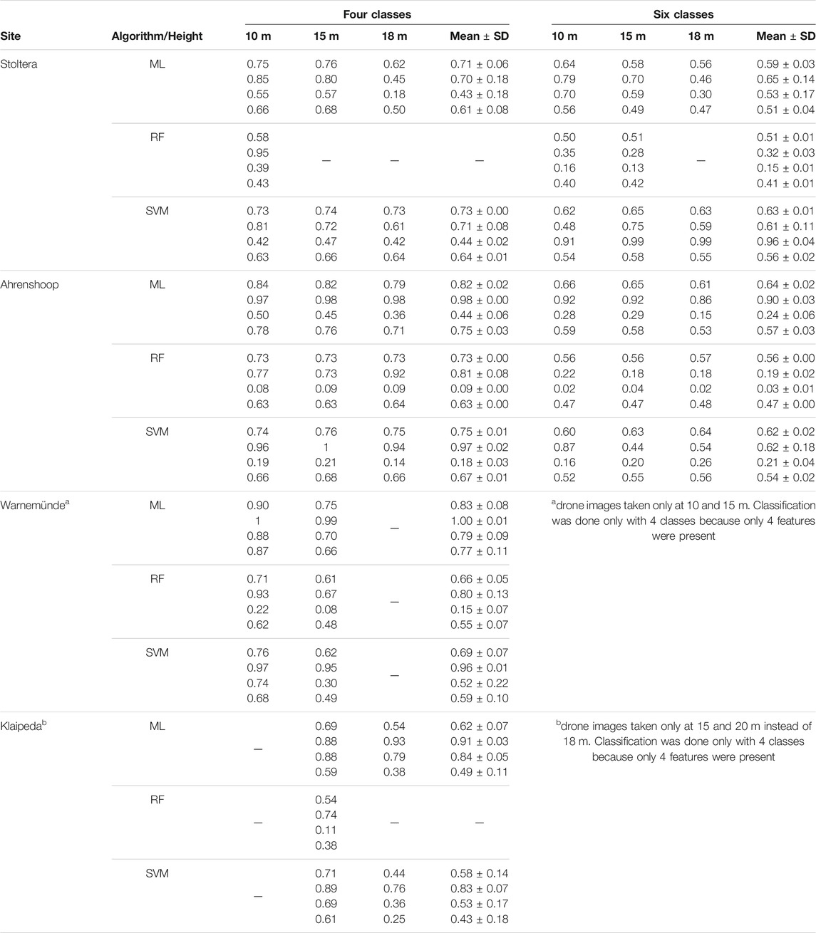
TABLE 1. Accuracy of image classification on recovery sites with 4 and 6 classes (litter, vegetation, algae, stones, shells and sand) for each site, algorithm and flight height. The values are presented as percentage from top to bottom: Total Accuracy (TA), Producer’s accuracy (PA) of litter class, User’s accuracy (UA) of litter class and kappa value of agreement (k).

In most cases, measures of accuracy (TA, PA, and UA) decreased at images taken at higher flight altitudes. Classification of images taken at 10 m showed highest TAs, highest PA for litter classification and highest kappa values in most sites for the three algorithms. In some cases, higher TAs were also seen at images taken at 15 m or 18 m; however, this was mainly due to higher accuracies in classes other than litter. User’s Accuracy (UA) for litter was lower for all classification algorithms, with values of 18–88% for ML, 8–39% for RF and 14–75% for SVM with four classes and 15–70% for ML, 2–16% for RF and 16–99% for SVM with six classes, depending on flight height and site (Table 1).

Due to a lack of replicates, an assessment of significant differences for measures of accuracy between algorithms was not possible to carry out and thus is not possible to statistically assess if an algorithm performs better than another. Nevertheless, Table 1 shows that no clear differences were found between algorithms for samples taken at different sites. Similarly, no clear differences were observed between measures of accuracy for images taken at different heights, which in general showed low standard deviations from the mean.

The resulting classified images showed that ML and SVM gave a better representation of litter and background features in contrast to RF (Figure 4). In the case of Warnemünde, similar classifications were seen between the three algorithms but SVM showed misclassifications between vegetation/algae and shadows (Figure 4). For 6-class classification, these results were similar, but as more classes were used, more detail was defined and misclassifications were seen between shells and white litter objects (Figure 5). In general, both ML and SVM were able to classify meso- and macrolitter size with varying accuracies relative to sand color, background substrate, weather conditions and litter objects.

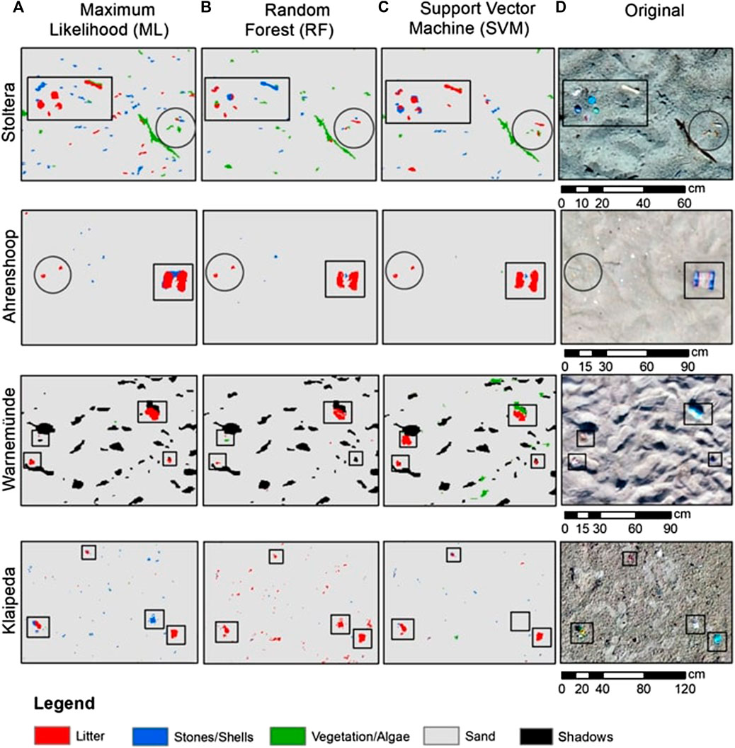
FIGURE 4. Comparison of supervised classification with four classes with the algorithms ML, RF, and SVM on erial images at 10 m for the site Stoltera, Ahrenshoop, Warnemünde and Klaipeda. Each close-up image shows litter objects on the recovery site (D) and their classification result (A–C), such as litter objects of different sizes (square) and cigarette butts (1–2.5 cm) (circle).

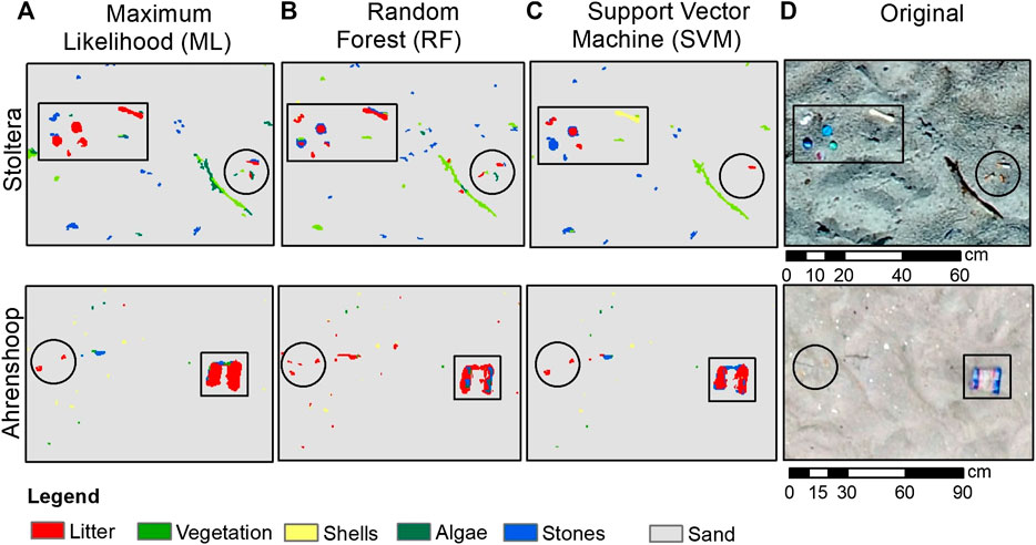
FIGURE 5. Comparison of supervised classification with six classes with the algorithms ML, RF, and SVM on erial images at 10 m for the site Stoltera and Ahrenshoop. Each close-up image shows the distribution of litter objects on the recovery site (D) and their classification result (A–C), such as litter objects of different sizes (square) and cigarette butts (1–2.5 cm) (circle).

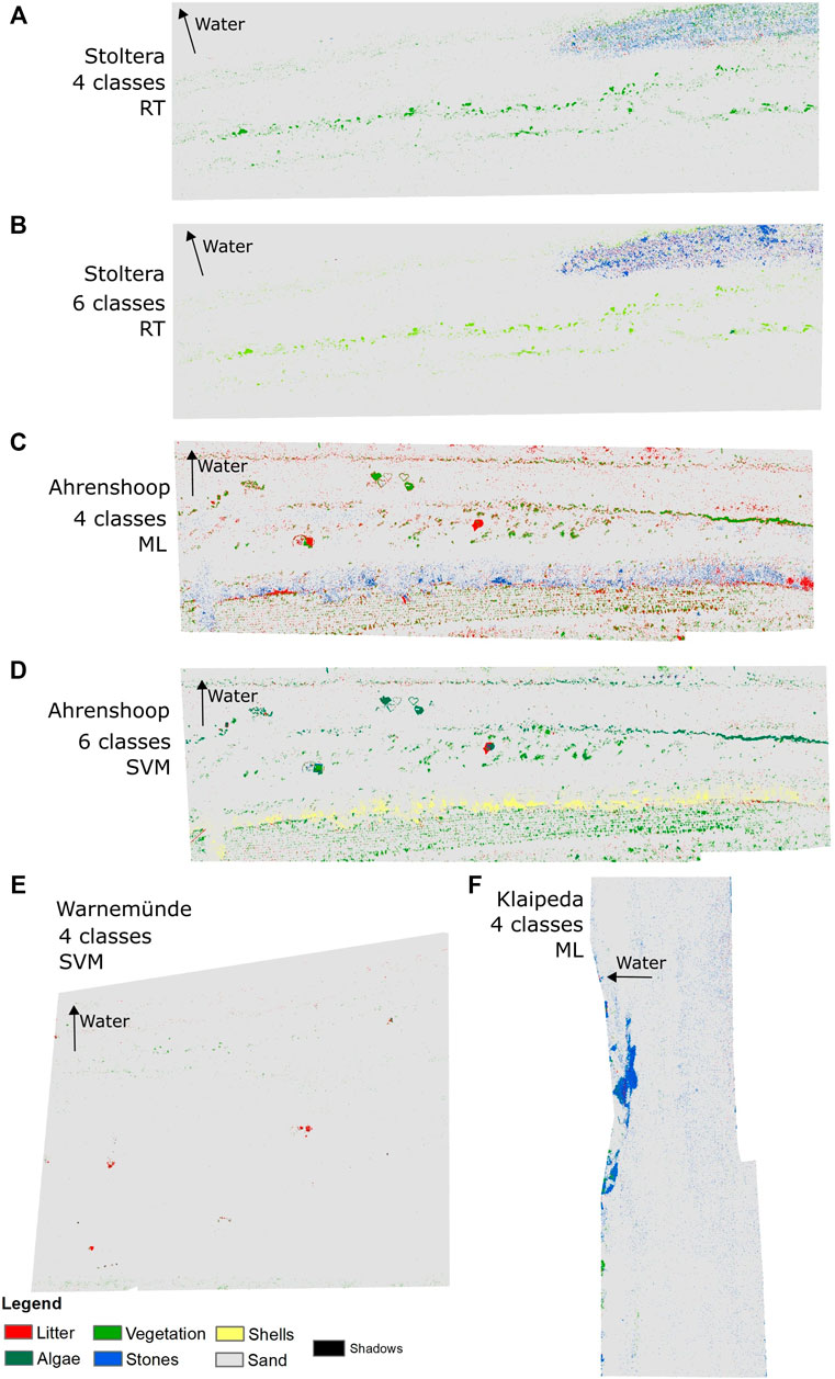
FIGURE 6. Object-based supervised classification of 100 m beach transects taken at 10 m flight height. Only the results with best total accuracy (TA), producer’s accuracy for litter (PA) and kappa value of agreement for with 4 and 6 classes are shown for each site: Stoltera (A,B), Ahrenshoop (C,D), Warnemünde (E) and Klaipeda (F).

The classification of 100 m beach transects (at 10 m flight height for German sites and 15 m for Klaipeda) showed lower accuracy values than achieved on the recovery experiments, independent from site and image resolution. Classification with four classes showed kappa values between 0.23 and 0.53, which indicated that classification was rather random among different algorithms and no single algorithm could show a good performance in all cases (Table 2). Similar patterns were seen for the classification with six classes. The high range of difference for PA and UA for litter is due to how AAPs are placed on the image, sometimes hitting only one or no litter item, which skewed the results to either extreme (0 or 100%).

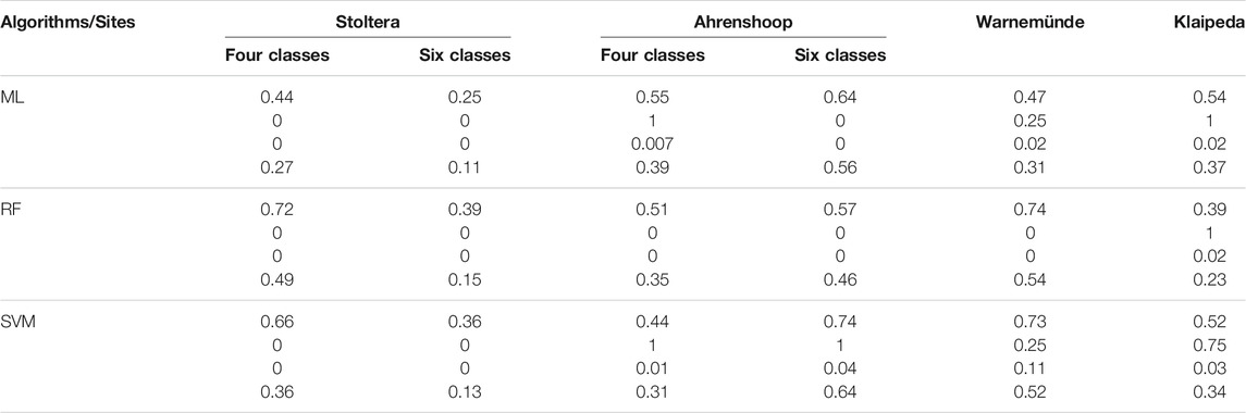
TABLE 2. Accuracy of image classification on 100 m beach transects at 10 m flight height with 4 and 6 classes (litter, vegetation, algae, stones, shells and sand) for each site, algorithm and flight height. The values are presented as percentage from top to bottom: Total Accuracy (TA), Producer´s accuracy (PA) of litter class, User´s accuracy (UA) of litter class and kappa value of agreement (k).

The classified 100 m beach transects showed similar classification patterns as in the recovery experiments but could not be representative of the litter found on the sites during collection (Stoltera: 174 items, Warnemünde: 167 items, Ahrenshoop: 77 items and Klaipeda: 214 items) (Supplementary Figure S7). Figure 5 shows the classification results with highest TA, PA for litter and kappa values for each site (seen at Table 2). Both images and confusion matrices showed that misclassifications occurred in all algorithms (Supplementary Table S2). ML showed misclassification between litter and vegetation in Warnemünde (Supplementary Figure S12) and between vegetation, stones and litter in the classification with four classes in Ahrenshoop (Supplementary Figure S10). RF showed an overestimation of litter abundance in Klaipeda (Supplementary Figure S13) and in the classification with six classes in Ahrenshoop (Supplementary Figure S11). SVM misclassified vegetation and litter in Stoltera (Supplementary Figures S8, S9) and stones and litter in Klaipeda (Supplementary Figure S13). Objects that were correctly classified were anthropogenic items (beach tents of ca. 2 m in Warnemünde–Supplementary Figure S12—and Ahrenshoop–Supplementary Figures S10, S11 classified as litter), algae and beach wrack in Stoltera (Supplementary Figure S8) and Ahrenshoop (Supplementary Figure S10), vegetation (Supplementary Figure S10) and shells (Supplementary Figure S11) in Ahrenshoop, and stones in Klaipeda (Supplementary Figure S13).

Time and Cost-Efficiency

As seen on Table 3, the UAV spatial method for 100 m and 1 km beach monitoring involves higher initial costs and about two times more costs and time effort for field work and analysis than the spatial-OSPAR method. The higher investment costs for the UAV method are related to software costs, since license software is often required within official federal agencies. If these software costs were not considered, the investment costs would decrease to only 3,000 € for the drone and other materials. Costs for testing period of implementation were higher for the drone method, estimated as 30,000 € for the 100 m and 1 km monitoring vs. 15,000 € for the spatial-OSPAR method. Office costs are the same for both methods. Annual running field costs (survey on site) were lower for the UAV method at 100 m beach transects (1,800 € vs. 2,400 € for the spatial-OSPAR), but higher once spatial extension increased to 1 km (2,400 € vs. 1,800 € for the spatial-OSPAR method). Annual running costs for analysis of the data (lab work) was considerably higher for the UAV method than for the spatial-OSPAR method (4,800 € vs. 2,400 € for 100 m and 9,600 € vs. 1,200 € for 1 km) (Table 3).

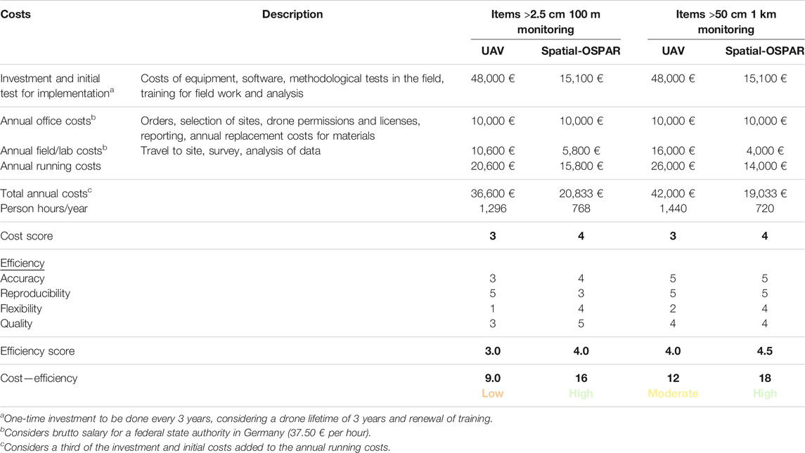
TABLE 3. Cost-efficiency analysis for UAV and spatial-OSPAR for beach litter monitoring methods. The values are based on our experience taking into account the MSFD guidelines (JRC, 2013) and federal state authority staff salaries (37.5 € per hour) for a monitoring of four beaches, four times a year. In bold are shown the scores for cost and efficiency, giving the cost-efficiency score.

The overall cost-efficiency score for beach litter monitoring was 9–12 (low to moderate) for the UAV method vs. 16–18 (high) for the spatial-OSPAR method.

Discussion

Lessons Learned From Object-Based Classification

Results from the recovery experiment showed that litter sizes >2.5 cm (i.e. macrolitter size) were the minimum size detectable. PAs for litter for the recovery experiments at different sites were between 77% and 100% with kappa values between 0.43 and 0.87 for images taken at 10 m height. These accuracy values were comparable to those obtained through visual screening of the same images (>87%, mean 99.4% ± 16.2). Even if smaller litter items were detected and classified (e.g., Figures 4, 5, cigarette butts <2.5 cm), in reality many were misclassified. Another study also showed limitations in the detection of smaller items size, where items <4 cm were also most misclassified (Martin et al., 2018). TA was lower for classification into six vs. four classes (Table 1), but the PA for litter was in some cases similar, reaching values between 70 and 80%. In the 6-class classification, white and dark litter items were better classified than with the 2-class or 4-class classification (Supplementary Figure S5), but at the same time introducing more classes increased the complexity of the image.

The results from visual screening and spectral curves gave an initial indication of misclassification. Objects with a flat spectral curve (e.g. white shells and black stones) in colors white, black, transparent and brown, and litter which did not present any consistent curve (Supplementary Figure S6) were most misclassified on RGB images, whereas the objects of bigger size (>2.5 cm) and bright colors were correctly classified as litter (e.g. Figure 4). This is because object color, weather, light conditions and background substrate influence DN values and thus classification. In addition, the selection of training samples based on DN values depends on the judgment of the observer, increasing chances of error and misclassifications. Furthermore, it was not possible to establish whether one algorithm can cope better with background complexity than others, since factors like weather conditions differed in each site. We suggest that the higher complexity of sand and background substrate challenges segmentation of the image, which in turn, influences classification results. This was also observed by Martin et al. (2018) where shadows, vegetation and non-uniform background as well as the variability of each item within the same category (different sizes and colors) presented limitations in classification. In our study, as complexity of the background increased, the use of more classes became beneficial (e.g. in Ahrenshoop, Supplementary Figures S10, S11). However, in order to derive accurate statistics, the use of replica on each site and condition as well as further explore the influence of litter quantities and background substrate should be explored.

No clear differences of performance accuracy could be assessed between the algorithms; however, in contrast to previous studies, RF was the algorithm that presented most problems in performance in our images (Table 1). Martin et al., (2018) used RF classification obtaining an accuracy of 61.8% for detection of litter, 39.5% total accuracy and F-score of 0.13. Their classification presented an overestimation of 5-times due to false positive items, as similarly seen in the classified images with RF in our study. Another study by Goncalves et al. (2020) at beaches in Portugal also used RF, obtaining 75% sensitivity (≈Producer’s accuracy) and 73% positive predictive value (≈User’s accuracy) with a F-score of 0.75. These studies used approaches related to changes in the color space of spectra (Martin et al., 2018; Goncalves et al., 2020) which were not used in this study.

Observations of the classified images from recovery experiments suggest that ML better highlighted small features (stones or shells) (Figure 4, 5) but did not necessarily classify litter better (Table 1), yet bottle caps and larger macrolitter were detected. In contrast, SVM gave less importance to small features leading to less noise from stones, shells or sand heterogeneity within the images. Still, small objects (also litter) were well classified in most cases, up to large mesolitter sizes like cigarette butts (Figures 4, 5). Some studies suggest that a higher litter abundance leads to higher detection of litter by RF and other algorithms (Martin et al., 2018; Atwood et al., 2018), which was not observed in our study.

The image classification used in this study did not provide a distinction of litter composition and only focused on detection of litter items to provide an estimation of abundance and distribution. Based on the litter collected on site, the highest amounts of litter were in the categories plastics and paper (mainly due to cigarette butts), mainly macrolitter size of white or brown color and colorful mesolitter items (Supplementary Figure S7). Our results showed, however, that GIS classification based on RGB data was not satisfactory to provide estimations of abundance, since litter items were not possible to identify from the classified images at large spatial scales (100 m beach transect). TAs at the 100 m beach transects were much lower than at recovery experiments and PAs for litter were in most cases 0% (Table 2). This may be due to uncertainties in the method, because accuracy assessment depended on whether one or more points hit a litter object or not, bringing accuracy to extreme values of 0 or 100%. Due to the low segment size used for segmentation, large items were constructed with several segments, thus litter “objects” could not be counted as such in the classified images since the number of segments per item would overestimate the real count. Future studies should consider taking the GPS coordinates of litter items as a method to get reference data for larger transects.

Our analysis method did not prove to be sufficiently accurate or time-efficient. It is important to consider other methods for analysis, while following requirements for official beach litter monitoring. As technology develops and advanced equipment becomes more accessible, many of the limitations encountered in our study (mainly related to image resolution and processing time) will be overcome. Other methods including deep learning have demonstrated to be an alternative for the classification of objects on RGB images since it does not rely only on DN values (Fallati et al., 2019). In their study, object recognition reached a sensitivity (≈Producer’s accuracy) of 67%, positive predictive value (≈User’s accuracy) of 94% and F-score of 0.49, arguing the tool can be well used for the monitoring of litter and detection of hotspots in the study sites.

Strengths and Limitations of Consumer Drones for Beach Litter Monitoring

Taking into account our experiment results and assessment on cost and time efficiency, drones are still a method that needs to be explored and adjusted for efficient monitoring. The images from drones provide high spatial resolution which is required for the detection of small litter items. Our results showed that litter sizes >2.5 cm (i.e. macrolitter size) were the minimum size detectable. Even if smaller litter items were detected and classified (e.g., Figure 4, cigarette butts <2.5 cm), in reality many were misclassified. Thus, the accuracy of consumer RGB drones can be regarded as high (Table 3) for large particles but decreases with smaller item size and additionally depends on parameters such as item color, shape and weather conditions. These limitations could be overcome with more advanced drone sensors (e.g. multispectral) or the use of other analysis methods (e.g. deep learning) which increase accuracy; however, this would involve higher costs and expertize. In terms of type of data obtained and quality, our results suggest that the drone method (with RGB camera) can only provide data on the number of items and spatial distribution (moderate to high quality), in contrast to the spatial-OSPAR method where litter objects are collected by hand and can be better visualized to define also type of item and material, and give indications of pollution sources (Table 3).

A clear strength of drones is reproducibility (Table 3). Our results showed that the mapping of sites can be easily carried out after simple training of staff with the help of free mapping apps. These apps automatically map a site of interest at a set height, speed and area, enabling long term monitoring of the same site under consistent conditions. Although our analysis method did not prove to be sufficiently accurate and time-efficient, analysis of data in general would follow a strict protocol, carried out semi-automatically, decreasing chances of human error once the method is set up and sufficiently evaluated. For the 100 m OSPAR beach monitoring it is known that a difference of at least ± 10% is common, depending on who is carrying out the field work (Schernewski et al., 2017). In this respect, the drone method shows very high reproducibility in contrast to moderate reproducibility for the spatial-OSPAR method, and comparable values for 1 km beach transects (Table 3). Nevertheless, our own experiences showed that drone and GIS based monitoring is time-intensive (creation of orthomosaics 2–8 h, classification of the images, 3–8 h) and analysis of the images requires higher skills than for data obtained with an adapted spatial-OSPAR method.

Flexibility was the main limitation for monitoring with commercial drones in contrast to current monitoring methods (Table 3). The drone method depends on wind, weather and light conditions and can hardly be applied according to a fixed timetable. However, the dependence on weather conditions is a factor that all remote sensing studies need to consider (Murphy, 2015). At our study sites, ideal weather conditions initially involved wind speeds <20 km/h and enough sun light; however, overcast conditions and wind speeds of 27 km/h at Ahrenshoop also demonstrated good results (Table 1: Figures 4, 5). Cloudy conditions showed best image outputs to avoid direct sunlight and shadows which led to sun glint and darker areas that disturbed image classification (Supplementary Figures S8, S9). ND Filters helped to minimize the reflection from sand under strong sunlight but shadows and sun glint could not be fully corrected. Issues with GPS signal, battery life (max. 20 min) and compatibility between smartphone device and mapping apps were also limitations encountered during our sampling. In addition, drone licenses are nowadays needed for all types of aerial drones and legal permissions are required at most places in Germany and limited to zones outside nature protected areas and of high urban density or conglomerations of people (§ 21a LuftVO, BMVI, 2017). From December 31, 2020, new EU regulations will apply and replace national regulations for each country (European Union Avitation Safety Agency, 2020).

Another important factor to discuss is the common natural trade-off of remote sensing approaches where decreasing flight altitude increases image resolution, but also decreases the area of coverage, increasing post-processing times and costs (Murphy, 2015). The large number of images obtained (44–234 images for recovery experiments and 459–1,247 images for 100 m beach transects) at 10 m led to high processing time for orthomosaic creation (12–24 h). Drone images in our study had a high spatial resolution (2.7–8 mm, 20 MP camera) and litter objects were possible to see on images taken at all flight heights, but higher flight altitudes (e.g., 18 m) were not enough to classify objects (i.e. stones, shells, vegetation) accurately. Low flight height has also been related to blurry images and vigneting effect especially on sites with homogenous ground, like sand, which hinders orthomosaic construction (DroneDeploy, 2020). Studies that carried out mapping at much higher altitudes, focused on litter patches or much larger litter at the coastline or rivers (Atwood et al., 2018; Deidun et al., 2018) or combined geomorphological and hydrodynamic variables into one model that allowed more specific detection (Goncalves et al., 2020).

Contrarily to our results, a recent study using a similar set up suggests drone survey to be a cost-efficient method for litter quantification, however their study inspects a beach area of 20 × 20 m by visual screening done by people (Lo et al., 2020). The higher costs, and thereby lower cost-efficiency suggested in our study are likely related to the method used for analysis and the larger areas of beach inspected, as required by OSPAR (2010).

The main constraint for remote sensing of plastic litter is the various shapes, dimensions, colors and materials in which litter is present, making its recognition complex. Litter that is partially or completely buried or hidden between the back vegetation are not easily detected (Kataoka et al., 2018), especially with colors white, black, brown and transparent, as seen in our study. NIR spectroscopy with a MicroPhazir hand-held device is used to complement OSPAR studies and obtain more detailed information on material composition of mesolitter (Haseler et al., 2018; 2019); however, to our knowledge there is no published study using multi- or hyperspectral data on drones for the purpose of marine litter monitoring. Methods by Acuña-Ruz et al., (2018) used supervised classification for the detection of Styrofoam and other macrolitter items (>0.5 m²) on hyperspectral data using Visible and Near Infrared (VNIR), Short Wave InfraRed (SWIR) and Thermal InfraRed (TIR) wavelengths of satellite imagery for the creation of a spectral library of macrolitter items and natural features at the beach (e.g., sand, algae, stones and shells) for classification. The spectral signature of marine plastics has shown to have three absorption features at 1,215 –1732 nm (Garaba et al., 2018) as well as 2,313 nm specifically for PE (Levin et al., 2006) and between the blue and green bands and NIR spectrum for the detection of Styrofoam and other macrolitter items at the beach (Acuña-Ruz et al., 2018). Although the use of multi- and hyperspectral data can provide more detailed data, it also implies higher costs due to equipment and expertize needed.

Application of Aerial Drones as Official Beach Monitoring Methods

The MSFD encourages developing a comprehensive knowledge on the sources and sinks of marine litter to adopt policies that adapt to its current status. In the OSPAR guideline, currently in use at the Baltic, trends on abundance and types of litter are assessed every 3 months (OSPAR, 2010). Fulfilling the requirements from the MSFD and carrying out monitoring for all marine compartments to get a complete overview of the marine litter problem can be challenging in time and cost efforts. The data acquired needs to be reliable and accurate for the design of mitigation strategies. With drone-based monitoring, efforts during sampling can be reduced and the fatigue aspect and visual differences can be eliminated if automatic detection is carried out. However, as it is common when using remote sensing approaches, implementation costs for the drone-based method are higher (Murphy, 2015) in contrast to OSPAR, as also seen in our results. In addition, the skills needed for analysis require prior professional training and longer processing times, leading to higher annual running costs. Furthermore, the drone-based method requires the removal of litter, when carried out within a monitoring program. Thus, despite a shorter time spent at the field and higher reproducibility, the implementation of consumer RGB drones as beach monitoring strategy involves significantly higher costs, lower accuracy and provides less information on the type of litter and material, thus can hardly be regarded as a cost-efficient tool for this purpose in southern Baltic Sea beaches.

Nonetheless, UAV-based monitoring has proven successful at other sites; and comparing our results to previous studies already suggests that accuracy results depend upon the method chosen for image analysis. Drones have been used for the monitoring of litter in the Maldives (Fallati et al., 2019) and Maltese islands (Deidun et al., 2018), showing satisfactory results in countries of comparable pollution levels. These studies also highlight the importance of density and distribution maps (Deidun et al., 2018); data that is not normally obtained from current OSPAR monitoring. UAV-based methods could also become interesting for highly polluted sites like Indonesia (Purba et al., 2019), India (Kaladharan et al., 2017) or the Mediterranean coasts (Vlachogianni, 2019) to give a fast overview of litter abundance and distribution to design fast removal and mitigation strategies.

Although drones did not prove successful at beaches in our study, other sites become of interest to further explore this tool. At the Baltic Sea, many beaches cannot fulfill the OSPAR criteria, with beaches at the north (e.g., Finland, Sweden) having rocky coasts and cliffs not accessible for monitoring (Schernewski et al., 2017) where drones could also become a helpful monitoring tool. Furthermore, drones could also expand our understanding of marine litter pollution by covering the back of the beach, dunes, river mouths, fjords and the sea to monitor floating litter, as these sites have not yet been considered during monitoring approaches or by default require more expensive equipment (e.g., like monitoring at sea, JRC, 2013). Drones could also serve to assess pollution levels of proximate urban areas that work as sources of pollution, as well as after specific weather events, disasters like tsunamis or storms (Murphy 2015; Kataoka et al., 2018), or even social events. Moreover, drone methods allow for storage of data long-term which can take into account physical factors (like weather, light conditions and geomorphology of the beach) for more spatio-temporal analysis (Kataoka et al., 2018). Due to the high initial investment required in remote sensing methods, it becomes necessary decreasing costs through opportunistic research, partnerships and collaborations between members of the state and the research community (Murphy, 2015).

Drone sensors for multi- or hyperspectral data operating in the VNIR and SWIR domain are still expensive, nevertheless, the fast development of technology and lower costs for drones and software suggest future studies could provide promising results and cover this niche. In this sense, we suggest that monitoring of litter items <50 cm and less polluted areas should continue to occur under current in-situ methods, whereas for highly polluted sites with macrolitter and sites with litter items >50 cm, drone monitoring could become an option in the future.

Conclusion

Although the results from image acquisition and drone performance at recovery sites were promising, methods for litter detection and classification need to be further tested, especially when applied to larger spatial scales. In frame of the EU Marine Strategy Framework Directive (MSFD), this study showed that drone monitoring with an integrated RGB camera is not suitable to complement 100 m monitoring for Southern Baltic beaches; however, there is potential for improving cost and time efficiency in the 1 km monitoring for litter >50 cm with alternative methods to decrease processing time while increasing accuracy of data. Drone monitoring has the potential to expand spatial coverage to larger areas, monitor fragile or inaccessible sites and provide maps of litter abundance and distribution, especially in the context of hotspots. However, all these alternative methods need to consider cost-efficiency in factors such as type of equipment, processing time, effort and level of expertize needed for the analysis of larger and more complex data for establishing long-term monitoring strategies.

Data Availability Statement

The raw data supporting the conclusions of this article will be made available by the authors, without undue reservation.

Author Contributions

G-ES developed the methodology, carried out the field work, took care of data analyses and led the article writing. MH contributed to the research design, acquired the equipment and permissions, supported the field work and commented the article. NO and GS developed the general concept, supervised the work, and supported the article writing.

Funding

The work received minor financial support by the projects BONUS MicroPoll (03A0027A) and MicroCatch (03F0788A), both funded by the German Federal Ministry for Education and Research. BONUS MicroPoll has received funding from BONUS (Art 185) funded jointly from the European Union’s Seventh Programme for research, technological development and demonstration, and from Baltic Sea national funding institutions.

Conflict of Interest

The authors declare that the research was conducted in the absence of any commercial or financial relationships that could be construed as a potential conflict of interest.

Acknowledgments

We would like to thank Amina Baccar Chaabane and Arunas Balciunas for supporting the sampling and Sarah Piehl for reviewing the content. We would also like to thank the feedback from two anonymous reviewers who helped to improve the writing of this manuscript.

Supplementary Material

The Supplementary Material for this article can be found online at: https://www.frontiersin.org/articles/10.3389/fenvs.2020.560237/full#supplementary-material.

References

Abu-Hilal, A., and Al-Najjar, T. (2009). Marine litter in coral reef areas along the Jordan gulf of aqaba, red sea. J. Environ. Manag. 90, 1043–1049. doi:10.1016/j.jenvman.2008.03.014
Acuña-Ruz, T., Uribe, D., Taylor, R., Amézquita, L., Guzmán, M. C., Merrill, J., et al. (2018). Anthropogenic marine debris over beaches: spectral characterization for remote sensing applications. Remote Sens. Environ. 217, 309–322. doi:10.1016/j.rse.2018.08.008
Agisoft (2020). Tutorial (beginner level): orthomosaic and DEM generation with agisoft PhotoScan Pro 1.2 (with Ground Control Points). Available at: https://www.agisoft.com/pdf/PS_1.2%20-Tutorial%20(BL)%20-%20Orthophoto,%20DEM%20(with%20GCPs).pdf. (Accessed November 6, 2020)
Atwood, E. C., Castaño, S. R., Piehl, S., Cordova, M. R., Bochow, M., Franke, J., et al. (2018). Classification of riverine floating debris based on true color images collected by a low-cost drone system,” in Sixth International Marine Debris Conference (6IMDC), Citarum River, Indonesia, March, 2018.
Battisti, C., and Gippoliti, S. (2019). Not just trash! Anthropogenic marine litter as a “charismatic threat” driving citizen-based conservation management actions. Anim. Conserv. 22, 311–313. doi:10.1111/acv.12473
Berhane, T. M., Lane, C. R., Wu, Q., Autrey, B. C., Anenkhonov, O. A., Chepinoga, V. V., et al. (2018). Decision-tree, rule-based, and random forest classification of high-resolution multispectral imagery for wetland mapping and inventory. Rem. Sens. 10, 580. doi:10.3390/rs10040580
BMVI (2017). Verordnungzur Regelung des Betriebs von unbemannten Fluggeräten. § 21a. Available at: https://www.bmvi.de/SharedDocs/DE/Anlage/LF/verordnung-zur-regelung-des-betriebs-von-unbemannten-fluggeraeten.pdf?__blob=publicationFile. (Accessed November 6, 2020).
Bravo, M., de los Ángeles Gallardo, M., Luna-Jorquera, G., Núñez, P., Vásquez, N., and Thiel, M. (2009). Anthropogenic debris on beaches in the SE Pacific (Chile): results from a national survey supported by volunteers. Mar. Pollut. Bull. 58, 1718–1726. doi:10.1016/j.marpolbul.2009.06.017
Campbell, J. B., and Wynne, R. H. (2011). Introduction to remote sensing. 5th Edn. New York, NY: Guilford Press.
Civil Aviation Administration (CAA) (2020). Approval of rules for the operation of unmanned aircraft. Available at: https://dronerules.eu/assets/covers/National-Regulation_LIT.pdf. (Accessed November 6, 2020).
Cohen, J. A. (1960). Coefficient of agreement for nominal scales. Educ. Psychol. Meas. 20 (1), 37–46. doi:10.1177/001316446002000104
Critchell, K., and Lambrechts, J. (2016). Modelling accumulation of marine plastics in the coastal zone; what are the dominant physical processes? Estuar. Coast. Shelf Sci. 171, 111–122. doi:10.1016/j.ecss.2016.01.036
Deidun, A., Gauci, A., Lagorio, S., and Galgani, F (2018). Optimising beached litter monitoring protocols through aerial imagery. Mar. Pollut. Bull. 131, 212–217. doi:10.1016/j.marpolbul.2018.04.033
Duhec, A. V., Jeanne, R. F., Maximenko, N., and Hafner, J. (2015). Composition and potential origin of marine debris stranded in the Western Indian Ocean on remote Alphonse Island, Seychelles. Mar. Pollut. Bull. 96, 76–86. doi:10.1016/j.marpolbul.2015.05.042
European Parliament and Council (2018). Regulation (EU) 2018/1139. Available at: https://eur-lex.europa.eu/legal-content/EN/TXT/PDF/?uri=CELEX:32018R1139&from=EN (Accessed November 6 2020).
European Union Aviation Safety Agency (EASA) (2020). Civil drones (Unmanned aircraft) regulations. Available at: https://www.easa.europa.eu/domains/civil-drones-rpas (Accessed November 6 2020).
Fallati, L., Polidori, A., Salvatore, C., Saponari, L., Savini, A., and Galli, P. (2019). Anthropogenic Marine Debris assessment with Unmanned Aerial Vehicle imagery and deep learning: a case study along the beaches of the Republic of Maldives. Sci. Total Environ. 693, 133581. doi:10.1016/j.scitotenv.2019.133581
Gago, J., Lahuerta, F., and Antelo, P. (2014). Características de basuras (abundancia, tipo y origen) en playas de la costa gallega (2001–2010). Sci. Mar. 78, 125–134. doi:10.3989/scimar.03883.31B
Garaba, S. P., Aitken, J., Slat, B., Dierssen, H. M., Lebreton, L., Zielinski, O., et al. (2018). Sensing ocean plastics with an airborne hyperspectral shortwave infrared imager. Environ. Sci. Technol. 2018, 52, 20, 11699–11707. doi:10.1021/acs.est.8b02855
Goncalves, G., Andriolo, U., Pinto, L., and Bessa, F. (2020). Mapping marine litter using UAS on a beach-dune system: a multidisciplinary approach. Sci. Total Environ. 2020 Mar 1; 706, 135742. doi:10.1016/j.scitotenv.2019.135742
Haseler, M., Schernewski, G., Balciunas, A., and Sabaliauskaite, V. (2018). Monitoring methods for large micro- and meso-litter and applications at Baltic beaches. J. Coast. Conserv. 22, 27–50. doi:10.1007/s11852-017-0497-5
Haseler, M., Weder, C., Buschbeck, L., Wesnigk, S., and Schernewski, G. (2019). Cost-effective monitoring of large micro- and meso-litter in tidal and flood accumulation zones at south-western Baltic Sea beaches. Mar. Pollut. Bull. 149, 110544. doi:10.1016/j.marpolbul.2019.110544
HELCOM (2017). Economic and social analyses in the Baltic Sea region—supplementary report to the first version of the HELCOM “state of the Baltic Sea” report 2017. Available at: http://stateofthebalticsea.helcom.fi/about-helcom-and-the-assessment/downloads-and-data. (Accessed June 7, 2020).
Hengstmann, E., Gräwe, D., Tamminga, M., and Fischer, E. K. (2017). Marine litter abundance and distribution on beaches on the Isle of Rügen considering the influence of exposition, morphology and recreational activities. Mar. Pollut. Bull. 115, 297–306. doi:10.1016/j.marpolbul.2016.12.026
Hidalgo-Ruz, V., Honorato-Zimmer, D., Gatta-Rosemary, M., Nuñez, P., Hinojosa, I. A., and Thiel, M. (2018). Spatio-temporal variation of anthropogenic marine debris on Chilean beaches. Mar. Pollut. Bull. 126, 516–524. doi:10.1016/j.marpolbul.2017.11.014
Jayasiri, H. B., Purushothaman, C. S., and Vennila, A. (2013). Quantitative analysis of plastic debris on recreational beaches in Mumbai, India. Mar. Pollut. Bull. 77, 107–112. doi:10.1016/j.marpolbul.2013.10.024
JRC (2013). Technical recommendations for the implementation of MSFD requirements—Studio. Brussels, Belgium: JRC, doi:10.2788/99475
Kaladharan, P., Vijayakumaran, K., Singh, V. V., Prema, D., Asha, P. S., Sulochanan, B., et al. (2017). Prevalence of marine litter along the Indian beaches: a preliminary account on its status and composition. J. Mar. Biol. Assoc. India 59, 19–24. doi:10.6024/jmbai.2017.59.1.1953-03
Kataoka, T., Murray, C. C., and Isobe, A. (2018). Quantification of marine macro-debris abundance around Vancouver Island, Canada, based on archived aerial photographs processed by projective transformation. Mar. Pollut. Bull. 132, 44–51. doi:10.1016/j.marpolbul.2017.08.060
Lavers, J. L., Oppel, S., and Bond, A. L. (2016). Factors influencing the detection of beach plastic debris. Mar. Environ. Res. 119, 245–251. doi:10.1016/j.marenvres.2016.06.009
Lehmann, J. R. K., Prinz, T., Ziller, S. R., Thiele, J., Heringer, G., Meira-Neto, J. A. A., et al. (2017). Open-source processing and analysis of aerial imagery acquired with a low-cost Unmanned Aerial System to support invasive plant management. Front. Environ. Sci. 5, 1–16. doi:10.3389/fenvs.2017.00044
Levin, N., Lugassi, R., Ben-Dor, E., Ramon, U., and Braun, O. (2006). Remote sensing as a tool for monitoring plasticulture in agricultural landscapes. Int. J. Rem. Sens. 28, 183–202. doi:10.1080/01431160600658156
Lillesand, T. M., Kiefer, R. W., and Chipman, J. W. (2004). Remote sensing and image interpretation. 5th Edn. New York, NY: John Wiley.
Lo, H. S., Wong, L. C., Kwok, S. H., Lee, Y. K., Po, B. H., Wong, C. Y., et al. (2020). Field test of beach litter assessment by commercial aerial drone. Mar. Pollut. Bull. 151, 110823. doi:10.1016/j.marpolbul.2019.110823
Marlin, (2013). Final report of baltic marine litter project marlin—litter monitoring and raising awareness. Available at: http://www.cbss.org/wp-content/uploads/2012/08/marlin-baltic-marine-litter-report.pdf (Accessed September, 2011).
Martin, C., Parkes, S., Zhang, Q., Zhang, X., McCabe, M. F., and Duarte, C. M. (2018). Use of unmanned aerial vehicles for efficient beach litter monitoring. Mar. Pollut. Bull. 131, 662–673. doi:10.1016/j.marpolbul.2018.04.045
Mountrakis, G., Im, J., and Ogole, C. (2011). Support vector machines in remote sensing: a review. ISPRS J. Photogrammetry Remote Sens. 66, 247–259. doi:10.1016/j.isprsjprs.2010.11.001
Moy, K., Neilson, B., Chung, A., Meadows, A., Castrence, M., Ambagis, S., et al. (2018). Mapping coastal marine debris using aerial imagery and spatial analysis. Mar. Pollut. Bull. 132, 52–59. doi:10.1016/j.marpolbul.2017.11.045
Murphy, P. (2015). Detecting Japan tsunami marine debris at sea: a synthesis of efforts and lessons learned. Available at: https://marinedebris.noaa.gov/sites/default/files/JTMD_Detection_Report.pdf (Accessed January, 2015).
OSPAR (2010). Guideline for monitoring marine litter on the beaches in the OSPAR maritime area. Available at: https://www.ospar.org/ospar-data/10-02e_beachlitter%20guideline_english%20only.pdf. (Accessed January 7, 2020).
Pajares, G. (2015). Overview and current status of remote sensing applications based on unmanned aerial vehicles (UAVs). Photogramm. Eng. Rem. Sens. 81, 281–329. doi:10.14358/PERS.81.4.281
Purba, N. P., Handyman, D. I. W., Pribadi, T. D., Syakti, A. D., Pranowo, W. S., Harvey, A., et al. (2019). Marine debris in Indonesia: a review of research and status. Mar. Pollut. Bull. 146, 134–144. doi:10.1016/j.marpolbul.2019.05.057
Rosevelt, C., Los Huertos, M., Garza, C., and Nevins, H. M. (2013). Marine debris in central California: quantifying type and abundance of beach litter in Monterey Bay, CA. Mar. Pollut. Bull. 71, 299–306. doi:10.1016/j.marpolbul.2013.01.015
Ryan, P. G., Moore, C. J., Van Franeker, J. A., and Moloney, C. L. (2009). Monitoring the abundance of plastic debris in the marine environment. Philos. Trans. R. Soc. Lond. B Biol. Sci. 364, 1999. doi:10.1098/rstb.2008.0207
Schernewski, G., Balciunas, A., Gräwe, D., Gräwe, U., Klesse, K., Schulz, M., et al. (2017). Beach macro-litter monitoring on southern Baltic beaches: results, experiences and recommendations. J. Coast Conserv. 22, 5–25. doi:10.1007/s11852-016-0489-x
Schulz, M., Krone, R., Dederer, G., Wätjen, K., and Matthies, M. (2015). Comparative analysis of time series of marine litter surveyed on beaches and the seafloor in the southeastern North Sea. Mar. Environ. Res. 106, 61–67. doi:10.1016/j.marenvres.2015.03.005
Serra-Gonçalves, C., Lavers, J. L., and Bond, A. L. (2019). Global review of beach debris monitoring and future recommendations. Environ. Sci. Technol. 53, 12158–12167. doi:10.1021/acs.est.9b01424
Smith, S. D, and Markic, A (2013). Estimates of marine debris accumulation on beaches are strongly affected by the temporal scale of sampling. PLoS One 8, e83694–13. doi:10.1371/journal.pone.0083694
Story, M., and Congalton, R. G. (1986). Accuracy assessment: a user’s perspective. Photogramm. Eng. Rem. Sens. 52, 397–399.
Topçu, E. N., Tonay, A. M., Dede, A., Öztürk, A. A., and Öztürk, B. (2013). Origin and abundance of marine litter along sandy beaches of the Turkish Western Black Sea Coast. Mar. Environ. Res. 85, 21–28. doi:10.1016/j.marenvres.2012.12.006
Tourismuszentrale (2019). Umweltmanagement am strand. Available at: https://www.rostock.de/aktiv/strand-meer/umweltmanagement-am-strand.html (Accessed November 06, 2020).
United Nations Environment Programme (2019). Addressing marine plastics: a systemic approach—recommendations for action. Nairobi, Kenya: United Nations Environment Programme.
United Nations (UN) (2019). Sustainable development goals. Oceans. Available at: https://www.un.org/sustainabledevelopment/oceans/. (Accessed November 06, 2020).
Veenstra, T. S., and Churnside, J. H. (2012). Airborne sensors for detecting large marine debris at sea. Mar. Pollut. Bull. 65, 63–68. doi:10.1016/j.marpolbul.2010.11.018
Ventura, D., Bonifazi, A., Gravina, M. F., Belluscio, A., and Ardizzone, G. (2018). Mapping and classification of ecologically sensitive marine habitats using unmanned aerial vehicle (UAV) imagery and object-based image analysis (OBIA). Rem. Sens. 10, 1331. doi:10.3390/rs10091331
Keywords: cost-efficiency, Image classification, OSPAR, unmanned aerial vehicle, marine litter, marine strategy framework directive, recovery experiment
Citation: Escobar-Sánchez G, Haseler M, Oppelt N and Schernewski G (2021) Efficiency of Aerial Drones for Macrolitter Monitoring on Baltic Sea Beaches. Front. Environ. Sci. 8:560237. doi: 10.3389/fenvs.2020.560237
Received: 08 May 2020; Accepted: 11 December 2020;
Published: 21 January 2021.
Edited by:
Andrew Turner, University of Plymouth, United KingdomReviewed by:
Brendan Kelaher, Southern Cross University, AustraliaCorrado Battisti, Roma Tre University, Italy
Copyright © 2021 Escobar-Sánchez, Haseler, Oppelt and Schernewski. This is an open-access article distributed under the terms of the Creative Commons Attribution License (CC BY). The use, distribution or reproduction in other forums is permitted, provided the original author(s) and the copyright owner(s) are credited and that the original publication in this journal is cited, in accordance with accepted academic practice. No use, distribution or reproduction is permitted which does not comply with these terms.
*Correspondence: Gerald Schernewski, gerald.schernewski@io-warnemuende.de