Effects of Flow Velocity on Transient Behaviour of Liquid CO2 Decompression during Pipeline Transportation
by
Chenghuan Xiao
1,2,3, 
Zhaijun Lu
1,2,3,
Liguo Yan
1,2,3,
Jiaqiang Wang
1,2,3 and
Shujian Yao
1,2,3,* 1
Key Laboratory of Traffic Safety on Track, Ministry of Education, School of Traffic & Transportation Engineering, Central South University, Changsha 410075, China
2
Joint International Research Laboratory of Key Technology for Rail Traffic Safety, School of Traffic & Transportation Engineering, Central South University, Changsha 410075, China
3
National & Local Joint Engineering Research Center of Safety Technology for Rail Vehicle, School of Traffic & Transportation Engineering, Central South University, Changsha 410075, China
*
Author to whom correspondence should be addressed.
Processes 2021, 9(2), 192; https://doi.org/10.3390/pr9020192
Submission received: 21 December 2020
/
Revised: 11 January 2021
/
Accepted: 18 January 2021
/
Published: 20 January 2021
(This article belongs to the Special Issue Energy Conservation and Emission Reduction in Process Industry)
Abstract
:Investigating the transient behaviour of liquid CO2 decompression is of great importance to ensure the safety of pipeline transportation in carbon capture and storage (CCS) technology. A computational fluid dynamics (CFD) decompression model based on the non-equilibrium phase transition and Span–Wagner equation of state (EoS) was developed to study the effects of actual flowing state within the pipeline on the transient behaviour of liquid CO2 decompression. Then, the CFD model was verified by comparing the simulated results to test data of a large-scale “shock tube” with an inner diameter of 146.36 mm. The results showed that the evaporation coefficient had a significant impact on the transition behaviour of CO2 decompression, while the condensation coefficient made no difference. When the evaporation coefficient was 15 s−1, the CFD-predicted results were in good agreement with the test results. Moreover, the effects of flow velocity on transient behaviour of liquid CO2 decompression were further investigated. It was found that the flow velocity affected the temperature drop of liquid CO2 during decompression, thereby affecting the phase transition of liquid CO2. In addition, the initial flow velocity also showed a significant influence on the transient behaviour of CO2 outside the pipe.
1. Introduction
Fossil fuels such as coal, oil and natural gas burned by human activities emit a large amount of CO2 into the atmosphere every year. According to a report of Global Carbon Project (GCP), the total global CO2 emissions in 2018 have reached 36.6 billion tons, which makes the concentration of atmospheric CO2 continue to rise [1]. As of April 2020, the current level of global atmosphere CO2 concentration was recorded at 417.20 ppm (parts per million) [2], which is far higher than the safe boundary of 350 ppm [3]. A high concentration of atmospheric CO2 will aggravate global warming and endanger the balance of natural ecosystems.
In order to reduce carbon emissions effectively, the carbon capture and storage (CCS) technology has been proposed and developed in recent decades. CCS technology captures CO2 from large point sources of emission, such as fossil fuel power stations, and then compresses and transports it by onshore/offshore pipelines to a designated location for storage [4,5]. In the entire CCS technology chain, ensuring the safe transportation of high-pressure CO2 in long-distance pressure pipelines is an important topic. To increase the transportation mass flow, CO2 in the pipeline is generally in a supercritical state or liquid state. That means the pressure and temperature of CO2 fluid in the pipe, which are recommended be in a range of 8.5–15 MPa and 13–44 °C, respectively, should be specified [6]. Once the high-pressure pipe cracks, the pressure of CO2 fluid in the pipe drops to a “plateau” value quickly, forming a two-phase flow or even a three-phase flow; the decompression wave speed drops rapidly, which will aggravate the crack extension according to the semi-empirical Battelle two-curve model (BTCM) [7,8].
In view of this, a number of full bore rupture (FBR) tests of CO2 pipelines have been conducted to simulate the sudden rupture of high-pressure CO2 pipeline, which are commonly used to measure the decompression wave speed, as it moves away from the rupture opening in the pipe [9,10,11]. The “COOLTRANS” research project led by the National Grid (NG) in the United Kingdom established a horizontal shock tube with a length of 144 m, an inner diameter (ID) of 150 mm, and a roughness of 0.05 mm. The initial pressure and initial temperature of the liquid CO2 in the pipe were 15.3335 MPa and 5.2 °C, respectively [12]. Guo et al. [13,14,15] established an industrial-scale CO2 discharge test pipeline with an ID of 233 mm and a length of 258 m and conducted a series of liquid/supercritical state CO2 discharge tests. It was found that the high-pressure liquid CO2 in the pipeline turned into a superheated liquid quickly and then transformed into a gaseous state, forming a gas–liquid two-phase flow. Cosham et al. [16] established a shock tube test device, which has a length of 144 m and an ID of 146.36 mm. To measure the transient pressure and temperature drops of the CO2 fluid in the pipe, 35 high-frequency pressure transducers and 14 T-type thermocouples were installed on the pipe wall along the axis. The results showed that the decompression wave speed of the gas–liquid two-phase flow was lower than that of the single-phase flow.
Although the FBR decompression tests of large-scale CO2 pipelines can be used to investigate the transient behaviour of CO2 fluid in the pipe, the experimental costs are usually expensive. In recent years, researchers have established several CFD decompression models and achieved good prediction results, which can greatly reduce the research cost compared with the decompression tests [17,18,19]. GASDECOM [20] and CFD-DECOM [21] are commonly used numerical models to predict the decompression behaviour of high-pressure pipelines, but these are both one-dimensional models. The homogeneous equilibrium model (HEM) ignores the influence of the phase transition process on the thermodynamic parameters and is prone to over-prediction [22,23]. While the homogeneous relaxation model (HRM) takes into account the influence of delayed phase transition by introducing a relaxation time coefficient [24,25]. Brown et al. [26,27] conducted a two-phase transient flow model based on the Peng–Robinson equation of state (PR EoS) to simulate the decompression process of a high-pressure liquid CO2 pipeline. Zheng et al. [28] established an HRM decompression model based on the GERG-2004 EoS and the extended Peng–Robinson (ePR) EoS. Liu et al. [29] used the GERG-2008 EoS and the mixture multiphase flow model to predict the transition behaviour of high-pressure liquid pure CO2 and rich CO2 mixture.
However, the actual flowing state of high-pressure CO2 within the pipeline is rarely considered in “shock tube” tests and CFD simulations. That is, the CO2 fluid within the pipeline is always in a flowing state and has an initial flow velocity when decompressing. In this paper, a CFD decompression model based on the non-equilibrium phase transition that we have established previously [30] was further developed and used to investigate the effects of the initial flow velocity of CO2 on the decompression behaviour within the pipe and the near-field jet out of the rupture opening.
2. CFD Computational Model
2.1. Numerical Methodology
In order to accurately simulate the phase transition during CO2 decompression, the mixture multiphase model was selected. This model can be used to simulate an inhomogeneous multiphase flow with different phase slip velocities. By solving the momentum, continuity, and energy equations of the mixture phase, the volume fraction equations of the secondary phases and the algebraic expression of the relative velocity between the phases in ANSYS Fluent, the heat and mass transfers of the liquid–gas non-equilibrium phase transition were simulated [31].
The Lee model is commonly used to study the evaporation–condensation process [32], which originally takes the temperature T as the independent variable. In this case, the temperature variable “T” was replaced by the pressure variable “P” due to the fact that the driving force of phase transition came from pressure drop [29,30]. No mass transfer exists between CO2 phases and air; therefore, the mass transfer between the CO2 phases can be expressed as follows:
If P < Psat (evaporation), then
If P > Psat (condensation), then
where mlv is the mass transfer from the liquid CO2 phase to gas CO2 phase, mvl is the mass transfer from the gas CO2 phase to liquid CO2 phase. αl and αv are the volume fraction of liquid CO2 phase and gas CO2 phase, respectively. ρl and ρv are the corresponding density of liquid CO2 phase and gas CO2 phase. τvl represents the condensation coefficient, and τlv is the evaporation coefficient, which was recommended to be 15 s−1 [30]. Notably, the saturation pressure Psat is related to the local temperature T and can be defined as follows [33]:
where Pc and Tc are critical pressure and critical temperature, and their values are 7.3773 Mpa and 304.1282 K. ai and bi are fitting parameters. The values of a1~a4 are −7.0602087, 1.9391218, −1.6463597 and −3.2995634, respectively; while the values of b1~b4 are 1.0, 1.5, 2.0 and 4.0, respectively.
The evaporation–condensation process involves mass transfer and heat transfer; therefore, the volumetric source in the energy equation and mass source in the volume fraction equation need to be additionally defined by user-defined functions (UDFs). The mass transfer source Sm of the volume fraction equation can be defined as follows:
Additionally, the energy source SE of the energy equation can be defined as follows:
where hv and hl are the enthalpy of the liquid CO2 phase and gas CO2 phase, respectively, and the difference is defined as the latent heat.
The realizable k-ε model was used to calculate the turbulent flow, which contains an alternative formulation for the turbulent viscosity and a modified transport equation for the dissipation rate. As a widely used turbulence model in CFD decompression models [31,34], the realizable k-ε model loses some accuracy but shows a strong stability for the simulation of complex phase transition flow.
In order to improve the prediction accuracy of the numerical model, the Span–Wagner equation of state (EoS) was used to calculate the thermodynamic parameters of CO2 phases, which has been proved to be of high precision in predicting the physical properties of pure CO2, especially in the region up to pressures of 30 MPa and up to temperatures of 523 K. The estimated uncertainty of the equation ranges from ±0.03% to ±0.05% in the density, ±0.03% to ±1% in the speed of sound and ±0.15% to ±1.5% in the isobaric heat capacity [33]. Here, the Span–Wagner EoS was embedded into the CFD model to calculate the thermodynamic parameters of liquid CO2 phase and gas CO2 phase by the user-defined real gas model (UDRGM) and UDFs, respectively [30]. The air phase, however, was defined as ideal gas.
Due to the limitation of the mixture multiphase model, only pressure-based solver can be used for numerical calculation in ANSYS Fluent. The pressure-based solver is developed from the original segregated solver, which solves the momentum equation, pressure correction equation, energy equation and volume fraction equation and turbulence equations in sequence. Although the pressure-based solver traditionally has been used for incompressible and mildly compressible flows, now, it is applicable to a broad range of flows, such as from incompressible flows to highly compressible flows [31]. The spatial discretization schemes of gradient and pressure were “least squares cell based” and “PRESTO!” method, respectively, while all others were “third-order QUICK” method. The convergence conditions of the computational model were: 1 × 10⁻⁶ for the residual of energy equation, while 1 × 10⁻⁴ for the residuals of other equations. The time step was set to be 1 × 10⁻⁸~1 × 10⁻⁶ s to guarantee convergence.
2.2. Computational Domain and Boundary Conditions
The calculation model consisted of a CO2 domain and an air domain, as shown in Figure 1a. The length of the CO2 domain of the computational model was 10 m and the diameter D was 146.36 mm; while the length of the air domain was set as 30 D, and the radius was 10 D. Since the duration time (tens of milliseconds) of the decompression process was short, the effect of gravity was ignored. A two-dimensional axial symmetric model, which was suitable for current calculations, was used to speed up the calculations [29,30]. For the axisymmetric boundary, the fluxes of all quantities across the boundary were 0. The upper and side edges of the air domain were set as pressure outlet boundaries; the pipe wall was set as a nonslip and adiabatic wall, and a standard wall function was used for the near-wall domain. The “end wall”, however, was defined as a wall when the initial flow velocity of the CO2 domain was 0, while as a velocity inlet boundary condition when the CO2 domain had an initial flow velocity. In the latter cases, the values of velocity and initial pressure on the inlet boundary were equal to the initial flow velocity and pressure of the CO2 domain, respectively. The mass flow rate on the velocity boundary condition was defined as:
where ρ is the density, which can be calculated from the Span–Wagner EoS in this paper. Additionally, A represents the inlet area.
The computational meshes were shown in Figure 1b. Since the geometric model was simple, all grids in the calculation domain were rectangular or square. To avoid an excessive Y+ value, the thickness of the first layer of the boundary layer on the pipe wall was 1 mm, the growth factor was 1.2 and the total number of layers was 5. To capture the larger pressure gradient at the rupture opening (the interface of the CO2 domain and the air domain), the meshes on both sides of the opening have been refined. For a total of 10 layers, the thickness of the first layer was set as 1 mm, and the growth factor of the mesh thickness was 1.2.
In this paper, eight simulation cases were set up to study the effects of relaxation time coefficients and initial flow velocity on the transient behaviour of liquid CO2 decompression, respectively, as shown in Table 1. The initial pressure P0, temperature T0 and density ρ0 are 15.24 Mpa, 278.15 K and 978.61 kg/m3, respectively. The cases 1, 2 and 5 are used to investigate the influence of evaporation coefficient τlv; the cases 3~5 are used for analysis of condensation coefficient τvl; cases 5~8 are used to study the effects of initial flow velocity on the transient behaviour of liquid CO2 decompression.
2.3. Data Processing
The decompression wave speed could not be obtained directly from the monitoring point in the CFD model, but from the difference between the local sound speed c and the local outflow velocity u, which was defined as follows:
where WCFD was the decompression wave speed by CFD model.
The experimental decompression wave speed Wexp was calculated by the “x-t” lines by the pressure transducers, which can be expressed as
where variable x is the locations of pressure transducers along the pipeline, and t is the time at which a given pressure wave arrives at each pressure transducer and lies on a straight line [17].
Other parameters, such as pressure and temperature, can be directly obtained by transducers measuring in the “shock tube” test or setting monitoring points in the CFD model.
3. Model Validation
Cosham et al. [17] studied the decompression behaviour of high-pressure liquid CO2 through a shock tube test. The shock tube test rig consists of a 144 m long, 146.36 mm ID test reservoir, which is constructed from ASTM A333 Grade 6 low carbon steel seamless pipe with a nominal wall thickness of 10.97 mm. To measure the sudden pressure drop, several Kulite CT-375M fast-response pressure transducers were set out along the length of the test reservoir. A sampling frequency of 100 kHz was used. The locations of the pressure transducers (P03, P05, P11) were installed at a distance of 0.34, 0.54 and 1.24 m, respectively, from the shock tube rupture opening.
This paper used the established CFD model to simulate the shock tube test and monitored the pressure, temperature and volume fraction at the location of the pressure transducers, as well as the mass flow of rupture opening to study the effects of relaxation time coefficients and initial velocity on transient behaviour of the liquid CO2 decompression.
Three types of computational meshes were used for grid sensitivity analysis, namely coarse meshes (mesh number was 13K), medium meshes (mesh number was 24K) and refined meshes (mesh number was 41K), and their sizes were 2 × 4 mm, 3 × 6 mm and 4 × 8 mm, respectively. Figure 2 shows the pressure results calculated by the three types of grid sizes, and the pressure monitoring point was located at the installation location of the “P03” transducer. The pressure curves by the medium meshes and the refined meshes were basically the same, while the pressure drop time predicted by the coarse grid was slightly longer, which was about 8.7% larger than the predicted value by the medium meshes. That is, the influence of the mesh densities on the calculation results of the medium meshes and refined meshes was not significant. Therefore, the medium meshes were used in the later calculations.
Due to the sudden drops in pressure and temperature of high-pressure liquid CO2 during the decompression process, the liquid CO2 changes into gaseous CO2. There is no doubt that the evaporation coefficient τlv has a significant impact on the predicted results. However, the gaseous CO2 generated in the pipe spurts from the rupture opening, continues expansion outwards and transforms into liquid CO2, as its temperature and pressure continue to drop. Meanwhile, the ejected liquid CO2 vaporizes into a gaseous state due to a sudden pressure drop. Therefore, the phase transition of CO2 fluid outside the pipe is complex, and further analysis is needed on the influence of the relaxation time coefficients (both evaporation coefficient and condensation coefficient).
Figure 3 shows the effects of the evaporation coefficient on the prediction results. The predicted “pressure plateau” value increases with the increase in the evaporation coefficient, which is consistent with our previous research results [30]. However, when the evaporation coefficients were 15 and 30 s−1, respectively, the predicted pressure curves were minorly different. The evaporation coefficient has a significant influence on the mass flow of rupture opening, as shown in Figure 3b. It could be found that the mass flow reached a peak in a very short time and then decreased slowly. At the same time, a larger evaporation coefficient made the time required to rise to the peak shorter and to fall faster from the peak thereafter. It should be noted that the mass flow curve predicted by a tiny evaporation coefficient (0.1 s−1) showed an increasing trend, which was completely different from the other two curves. The variation of the local outflow velocity at the “P03” monitoring point predicted by different evaporation coefficients are shown in Figure 3c. It can be seen that the decompression wave made the outflow velocity reach a peak instantaneously and then slowly increased. The smaller the evaporation coefficient, the larger the predicted peak value. The evaporation coefficient also has a significant impact on the volume fraction distribution, especially the volume fraction distribution of gas phase CO2 around the rupture opening (the location of 0.0 m), as shown in Figure 3d.
The effects of the condensation coefficient τl on the volume fraction distribution of gas phase CO2 are shown in Figure 4. Since the liquid CO2 within the pipe changes from liquid phase to gas phase during the decompression, the condensation coefficient has basically no effect on the decompression characteristics of CO2 inside the pipe. It can be clearly seen that the volume fraction of gas-phase CO2 in the domain near the rupture opening (at the location of 0.5~0.6 m) drops slightly after reaching the peak value, which indicates that part of the CO2 gas has transformed into liquid CO2. That is, condensation has occurred in the domain out of the opening. However, only a very small part of gaseous CO2 has transformed into liquid CO2, and the volume fraction of gaseous CO2 only have dropped by about 0.01; therefore, the influence of the condensation coefficient can basically be ignored.
Since the evaporation coefficient has a great influence on the prediction results of the CFD model, it is necessary to set the evaporation coefficient reasonably and verify the established CFD model. Figure 5 shows the comparison of CFD-predicted results of pressure and decompression wave speed with the shock tube test results. The initial pressure and initial temperature of CO2 domain set in the CFD model were consistent with the shock tube test, which were 15.24 MPa and 278.15 K, respectively. The evaporation coefficient and condensation coefficient in the CFD simulation were both set as 15 s−1 [30]. The results showed that the sudden pressure drops and “pressure plateau” values predicted by CFD at the location of pressure transducers “P03”, “P05” and “P11” were in good agreement with the test results. The decompression wave speed by CFD, however, was also in good agreement with the results by test. It should be noted that the Span–Wagner EoS used in the isentropic assumption in the figure was also adopted in the CFD model. In spite of this, the decompression wave speed predicted by the isentropic assumption was different from the CFD-predicted results, which indicated that the decompression process of liquid CO2 could not be regarded as a simple isentropic process due to the heat and mass transfer.
In brief, the evaporation coefficient has a significant impact on the prediction results, while the condensation coefficient basically has no effect on it. When the evaporation coefficient was set to be 15 s−1, the CFD prediction results were in good agreement with the test results. Therefore, in the subsequent CFD calculations, the evaporation coefficient and condensation coefficient were both set as 15 s−1.
4. Results and Discussion
4.1. Effects on Transition Behaviour of CO2 Inside the Pipe
The liquid CO2 in the long-distance transportation pipeline is always in a flowing state and has a certain initial flow velocity at the moment of the pipe rupturing. It can be seen from the established mass transfer models that the flow velocity does not directly affect the mass transfer of the phase transition [24,32]. However, the indirect influence of flow velocity on mass transfer of the phase change needs further investigation. The effects of flow velocity on pressure drop and temperature drop are shown in Figure 6. Since the propagation direction of the decompression wave is opposite to the outflow direction, the initial flow velocity reduces the propagation speed of the decompression wave but shows a minor effect on the “pressure plateau” value. However, the initial flow velocity has a major impact on the temperature drop. The lower the initial flow rate, the faster the fluid temperature drops. As the flow time increases, this phenomenon becomes more and more significant, which makes the fluid more prone to phase transition, resulting in a higher volume fraction of gas CO2 phase in the same flow time, as shown in Figure 7.
The effects of the initial flow velocity on the local outflow velocity are shown in Figure 8a. Under the influence of decompression wave, the local outflow velocity increased by approximately 20 m/s in an instant during the decompression and then increased slowly. There was no doubt that the local outflow velocity increased with an increase in initial flow velocity. However, as the flow time increased, the local outflow velocity gradually tended to be consistent. That is to say, the initial flow velocity had a significant influence on the local outflow velocity in the short term (tens of milliseconds), but a minor influence as flow time increased. Due to the fact that the initial flow velocity had a minor impact on the “pressure plateau” value while having a major impact on the local outflow velocity during decompression, this resulted in a minor effect on the decompression wave speed, as shown in Figure 8b.
4.2. Effects on Mass Flow at the Rupture Opening
The mass flow at the rupture opening can be expressed as:
where M is the mass flow of the rupture opening, kg/s; S represents the cross-sectional area of the rupture, m2; v is the flow velocity at the rupture opening, m/s.
It can be seen from Equation (9) that the mass flow rate is directly proportional to the flow velocity. The higher the initial flow velocity is, the greater the total mass flow at the rupture opening, as shown in Figure 9a. Notably, the total mass flow of the outlet reached a peak value in a short time (about 1 ms), then decreased slowly and tended to be stable gradually. The mass flow of gas CO2 gradually increased from 0 kg/s, but the increasing rate gradually slowed down, as shown in Figure 9b. The mass flow of gas phase CO2, however, increased with the increase in initial flow velocity. In addition, it was found that the mass flows of gas CO2 with different initial velocities were all about 20 kg/s at a flow time of 20 ms, and the total mass flows were all above 500 kg/s, which indicated that most of the CO2 fluids leaking from the rupture opening were in a liquid state during decompression.
4.3. Effects on Transition Behaviour of CO2 Outside the Pipe
The total pressures of the near-field jet out of the rupture opening are shown in Figure 10a. It can be seen from the figure that the pressure near the opening dropped sharply and was lower than atmospheric pressure at a distance of 0.5~0.6 m from the outlet, which was caused by the excessive expansion of the CO2 fluid. After that, the fluid pressure gradually increased and reached a peak value at a location of 1.0~1.5 m away from the opening. After the peak value, the pressure quickly dropped to atmospheric pressure. This was due to the fact that a strong compression wave at the location of the peak, which was also the first compression wave from the rupture opening. In addition, the peak value was positively correlated with the initial flow velocity, that is, the intensity of the first compression wave from the rupture opening is positively correlated with the initial flow velocity.
Due to a sudden drop of the fluid pressure near the rupture opening, the ejected liquid CO2 quickly vaporized into gas CO2. The volume fraction of gas CO2 near the outlet rapidly increased to a value of 0.997, as shown in Figure 10b. After that, the volume fraction of gas CO2 decreased to about 0.987. The reason was that the expansion of gas CO2 made the fluid temperature quickly drop to the saturation temperature, and a small amount of gas CO2 (about 1%) was condensed into liquid CO2. Since a higher initial flow velocity accelerated the propagation of the first compression wave, the distribution range of the gas CO2 volume fraction was extended.
The volume fraction variations of gas CO2 are shown in Figure 11, where the initial flow velocity of case a, b, c and d are 0, 2.5, 5 and 10 m/s, respectively. It was found that the liquid CO2 ejected from the rupture opening rapidly transformed into gas CO2 during the decompression, and the maximum volume fraction of gas CO2 reached a value of 0.997. Meanwhile, the liquid CO2 in the pipe was gradually transformed into gas CO2 due to the sudden drop in pressure. However, the volume fraction of gas CO2 in the pipe was less than that outside the rupture opening, which indicated that the liquid–gas phase transition in the outer domain was more intense. The distribution range of gas CO2 volume fraction increased with the increase in the initial flow velocity. When the flow time was 5 ms, this effect was not obvious, but when the flow time reached 13 ms, it became significant. Notably that the contour with a gas CO2 volume fraction of 0.5, which was the reference level of the phase contribution [35], was always near the rupture opening (except for the jet boundary). Additionally, the volume fraction of gas CO2 in the pipe was always lower than 0.5 at the beginning of the leakage, which was due to the “delayed phase transition”.
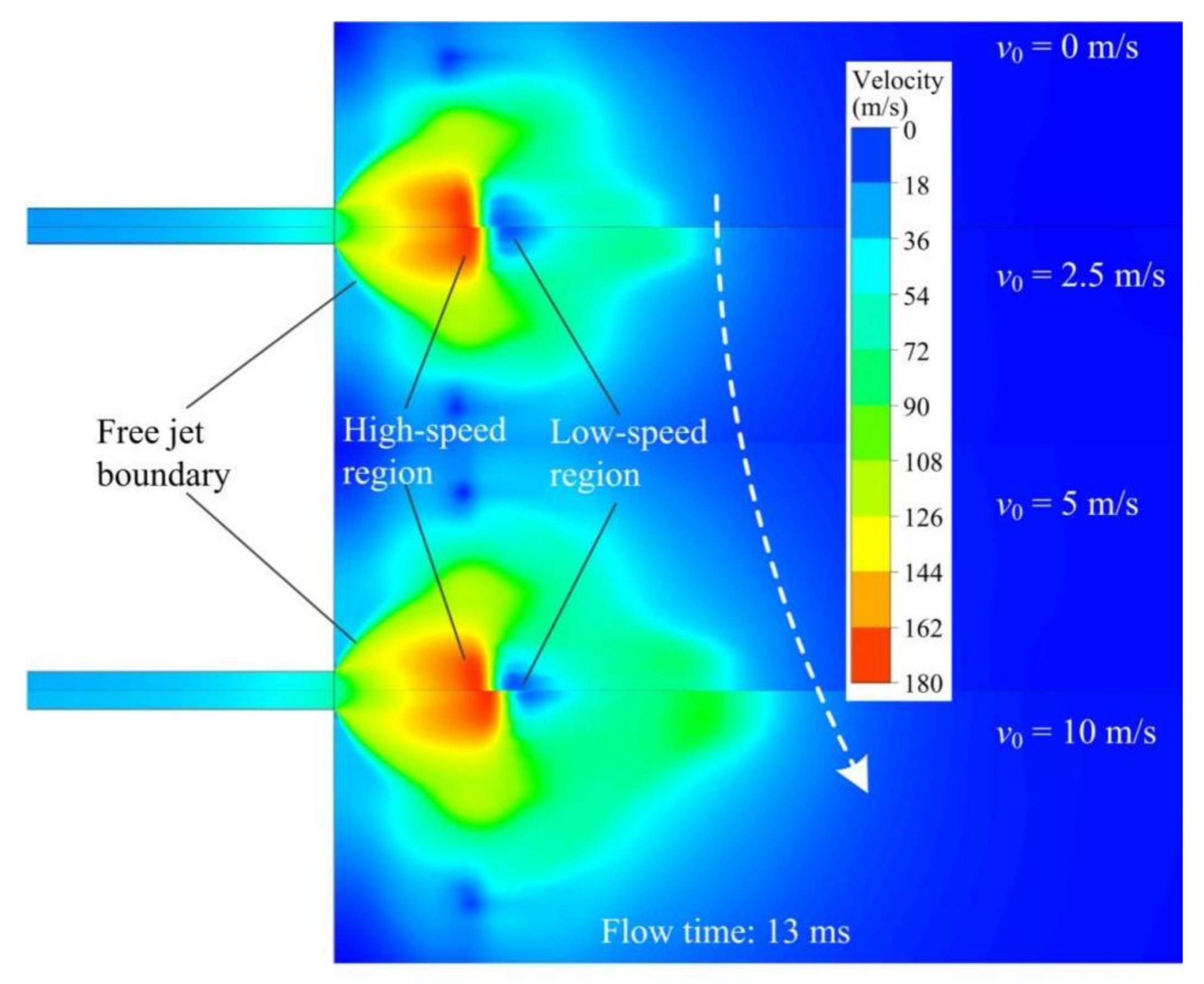
The near-field jet structures around the rupture opening are shown in Figure 12, which mainly includes free jet boundary, a high-speed region and a low-speed region formed by a series of back-propagating compression waves due to the fact that the local pressure was lower than the surrounding pressure. It was found that a larger initial flow velocity accelerated the formation of the near-field jet, that is, the high-speed region was widened while the low-speed region was narrowed. The maximum flow velocity of the high-speed region was only 180 m/s at a flow time of 13 ms. Similar experiments with an inner pressure of 15 MPa (liquid CO2) were carried by Liu [36], the measured maximum velocities of the near-field jets from nozzles with ID of 15 and 20 mm were 104.26 and 114.42 m/s, respectively. The maximum velocities of the near-field jets were much lower than that of the gas jets, the main reason was that the CO2 fluid ejected from the outlet was mainly composed of liquid CO2, which rapidly vaporized into gas CO2 and formed a gas–liquid two-phase flow in atmospheric environment. Compared with gas flow, liquid flow had a higher resistance when injected into the atmosphere. The resistance of gas–liquid two-phase flow, however, was in between them. That is, the expanding velocity of the gas–liquid two-phase flow was lower than that of pure gas flow.
5. Conclusions
In this paper, a CFD decompression model based on the non-equilibrium phase transition and Span–Wagner EoS was developed to investigate the effects of the relaxation time coefficients and initial flow velocity of CO2 on the decompression behaviour within the pipe and the near-field jet out of the rupture opening, as well as the mass flow at the rupture opening. To verify the CFD model, a test of large-scale “shock tube” with an ID of 146.36 mm was simulated. It was found that the evaporation coefficient showed a significant impact on the transition behaviour of CO2 decompression, while the condensation coefficient basically had no effect on it. When the evaporation coefficient was set to be 15 s−1, the CFD prediction results were in good agreement with the test results.
The initial flow velocity had a minor effect on the “pressure plateau” value of CO2 inside pipe, while having a major impact on the temperature drop. The results showed that a smaller initial flow resulted in a faster temperature drop, which made the fluid more prone to phase transition, resulting in a higher volume fraction of gas CO2 phase in the same flow time. In addition, the local outflow velocity increased with an increase in initial flow velocity.
The total mass flow of the rupture opening was directly proportional to the flow velocity. The mass flow rate of gas CO2 increased with the increase in initial flow velocity. Moreover, the mass flows of gas CO2 were all about 20 kg/s at a flow time of 20 ms, and the total mass flows were all above 500 kg/s, which indicated that most of the CO2 fluids leaking from the rupture opening were in a liquid state during decompression.
The initial flow velocity also affected the distribution range of velocity field and volume fraction of gas CO2 outside the opening. The ejected gas–liquid two-phase CO2 flow quickly vaporized into gas CO2, and then about 1% of the gas CO2 condensed into liquid CO2. In addition, the maximum flow velocity of the near-field jet composed of gas CO2 and liquid CO2 was only 180 m/s at a flow time of 13 ms.
Author Contributions
Writing—original draft preparation and methodology, C.X.; supervisition, Z.L.; investigation, L.Y.; software, J.W.; funding acquisition, writing-review and editing, S.Y. All authors have read and agreed to the published version of the manuscript.
Funding
This research was funded by National Youth Foundation of China, grant number 11902369.
Institutional Review Board Statement
Not applicable.
Informed Consent Statement
Not applicable.
Data Availability Statement
The data presented in this study are available on request from the corresponding author.
Acknowledgments
The authors would like to acknowledge the support from the High Speed Train Research Center of Central South University (CSU, China).
Conflicts of Interest
The authors declare no conflict of interest.
References
- Pierre, F.; Matthew, W.J.; Michael, O.’S. Global Carbon Budget. Earth Syst. Sci. Data 2019, 11, 1783–1838. [Google Scholar] [CrossRef] [Green Version]
- Global Monitoring Laboratory (NOAA). Mauna Loa Laboratory CO2 Monitoring Records National Oceanic & Atmospheric Administration. 2020. Available online: https://www.esrl.noaa.gov/gmd/ccgg/trends/ (accessed on 31 May 2020).
- Rockstrom, J.; Steffen, W.; Noone, K.; Persson, A.; Chapin, F.S. A safe operating space for humanity. Nature 2009, 461, 472–475. [Google Scholar] [CrossRef] [PubMed]
- IPCC. IPCC Special Report on Carbon Dioxide Capture and Storage, Repared by Working Group III of the IPCC; Cambridge University Press: Cambridge, UK, 2005. [Google Scholar]
- Sven-Lasse, K.; Martin, P.; Stefan, S.; Alfons, K.; Heike, R. Potential dynamics of CO2 stream composition and mass flow rates in CCS clusters. Processes 2020, 8, 1188. [Google Scholar]
- Forbes, S.M.; Verma, P.; Curry, T.E.; Friedmann, S.J.; Wade, S.M. CCS Guidelines for Carbon Dioxide Capture, Transport, and Storage; World Resources Institute (WRI): Washington, DC, USA, 2008. [Google Scholar]
- Elshahomi, A.; Lu, C.; Michal, G.; Liu, X.; Godbole, A.; Venton, P. Decompression wave speed in CO2 mixtures: CFD modelling with the GERG-2008 equation of state. Appl. Energy 2015, 140, 20–32. [Google Scholar] [CrossRef] [Green Version]
- Wells, A. Fracture control: Past, present and future. Exp. Mech. 1973, 13, 401–410. [Google Scholar] [CrossRef]
- Cosham, A.; Jones, D.G.; Armstrong, K.; Allason, D. Ruptures in gas pipelines, liquid pipelines and dense phase carbon dioxide pipelines. In Proceedings of the 9th International Pipeline Conference, Calgary, AB, Canada, 24–28 September 2012. [Google Scholar]
- Botros, K.K.; Geerligs, J.; Rothwell, B.; Robinson, T. Measurements of decompression wave speed in pure carbon dioxide and comparison with predictions by equation of state. J. Pres. Ves. Technol. 2016, 138, 031302. [Google Scholar] [CrossRef]
- Vree, B.; Ahmad, M.; Buit, L.; Florisson, O. Rapid depressurization of a CO2 pipeline-An experimental study. Int. J. Greenh. Gas Control 2015, 41, 41–49. [Google Scholar] [CrossRef]
- Loi, H.H.P.P.; Risza, R. A review of experimental and modelling methods for accidental release behaviour of high-pressurised CO2 pipelines at atmospheric environment. Process. Saf. Environ. 2016, 104, 48–84. [Google Scholar]
- Guo, X.; Yan, X.; Yu, J.; Yang, Y.; Zhang, Y.; Chen, S.; Mahgerefteh, H.; Martynov, S. Pressure responses and phase transitions during the release of high pressure CO2 from a large-scale pipeline. Energy 2016, 118, 1066–1078. [Google Scholar] [CrossRef] [Green Version]
- Guo, X.; Yan, X.; Yu, J.; Zhang, Y.; Chen, S.; Mahgerefteh, H.; Martynov, S.; Collard, A.; Proust, C. Pressure response and phase transition in supercritical CO2 releases from a large-scale pipeline. Appl. Energy 2016, 178, 189–197. [Google Scholar] [CrossRef]
- Guo, X.; Chen, S.; Yan, X.; Zhang, X.; Yu, J.; Zhang, Y.; Mahgerefteh, H.; Martynov, S.; Collard, A.; Brown, S. Flow characteristics and dispersion during the leakage of high pressure CO2 from an industrial scale pipeline. Int. J. Greenh. Gas Control 2018, 73, 70–78. [Google Scholar] [CrossRef] [Green Version]
- Lu, C.; Elshahomi, A.; Godbole, A.; Rothwell, B. Investigation of the effects of pipe wall roughness and pipe diameter on the decompression wave speed in natural gas pipelines. In Proceedings of the 9th International Pipeline Conference, Calgary, AB, Canada, 24–28 September 2012. [Google Scholar]
- Cosham, A.; Jones, D.G.; Armstrong, K.; Allason, D.; Barnett, J. The decompression behaviour of carbon dioxide in the dense phase. In Proceedings of the 9th International Pipeline Conference, Calgary, AB, Canada, 24–28 September 2012. [Google Scholar]
- Mahgerefteh, H.; Brown, S.; Martynov, S. A study of the effects of friction, heat transfer, and stream impurities on the decompression behavior in CO2 pipelines. Greenh. Gases-Sci. Technol. 2012, 2, 369–379. [Google Scholar] [CrossRef]
- Mahgerefteh, H.; Zhang, P.; Brown, S. Modelling brittle fracture propagation in gas and dense-phase CO2 transportation pipelines. Int. J. Greenh. Gas Control 2016, 46, 39–47. [Google Scholar] [CrossRef]
- Phillips, A.G.; Robinson, C.G. Gas Decompression Behavior Following the Rupture of High Pressure Pipelines—Phase 1 PRCI Contract PR-273-0135; Pipeline Research Council International Inc.: Arlington, VA, USA, 2002; pp. 1–52. [Google Scholar]
- Cosham, A.; Eiber, R.J. Fracture control in carbon dioxide pipelines—Teffect of impurities. In Proceedings of the 7th International pipeline conference, Calgary, AB, Canada, 29 September–3 October 2008; pp. 229–240. [Google Scholar]
- Ramachandran, H.; Pope, G.A.; Srinivasan, S. Numerical study on the effect of thermodynamic phase changes on CO2 leakage. Energy Procedia 2017, 114, 3528–3536. [Google Scholar] [CrossRef]
- Xia, G.; Li, D.; Merkle, C.L. Consistent properties reconstruction on adaptive Cartesian meshes for complex fluids computations. J. Comput. Phys. 2007, 225, 1175–1197. [Google Scholar] [CrossRef]
- Downar-Zapolski, P.; Bilicki, Z.; Bolle, L.; Franco, J. The non-equilibrium relaxation model for one-dimensional flashing liquid flow. Int. J. Multiph. Flow 1996, 22, 473–483. [Google Scholar] [CrossRef]
- Bilicki, Z.; Kestin, J. Physical aspects of the relaxation model in two-phase flow. Proc. R. Soc. Lond. A 1990, 428, 379–397. [Google Scholar]
- Brown, S.; Martynov, S.; Mahgerefteh, H.; Chen, S.; Zhang, Y. Modelling the non-equilibrium two-phase flow during depressurisation of CO2 pipelines. Int. J. Greenh. Gas Control 2014, 30, 9–18. [Google Scholar] [CrossRef] [Green Version]
- Brown, S.; Martynov, S.; Mahgerefteh, H.; Proust, C. A homogeneous relaxation flow model for the full bore rupture of dense phase CO2 pipelines. Int. J. Greenh. Gas Control 2013, 17, 349–356. [Google Scholar] [CrossRef]
- Zheng, W.; Mahgerefteh, H.; Martynov, S.; Brown, S. Modelling of CO2 decompression across the triple point. Ind. Eng. Chem. Res. 2017, 56, 10491–10499. [Google Scholar] [CrossRef]
- Liu, B.; Liu, X.; Lu, C.; Ajit, G.; Guillaume, M.; Anh, K.T. A CFD decompression model for CO2 mixture and the influence of non-equilibrium phase transition. Appl. Energy 2018, 227, 516–524. [Google Scholar] [CrossRef]
- Xiao, C.; Lu, Z.; Yan, L.; Yao, S. Transient behaviour of liquid CO2 decompression: CFD modelling and effects of initial state parameters. Int. J. Greenh. Gas Control 2020, 101, 103154. [Google Scholar] [CrossRef]
- ANSYS. Ansys Fluent Theory Guide; ANSYS Inc.: Canonsburg, PA, USA, 2018. [Google Scholar]
- Lee, W.H. A Pressure Iteration Scheme for Two-Phase Flow Modelling. Multiphase Transport Fundamentals, Reactor Safety, Applications; Hemisphere Publishing: Washington, DC, USA, 1980. [Google Scholar]
- Span, R.; Wagner, W. A new equation of state for carbon dioxide covering the fluid region from the Triple-Point temperature to 1100 K at pressures up to 800 MPa. J. Phys. Chem. Ref. Data 1996, 25, 1509–1596. [Google Scholar] [CrossRef] [Green Version]
- Shih, T.H.; Liou, W.W.; Shabbir, A.; Yang, Z.; Zhu, J. A new k-ε eddy–viscosity model for high reynolds number turbulent flows-model development and validation. Comput. Fluids 1995, 24, 227–238. [Google Scholar] [CrossRef]
- Marta, S.; Marek, J. Multiphase model of flow and separation phases in a whirlpool: Advanced simulation and phenomena visualization approach. J. Food Eng. 2020, 274, 109846. [Google Scholar]
- Liu, Z.; Zhao, Y.; Ren, T.; Qian, X.; Zhou, Y.; Sun, R.; Li, T.; Zhang, D. Experimental study of the flow characteristics and impact of dense–phase CO2 jet releases. Process. Saf. Environ. 2018, 116, 208–218. [Google Scholar] [CrossRef]
Figure 1.
Schematic diagram of (a) computational domain and (b) computational meshes. The meshes around the wall and rupture openings have been refined.
Figure 1.
Schematic diagram of (a) computational domain and (b) computational meshes. The meshes around the wall and rupture openings have been refined.

Figure 2.
Pressure changes obtained using different mesh densities.

Figure 3.
Effects of evaporation coefficient τlv on (a) pressure, (b) mass flow, (c) flow velocity and (d) volume fraction of gas CO2 phase at flow time of 10 ms. The location of 0.0 m is the rupture opening.
Figure 3.
Effects of evaporation coefficient τlv on (a) pressure, (b) mass flow, (c) flow velocity and (d) volume fraction of gas CO2 phase at flow time of 10 ms. The location of 0.0 m is the rupture opening.

Figure 4.
Effects of condensation coefficient τvl on volume fraction of gaseous CO2 phase.

Figure 5.
Comparison of (a) pressure and (b) decompression wave speed (the data points by test were from Cosham [17], and the evaporation coefficient and condensation coefficient were both 15 s−1 in the CFD simulations).
Figure 5.
Comparison of (a) pressure and (b) decompression wave speed (the data points by test were from Cosham [17], and the evaporation coefficient and condensation coefficient were both 15 s−1 in the CFD simulations).

Figure 6.
Effects of flow velocity on (a) pressure and (b) temperature.

Figure 7.
Effects of flow velocity on volume fraction of gas CO2.

Figure 8.
Effects of flow velocity on (a) local outflow velocity and (b) decompression wave speed.

Figure 9.
Effects of flow velocity on (a) total mass flow and (b) mass flow of gas CO2 of rupture opening.
Figure 9.
Effects of flow velocity on (a) total mass flow and (b) mass flow of gas CO2 of rupture opening.

Figure 10.
Effects of flow velocity on (a) total pressure and (b) volume fraction of gas CO2 out of rupture opening (location of 0 m is the rupture opening) at a flow time of 13 ms.
Figure 10.
Effects of flow velocity on (a) total pressure and (b) volume fraction of gas CO2 out of rupture opening (location of 0 m is the rupture opening) at a flow time of 13 ms.

Figure 11.
Volume fraction of gas CO2 with an initial flow velocity of (a) 0 m/s, (b) 2.5 m/s, (c) 5 m/s and (d) 10 m/s. The flow time of the left picture was 5 ms, and the flow time of the right picture was 13 ms.
Figure 11.
Volume fraction of gas CO2 with an initial flow velocity of (a) 0 m/s, (b) 2.5 m/s, (c) 5 m/s and (d) 10 m/s. The flow time of the left picture was 5 ms, and the flow time of the right picture was 13 ms.

Figure 12.
Effects of flow velocity on velocity distribution of near field flow.


Table 1.
Initial computational parameters of cases.
| Cases | P0 (MPa) | T0 (K) | ρ0 (kg/m−3) | v0 (m/s) | τlv (s−1) | τvl (s−1) |
|---|---|---|---|---|---|---|
| 1 | 15.24 | 278.15 | 978.61 | 0.0 | 0.1 | 15.0 |
| 2 | 15.24 | 278.15 | 978.61 | 0.0 | 30.0 | 15.0 |
| 3 | 15.24 | 278.15 | 978.61 | 0.0 | 15.0 | 0.1 |
| 4 | 15.24 | 278.15 | 978.61 | 0.0 | 15.0 | 50.0 |
| 5 | 15.24 | 278.15 | 978.61 | 0.0 | 15.0 | 15.0 |
| 6 | 15.24 | 278.15 | 978.61 | 2.5 | 15.0 | 15.0 |
| 7 | 15.24 | 278.15 | 978.61 | 5.0 | 15.0 | 15.0 |
| 8 | 15.24 | 278.15 | 978.61 | 10.0 | 15.0 | 15.0 |
Publisher’s Note: MDPI stays neutral with regard to jurisdictional claims in published maps and institutional affiliations. |
© 2021 by the authors. Licensee MDPI, Basel, Switzerland. This article is an open access article distributed under the terms and conditions of the Creative Commons Attribution (CC BY) license (http://creativecommons.org/licenses/by/4.0/).
Share and Cite
MDPI and ACS Style
Xiao, C.; Lu, Z.; Yan, L.; Wang, J.; Yao, S. Effects of Flow Velocity on Transient Behaviour of Liquid CO2 Decompression during Pipeline Transportation. Processes 2021, 9, 192. https://doi.org/10.3390/pr9020192
AMA Style
Xiao C, Lu Z, Yan L, Wang J, Yao S. Effects of Flow Velocity on Transient Behaviour of Liquid CO2 Decompression during Pipeline Transportation. Processes. 2021; 9(2):192. https://doi.org/10.3390/pr9020192
Chicago/Turabian StyleXiao, Chenghuan, Zhaijun Lu, Liguo Yan, Jiaqiang Wang, and Shujian Yao. 2021. "Effects of Flow Velocity on Transient Behaviour of Liquid CO2 Decompression during Pipeline Transportation" Processes 9, no. 2: 192. https://doi.org/10.3390/pr9020192
Note that from the first issue of 2016, this journal uses article numbers instead of page numbers. See further details here.