Large Eddy Simulation of Film Cooling Involving Compound Angle Holes: Comparative Study of LES and RANS


School of Mechanical Engineering, Kookmin University, 77 Jeongneung-ro, Seongbuk-gu, Seoul 02707, Korea
*
Author to whom correspondence should be addressed.
Processes 2021, 9(2), 198; https://doi.org/10.3390/pr9020198
Submission received: 28 December 2020
/
Revised: 18 January 2021
/
Accepted: 19 January 2021
/
Published: 21 January 2021
(This article belongs to the Special Issue CFD Applications in Energy Engineering Research and Simulation)
Abstract
:A large eddy simulation (LES) was performed for film cooling in the gas turbine blade involving spanwise injection angles (orientation angles). For a streamwise coolant injection angle (inclination angle) of 35°, the effects of the orientation angle were compared considering a simple angle of 0° and 30°. Two ratios of the coolant to main flow mass flux (blowing ratio) of 0.5 and 1.0 were considered and the experimental conditions of Jung and Lee (2000) were adopted for the geometry and flow conditions. Moreover, a Reynolds averaged Navier–Stokes simulation (RANS) was performed to understand the characteristics of the turbulence models compared to those in the LES and experiments. In the RANS, three turbulence models were compared, namely, the realizable k-ε, k-ω shear stress transport, and Reynolds stress models. The temperature field and flow fields predicted through the RANS were similar to those obtained through the experiment and LES. Nevertheless, at a simple angle, the point at which the counter-rotating vortex pair (CRVP) collided on the wall and rose was different from that in the experiment and LES. Under the compound angle, the point at which the CRVP changed to a single vortex was different from that in the LES. The adiabatic film cooling effectiveness could not be accurately determined through the RANS but was well reflected by the LES, even under the compound angle. The reattachment of the injectant at a blowing ratio of 1.0 was better predicted by the RANS at the compound angle than at the simple angle. The temperature fluctuation was predicted to decrease slightly when the injectant was supplied at a compound angle.
1. Introduction
Gas turbines, which are composed of compressors, combustors, and turbines, are mainly used as aircraft engines and prime movers for natural gas power generation. Ensuring cycle efficiency is critical in both these applications. Although additional devices such as reheaters or regenerators can be installed to increase cycle efficiency, this technique cannot be adopted in the case of aircraft engines due to the limitations of the weight and frontal area. Therefore, in general, to increase cycle efficiency, the turbine inlet temperature is raised above the allowable temperature limit of the materials by cooling the blade through the air from the compressor [1].
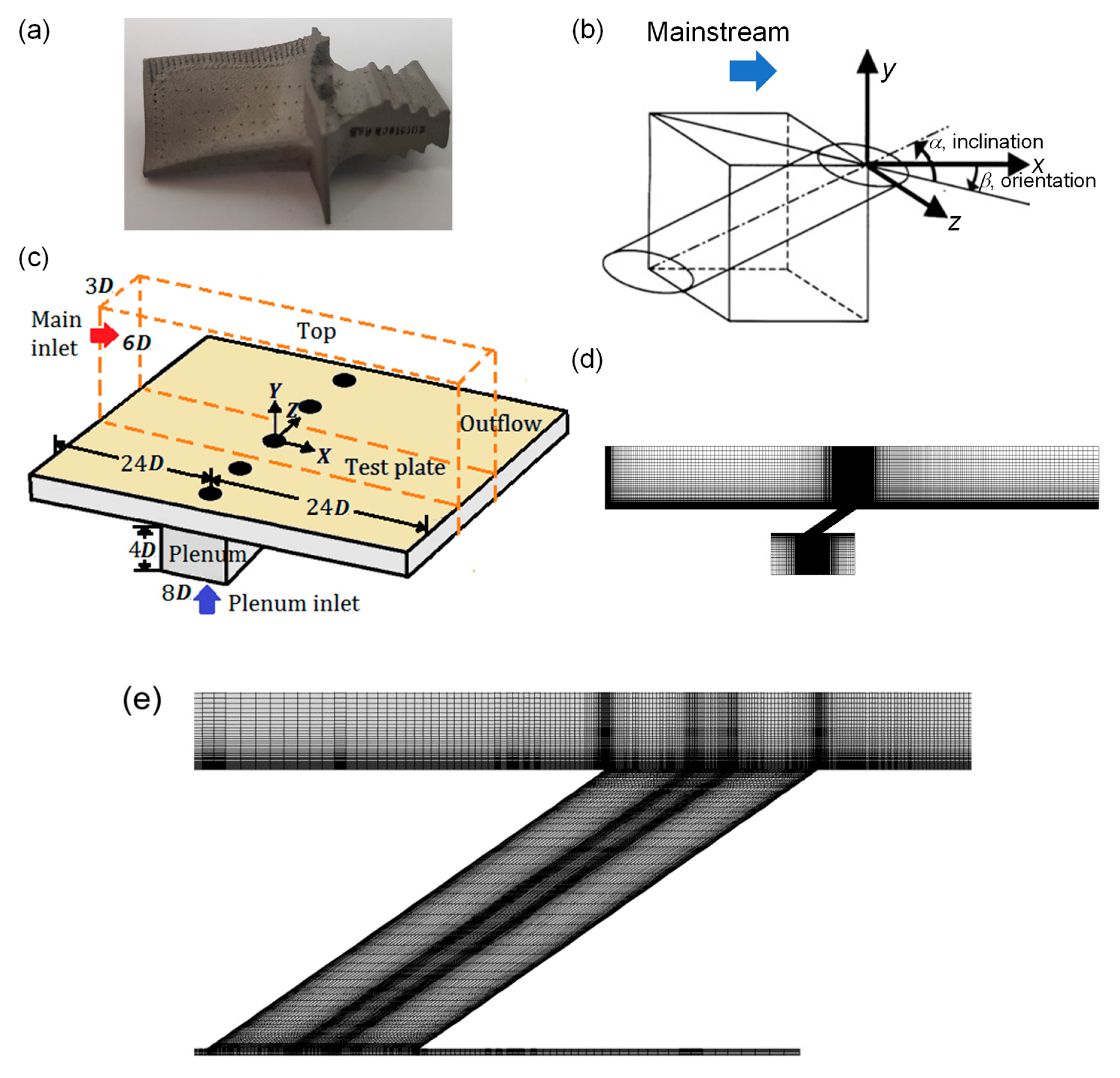
The cooling air extracted from the compressor is supplied to the internal cooling passage of the turbine blade to cool the blade. After cooling the inside of the blade, the air, injected through the blade surface, flows on the surface, thereby creating an insulating film to protect the blade from the hot combustion gases. To generate a uniform insulation film, it is advantageous to inject the coolant through a slot. However, to ensure the mechanical strength, cylindrical holes are usually arrayed in the spanwise direction, as shown in Figure 1a [2].
Over 50 years, numerous experiments and numerical studies have been conducted by many researchers to understand the physics of film cooling. Goldstein, Eckert, and Ramsey obtained the film cooling effectiveness on a flat plate with discrete cylindrical holes, experimentally [3]. They studied the effects of changing Reynolds number for the main flow and the inclination angle of the cooling holes on film cooling effectiveness and concluded that coolant spreading was almost the same regardless of the Reynolds number. They stated that increasing the coolant flow rate made an increase in film cooling effectiveness at low blowing ratios. Pedersen et al. investigated the effects of changing the density ratio of the coolant on film cooling effectiveness experimentally [4]. They also used a flat plate with cylindrical holes and stated that an increasing density ratio resulted in a higher film cooling effectiveness except for the narrow field near the cooling hole due to the coolant jet lifts off and reattachment to the test wall further downstream. Sinha et al. displayed the centerline and spanwise-averaged effectiveness for the various blowing ratios and density ratios experimentally [5]. They showed that increasing the coolant mass flow rate decreased the film cooling effectiveness by the coolant jet lift off. They stated that if the coolant jet to the main flow momentum flux ratio was between 0.3 and 0.7, the coolant jet detachment would occur in the narrow field near the hole and the jets would reattach downstream. If the momentum ratio was more than 0.7, a complete detachment of the coolant jets would be generated. They found that the spanwise-averaged film cooling effectiveness was strongly dependent on the spanwise spreading of the coolant jet.
Owing to structural reasons, the coolant cannot be injected parallel to the surface and is instead injected at an angle to the main flow, with inclination angle α (see Figure 1b) being approximately 30°. In this case, the film cooling jet lifts from the blade surface and interacts with the main flow to generate a counter-rotating vortex pair (CRVP). This flow structure renders the cooling effect uneven and deteriorates the insulation effect owing to the enhanced mixing with the main flow [6,7].
In general, film cooling jets are injected in the streamwise direction to avoid disturbing the main flow however in certain cases, the jets may be injected at a compound angle, with orientation angle β (see Figure 1b) to the main flow. Usually, a compound angle is adopted at the leading edge of the blade to ensure a certain inclination on the curved surface. Moreover, a compound angle is often adopted at the mid-chord to improve the uniformity of the film cooling.
When implementing a compound angle, the film cooling performance changes as the CRVP changes to a single vortex [8,9]. Lee et al. [10] measured the change in the film cooling jet flow for an α value of 35°, with β ranging from 15° to 90°. The CRVP of the film cooling jet exhibited strong asymmetry at an orientation angle of 15° and changed to a single vortex at an orientation angle of 30°. Jung and Lee [11] measured the change in the film cooling effectiveness with the orientation angle. When the compound angle was adopted, film cooling effectiveness increased from 20% to 80% depending on the orientation angle and blowing ratio [11].
Furthermore, flow field information is required to clarify the mechanism of film cooling performance enhancement owing to the compound angle injection or to determine the optimum injection geometry. Lee et al. [10] evaluated the film cooling flow involving a compound angle by using a five-hole Pitot tube however, the measurement did not clarify the turbulent quantities or velocity near the wall. Jung and Lee [11] measured the temperature field, which is a scalar quantity, instead of the velocity vectors. However, the relevant information near the wall was not clarified and the temperature field represents only indirect information regarding the flow field. Abhari et al. [12,13] used the particle image velocimetry (PIV) technique to minimize the disturbance of the flow field pertaining to the sensor and measure the flow field of the film cooling involving a compound angle nevertheless, the velocity near the wall could not be clarified.
The computational fluid dynamics (CFD) technique represents a promising tool to obtain three-dimensional flow field information, including the velocity near the wall. Among the relevant techniques, the most economical approach is the Reynolds averaged Navier–Stokes simulation (RANS), which can accurately reflect the basic flow structures however, the turbulence model cannot effectively predict the mixing of the main flow and film cooling jet, resulting in an overprediction of film cooling effectiveness [14]. The k-ε, k-ω, and Reynolds stress models (RSM) are frequently used in the RANS analysis of film cooling problems. Harrison and Bogard [15] applied the aforementioned three turbulence models and compared the prediction results with the experimentally obtained results. It was noted that the realizable k-ε can best predict the effectiveness of centerline film cooling.
In recent years, film cooling problems were attempted to be solved using the hybrid RANS/large eddy simulation (LES) [16] or the LES [17], which exhibits a higher accuracy but considerably larger computational cost compared to that of the RANS. In the simulation of the film cooling through the hybrid LES or LES, the film cooling effectiveness was better predicted than that in the RANS [16,17]. Moreover, using the instantaneous flow field obtained by the LES, the flow structures that were not visible in the RANS could be identified [18,19,20]. Nevertheless, most of the LES studies on film cooling were based on the use of a simple angle (β = 0°).
The LES results for film cooling involving a compound angle primarily pertained to the case with the leading edge application [21]. Since the leading edge has different film cooling characteristics than those of the mid-chord due to the influence of the pressure gradient and curvature [22,23], it is difficult to directly compare film cooling for simple and compound angle cases by using the data at the leading edge. To clarify the effect of the compound angle injection, the LES for compound angled film cooling applied to a flat plate must be realized.
The LES for a flat plate subjected to a compound angled film cooling was reported [24]. The researchers simulated a two-row film cooling with opposite orientation angles [25]. Nevertheless, the film cooling characteristics with the compound angle could not be identified because the film cooling jets exhibited a unique flow structure due to the strong interaction between the upstream and downstream jets. To determine these characteristics, Li et al. [26] performed an LES for single row compound angle film cooling and clarified the effect of the supply geometry and hole length to diameter ratio (L/D). McClintic et al. [27] studied the effects of internal cross-flow on film cooling effectiveness for a row of cylindrical holes with compound angles of 45° experimentally. They reported that a higher effectiveness was obtained for the cross-flow directed counter to the spanwise direction of the hole than for the cross-flow directed to the spanwise direction of the hole. Stratton et al. [28] investigated the effects of the internal cross-flow on the film cooling performance for a cylindrical hole with a compound angle of 45° by using RANS models and LES. They found that unsteady vortical structures were formed inside the hole and RANS results did not show a good match to an experimental data while LES predicted the film cooling effectiveness with reasonable accuracy.
Overall, although several LES results have been published for the film cooling involving a compound angle on the flat plate geometry, the discussion remains insufficient. The main point of this paper is to show LES results that have remained undiscovered in the past. The flow, thermal fields, and spatial distribution of the film cooling effectiveness obtained by LES and RANS were compared with experimental results. The predictive performance of the three turbulence models for RANS compared for compound angled film cooling, and information regarding the flow and temperature fields near the wall, which could not be determined experimentally, was discussed based on the LES data. In addition, by analyzing the instantaneous flow field obtained from the LES, the flow characteristics of film cooling with a compound angle that could not be determined through the time-averaged analyses, were clarified.
2. Numerical Methods and Validation
2.1. Computational Domain and Boundary Conditions
The computational domain and boundary conditions were set to be comparable with those in the experiments of Jung and Lee [11]. The boundary conditions in the computational domain are specified in Table 1. The domain involved the main flow, test plate, film cooling hole, and plenum, are indicated by the orange box in Figure 1c. The inclination angle of the film cooling jet was 35° and the L/D ratio was 4. The film cooling holes were arranged in a row in the spanwise direction, and the pitch was three times the diameter. The width of the computational domain was set as 3D, according to the pitch and periodic conditions [29,30].
The main flow velocity was 10 m/s and the diameter of the film cooling hole was 1.5 cm. In the experiment of Jung and Lee [11], the flow at the exit of the film cooling hole was a turbulent boundary layer flow and the boundary layer thickness was almost 24 mm (1.6 D). In the CFD simulation, the velocity profile was set to be the same with the experiment. The length of the inlet section was determined as 24 D to ensure that the boundary layer, as in the experiment, was generated at the exit of the hole. To obtain a result not influenced by the boundary conditions up to x/D = 15, which corresponded to the film cooling effectiveness distribution in the work of Jung and Lee [11], the size of the computational domain downstream of the hole was set as 24 D and the pressure outlet conditions were imposed. In LES calculation, the vortex method was adopted at the main inlet and a fluctuation was added on a mean velocity profile by a perturbation of the vorticity field. The vortex points were convected randomly and the vortex method was based on the Lagrangian form of the evolution equation of the vorticity and the Biot–Savart law [31]. On the other hand, in RANS simulation, the turbulent intensity and turbulent length scale were set as 0.2% and 0.1 × height of the inlet, respectively. The turbulent intensity at the main inlet was set as the same in the experiment operating condition.
Simulations were performed considering two blowing ratios of 0.5 and 1.0. In the work of Jung and Lee [11], the film cooling jet penetrated from a high blowing ratio of 1.0 to y/D = 2.0 thus, in this work, the height of the computational domain in the wall-normal direction was determined to be 6 D. Symmetric conditions were imposed on the top surface of the computational domain [29,30]. As shown in Figure 1c, the flow separation occurring at the hole entrance and the interaction of the main flow and injectant at the hole exit were reflected by including the film cooling hole and plenum in the computational domain. The velocity boundary condition at the plenum entrance was imposed to satisfy the blowing ratio requirements.
Jung and Lee [11] compared four orientation angles of 0°, 30°, 60°, and 90°. The experimental apparatus involved five film cooling holes in a row and side walls were present in the test duct. Therefore, in the case of large orientation angles (i.e., 60° and 90°), complete periodicity did not appear in the spanwise direction. Correspondingly, in this study, the simulation cases were considered as those pertaining to 0° (simple angle) and 30°, in which the periodic distribution in the spanwise direction was well reflected in the experimental data.
In terms of the temperature boundary conditions, as in the experiment, the temperature of the main flow and film cooling jet was set as 293 K and 313 K, respectively. A no-slip condition was imposed as the velocity boundary condition on all the walls. Moreover, adiabatic conditions were considered, as in the experiment, to ensure that the adiabatic film cooling effectiveness could be obtained from the surface temperature of the test plate.
The grid system was composed of 2.56 million hexahedrons, based on the results of a sensitivity test. In the streamwise direction, the mesh spacing values range from 6 near the cooling hole to 35 near the end of the domain in x+ units. In the spanwise direction, the mesh spacing values are about 20 throughout the domain in z+ units. As shown in Figure 1d, a non-uniform grid, in which the grid was concentrated near the wall, was used, and 25 grids were stacked within y+ = 30 on the wall and the value of y+ of the first cell above the wall was set as about 1. Figure 1e illustrates the close-up of the mesh near the injection region of the hole.
2.2. Governing Equations and Turbulence Models
The CFD calculations were performed in ANSYS Fluent v. 19, and the meshes were generated in Pointwise v. 18, as shown in Figure 1d [29,30]. Fluent was based on cell-centered finite volume method and the whole computational domain was discretized into a finite number of control volumes. Pointwise was a commercial mesh generation software and structured, unstructured, and hybrid meshes were generated with precise control over points placement. The governing equations included the incompressible Navier–Stokes equation and energy equation. The numerical method used for the cases are a simple scheme. The convection term is solved via second order upwind while the diffusion term is solved by central differencing. In the LES, the governing equation was transformed to a grid filtered equation, as follows [31].
Conservation of Mass (Continuity equation):
Conservation of Momentum:
Conservation of Energy:
In the equations, the overbar represents the grid filtered values. In Equation (2), τij, the subgrid-scale stress was modeled using the Boussinesq hypothesis:
where μt is the subgrid-scale viscosity. The Smagorinsky–Lilly model was adopted based on a validation test [29,30]:
Subgrid-scale viscosity in the Smagorinsky-Lilly model:
In 1877, Boussinesq stated that the momentum transfer generated by turbulent eddies could be modeled with the eddy viscosity. In Equation (3), qj refers to the subgrid-scale heat flux and can be expressed as follows by introducing the subgrid-scale diffusivity αt.
Subgrid-scale heat flux:
μt was considered as αt, assuming that the subgrid-scale turbulent Prandtl number is unity [31].
In the LES, the time step was fixed as 6.25 × 10⁻⁶ s, and the number of steps was 400 considering that the mainstream flowed as much as the hole diameter in this time interval. The film cooling flow is inherently unsteady and the current study performed the statistically steady state analysis by post-processing. A total of 20,000 time steps were required from the initial condition to reach steady state and 30,000 integrated time steps were considered to obtain the average flow field and statistics. The complete process required approximately one month of computation time on a 20-core-cluster computer. The RANS analyzed the time-averaged continuity, Navier–Stokes, and energy equations, as shown in Equations (7)–(9), respectively.
Conservation of Mass (Continuity equation):
Conservation of Momentum:
Conservation of Energy:
Six turbulent stress components, ,, , , , and from Equation (8) and three turbulent heat flux components , , and from Equation (9) were required to be modeled. The RSM, realizable k-ε model, and k-ω shear stress transport (SST) model were compared. Detailed equations for each of these models can be found elsewhere, such as the work of Tannehill et al. [32]. The RANS computations converged to the 10−6 level for all the equations in approximately 10 h on a 20-core-cluster computer.
2.3. Code Validation
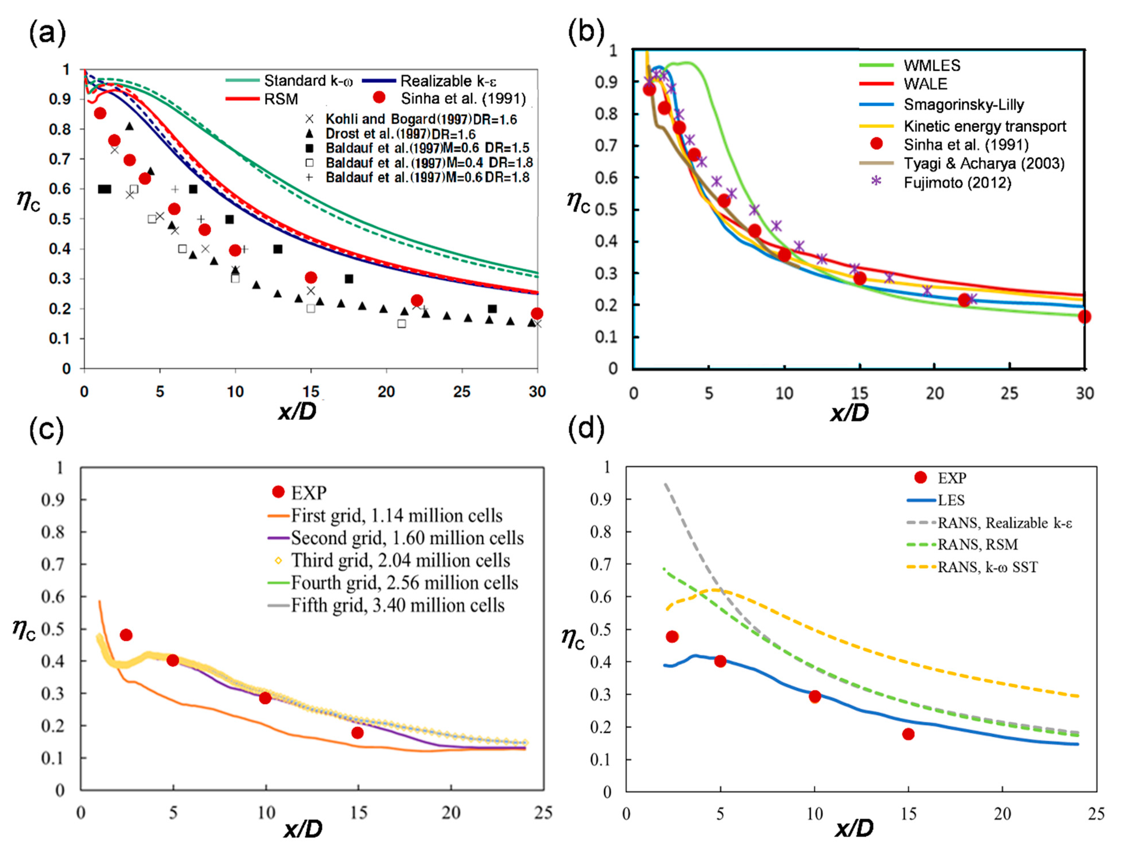
Harrison and Bogard [15] performed a RANS by using three models and as shown in Figure 2a, the centerline film cooling effectiveness prediction of the realizable k-ε and RSM models was more accurate than that of the k-ω. Considering the experimental conditions adopted by Sinha et al. [5], the LES was performed on four subgrid-scale models, as shown in Figure 2b and the findings were compared with two sets of LES data in the open literature [17,33]. The LES results for the effectiveness corresponded to a higher correlation with the experimental data than the RANS data, as shown in Figure 2a.
Among the subgrid-scale models, the predictions of the wall adapting local eddy-viscosity model, Smagorinsky–Lilly model, and kinetic energy transport model (excluding those of the wall modeled LES) were equivalently correlated with the experimental values. WMLES (Wall-Modeled Large Eddy Simulation) and WALE (Wall-Adapting Local Eddy-Viscosity) models did not show a good match with the experimental data in the near-hole region and in the far field region, respectively. Considering these findings, the Smagorinsky–Lilly model was adopted in the present study.
Subsequently, a grid sensitivity test was conducted through the LES under the geometry and flow conditions considered by Jung and Lee [11] to compare the data in this study (see Figure 2c). The comparison for the centerline effectiveness at a blowing ratio of 0.5 indicated that similar results were obtained after 2 million grids. The results obtained using 2.56 million and 3.4 million grid points were completely collapsed and the series of simulations in the present study was thus performed using 2.56 million cells. A series of RANS for film cooling was performed using the three turbulence models in the grid system that passed the grid sensitivity test. As shown in Figure 2d, the RANS data overpredicted the overall film cooling effectiveness compared to those of the LES. For the downstream region after x/D = 7, similar characteristics to those reported by Harrison and Bogard [15] were obtained, as shown in Figure 2a. In other words, the film cooling effectiveness predictions of the realizable k-ε and RSM were equivalent and satisfactory, whereas the k-ω SST overpredicts the effectiveness. For the upstream region with x/D less than 5, the predictions of the RSM and k-ω SST were similar, whereas the realizable k-ε considerably overpredicted film cooling effectiveness.
3. Results and Discussion
3.1. Time-Averaged Flow and Thermal Fields
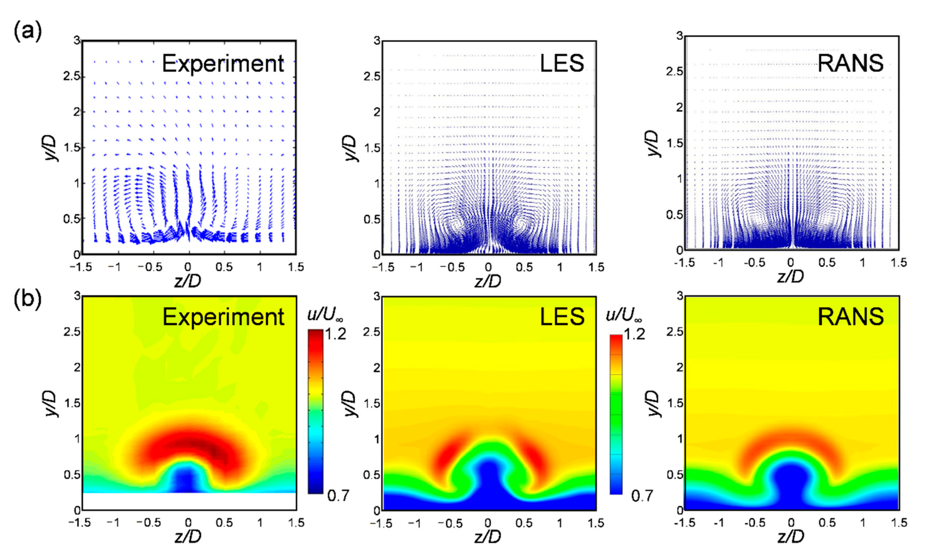
The time-averaged flow and thermal fields obtained by the LES and RANS in a streamwise normal plane were compared with the experimental data of Burd et al. [34] and Jung and Lee [11]. As shown in Figure 2, the film cooling effectiveness differed considerably with the turbulence model however, no significant difference was observed between the time-averaged flow and thermal fields. Therefore, the results of the RANS with the realizable k-ε model were compared with those of the experiments and LES as a representative case. When the orientation angle was 0°, a kidney vortex occurred symmetrically in the film cooling jet and both the LES and RANS predict this phenomenon well, as shown in Figure 3a.
The flow near the wall, which affected the heat transfer characteristics, indicated that the flow of the CRVP created a parallel flow moving along the wall. The two parallel flows collided at the symmetric plane z/D = 0, and rose above the wall. In the experiment, the upward motion started to occur at approximately z/D = 0.5, and the LES predicted this phenomenon well. In the RANS, the v component was observed from approximately z/D = 0.2, closer to the plane of symmetry than in the experimental data. In terms of the streamwise velocity distributions, as shown in Figure 3b, both the LES and RANS exhibited distributions that were similar to the experimental data. Considering the central part of the film cooling jet (z/D = 0, y/D = 0.4) with a dimensionless velocity of 0.7 or less, indicated in blue, it can be noted that the area for the LES data is similar to that of the experiment however, the corresponding area for the RANS data is slightly larger, likely because the RANS predicts that the film cooling jet blocks the main flow more strongly than it actually does. According to the high-speed region marked in red, the LES prediction of the characteristics of the high velocity in the streamwise direction from the kidney vortex position is more similar to the experiment values than those obtained using the RANS.
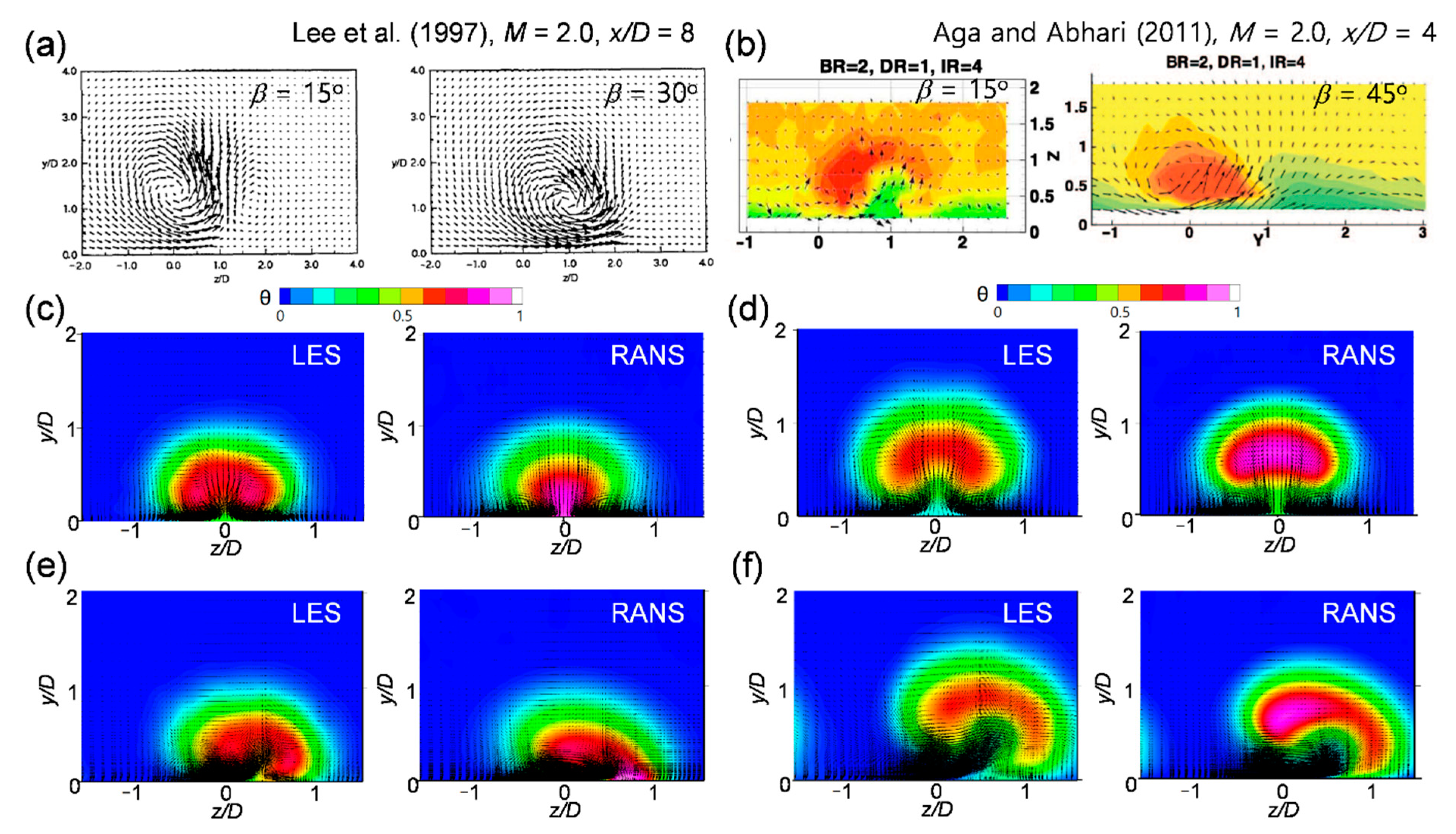
The CFD data provided the velocity information below y/D = 0.2, which could not be measured experimentally. Both the LES and RANS results indicated that the largest and smallest boundary layer thickness occurred at z/D = 0, the plane of symmetry, and at approximately z/D = 0.5, respectively. Therefore, the maximum heat transfer coefficient was expected to occur at approximately z/D = 0.5. The maximum film cooling effectiveness was expected to occur on the plane of symmetry without a strong jet lift-off and this aspect could be confirmed considering the data presented in the next section. Figure 4 shows the structure of the vortex generated in the injectant in a streamwise normal plane in comparison with the experimental data. Since the orientation angle considered in the results shown in Figure 3 was 0°, a left and symmetrical vortex pair appeared. In contrast, when the compound angle was adopted, an asymmetric or single vortex flow occurred. The results obtained using a five-hole Pitot tube [10] (Figure 4a) or PIV [12,13] (Figure 4b) indicated that when the orientation angle was 15°, the counter-rotating vortex remained weak. For the orientation angle of 30° or 45°, the vortex became a single vortex. The particle image velocimetry (PIV) technique minimized the disturbance of the flow field pertaining to the sensor, however, the velocity near the wall could not be clarified because of the measurement method and its limitations.
For the simple angle at a blowing ratio of 0.5 (Figure 4c), the CRVP was observed in both LES and RANS data, and the lift-off of the jet was predicted to a similar degree. Compared to the LES data, the upward flow predicted using the RANS was closer to the symmetry plane, the central temperature was higher, and the hot area marked in red was narrower. When the injection ratio reached 1.0 (Figure 4d), the prediction of the lift-off of the jet of the LES was larger than that of the RANS. In addition, the LES results clearly indicate that the high-temperature region becomes mushroom-shaped owing to the influence of the CRVP.
When the compound angle was adopted, the flow patterns predicted through the LES and RANS at the blowing ratio of 0.5 (Figure 4e) were different. In the LES result, the counter-rotating vortex remained weak however, in the RANS, the vortex changed to a single vortex. The point at which the upward flow started was predicted to be near z/D = 0 and z/D = 0.4 by the LES and RANS, respectively. Lee et al. [10] reported that the CRVP changed to a single vortex at the orientation angle of 30° or more for a single jet. However, for the considered array jet, the transition to a single vortex was delayed at a low blowing ratio.
At a blowing ratio of 1.0 with the compound angle (Figure 4f), the CRVP transformed to a single vortex. The main flow was entrained along the upward flow of the vortex and the hot region was crescent-like. This aspect was common between the LES and RANS however, the LES predicted a higher lift-off than that pertaining to the RANS and the starting point of the upward flow was predicted to be closer to the plane of symmetry.
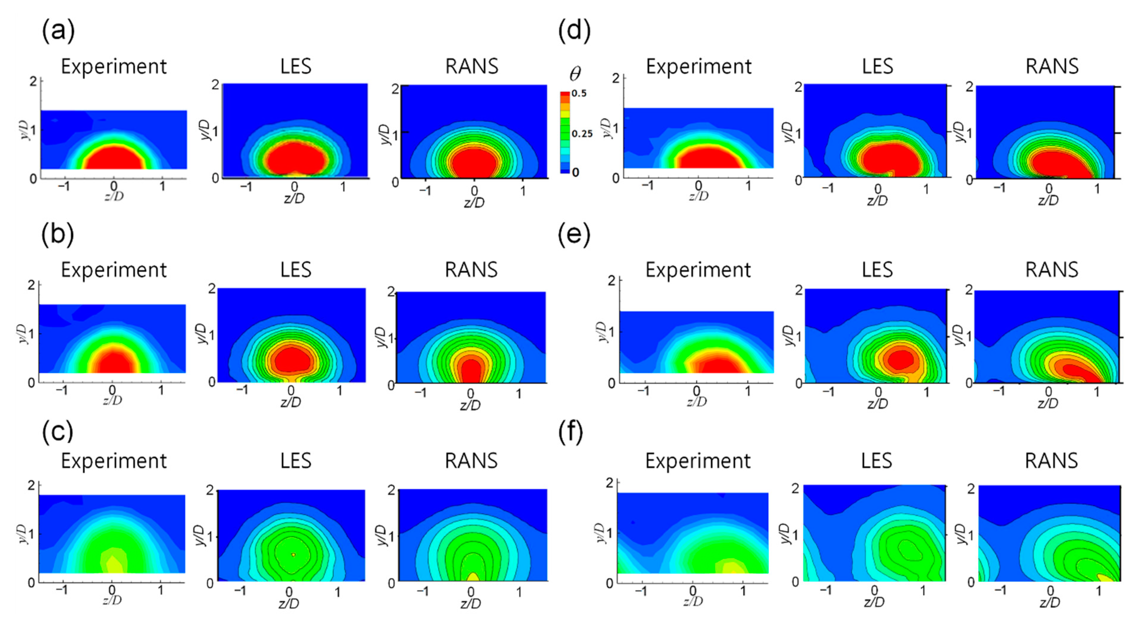
Figure 5 shows a comparison of the boundary layer temperature obtained through the CFD techniques at a blowing ratio of 0.5 with the experimental data presented by Jung and Lee [11] at three streamwise positions. At x/D = 2.5 with a simple angle (Figure 5a), the area of the high-temperature region (displayed in red) predicted by the LES was more similar to the experiment value. The RANS-predicted high-temperature region with a dimensionless temperature θ of 0.5 or higher was smaller than that in the experiment. Even at the downstream position, x/D = 5.0 (Figure 5b), the RANS underpredicted the intensity of mixing with the main flow compared to that obtained in the LES.
In the experimental data, the lift-off was unclear at the upstream locations (Figure 5a,b) because no data near the wall could be obtained through the cold wire measurement. At x/D = 10, as shown in Figure 5c, the center of the injectant appeared near y/D = 0.5 and lift-off could be observed in this part. The LES predicted that the lift-off occurred more intensely than that in the experiment, whereas the RANS did not predict any lift-off.
When the compound angle was adopted, the thermal field became asymmetric. This change in the temperature distribution was well predicted by both the LES and RANS (Figure 5d,f). However, in the case of the compound angle, the mixing characteristics could not be determined simply by considering the area of the hot part, as in the case of the simple angle. Nevertheless, the characteristics could be clarified considering the spacing of the isotherms. In particular, the isotherm spacing in the RANS was wider than that in the experiment.
At a blowing ratio of 0.5, the LES predicted a lift-off and the RANS did not. At x/D = 5.0 (Figure 5b), the point at which the highest temperature occurred was measured to be y/D = 0.3, and the LES predicted the point as y/D = 0.5. The RANS predicted that the highest temperature would occur near the wall even in the downstream location, x/D = 10.
When the blowing ratio reached 1.0, lift-off of the injectant occurred in the case of both the simple and compound angle injection (Figure 6). In Figure 6a, which shows the temperature distribution at x/D = 2.5 for the simple angle, the area marked in red, pertaining to the CRVP, appeared to have an inverted heart shape. As shown in Figure 3, the LES predicted the location of the upward flow near the wall, closer to that in the experiment, and the shape of the high-temperature region obtained using the LES was similar to that in the experiment as well.
As the film cooling jet flowed downstream, it mixed with the main flow, thereby reducing the dimensionless temperature and changing the shape of the temperature distribution. In the case of a simple angle injection, the isotherm shape became similar to a concentric circle as the jet flowed downstream and both the LES and RANS predicted this phenomenon (Figure 6b,c). At x/D = 10 (Figure 6c), the maximum dimensionless temperature was approximately 0.4, observed at a height of approximately y/D = 1, and both the LES and RANS predicted this phenomenon to a similar extent.
In the case of the compound angle, at a blowing ratio of 1.0, the CRVP changed to a single vortex, and the high-temperature region exhibited a crescent shape at x/D = 2.5 (Figure 6d). In the case of the compound angle injection, the LES predicted the lift-off of the injectant to be 10% higher than that in the experimental data, whereas the RANS prediction was similar to the experiment value. The temperature distributions at the downstream locations for the RANS data were more similar to the experiment than those in the LES (Figure 6e,f).
3.2. Adiabatic Film Cooling Effectiveness
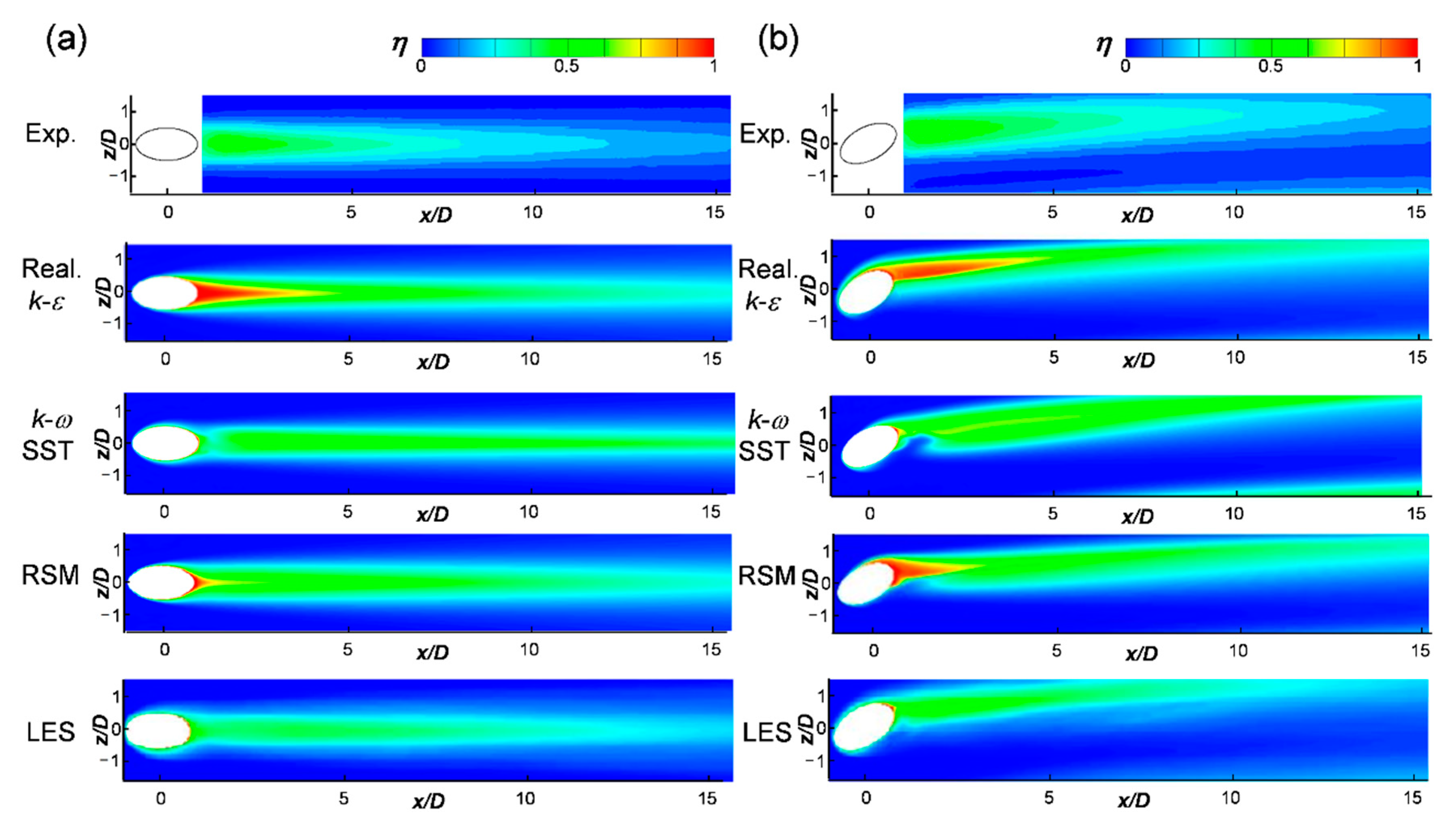
For the local distributions of the adiabatic cooling effectiveness, the LES data and RANS results obtained using three turbulence models were compared with the experimental data presented by Jung and Lee [11]. Figure 7 shows comparisons of the distributions at a blowing ratio of 0.5. In the case of both the simple and compound angles, the LES-obtained distribution was closer to that obtained experimentally than that of the RANS. In the upstream region within x/D = 2, the realizable k-ε and RSM overpredicted the film cooling performance and thus a region with high effectiveness (red contour) appeared, which did not appear in the experimental data. The k-ω SST did not severely overpredict the film cooling effectiveness in the upstream region however, the diffusion in the downstream, compared with the other models, was predicted to be smaller than the experiment value.
In the simple angle case (Figure 7a), the CFD techniques predicted that the film cooling lasted longer than that in the experiment in the downstream region after x/D = 10. Moreover, the CFD results indicated that the spread of the film cooling effect between the holes was delayed downstream compared to that in the experiment. This phenomenon likely occurred because of the influence of the smaller prediction of the CFD for the mixing of the main flow and injectant and the inability to impose artificial perfect insulation similar to that in the CFD in the experiments. By observing the film cooling effectiveness around the hole, which could not be obtained experimentally, the effectiveness around the rim could be attributed to the presence of the horseshoe vortex clearly highlighted in the LES.
In the case of the compound angle (Figure 7b), the region with a high film cooling effectiveness spread widely and alleviated the degradation in the film cooling performance during the downstream flow. These characteristics were better predicted by the LES than by the RANS. The k-ω SST and RSM predicted that a region with low film cooling effectiveness would occur as the main flow was introduced to the surface with the downward flow of the main vortex generated in the film cooling jet in the downstream near the hole. This phenomenon was only slightly reflected in the LES and experiment. Khojasteh et al. [35] reported that the reattachment of the cooling jet occurred at approximately x/D = 1.5 in the simple angle case. Although this phenomenon was not clearly visible at M = 0.5, it could be noted in the experimental results for M = 1.0, as shown in Figure 8.
Reattachment occurred in both the simple and compound angle cases and was more evident in the simple angle case. In the case of the simple angle, the area with high film cooling effectiveness due to the reattachment of the injectant could be observed only in the LES among the CFD results (Figure 8a). The RANS results indicated that the film cooling effectiveness increased after x/D = 5 however, this phenomenon was likely the effect of diffusion by mixing with the main flow rather than the reattachment. As shown in Figure 6, after x/D = 2.5, the height of the center of the injectant did not decrease even when the injectant moved downstream. In the case of the composite angle, both the LES and RANS predicted the occurrence of reattachment. Among the turbulence models, the realizable k-ε model obtained the distribution most similar to that in the experiment. At the blowing ratio of 1.0, the CFD techniques predicted film cooling effectiveness to be lower than that in the experiment and consequently, the distribution shown in Figure 8 involves more blue regions. Overall, the difference in the experimental data and simulation results was greater for the compound angle than for the simple angle.
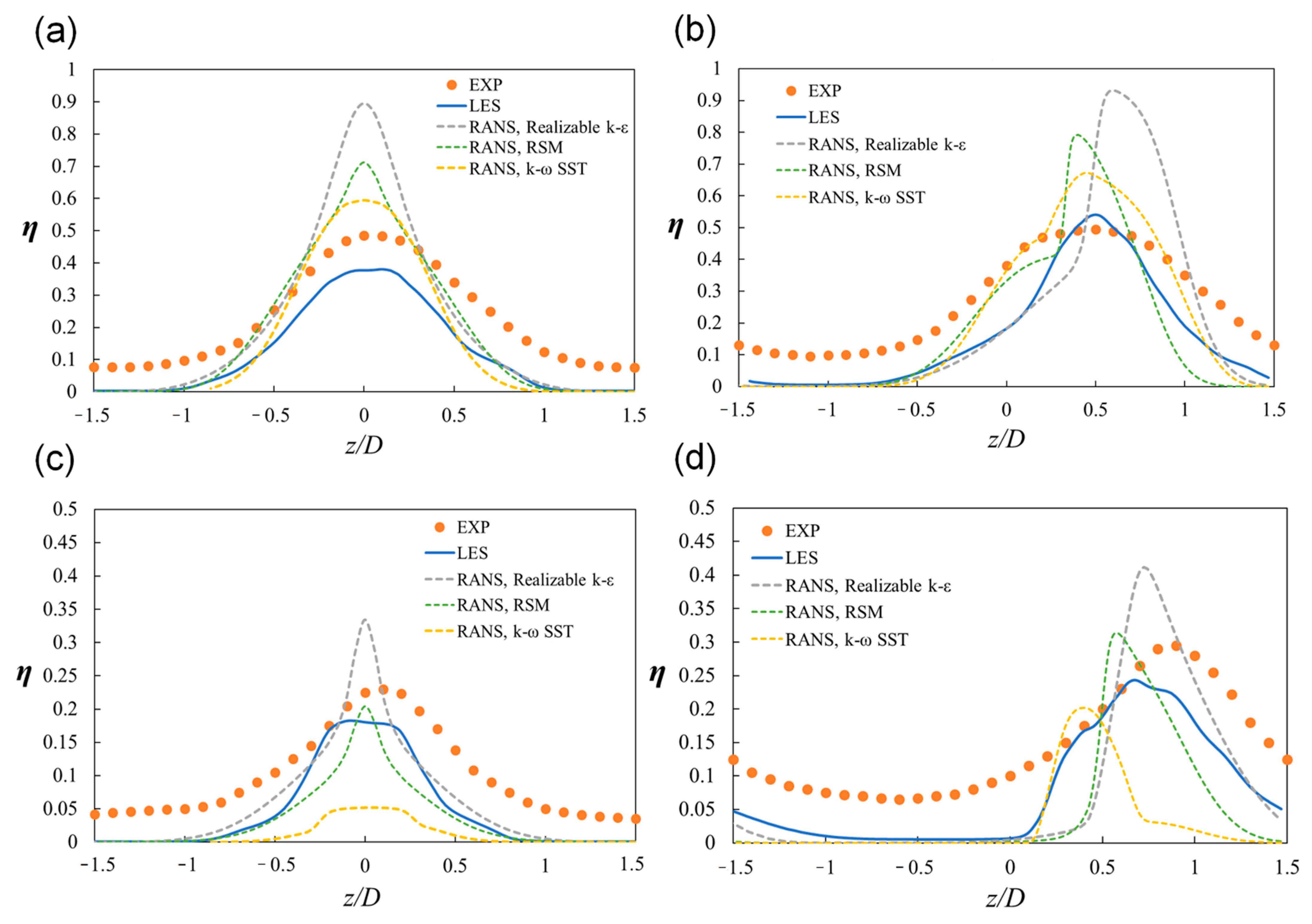
To examine the film cooling performance between the holes and film cooling characteristics in the spanwise direction in the composite angle case, Figure 9 shows the spanwise variation of the film cooling effectiveness at x/D = 2.5. The LES predicted the spanwise diffusion of the film cooling effectiveness better than the RANS. When the blowing ratio increased (Figure 9c,d), the CFD techniques could not predict the spanwise spread accurately. Among the turbulence models, the k-ω SST and RSM obtained the best predictions for the film cooling performance at the blowing ratio of 0.5 and 1.0, respectively. In the case of the simple angle, the realizable k-ε and RSM could not predict the lift-off, and therefore, the centerline film cooling effectiveness was severely overestimated immediately downstream of the hole. The k-ω SST predicted the lift-off well at M = 0.5, albeit incorrectly at M = 1.0, corresponding to the largest difference from the experimental values. All the turbulence models predicted the lift-off more effectively in the case of the composite angle injection than the simple angle injection cases.
3.3. Turbulence Statistics and Instantaneous Flow Fields
Figure 10 shows the turbulence intensity for each component obtained by the LES, in comparison with the experiment of Burd et al. [34]. As the RANS severely underpredicted the turbulence intensity, the maximum values of all the components for the three models did not exceed 10% and thus did not appear within the contour range in Figure 10. In the simple injection angle (β = 0°) case, at M = 1.0, the LES-obtained distribution was similar to that in the experiment under the same geometry and blowing ratio. Compared with that in Figure 3, the turbulence intensity of all the components was high in the part in which upward flow occurred in the CRVP.
The three components exhibit a difference in the turbulence intensity below y/D = 0.2, which could not be measured experimentally. The urms and wrms components not blocked by the wall appeared high along the wall, whereas the vrms component converged to zero at the wall. In the case of the compound angle (β = 30°), the overall trend was similar to that of the simple angle. However, the CRVP changed to a single vortex and consequently, the contours became asymmetric, and the distribution moved in the +z direction.
At the blowing ratio of 0.5, the overall distributions appeared to be smaller than those at M = 1.0 (Figure 10d,f). Under the orientation angle of 30°, the movement in the z direction was smaller than that at the blowing ratio of 1.0. The urms component was larger than that when the blowing ratio was 1.0 near the wall.
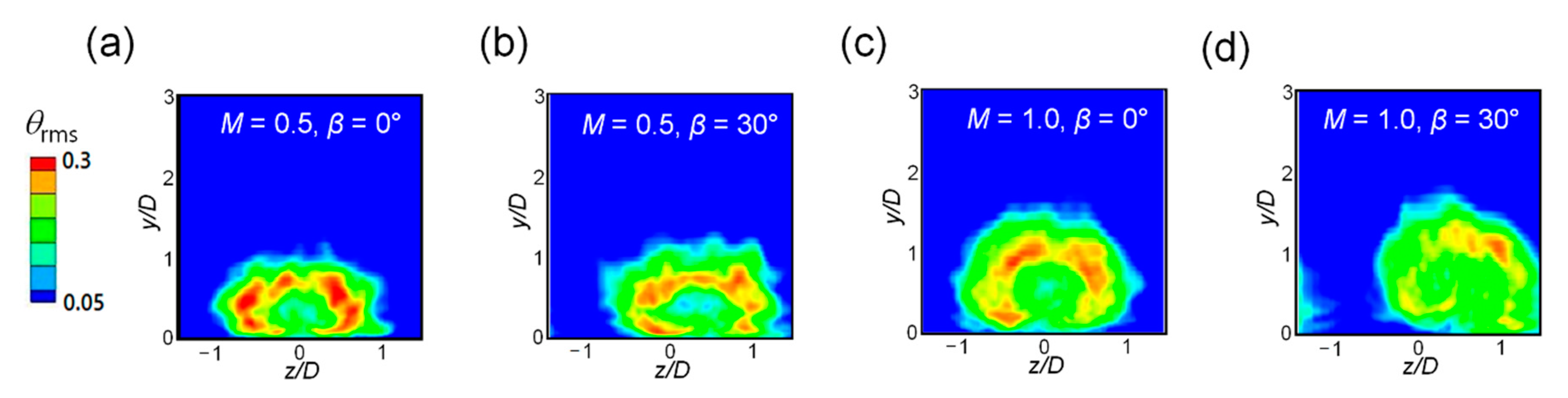
Figure 11 shows the temperature fluctuations. The RANS predicted extremely small temperature fluctuations to be fitted within the contour range, and thus, only the LES results are shown in the figure. θrms was large in the region surrounding the area with large velocity fluctuation, as shown in Figure 10. In the same range of the contours, when β = 0°, the value was slightly higher than that when β = 30°. This finding supports the result of the high film cooling effectiveness under a compound angle as the injectant flowed downstream.
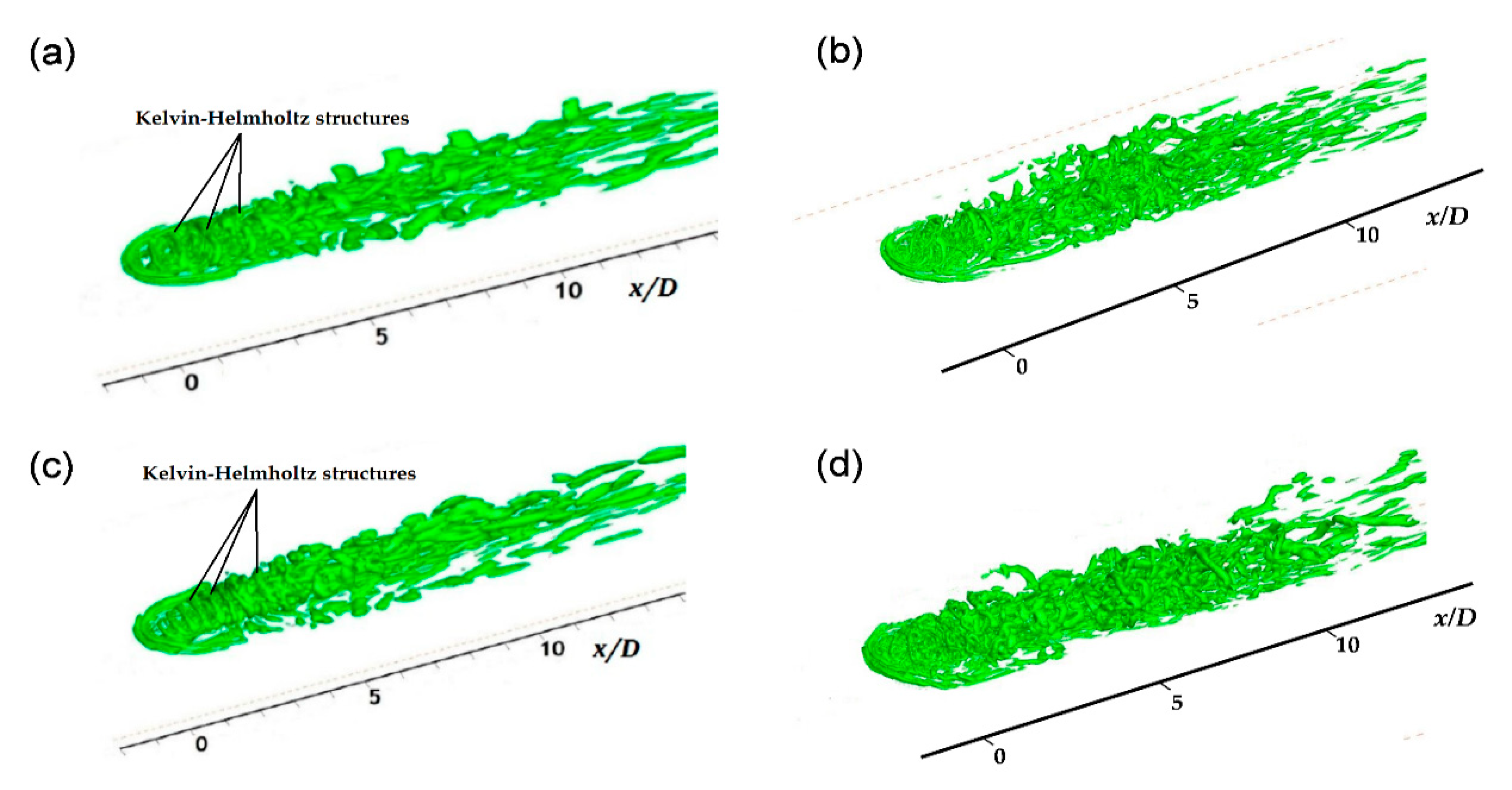
Figure 12 shows the isosurface of the second invariant of the velocity gradient tensor, which is known to reflect the vortex [36]. A horseshoe vortex, Kelvin–Helmholtz vortex, hanging vortex, rear vortex, and hairpin vortex could be observed in all the cases. The CRVP could be observed in the simple angle case, and at the blowing ratio of 1.0 (Figure 12c), the Kelvin-Helmholtz vortex appeared to be stronger with narrow intervals than that at the blowing ratio of 0.5 (Figure 12a).
In the case of the compound angle (Figure 12b,d), the horseshoe vortex became asymmetric and the intensity of the Kelvin–Helmholtz vortex weakened. A single vortex was observed, with more complex vortices generated on the windward side. The vortical structures between the blowing ratios of 0.5 and 1.0 did not exhibit a distinct difference, and at the blowing ratio of 1.0, the injectant moved further in the spanwise direction.
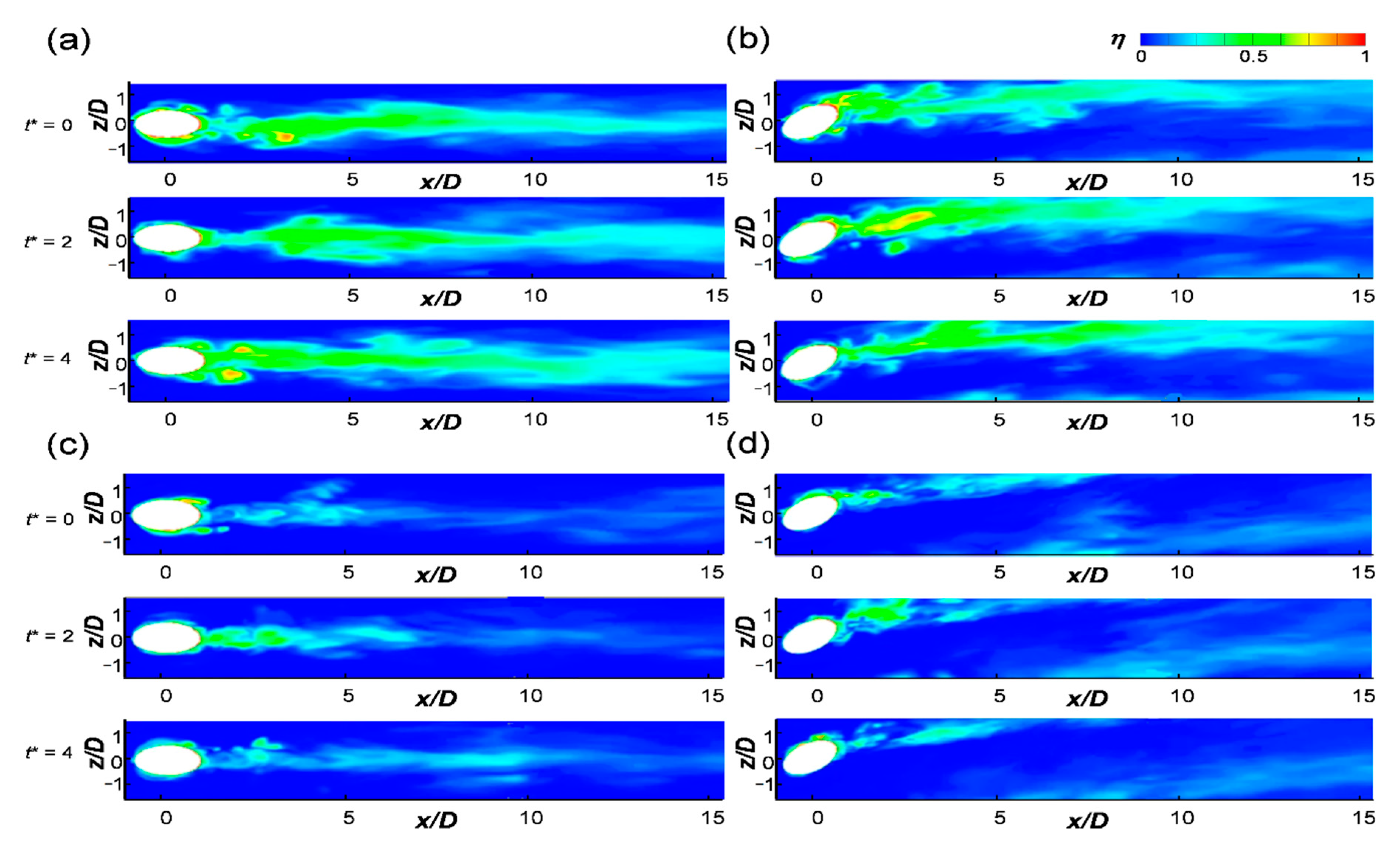
Figure 13 shows the instantaneous temperature field at the wall obtained through the LES. t* is the dimensionless time defined by the main flow velocity and diameter of the hole, such that t* = 1 is the time that the main flow covers a distance equivalent to the hole diameter.
As the adiabatic condition was imposed on the wall, the instantaneous temperature field exhibited the instantaneous adiabatic film cooling effectiveness. When the blowing ratio was 0.5, the injectant flowed along the wall and traces of the injectant, indicated in light green on the contour, extended from the hole to the downstream region (Figure 13a,b). When the blowing ratio reached 1.0, lift-off and reattachment occurred intermittently. As shown in Figure 13c, when t* = 2, traces of the injectant appeared from the hole however, when t* = 4, the traces were eliminated owing to the influence of the near wall vortices, such as the rear vortex shown in Figure 12.
In the case of the simple angle (Figure 13a,c), the film cooling appeared around the rim of the hole due to the influence of the horseshoe vortex and hanging vortex. Under a compound angle, the film cooling effectiveness was reduced around the leeward side of the rim (Figure 13b) or eliminated (Figure 13d). This phenomenon was attributed to the main flow being entrained in the shear layer sweeps while the CRVP changed to a single vortex. In the case of the simple angle injection at the blowing ratio of 1.0, most of the insulating film was eliminated after x/D = 10 (Figure 13c) however, in the case of the compound injection angle, the injectant flowed along the wall and maintained the insulating film (Figure 13d).
4. Conclusions
LES was performed for film cooling with simple and complex angles. Moreover RANS, with three turbulence models, namely, the realizable k-ε, k-ω SST, and RSM, was performed and the spatial distributions of the flow and temperature fields were compared with the experimental data presented at a high resolution. Certain information that was not well predicted with the RANS was clarified and the information that could not be measured experimentally was observed in the LES results. The following conclusions were derived:
- In the time-averaged flow field, the RANS data exhibited a difference from the experiment and LES in terms of the rising point of the CRVP as the vortices collided with each other on the wall. When the injection ratio was 0.5 and the orientation angle is 30°, the LES predicted that the counter-rotating vortex remained weak and the RANS predicted that the vortex completely changed to a single vortex;
- The RANS did not accurately predict the lift-off of the injectant or mixing with the main flow, and thus, it could not accurately predict the film cooling performance. The corresponding predictions obtained using the LES were better. The reattachment of the injectant at the blowing ratio of 1.0 was better predicted by the RANS in the compound angle case than that in the case of the simple angle;
- The turbulence intensity was large in the region in which the upward flow of the vortex in the injectant was generated and the temperature fluctuation was large at the boundary of the turbulent intensity peak. The temperature fluctuation slightly decreased when the injectant was supplied at a compound angle;
- In the compound angle case, the insulation film was eliminated near the leeward rim of the film cooling hole due to the influence of the single vortex however, at the injection ratio of 1.0, the injectant flowed along the wall more smoothly than that in the simple injection angle, thereby enhancing the downstream film cooling performance.
Author Contributions
S.I.B. carried out the simulations, analyzed the CFD data, and helped to write the paper. J.A. supervised the research, analyzed the CFD data, and helped to write the paper. All authors have read and agreed to the published version of the manuscript.
Funding
This research was funded by the UAV High Efficiency Turbine Research Center program of Defense. The APC was funded by the UAV High Efficiency Turbine Research Center program of Defense.
Data Availability Statement
Data is contained within this article.
Acknowledgments
This work was supported by the UAV High Efficiency Turbine Research Center program of Defense.
Conflicts of Interest
The authors declare that there are no conflict of interest.
Nomenclature
| Cs | Smagorinsky constant |
| Cp | Specific heat [J/(kgK)] |
| D | diameter of a single hole [mm] |
| d | wall distance [mm] |
| L | delivery tube length [mm] |
| Ls | mixing length of subgrid scales = |
| M | blowing ratio = |
| P | pitch of the holes [mm] |
| qj | heat flux [W/mm2] |
| T | emperature [K] |
| t | time [s] |
| t* | non-dimensional time = U∞ t/D |
| U | time-averaged flow velocity [m/s] |
| U∞ | freestream velocity [m/s] |
| u | streamwise velocity [m/s] |
| v | wall-normal velocity [m/s] |
| w | panwise velocity [m/s] |
| x | streamwise coordinate |
| y | wall-normal coordinate |
| z | spanwise coordinate |
| Greek symbols | |
| α | thermal diffusivity [m2/s] |
| adiabatic film cooling effectiveness = | |
| centerline film cooling effectiveness | |
| thermal conductivity [W/(mK)] | |
| density [kg/m3] | |
| τij | subgrid-scale turbulent stress = |
| μt | subgrid-scale turbulent viscosity [kg/(m·s)] |
| Δ | local grid scale |
| θ | dimensionless temperature = |
| Subscripts | |
| aw | adiabatic wall |
| c | centerline |
| C | coolant |
| G | mainstream gas |
| rms | root mean square value |
References
- Lakshminarayana, B. Fluid Dynamics and Heat Transfer of Turbomachinery; Wiley: Hoboken, NJ, USA, 1996; pp. 315–322. [Google Scholar]
- Goldstein, R.J. Film Cooling. In Advances in Heat Transfer; Elsevier: Amsterdam, The Netherlands, 1971; Volume 7, pp. 321–379. [Google Scholar]
- Goldstein, R.J.; Eckert, E.R.G.; Ramsey, J.W. Film Cooling with Injection through Holes: Adiabatic Wall Temperatures Downstream of a Circular Hole. J. Eng. Power 1968, 90, 384–393. [Google Scholar] [CrossRef]
- Pedersen, D.R.; Eckert, E.R.G.; Goldstein, R.J. Film Cooling with Large Density Differences between the Mainstream and the Secondary Fluid Measured by the Heat-Mass Transfer Analogy. J. Heat Transf. 1977, 99, 620–627. [Google Scholar] [CrossRef]
- Sinha, A.K.; Bogard, D.G.; Crawford, M.E. Film-Cooling Effectiveness Downstream of a Single Row of Holes with Variable Density Ratio. J. Turbomach. 1991, 113, 442–449. [Google Scholar] [CrossRef]
- Lee, S.W.; Lee, J.S.; Ro, S.T. Experimental Study on the Flow Characteristics of Streamwise Inclined Jets in Crossflow on Flat Plate. J. Turbomach. 1994, 116, 97–105. [Google Scholar] [CrossRef]
- Coletti, F.; Benson, M.; Ling, J.; Elkins, C.J.; Eaton, J. Turbulent transport in an inclined jet in crossflow. Int. J. Heat Fluid Flow 2013, 43, 149–160. [Google Scholar] [CrossRef]
- Schmidt, D.L.; Sen, B.; Bogard, D.G. Film Cooling with Compound Angle Holes: Adiabatic Effectiveness. J. Turbomach. 1996, 118, 807–813. [Google Scholar] [CrossRef]
- Ligrani, P.M.; Lee, J.S. Film Cooling from a Single Row of Compound Angle Holes at High Blowing Ratios. Int. J. Rotating Mach. 1996, 2, 259–267. [Google Scholar] [CrossRef] [Green Version]
- Lee, S.W.; Kim, Y.B.; Lee, J.S. Flow Characteristics and Aerodynamic Losses of Film-Cooling Jets with Compound Angle Orientations. J. Turbomach. 1997, 119, 310–319. [Google Scholar] [CrossRef]
- Jung, I.S.; Lee, J.S. Effects of Orientation Angles on Film Cooling over a Flat Plate: Boundary Layer Temperature Distributions and Adiabatic Film Cooling Effectiveness. J. Turbomach. 1999, 122, 153–160. [Google Scholar] [CrossRef]
- Aga, V.; Rose, M.; Abhari, R.S. Experimental Flow Structure Investigation of Compound Angled Film Cooling. J. Turbomach. 2008, 130, 031005. [Google Scholar] [CrossRef]
- Aga, V.; Abhari, R.S. Influence of Flow Structure on Compound Angled Film Cooling Effectiveness and Heat Transfer. J. Turbomach. 2011, 133, 031029. [Google Scholar] [CrossRef]
- McGovern, K.T.; Leylek, J.H. A Detailed Analysis of Film Cooling Physics: Part II—Compound-Angle Injection with Cylindrical Holes. J. Turbomach. 2000, 122, 113–121. [Google Scholar] [CrossRef]
- Harrison, K.L.; Bogard, D.G. Comparison of RANS Turbulence Models for Prediction of Film Cooling Performance. In Proceedings of the ASME Turbo Expo 2008, Berlin, Germany, 9–13 June 2008. GT2008-51423. [Google Scholar]
- Yu, F.; Yavuzkurt, S. Near-Field Simulations of Film Cooling with a Modified DES Model. Inventions 2020, 5, 13. [Google Scholar] [CrossRef] [Green Version]
- Tyagi, M.; Acharya, S. Large Eddy Simulation of Film Cooling Flow from an Inclined Cylindrical Jet. J. Turbomach. 2003, 125, 734–742. [Google Scholar] [CrossRef]
- Ziefle, J.; Kleiser, L. Numerical Investigation of a Film-Cooling Flow Structure: Effect of Crossflow Turbulence. J. Turbomach. 2013, 135, 041001. [Google Scholar] [CrossRef]
- Sakai, E.; Takahashi, T.; Watanabe, H. Large-eddy simulation of an inclined round jet issuing into a crossflow. Int. J. Heat Mass Transf. 2014, 69, 300–311. [Google Scholar] [CrossRef]
- Dai, C.; Jia, L.; Zhang, J.; Shu, Z.; Mi, J. On the flow structure of an inclined jet in cross flow at low velocity ratios. Int. J. Heat Fluid Flow 2016, 29, 1–17. [Google Scholar]
- Rozati, A.; Tafti, D. Large-eddy simulations of leading edge film cooling: Analysis of flow structures, effectiveness, and heat transfer coefficient. Int. J. Heat Fluid Flow 2008, 29, 1–17. [Google Scholar] [CrossRef]
- Ahn, J.; Schobeiri, M.; Han, J.-C.; Moon, H.-K. Effect of rotation on leading edge region film cooling of a gas turbine blade with three rows of film cooling holes. Int. J. Heat Mass Transf. 2007, 50, 15–25. [Google Scholar] [CrossRef]
- Lakehal, D.; Theodoridis, G.; Rodi, W. Three-dimensional flow and heat transfer calculations of film cooling at the leading edge of a symmetrical turbine blade model. Int. J. Heat Fluid Flow 2001, 22, 113–122. [Google Scholar] [CrossRef]
- Graf, L.; Kleiser, L. Large-Eddy Simulation of double-row compound-angle film cooling: Setup and validation. Comput. Fluids 2011, 43, 58–67. [Google Scholar] [CrossRef]
- Ahn, J.; Jung, I.S.; Lee, J.S. Film cooling from two rows of holes with opposite orientation angles: Injectant behavior and adiabatic film cooling effectiveness. Int. J. Heat Fluid Flow 2003, 24, 91–99. [Google Scholar] [CrossRef]
- Li, W.; Li, X.; Ren, J.; Jiang, H. Large eddy simulation of compound angle hole film cooling with hole length-to-diameter ratio and internal crossflow orientation effects. Int. J. Therm. Sci. 2017, 121, 410–423. [Google Scholar] [CrossRef]
- McClintic, J.; Klavetter, S.; Winka, J.; Anderson, J.; Bogard, D.; Dees, J.; Laskowski, G.; Briggs, R. The effect of internal cross-flow on the adiabatic effectiveness of compound angle film cooling holes. J. Turbomach. 2015, 137, 071006. [Google Scholar] [CrossRef]
- Stratton, Z.; Shih, T.; Laskowski, G.; Barr, B.; Briggs, R. Effects of Crossflow in an Internal-Cooling Channel on Film Cooling of a Flat Plate through Compound-Angle Holes. In Proceedings of the ASME Turbo Expo Proceeding, Montreal, QC, Canada, 15–19 June 2015. [Google Scholar]
- Baek, S.I.; Yavuzkurt, S. Effects of Flow Oscillations in the Mainstream on Film Cooling. Inventions 2018, 3, 73. [Google Scholar] [CrossRef] [Green Version]
- Baek, S.I.; Ahn, J. Large Eddy Simulation of Film Cooling with Triple Holes: Injectant Behavior and Adiabatic Film-Cooling Effectiveness. Processes 2020, 8, 1443. [Google Scholar] [CrossRef]
- ANSYS Fluent Theory Guide Version 19. Available online: https://www.ansys.com/products/fluids/ansys-fluent (accessed on 1 December 2020).
- Tannehill, J.; Anderson, D.; Pletcher, R. Computational Fluid Mechanics and Heat Transfer, 2nd ed.; Taylor & Francis: New York, NY, USA, 1997. [Google Scholar]
- Fujimoto, S. Large Eddy Simulation of Film Cooling Flows Using Octree Hexahedral Meshes. In Proceedings of the ASME Turbo Expo 2012, Copenhagen, Denmark, 11–15 June 2012. GT2012-70090. [Google Scholar]
- Burd, S.W.; Kaszeta, R.W.; Simon, T.W. Measurements in Film Cooling Flows: Hole L/D and Turbulence Intensity Effects. J. Turbomach. 1998, 120, 791–798. [Google Scholar] [CrossRef] [Green Version]
- Khojasteh, A.R.; Wang, S.F.; Peng, D.; Yavuzkurt, S.; Liu, Y. Structure analysis of adiabatic film cooling effectiveness in the near field of a single inclined jet: Measurement using fast-response pressure-sensitive paint. Int. J. Heat Mass Transf. 2017, 110, 629–642. [Google Scholar] [CrossRef]
- Kolář, V. Vortex identification: New requirements and limitations. Int. J. Heat Fluid Flow 2007, 28, 638–652. [Google Scholar] [CrossRef]
Figure 1.
Film cooling geometry and computational domain: (a) Gas turbine blade with film cooling holes; (b) injection geometry of film cooling; (c) computational domain; (d) grid system; and (e) close-up of the mesh near the hole.
Figure 1.
Film cooling geometry and computational domain: (a) Gas turbine blade with film cooling holes; (b) injection geometry of film cooling; (c) computational domain; (d) grid system; and (e) close-up of the mesh near the hole.

Figure 2.
Code validation based on the centerline adiabatic film cooling effectiveness: (a) Turbulence model validation by Harrison and Bogard [15]; (b) subgrid scale model validation for the large eddy simulation (LES); (c) grid sensitivity test; and (d) code validation test compared to the data by Jung and Lee [11].

Figure 3.
Time-averaged flow field at x/D = 2.5 for the streamwise film cooling when M = 1.0, compared with data from Burd et al. [35]: (a) Cross-stream velocity vectors and (b) streamwise velocity contour.
Figure 3.
Time-averaged flow field at x/D = 2.5 for the streamwise film cooling when M = 1.0, compared with data from Burd et al. [35]: (a) Cross-stream velocity vectors and (b) streamwise velocity contour.

Figure 4.
Time-averaged cross-stream velocity vectors with temperature contours at x/D = 2.5: (a) Cross-stream velocity vectors reported by Lee et al. [10]; (b) cross-stream velocity vectors with streamwise velocity contours, reported by Aga and Abhari [13]; (c) M = 0.5, β = 0°; (d) M = 1.0, β = 0°; (e) M = 0.5, β = 30°; and (f) M = 1.0, β = 30°.

Figure 5.
Boundary layer temperature distributions in the streamwise normal planes at M = 0.5: (a) x/D = 2.5, β = 0°; (b) x/D = 5.0, β = 0°; (c) x/D = 10.0, β = 0°; (d) x/D = 2.5, β = 30°; (e) x/D = 5.0, β = 30°; and (f) x/D = 10.0, β = 30°.
Figure 5.
Boundary layer temperature distributions in the streamwise normal planes at M = 0.5: (a) x/D = 2.5, β = 0°; (b) x/D = 5.0, β = 0°; (c) x/D = 10.0, β = 0°; (d) x/D = 2.5, β = 30°; (e) x/D = 5.0, β = 30°; and (f) x/D = 10.0, β = 30°.

Figure 6.
Boundary layer temperature distributions in the streamwise normal planes at M = 1.0: (a) x/D = 2.5, β = 0°; (b) x/D = 5.0, β = 0°; (c) x/D = 10.0, β = 0°; (d) x/D = 2.5, β = 30°; (e) x/D = 5.0, β = 30°; and (f) x/D = 10.0, β = 30°.
Figure 6.
Boundary layer temperature distributions in the streamwise normal planes at M = 1.0: (a) x/D = 2.5, β = 0°; (b) x/D = 5.0, β = 0°; (c) x/D = 10.0, β = 0°; (d) x/D = 2.5, β = 30°; (e) x/D = 5.0, β = 30°; and (f) x/D = 10.0, β = 30°.

Figure 7.
Local adiabatic film cooling effectiveness distributions at M = 0.5: (a) β = 0° and (b) β = 30°.
Figure 7.
Local adiabatic film cooling effectiveness distributions at M = 0.5: (a) β = 0° and (b) β = 30°.

Figure 8.
Local adiabatic film cooling effectiveness distributions at M = 1.0: (a) β = 0° and (b) β = 30°.
Figure 8.
Local adiabatic film cooling effectiveness distributions at M = 1.0: (a) β = 0° and (b) β = 30°.

Figure 9.
Spanwise variations in the adiabatic film cooling effectiveness at x/D = 2.5: (a) M = 0.5, β = 0°; (b) M = 0.5, β = 30°; (c) M = 1.0, β = 0°; and (d) M = 1.0, β = 30°.
Figure 9.
Spanwise variations in the adiabatic film cooling effectiveness at x/D = 2.5: (a) M = 0.5, β = 0°; (b) M = 0.5, β = 30°; (c) M = 1.0, β = 0°; and (d) M = 1.0, β = 30°.

Figure 10.
Turbulence intensities at x/D = 2.5 compared to those in the experiment of Burd et al. [32]: (a) urms, M = 1.0; (b) vrms, M = 1.0; (c) wrms, M = 1.0; (d) urms, M = 0.5; (e) vrms, M = 0.5; and (f) wrms, M = 0.5.
Figure 10.
Turbulence intensities at x/D = 2.5 compared to those in the experiment of Burd et al. [32]: (a) urms, M = 1.0; (b) vrms, M = 1.0; (c) wrms, M = 1.0; (d) urms, M = 0.5; (e) vrms, M = 0.5; and (f) wrms, M = 0.5.

Figure 11.
Temperature fluctuations obtained from the LES at x/D = 2.5: (a) M = 0.5, β = 0°; (b) M = 0.5, β = 30°; (c) M = 1.0, β = 0°; and (d) M = 1.0, β = 30°.
Figure 11.
Temperature fluctuations obtained from the LES at x/D = 2.5: (a) M = 0.5, β = 0°; (b) M = 0.5, β = 30°; (c) M = 1.0, β = 0°; and (d) M = 1.0, β = 30°.

Figure 12.
Isosurface of the second invariant of the velocity gradient tensor (Q): (a) M = 0.5, β = 0°; (b) M = 0.5, β = 30°; (c) M = 1.0, β = 0°; and (d) M = 1.0, β = 30°.
Figure 12.
Isosurface of the second invariant of the velocity gradient tensor (Q): (a) M = 0.5, β = 0°; (b) M = 0.5, β = 30°; (c) M = 1.0, β = 0°; and (d) M = 1.0, β = 30°.

Figure 13.
Instantaneous adiabatic film cooling effectiveness distributions: (a) M = 0.5, β = 0°; (b) M = 0.5, β = 30°; (c) M = 1.0, β = 0°; and (d) M = 1.0, β = 30°.
Figure 13.
Instantaneous adiabatic film cooling effectiveness distributions: (a) M = 0.5, β = 0°; (b) M = 0.5, β = 30°; (c) M = 1.0, β = 0°; and (d) M = 1.0, β = 30°.


Table 1.
Boundary conditions of the computational fluid dynamics (CFD) domain.
| Surface | Boundary Condition |
|---|---|
| Main inlet | Velocity inlet (u = constant) |
| Plenum inlet | Velocity inlet (u = constant) |
| Top | Symmetry () |
| Test plate | Adiabatic wall (u = v = w = 0) |
| Outflow | Pressure outlet |
| Main sides | Periodic (u (x, y, z, t) = u (x, y, z + P, t), ΔP = 0) |
| Sides of plenum | Wall (u = v = w = 0) |
| Tube wall | Wall (u = v = w = 0) |
Publisher’s Note: MDPI stays neutral with regard to jurisdictional claims in published maps and institutional affiliations. |
© 2021 by the authors. Licensee MDPI, Basel, Switzerland. This article is an open access article distributed under the terms and conditions of the Creative Commons Attribution (CC BY) license (http://creativecommons.org/licenses/by/4.0/).
Share and Cite
MDPI and ACS Style
Baek, S.I.; Ahn, J. Large Eddy Simulation of Film Cooling Involving Compound Angle Holes: Comparative Study of LES and RANS. Processes 2021, 9, 198. https://doi.org/10.3390/pr9020198
AMA Style
Baek SI, Ahn J. Large Eddy Simulation of Film Cooling Involving Compound Angle Holes: Comparative Study of LES and RANS. Processes. 2021; 9(2):198. https://doi.org/10.3390/pr9020198
Chicago/Turabian StyleBaek, Seung Il, and Joon Ahn. 2021. "Large Eddy Simulation of Film Cooling Involving Compound Angle Holes: Comparative Study of LES and RANS" Processes 9, no. 2: 198. https://doi.org/10.3390/pr9020198
Note that from the first issue of 2016, this journal uses article numbers instead of page numbers. See further details here.