
A Constrained Stochastic Weather Generator for Daily Mean Air Temperature and Precipitation
by
 , and
, and
Feifei Pan
1,2,* ,
,
Lisa Nagaoka
1,2,*,
Steve Wolverton
1,2,
Samuel F. Atkinson
2,3,
Timothy A. Kohler
4 and
Marty O’Neill
2 1
Department of Geography and the Environment, University of North Texas, Denton, TX 76203, USA
2
Advanced Environmental Research Institute, University of North Texas, Denton, TX 76203, USA
3
Department of Biological Sciences, University of North Texas, Denton, TX 76203, USA
4
Department of Anthropology, Washington State University, Pullman, WA 99164, USA
*
Authors to whom correspondence should be addressed.
Atmosphere 2021, 12(2), 135; https://doi.org/10.3390/atmos12020135
Submission received: 18 December 2020
/
Revised: 16 January 2021
/
Accepted: 17 January 2021
/
Published: 21 January 2021
(This article belongs to the Section Climatology)
Abstract
:A constrained stochastic weather generator (CSWG) for producing daily mean air temperature and precipitation based on annual mean air temperature and precipitation from tree-ring records is developed and tested in this paper. The principle for stochastically generating daily mean air temperature assumes that temperatures in any year can be approximated by a sinusoidal wave function plus a perturbation from the baseline. The CSWG for stochastically producing daily precipitation is based on three additional assumptions: (1) In each month, the total precipitation can be estimated from annual precipitation if there exists a relationship between the annual and monthly precipitations. If that relationship exists, then (2) for each month, the number of dry days and the maximum daily precipitation can be estimated from the total precipitation in that month. Finally, (3) in each month, there exists a probability distribution of daily precipitation amount for each wet day. These assumptions allow the development of a weather generator that constrains statistically relevant daily temperature and precipitation predictions based on a specified annual value, and thus this study presents a unique method that can be used to explore historic (e.g., archeological questions) or future (e.g., climate change) daily weather conditions based upon specified annual values.
1. Introduction
The impact of climate change on agricultural productivity is as important to understanding prehistoric subsistence as it is to today’s economic landscape. Researchers studying potential yield of modern crops use a variety of climate variables, such as temperature, precipitation, solar radiation, etc. [1,2,3,4,5]. Data for these variables are often recorded as daily measurements. This level of precision is important because conditions vary and uncertainty can grow across time and thus result in disparate effects. Commonly used (and typically the only available) climate data for archaeologists to study prehistoric cultures are often at a temporal scale longer than the annual scale. The most precise data come from tree ring data, which are used to estimate annual precipitation and temperature [6]. Some successful efforts have been spent on reconstructing seasonal temperature and precipitation using isotopes and pollens [7]. Thus, what is lacking in comparison to modern data is an understanding of how temperature or precipitation varies within a growing season. Without finer-scale temporal resolution, it is difficult to develop and test hypotheses about comparatively precise, within-year shifts in temperature and precipitation that were likely important in early farming societies. A finer temporal resolution can be achieved by modeling daily temperature and precipitation using a stochastic weather generator (SWG). A SWG can be used to stochastically generate infinite sets of daily weather patterns that can be employed to assess probability of crop failure between years using the ensemble modeling approach.
The purpose of a weather generator is to model daily weather at a site or a number of locations simultaneously based on the statistical characteristics of observed climate at those locations. There is another type of weather generator that estimates daily weather at the locations where local climatic observations are not available based on observed climate collected at other similar locations, which is also known as the space-time weather generator [8,9,10,11,12,13]. For this kind of weather generator, knowledge of the spatial autocorrelation of each climatic variable and spatial correlations among different climatic variables allows predictions of climatic scenarios at the locations where climatic observations are unavailable. Such spatial data are not as commonly available for past climate; thus, we focus on modeling weather from annual records from tree-ring data. Before we describe our SWG, we briefly review other common models.
Because weather information including daily maximum and minimum temperature, solar radiation, and precipitation represents key input data for agricultural crop models, weather generators originated as tools to evaluate the impacts of climate change on crop growth and yield [1,2,3,4,5,14,15]. Precipitation is usually stochastically generated first, because it is argued that it affects the statistics of many other climatic variables to be stochastically generated [16]. The traditional method for generating daily precipitation is to use a Markov chain to simulate the occurrence of wet or dry days and then to utilize a gamma distribution function to approximate the precipitation amount on a wet day [17,18,19,20]. It was found that a first-order Markov chain is simple and effective in representing precipitation occurrence [21,22,23,24,25,26]. The weather generator (WGEN) developed by Richardson and Wright [26] has been widely used to stochastically produce daily precipitation, maximum and minimum temperatures, and solar radiation. In the WGEN, precipitation is considered as the primary variable. The wet or dry days are simulated using a first-order Markov chain, and an exponential distribution function is used to approximate the distribution of daily precipitation amounts. Maximum temperature, minimum temperature, and solar radiation are considered as continuous multivariate stochastic processes with daily means and standard deviations conditioned on the wet or dry state of the day. Instead of a first-order Markov chain, a second-order Markov chain [27], and a third-order Markov chain [28] were also utilized for simulating the occurrence of wet or dry days. The low-frequency signal was also included in the stochastically generated daily weather through perturbing monthly parameters using a low-frequency stochastic model [29].
Another commonly used stochastic weather generator, known as the Long Ashton Research Station Weather Generator (LARS-WG), is capable of simulating daily weather at a single site [30,31,32], which includes daily precipitation, maximum and minimum temperatures, and solar radiation. To improve the simulation of the occurrence of rainy days by a first-order Markov chain, LARS-WG took account of the semi-empirical distributions of the lengths of wet and dry days, daily precipitation, and daily solar radiation. In the LARGS-WG, daily maximum and minimum temperatures are modeled as stochastic processes with daily means and standard deviations conditioned on the wet and the dry days [30,31,32].
A comparison of two weather generators independently developed by groups within the Agricultural Research Service of the U.S. Department of Agriculture, i.e., USCLIMATE [33,34] and CLIGEN [35,36], was conducted in [37]. Both weather generators use a first-order Markov chain to estimate the occurrence of wet or dry days. The precipitation amount on a wet day is described by a skewed normal distribution in CLIGEN [1] and by a mixed exponential distribution [38] for daily precipitation on wet days with amounts above 0.25 mm in USCLIMATE. Daily maximum and minimum temperatures are generated in CLIGEN using a normal distribution of daily maximum and minimum temperatures with a weighting factor based on the dry/wet day probability. A multivariate autoregressive process is used in USCLIMATE to describe the processes of daily maximum and minimum temperatures and solar radiation.
One conclusion that can be reached by the preceding review of several widely used weather generators is that they all share one common feature: none of them utilize annual mean air temperature nor annual precipitation as input variables for generating daily weather data, which means that none of them can produce daily temperature and precipitation of a particular year with a given annual mean temperature and annual precipitation, which indicates that those models are ‘not constrained’ in the sense that those models are incapable of generating annual predictions that yield a specific annual mean air temperature or precipitation data set. This suggests that these previously published weather generators could not meet the demand of stochastically generating daily mean air temperature and precipitation that also achieve a specified annual mean temperature or precipitation. However, this demand is particularly important for paleoclimatology, paleo-hydrology, paleo-agriculture, and archaeology where annual mean air temperatures and annual precipitations are commonly reconstructed from proxy indicators. Therefore, the objective of this study is to develop a new stochastic weather generator to produce daily weather that constrains statistically relevant daily temperature and precipitation predictions based on a specified annual value. Achieving this research goal is equivalent to addressing the following question: if annual mean temperature and annual precipitation at a site are specified for a given year based on proxy indicators, what could the daily weather conditions be in that year? That is what are the likely daily weather scenarios that occurred within years? To answer this question, we have developed a CSWG that we refer to as the Daily Weather Generator Constrained by Specified Annual Mean Temperature and Precipitation.
The remainder of this paper is organized into four sections. Section 2 introduces study area and Section 3 describes the meteorological data used in this study. The methods developed in this study for stochastically generating daily mean air temperature (DMAT) and daily precipitation (DP) are introduced in Section 4. Implementation and application of the CSWG to producing DMAT and DP are presented in Section 5 followed by conclusions in Section 6.
2. Study Area
The study uses data from the Mesa Verde region in the American Southwest for several reasons. The region has an extensive tree-ring database, thus a record of climate at an annual scale [6]. Additionally, for purpose of our research, Mesa Verde is an arid region, where the variability in precipitation and temperature across the year can significantly affect crop yield. Finally, an important aspect of the culture history of the area is the depopulation of parts of the Mesa Verde region by Ancestral Puebloans by approximately AD 1300 [39,40,41,42]. Based on the reconstructed annual mean temperature and annual precipitation from tree-ring data [6], a severe drought in the late AD 1200s is thought to have had a major impact on agricultural productivity and thus on the number of people that could have been supported in the region [42]. However, these reconstructed annual mean temperature and annual precipitation do not provide sufficient temporal resolution to address the impacts of climate change on the region. For example, for a given year with a rainfall deficit compared to other years, it is not possible to determine if precipitation was concentrated during the growing season, although the annual total precipitation has a negative anomaly. As another example, a relatively wet year with a positive precipitation anomaly may not guarantee an above average harvest year, if above normal precipitation happened outside the growing season. Additionally, freezing temperatures during the growing season could cause crop failure. By simply examining annual mean temperature, these cold spells would not be detected. An increase in the temporal resolution of temperature and precipitation to daily values is necessary for understanding the impacts of climate change on paleo-agriculture and crop failure within particular years.
3. Meteorological Data
Two contemporary weather station data sources were utilized to model daily weather: the Global Summary of Day (GSOD) and the Global Historical Climatology Network (GHCN). The GSOD dataset contains daily mean, maximum, and minimum temperatures and daily precipitation, while only daily maximum and minimum temperatures and precipitation are available in the GHCN dataset. In the Mesa Verde region, the most representative weather station is in Cortez, Colorado. For the GSOD prior to 2007, the weather station was at Cortez Muni (37.3° N, 108.633° W), and after 2007 the weather station was relocated to the Cortez Municipal Airport (37.307° N, 108.626° W). The GSOD data at Cortez is from 1973 to present. The GHCN Cortez station (37.344° N, 108.595° W) has a longer data record starting from 1911, but prior to 1930, there are many missing data records; thus, the GHCN data from 1911 to 1929 are not used in this study. To utilize the GHCN temperature measurements from 1930 to 1973, we converted the daily maximum and minimum temperatures to the daily mean temperature based on the strong linear relationship between (Tmax + Tmin)/2 and Tmean, where Tmax, Tmin, Tmean are daily maximum, minimum, and mean temperatures at the GSOD Cortez station, respectively. The linear regression equation is y = 1.036x + 0.08012, the root mean square error (RMSE) is 1.58 °C, and the correlation coefficient (r2) is 0.974.
4. Methods
The CSWG developed in this study contains two functions: (1) stochastically generating daily mean air temperature based on annual mean air temperature, and (2) stochastically generating daily precipitation based on annual precipitation. The associated methods for these two functions are described in Section 4.1 and Section 4.2, respectively.
4.1. Stochastically Generating Daily Mean Air Temperature Based on Annual Mean Air Temperature
The principle involved in the CSWG for stochastically producing daily mean air temperature (DMAT) is based on the assumption that DMAT in any year can be approximated by a sinusoidal wave function plus a perturbation (or residual element) from the baseline (i.e., the sinusoidal wave) as
where Ti is DMAT of day of year DOYi, i is day index (i = 1, …, 365), a, b, and c are parameters and is the perturbation term from the estimated baseline temperature which will be randomly generated based on the probability distribution of .
Among the three parameters in Equation (1), a is the annual mean air temperature, b is the amplitude of the sinusoidal wave, and c is the phase (with a unit of day). For the CSWG proposed in this study, the annual mean air temperature (a) actually is known as an input variable, which means that two other unknown parameters (i.e., b and c) in Equation (1) need to be estimated based on the annual mean air temperature (a) if there exist relationships between a and b, and a and c. Assuming the relationships between a and b, and a and c can be established through regression analysis, parameters b and c then can be determined as
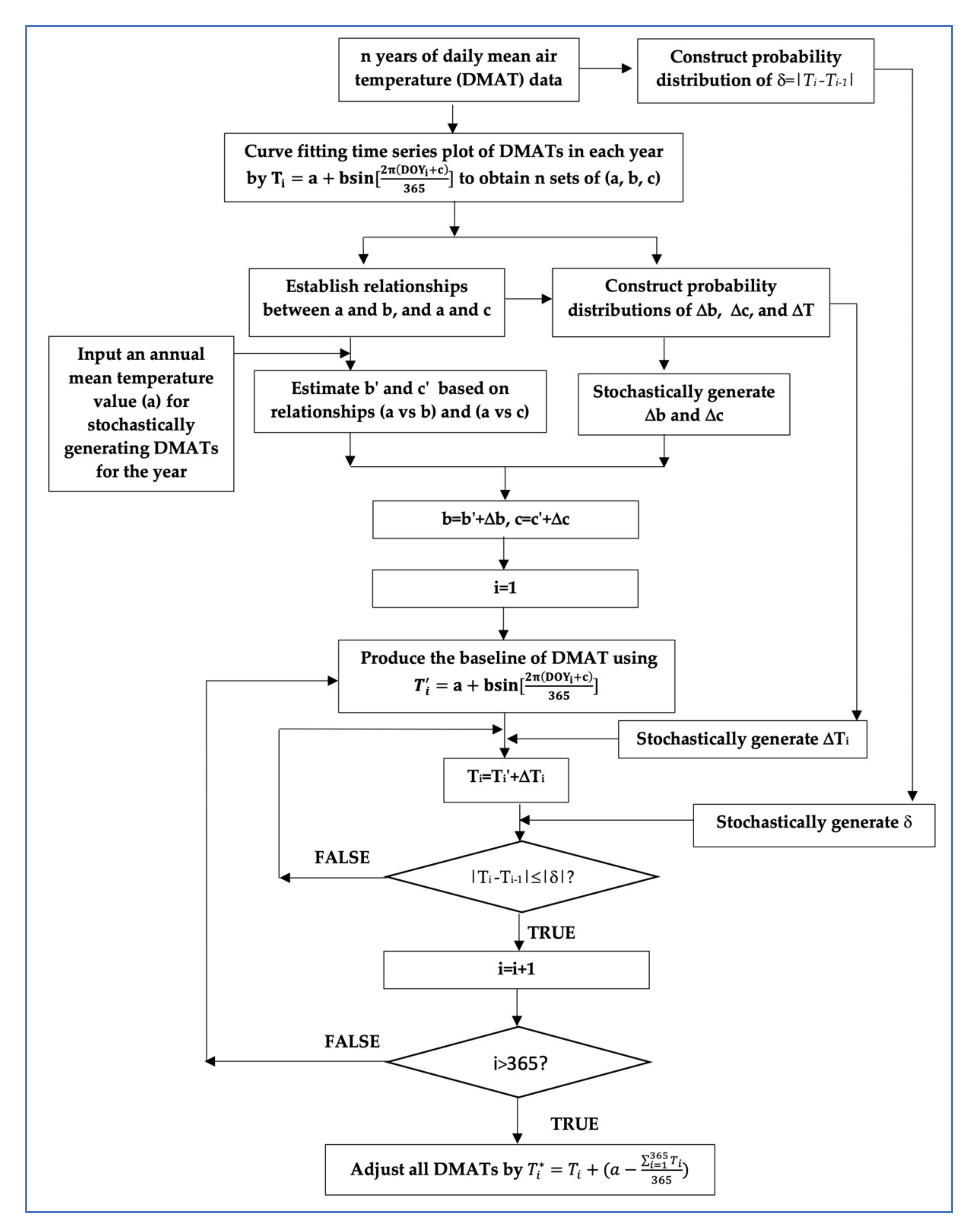
where b′ and c′ are estimated values using the constructed relationships between a and b, and a and c, and and are stochastically generated residual terms based on the probability distributions of . There are four major steps involved in stochastically producing DMAT by the CSWG, as illustrated in Figure 1.
The first step is to apply the sinusoidal wave function of DOY as shown in Equation (1) to fit the time series plot of each year′s DMATs of n years of temperature data (n is the number of years of observed temperature data for constructing the CSWC for stochastically producing DMATs) and obtain n sets of three parameters (i.e., a, b, c). The second step is to establish the relationships between a and b, and a and c using the regression analysis method, and then construct the probability distributions of residual terms , , and . To ensure that the stochastically generated DMATs have a comparable lag-one autocorrelation magnitude as the observed DMATs (i.e., the current day temperature should correlate to the previous day temperature to some degree), the probability distribution of the DMAT difference between two consecutive days (i.e., δ = Ti − Ti−1) is also constructed in this step.
The third step is a loop starting from the first day of the year (i = 1) to the last day of the year (i = 365 or 366) for stochastically producing each day DMAT through adding a randomly generated based on the constructed probability distribution of to the randomly generated baseline DMATs of the year. Prior to moving to the next day, the absolute value of the DMAT difference between the stochastically generated current day and previous day temperatures (i.e., |Ti − Ti−1|S) is computed and compared with a randomly generated |δ| based on the probability distribution of δ: if |Ti − Ti−1|S> |δ|, reject the current stochastically generated Ti and stochastically re-generate a new Ti, and a new δ. If |Ti − Ti−1|S , accept the re-generated Ti as the current day DMATi and move to the next day for producing DMAT, otherwise re-generate a Ti and a δ, till the condition of |Ti − Ti−1|S is satisfied. After all daily temperatures are produced, a final adjustment of all DMATs is necessary to set their average and the given annual mean temperature (i.e., a) equal using the equation
where is the final stochastically generated daily mean air temperature of day i.
4.2. Stochastically Generating Daily Precipitation Based on Annual Precipitation
The function of stochastically generating daily precipitation (DP) based on annual precipitation in the CSWG was developed based on the following assumptions: (1) For each month, the total precipitation can be estimated from annual precipitation if there exists a relationship between the annual precipitation and monthly precipitation. (2) For each month, number of dry days and the maximum daily precipitation can be estimated from the total precipitation in that month. (3) A probability distribution of daily precipitation amount for each wet day can be constructed.
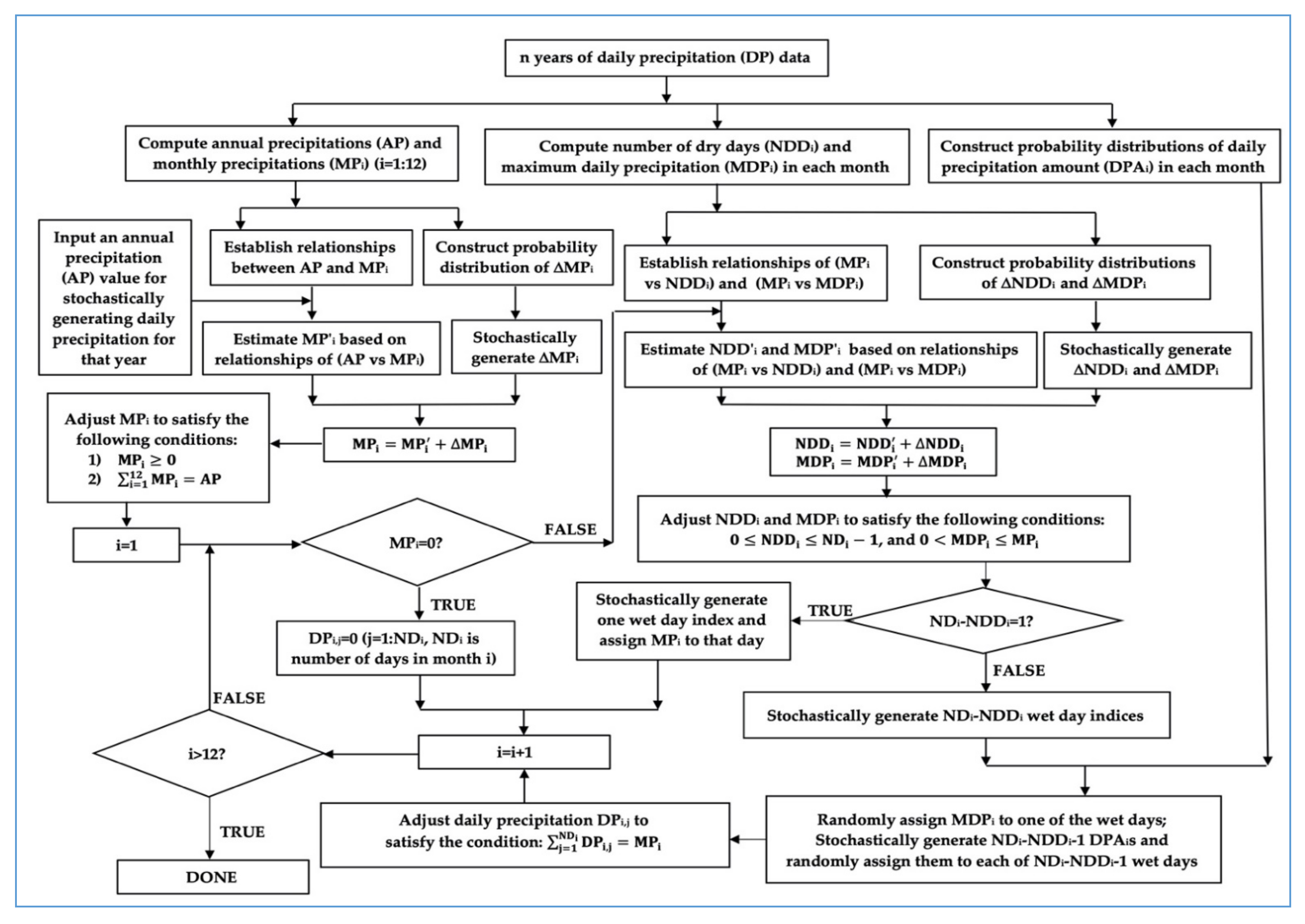
There are four major steps in the CSWG for stochastically generating daily precipitation, as illustrated in Figure 2. The first step is to use n years of observed daily precipitation data to compute annual precipitation (AP) and 12 monthly precipitations (MP) in each year, and number of dry days (NDD) and maximum daily precipitation (MDP) in each month, and construct the probability distribution of daily precipitation amount (DPA) of each month. The second step is to establish relationship between annual precipitation and one of 12 monthly precipitation of that year through the regression analysis and construct the probability distribution of the residual term ΔMP (i.e., difference between the observed and estimated monthly precipitation). In each month, relationships of (MP vs. NDD) and (MP vs. MDP) are also established through the regression analysis and the probability distributions of the residual terms ΔNDD and ΔMDP are subsequently constructed. With a series of the established relationships and probability distributions, the third step is to stochastically generate 12 monthly precipitations from an input annual precipitation. The stochastically generated monthly precipitations are adjusted to satisfy the two conditions: (1) no monthly precipitation is negative; and (2) summation of 12 monthly precipitations is equal to the input annual precipitation.
The fourth step is a loop of stochastically generating daily precipitation in each month starting from January to December. If the stochastically generated monthly precipitation is zero, every day precipitation amount is set to be zero in the month. Otherwise, number of dry days (NDD) and maximum daily precipitation (MDP) are randomly generated based on the relationships of (MP vs. NDD) and (MP vs. MDP) and the probability distributions of ΔNDD and ΔMDP. The randomly generated NDD and MDP are also adjusted to satisfy the following conditions: 0 and 0, ND is the number of days in the month. If the number of wet days (i.e., ND-NDD) is equal to 1, randomly generate an integer number between 1 and ND and use that integer as the wet day index, and assign MP to the precipitation amount of that day. Otherwise, randomly generate ND-NDD integers between 1 and ND and use them as the wet day indices, randomly assign MDP to one of the wet days, and stochastically generate ND-NDD-1 daily precipitation amounts (DPA) based on the probability distribution of DPA, and assign them to ND-NDD-1 wet days. After all wet days are assigned a precipitation amount, the adjustment of daily precipitation (DP) in the month is carried out to ensure that the summation of stochastically generated daily precipitations is equal to the stochastically generated monthly precipitation.
5. Application of the CSWG to Stochastically Generating DMAT and DP
5.1. Stochastically Generating DMAT Using the CSWC
As introduced in Section 3, the daily mean air temperature (DMAT) data collected at Cortez from 1930 to 2016 with less than 10% missing data in each year were used to build the CSWC for stochastically generating DMAT. For the years with less than 10% missing data, the linear interpolation method was applied to fill the data gaps between known data points. Between 1930 and 2016, there are 74 years with less than 10% missing data in each year. After all data gaps were filled, Equation (1) was applied to best fit each of the 74 time series plots of daily air temperatures and obtain three parameters (i.e., a, b, and c) for each year as listed in Table 1.
Based on the extracted three parameters of the sinusoidal wave function of DMAT with respect to DOY as listed in Table 1, the linear regression method was employed to fit the scatter plots of a vs. b and a vs. c, separately, and yielded
The statistics of the linear regressions are listed in Table 2.
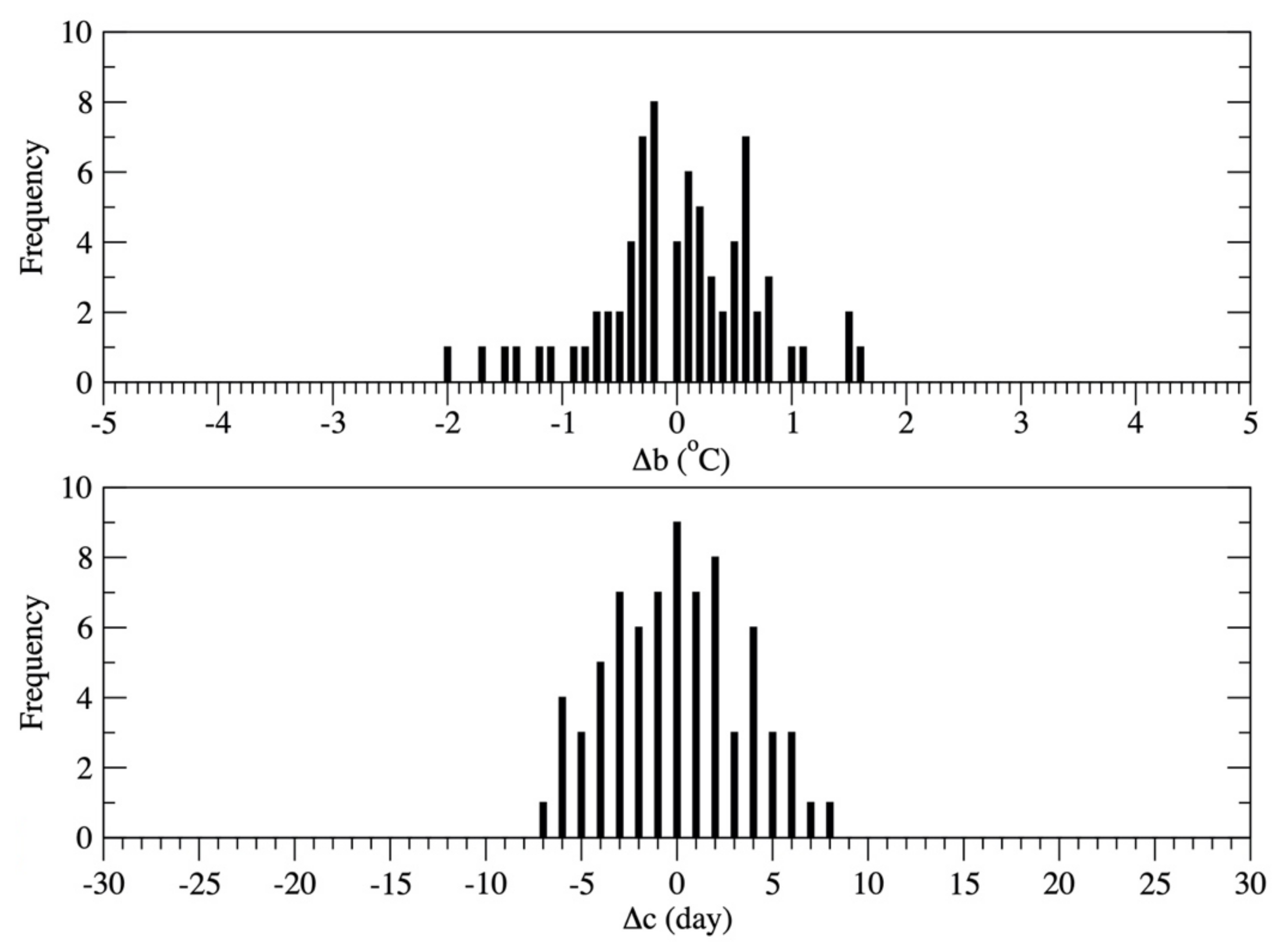
Although the root mean square errors (RMSEs) are small, i.e., 0.69 °C and 3.4 day for the estimated b and c values, respectively, the correlation coefficients are very low (i.e., 0.25 and 0.13), which indicates that the uncertainty in the linear regression equations should be considered as we estimate b and c from a. The uncertainties in the estimated b and c can be represented by the probability distribution of discrepancies between the observed b and c vs. estimated b and c values, i.e., the residual elements. The probability distribution of the residual term Δb is defined as the number of years with Δb within a certain range (i.e., bin) as given below
where Δbi is the possible difference between the observed b and estimated b values within a bin of 0.1 °C. As shown in Table 2, the Δb ranged from −1.96 °C to 1.61 °C. Similarly, the probability distribution of Δc is defined as
where Δci is the possible difference between the observed c and estimated c values within a bin of one day. The difference between the observed c and estimated c ranged from −6.9 day to 7.9 day (see Table 2). The probability distributions of Δb and Δc are shown in Figure 3.
Based on the probability distributions of Δb and Δc, two one-dimensional arrays were produced, each with a length of 74 (because of 74 samples from the DMAT datasets), and the elements of one array are Δb and the elements of the other array are Δc. The number of a particular Δb or Δc appearing in the array depends on the occurrence frequency of that Δb or Δc, e.g., if the frequency is 6 for Δb = 0.1, then 0.1 would appear 6 times in the array. Using these two arrays and the linear regression equations (i.e., Equation (4)), a baseline of DMAT can be generated from an input of annual mean air temperature i.e., (a). For example, if a is 9.5 °C, according to Equation (4), b = 12.7 °C and c = 255.9 day. Next, two integers between 1 and 74 were randomly generated, one for Δb and one for Δc. For example, using the randomly generated numbers 30 and 63 as the array indices to determine the elements in the Δb and Δc arrays, which are −0.20 °C and 4.0 days respectively. Next, a float number was randomly generated in the range of [−0.25, −0.15] for Δb, and a float number was randomly generated in the range of [3.5, 4.5] for Δc. For example, Δb = −0.19 °C, Δc = 4.1 day, and thus b = 12.7 − 0.19 = 12.51 °C and c = 255.9 + 4.1 = 260.0 day. Finally, the randomly generated b and c, along with the input annual mean air temperature (a) were substituted into the sinusoidal wave function as shown in Equation (1) to produce the baseline of DMAT.
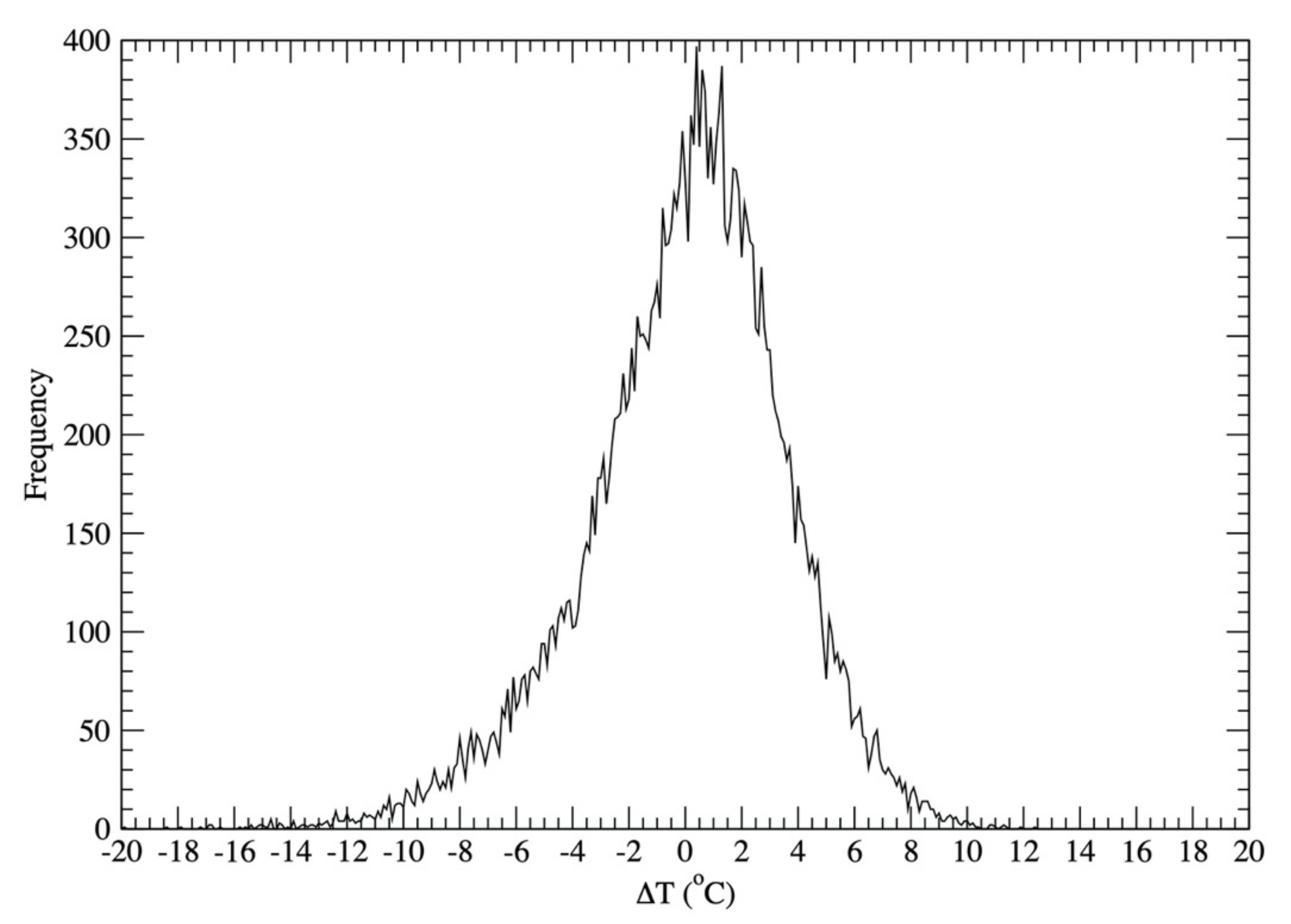
To stochastically generate DMAT, in addition to the baseline of DMAT, a randomly generated temperature perturbation from the baseline for each day is also needed. Using 74 years of DMAT data and the associated baselines, observed DMATs for each year were subtracted from each year baseline temperatures, resulting in 26,997 temperature difference data points (i.e., ΔT). These 26,997 data points were used to construct the probability distribution of ΔT as
where ΔT is in the range of [−19.9 °C, 12.4 °C] with an interval of 0.1 °C. The constructed probability distribution of ΔT is plotted in Figure 4. Based on the computed probability distribution of ΔT, a one-dimensional array with 26,997 elements was generated. The number of a particular ΔTi appearing in the array depends on the occurrence frequency of that ΔTi. Using this ΔT one-dimensional array, temperature perturbation for each day was produced through randomly generating an integer number between 1 and 26,997, and using the randomly generated integer number as the ΔT one-dimensional array index to determine ΔT.
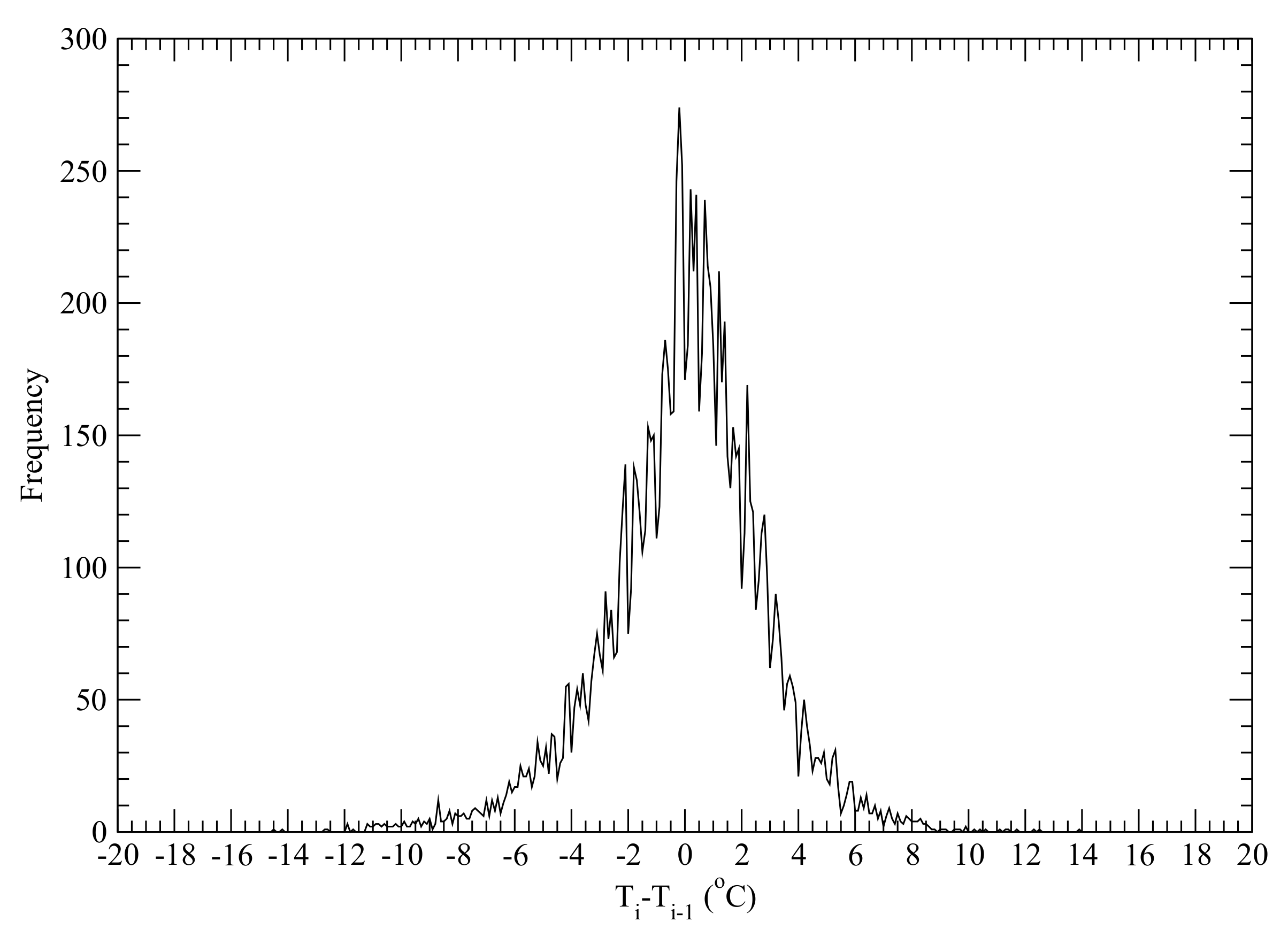
As discussed in Section 4.1, to ensure that the stochastically generated DMATs have a comparable lag-one autocorrelation magnitude as the observed DMATs, the GSOD data were used to compute daily mean air temperature difference δ (= Ti − Ti−1) between two consecutive days (the GHCN temperature data were not used in computing δ because the GHCN daily mean temperatures were estimated from the observed daily maximum and minimum temperatures). The 11,468 computed δs were used to calculate the probability distribution of δ as
where δ is in the range of [−14.5 °C 13.9 °C] with an interval of 0.1 °C. The probability distribution of δ is plotted in Figure 5. Based on the calculated probability distribution of δ, a one-dimensional array with 11,468 elements was created. The number of a particular δi appearing in the array depends on the occurrence frequency of that δi.
5.2. Stochastically Generating DP Using the CSWC
5.2.1. Estimate Monthly Precipitation from Annual Precipitation
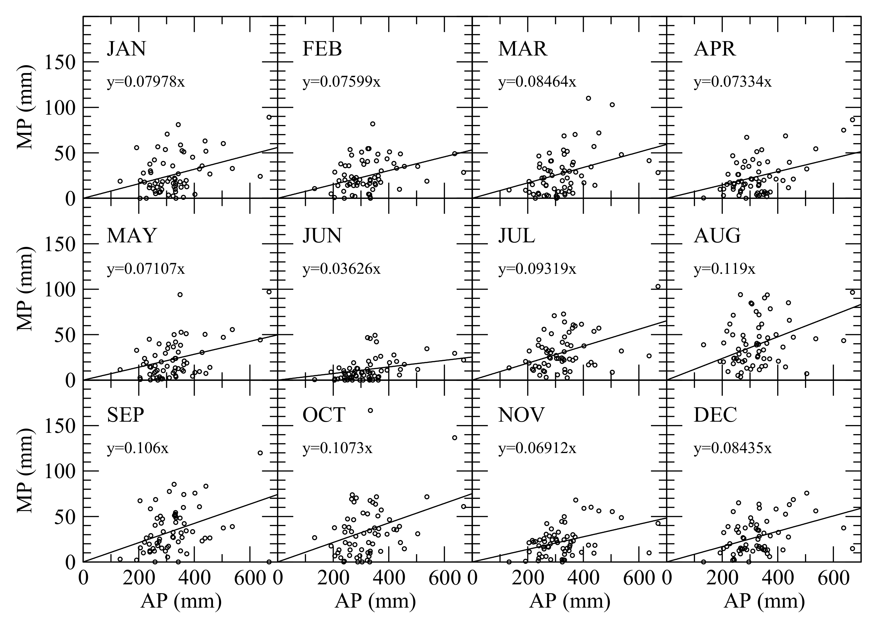
As described in Section 4.2, the first step for stochastically generating daily precipitation (DP) is to estimate monthly precipitations based on annual precipitation, and thus a linear regression method was applied to establish a relationship between each monthly precipitation with the annual precipitation as
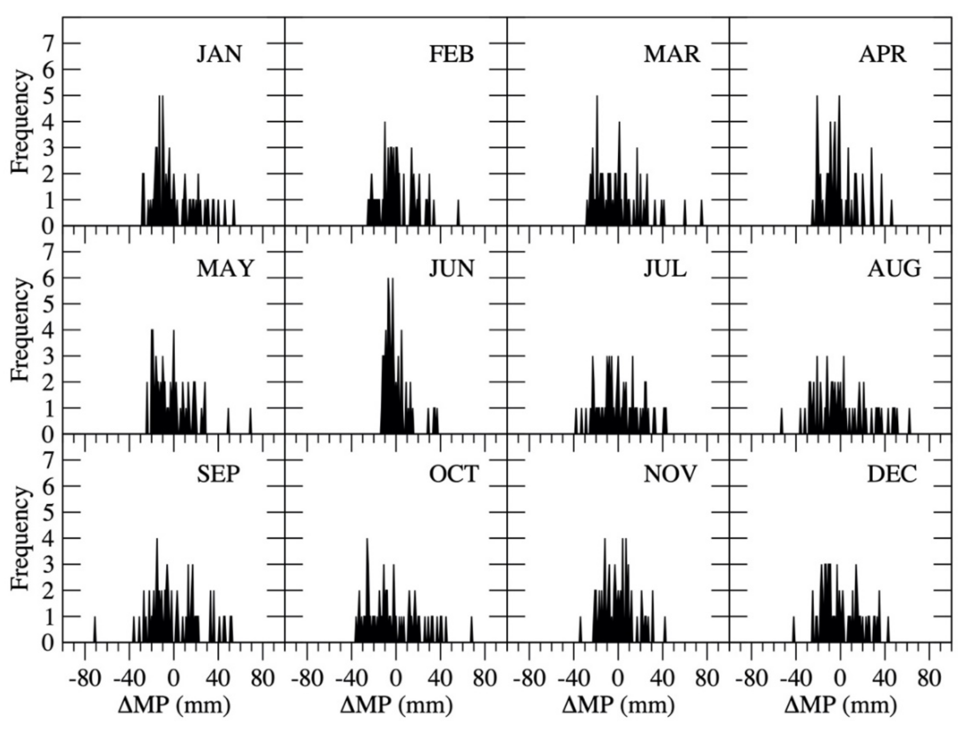
where MPi is the observed total precipitation in month i, AP is the observed annual total precipitation, and fi is the ratio of the total precipitation in month i to the annual precipitation. The precipitation data used for establishing the relationship as shown in Equation (8) were from 1930 to 2016 daily precipitation measurements collected by the GHCN at Cortez, Colorado. Among those 86 years, there are 21 years missing more than 10% precipitation data, and thus only 65 years of GHCN’s precipitation data were used for the regression analysis. The scatter plots and linear regression results of annual precipitation vs. monthly precipitation of 12 months are shown in Figure 7, and the statistics of the linear regressions are listed in Table 3. The low correlation coefficients shown in Table 3 indicate that a simple linear regression cannot capture the monthly precipitation variations with adequate accuracy, thus the difference between the observed and estimated monthly precipitations (ΔMP) should be considered for producing monthly precipitation from annual precipitation through computing the probability distribution of ΔMP as
where the range of MPi (i = 1, …, 12) is listed in Table 3. The probability distribution of each month’s MP is plotted in Figure 8. Using the probability distribution, a one-dimensional MP array was produced for each month with a length of 65 (because of 65 samples). The number of a particular MP value appearing in the one-dimensional array depends on the occurrence frequency of that MP value.
With the regression equations and the one-dimensional ΔMP array for each month, monthly precipitation can be estimated from observed annual precipitation based on the equation
where ΔMPi is generated through randomly selecting an array index between 1 and 65 and using the array index to determine the median ΔMPi value, and then randomly generating a float number between (ΔMPi − 0.5, ΔMPi + 0.5). If the randomly generated MPi value was negative, MPi was set to be zero. After each randomly generated monthly precipitation was estimated, checked, and set to zero when appropriate, it was necessary to determine if the sum of estimated monthly precipitations matched the observed annual precipitation. If they did not match, the difference between them was equally divided by 12 and subtracted (or added) from each monthly precipitation MP as appropriate. The difference between the sum of estimated monthly precipitations vs. observed annual precipitation was recalculated until the difference was less than 0.01 mm.
5.2.2. Estimate Number of Dry Days in Each Month
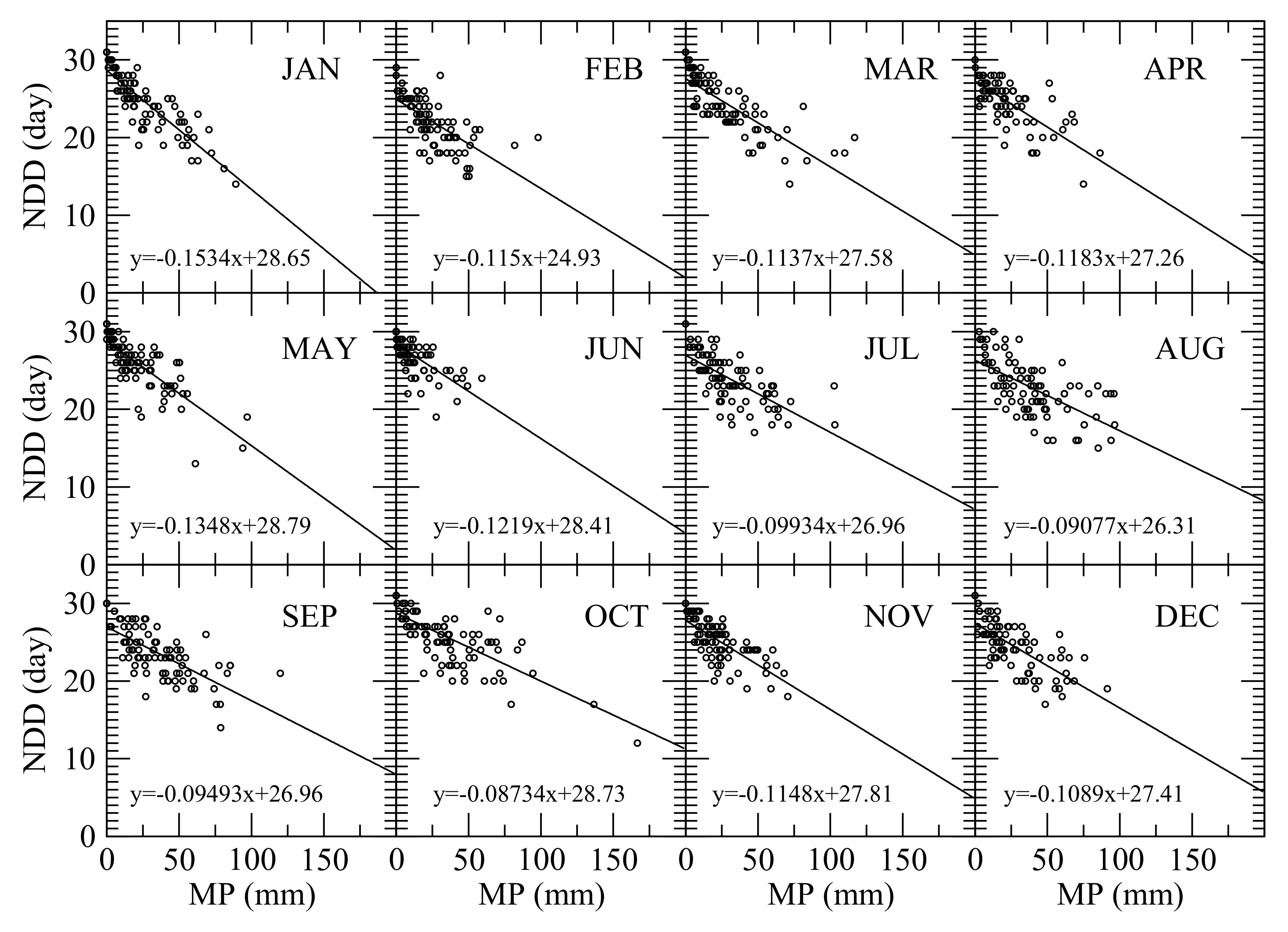
A ‘dry day’ is defined as the one with precipitation less than a trace of rain, which is 0.254 mm in this study. To estimate number of dry days in each month, the GHCN precipitation data were used to count the number of dry days in each month in each year. Scatter plots of monthly precipitation vs. observed number of dry days (NDD) in each month were presented in Figure 9, showing an inverse relationship between monthly precipitation and number of dry days for each month. Therefore, the following linear equation was used to fit each scatter plot
where NDDi is the number of dry days in month i, gi is the slope of the regression line, and NDi is the number of days in month i. By forcing the best-fit line to pass through the point (0, NDi), it can be assured that if the monthly precipitation is zero, the number of dry days is equal to the number of days in that month.
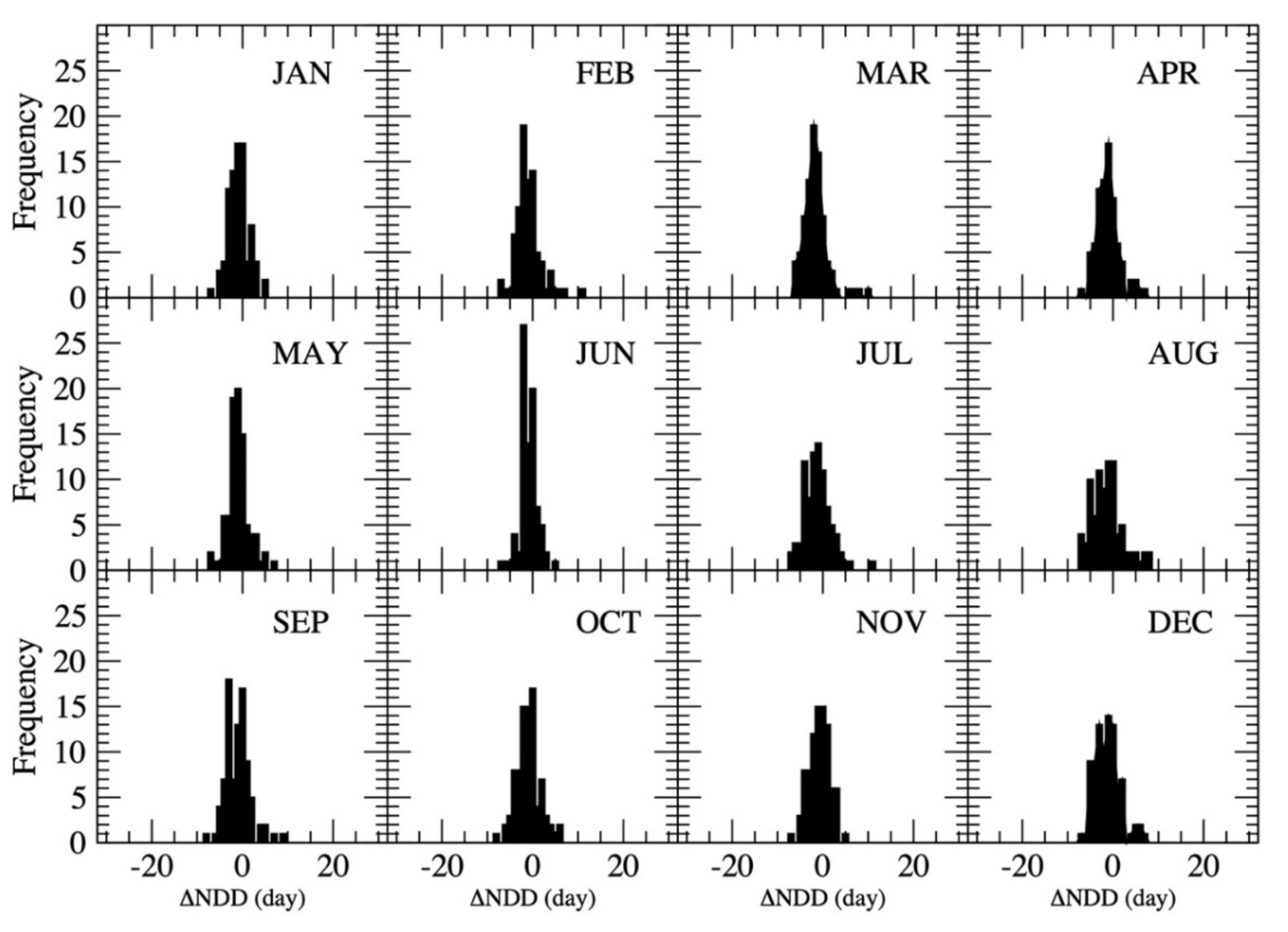
The statistics of the regression analyses of the monthly precipitation vs. the number of dry days are listed in Table 4. To consider the uncertainty in the estimated NDD from MP based on Equation (11), a probability distribution of the difference between the observed and estimated numbers of dry days (ΔNDD) was developed as
where the range of ΔNDD is listed in Table 4. The probability distribution of each month’s ΔNDD is plotted in Figure 10. Using the probability distribution, a one-dimensional array of ΔNDD for each month with a length of 65 was produced. With the regression equations and the one-dimensional ΔNDD array for each month, the number of dry days in each month was estimated from monthly precipitation based on the equation
where ΔNDDi was created through randomly generating an integer between 1 and 65, and using the integer as the array index to determine the median ΔNDDi value, and then randomly generating a number between (ΔNDDi − 0.5, ΔNDDi + 0.5) to represent ΔNDDi in Equation (14). Since the number of dry days in each month should be between 0 and NDi, if NDDi was less than zero, set NDDi = 0, and if NDDi was greater than NDi, set NDDi = NDi.
5.2.3. Estimate Maximum Daily Precipitation in Each Month
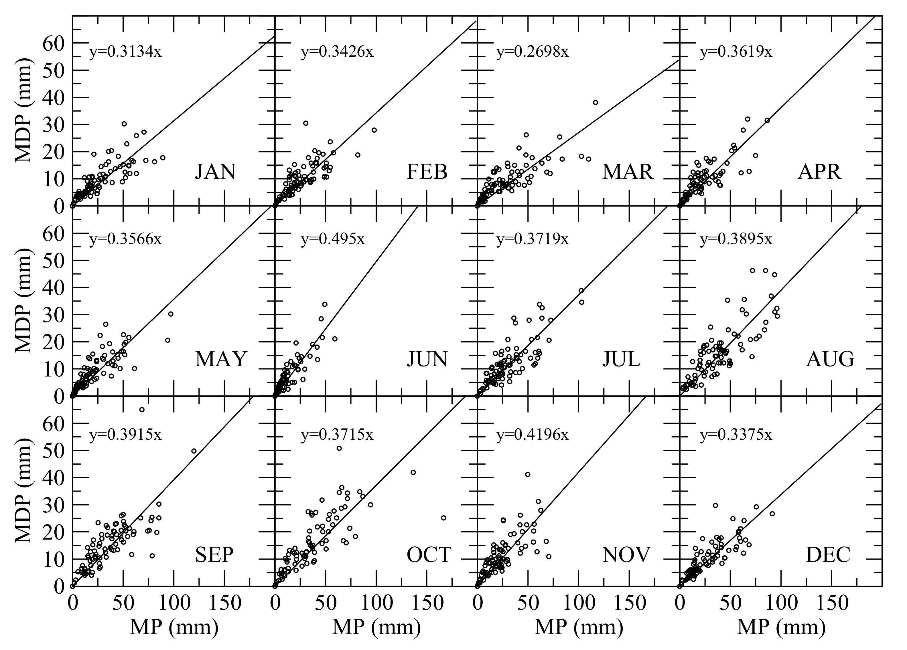
To estimate the maximum daily precipitation, the observed maximum daily precipitation in each month in each year was regressed against observed total monthly precipitation, as shown in Figure 11. The positive linear relationship between monthly precipitation and the maximum daily precipitation of each month suggests a line passing the origin (0, 0) to fit each scatter plot as given in the equation
where MDPi is the maximum daily precipitation and hi is the ratio of the maximum daily precipitation to the monthly precipitation of month i. The statistics of the regression analyses between MP and MDP are listed in Table 5.
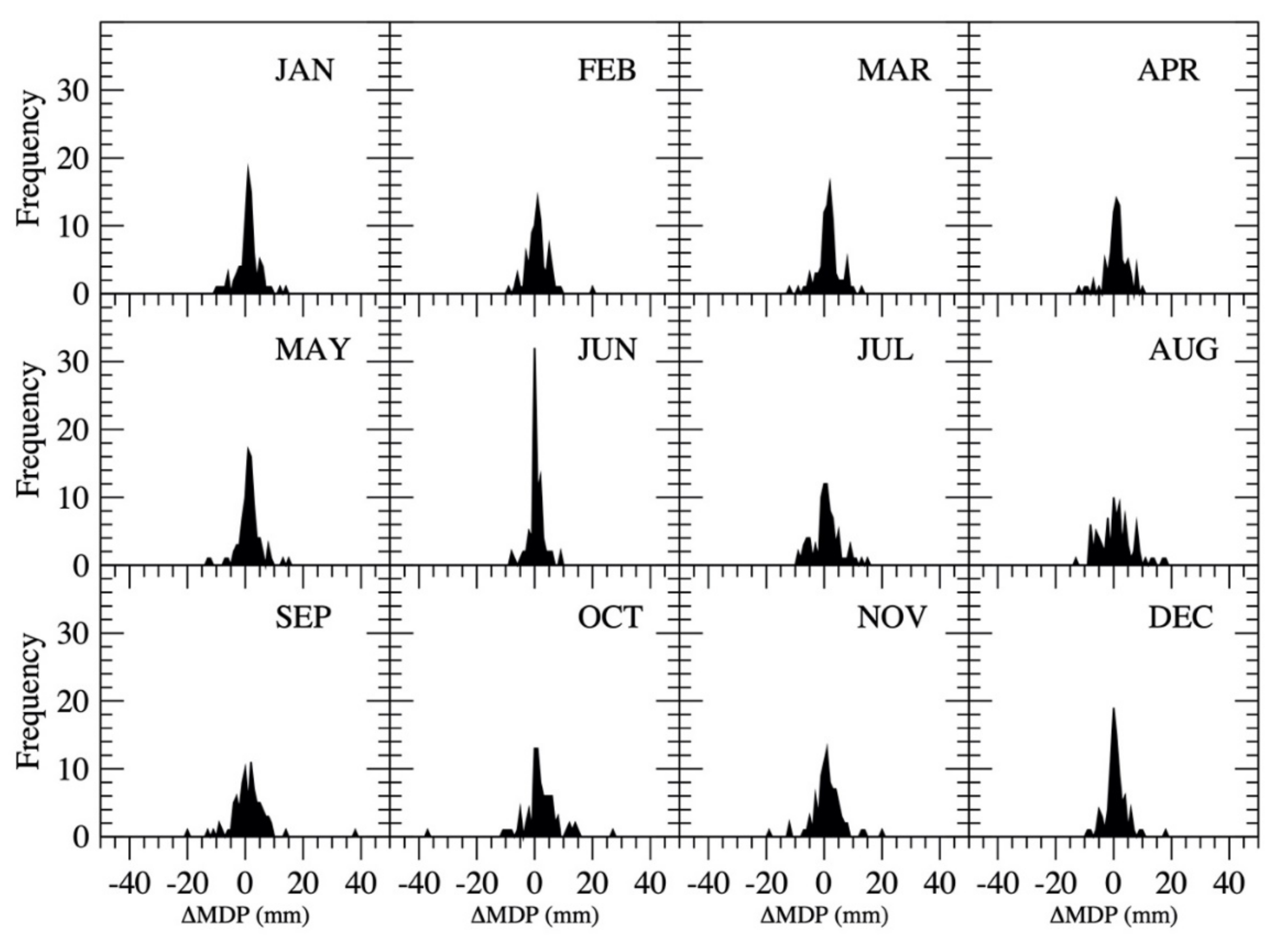
To consider the uncertainty in the estimated maximum daily precipitation from the observed monthly precipitation based on the linear regression equations, a probability distribution of the difference (ΔMDP) between the observed and estimated maximum daily precipitation in each month was determined through computing the occurrence frequency of the difference ΔMDP as
where the range of ΔMDP in each month is listed in Table 5. The probability distribution of each month’s ΔMDP is plotted in Figure 12. Using the probability distribution, a one-dimensional array of ΔMDP for each month with a length of 65 was generated. With the regression equations and the one-dimensional array of ΔMDP for each month, maximum daily precipitation in each month was estimated from total monthly precipitation based on the equation.
where ΔMDPi was determined through randomly generating an integer between 1 and 65, and using the integer as the array index to determine the median ΔMDPi value along with randomly selecting a float number between (ΔMDPi − 0.5, ΔMDPi + 0.5). Since the maximum daily precipitation MDPi in each month should be between 0 and the total monthly precipitation MPi, if MDPi was less than zero, MDPi was set to zero; and if MDPi was greater than MPi, MDPi was set to MPi.
5.2.4. Construct the Probability Distribution of Daily Precipitation Amount in Each Month
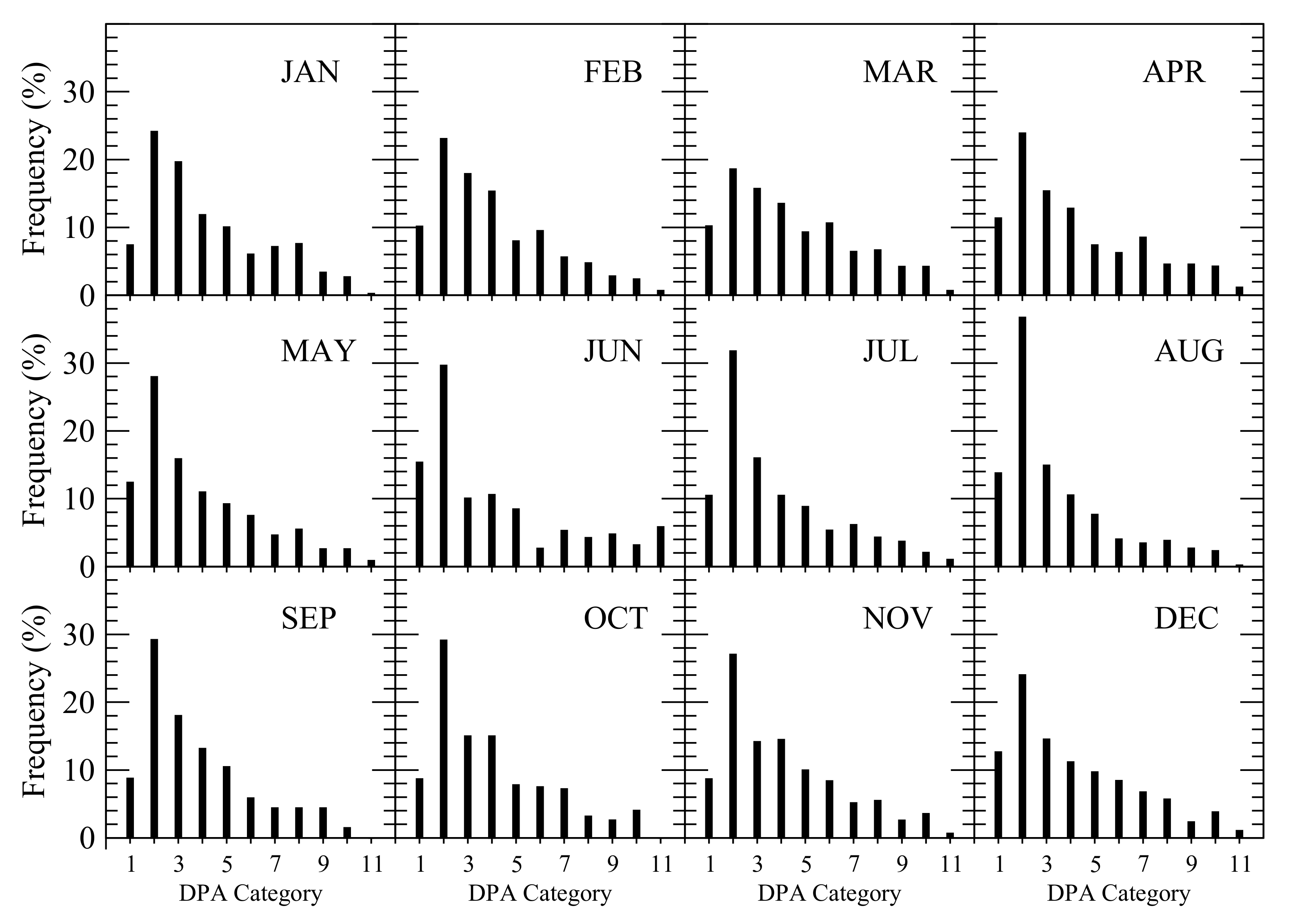
Given the number of dry days and the maximum daily precipitation, stochastically generating daily precipitation in each month is simply a matter of selecting a precipitation amount for each wet day in that month. If the number of wet days was one, the precipitation amount in that wet day was set to be equal to the monthly precipitation of that month (MP). If the number of wet days was more than one, the precipitation amount of one wet day was set to be the maximum daily precipitation of the month (MDP), and the possible precipitation amounts for all other wet days fell in the range of the trace amount of precipitation (i.e., 0.01 inch or 0.254 mm) to the maximum daily precipitation MDP. To stochastically generate daily precipitation amount for each wet day, the number of wet days with the precipitation amount falling in one of 11 categories was determined, as listed in Table 6. These 11 categories include 10 daily precipitation amount (DPA) ranges and one category of trace rain. The probability distribution of the 11 categories of daily precipitation in each month is shown in Figure 13. Using the probability distribution, a one-dimensional array of daily precipitation categories with a length of 1000 was developed for each month, with the number of each daily precipitation category appearing in the array set equal to the occurrence frequency (%) multiplied by 10.
5.2.5. Stochastically Generate Daily Precipitation
Daily precipitation in each month was generated based on the following rules:
- If monthly precipitation MP is zero, every day has zero precipitation in the month.
- If there is only one wet day, the precipitation amount of the wet day is equal to MP.
- If there is more than one wet day, a randomly selected wet day’s precipitation is set to be the maximum daily precipitation MDP. The precipitation amounts of other randomly selected wet days are assigned based on the probability distribution of daily precipitation category, through randomly generating an integer between 1 and 1000, and using the randomly generated integer as the array index to determine the daily precipitation amount category. If it is category 1, the daily precipitation is set to the trace rainfall (0.254 mm); otherwise, based on the daily precipitation amount range of the category defined in Table 6, a randomly generated float number within the daily precipitation amount range of the category is used.
- For each month, after all wet days are assigned a precipitation amount, total precipitation in the month is compared to the estimated MP from annual precipitation. If the difference between them is greater than a threshold (0.01 mm), precipitation amounts of all wet days are adjusted through subtracting or adding the difference divided by the number of wet days. Since each adjusted daily precipitation amount should be between trace precipitation (0.254 mm) and the maximum daily precipitation (MDP), sometimes more than two iterations are needed for adjusting daily precipitation amounts.
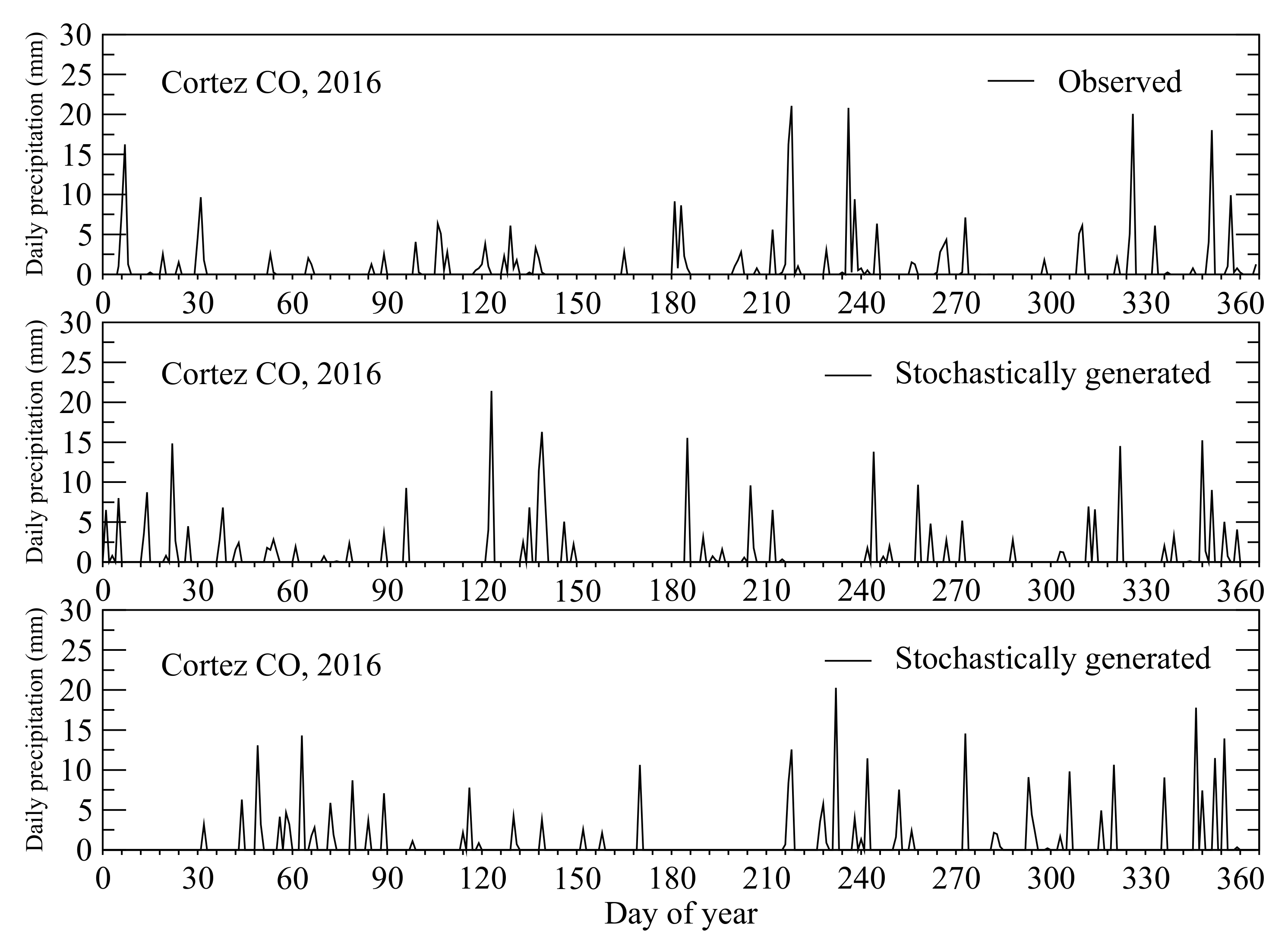
Two sets of stochastically generated daily precipitations as examples for illustrating results, along with the observed daily precipitations in year 2016 at Cortez are shown in Figure 14.
6. Conclusions
This study developed a CSWG for producing daily mean air temperatures and daily precipitations in a year with known or specified annual mean air temperature and annual precipitation. Since there appear to be no other published weather generators that utilize annual mean air temperature or annual precipitation as constraints to daily weather predictions, we believe we are presenting a unique method that researchers can use to explore historic (e.g., archeological questions) or future (e.g., climate change) daily weather conditions based upon specified annual values. Thus, in areas such as the American Southwest where tree-ring chronologies are widely available, a similar weather generator could be developed for specific locations and then used to model daily mean air temperature and daily precipitation for a specific year. These data could then be employed in a variety of paleo-environmental models.
How to validate our CSWG results is a challenging question. Since none of the published SWGs used the annual mean air temperature and precipitation as constraints to daily weather predictions, it is hard to directly compare our results with results produced by other SWGs. On the other hand, it is not proper to directly compare the stochastically generated daily temperatures and precipitations with the observed daily data on the daily basis, and thus some commonly used errors—such as root mean square error or relative error—cannot be utilized in the evaluation of our results. Our CSWG results share the same annual mean temperature and annual precipitation (i.e., the first order moments) as the observations, and the higher order moments may not be the same. Therefore, comparisons of the higher order moments between the observed and stochastically generated daily mean temperature and precipitation data might be necessary. In addition to high order moments, some other statistical characteristics of stochastically generated daily weathers need to be evaluated, which deserve a future systematic study.
After the criteria for evaluating our CSWG results are established, further improvements in the CSWG can be carried out, such as including the correlation between daily temperature and precipitation in the daily temperature generator, and considering the dependencies of the current day′s wet/dry conditions on the previous day′s wet/dry conditions in the daily precipitation generator. Additionally, a future study is necessary to assess the effectiveness and applicability of the CSWG developed in this study in other climatic regions, e.g., tropical, mesothermal, microthermal, and polar.
Author Contributions
F.P., L.N., S.W., and S.F.A. conceived and designed the study; F.P., L.N., S.W., S.F.A., T.A.K., and M.O. analyzed the climate data and developed the constrained stochastic weather generator; F.P. wrote the paper; L.N., S.W., S.F.A., T.A.K., and M.O. revised the paper. All authors have read and agreed to the published version of the manuscript.
Funding
This research was funded by the National Science Foundation (no.1460122).
Informed Consent Statement
Not applicable.
Data Availability Statement
The data presented in this study are available on request from the corresponding author.
Acknowledgments
The authors would like to thank two anonymous reviewers for their constructive comments and suggestions.
Conflicts of Interest
The authors declare no conflict of interest.
Abbreviations
| AP | annual precipitation |
| CSWG | constrainted stochastic weather generator |
| DMAT | daily mean air temperature |
| DOY | day of year |
| DP | daily precipitation |
| DPA | daily precipitation amount |
| GHCN | global historical climate network |
| GSOD | global summary of day |
| MDPi | maximum daily precipitation in month i |
| MPi | monthly precipitation in month i |
| NDi | number of day in month i |
| NDDi | numbere of dry days in month i |
References
- Jones, C.A.; Kiniry, J.R. CERES-Maize; A simulation Model of Maize Growth and Development; Texas A&M University Press: College Station, TX, USA, 1986; 194p. [Google Scholar]
- Amir, J.; Sinclair, T.R. A model of the temperature and solar-radiation effects on spring wheat growth and yield. Field Crop. Res. 1991, 28, 47–58. [Google Scholar] [CrossRef]
- Carberry, P.S.; Muchow, R.C. A simulation model of kenaf for assisting fibre industry planning in Northern Australia. III. Model description and validation. Aust. J. Agric. Res. 1992, 43, 1527–1545. [Google Scholar] [CrossRef]
- Chapman, S.C.; Hammer, G.L.; Meinke, H. A crop simulation model for sunflower. I. Model development. Agron. J. 1993, 85, 725–735. [Google Scholar] [CrossRef]
- Meinke, H.; Hammer, G.L.; Chapman, S.C. A crop simulation model for sunflower. II. Simulation analysis of production risk in a variable sub-tropical environment. Agron. J. 1993, 85, 735–742. [Google Scholar] [CrossRef]
- Dean, J.S.; Van West, C.R. Environment-behavior relationships in southwestern Colorado. In Seeking the Center Place: Archaeology and Ancient Communities in the Mesa Verde region; Varien, M., Wilshusen, R.H., Eds.; University of Utah Press: Salt Lake City, UT, USA, 2002. [Google Scholar]
- Stahle, D.W.; Cook, E.R.; Burnette, D.J.; Torbenson, M.C.A.; Howard, I.M.; Griffin, D.; Díaz, J.V.; Cook, B.I.; Williams, A.P.; Watson, E.; et al. Dynamics, Variability, and Change in Seasonal Precipitation Reconstructions for North America. J. Clim. 2020, 33, 3173–3195. [Google Scholar] [CrossRef]
- Stern, R.D.; Coe, R. A model fitting analysis of daily rainfall data. J. R. Stat. Soc. 1984, 147, 1–34. [Google Scholar] [CrossRef]
- Yang, C.; Chandler, R.E.; Isham, V.S.; Wheater, H.S. Spatial-temporal rainfall simulation using generalized linear models. Water Resour. Res. 2005, 41. [Google Scholar] [CrossRef]
- Furrer, E.M.; Katz, R. Generalized linear modeling approach to stochastic weather generators. Clim. Res. 2007, 34, 129–144. [Google Scholar] [CrossRef] [Green Version]
- Kim, Y.; Katz, R.W.; Rajagopalan, B.; Podestá, G.P.; Furrer, E.M. Reducing overdispersion in stochastic weather generators using a generalized linear modeling approach. Clim. Res. 2012, 53, 13–24. [Google Scholar] [CrossRef] [Green Version]
- Kleiber, W.; Katz, R.W.; Rajagopalan, B. Daily spatiotemporal precipitation simulation using latent and transformed Gaussian processes. Water Resour. Res. 2012, 48, 1–17. [Google Scholar] [CrossRef] [Green Version]
- Verdin, A.; Rajagopalan, B.; Kleiber, W.; Podesta, G.; Bert, F. A conditional stochastic weather generator for seasonal to multi-decadal simulations. J. Hydrol. 2018, 556, 835–846. [Google Scholar] [CrossRef]
- Podesta, G.; Bert, F.; Rajagopalan, B. Decadal climate variability in the Argentine Pampas: Regional impacts of plausible climate scenarios on agricultural systems. Clim. Res. 2009, 40, 199–210. [Google Scholar] [CrossRef] [Green Version]
- Apipattanavis, S.; Bert, F.; Podesta, G.; Rajagopalan, B. Linking weather generators and crop models for assessment of climate forecast outcomes. Agric. For. Meteorol. 2010, 150, 166–174. [Google Scholar] [CrossRef]
- Wilks, D.S.; Wilby, R.L. The weather generation game: A review of stochastic weather model. Prog. Phys. Geogr. 1999, 23, 329–357. [Google Scholar] [CrossRef]
- Gabriel, K.R.; Neumann, J. A Markov chain model for daily rainfall occurrence at Tel Aviv. Q. J. R. Meteorol. Soc. 1962, 88, 90–95. [Google Scholar] [CrossRef]
- Caskey, J.E. A Markov chain model for the probability of precipitation occurrence in intervals of various length. Mon. Weather Rev. 1963, 91, 298–301. [Google Scholar] [CrossRef] [Green Version]
- Stern, H. A system for automated forecasting guidance. Aust. Meteorol. Mag. 1980, 28, 141–154. [Google Scholar]
- Garbutt, D.J.; Stern, R.D.; Dennett, M.D.; Elston, J. A comparison of the rainfall climate of eleven places in West Africa using a two-part model for daily rainfall. Arch. Meteorol. Geophys. Bioclimatol. 1981, 29, 137–155. [Google Scholar] [CrossRef]
- Ahmed, J.; Bavel, C.H.M.; Hiler, E.A. Optimization of crop irrigation strategy under a stochastic weather regime: A simulation study. Water Resour. Res. 1976, 12, 1241–1247. [Google Scholar] [CrossRef]
- Delleur, J.W.; Kavvas, M.L. Stochastic models for monthly rainfall forecasting and synthetic generation. J. Appl. Meteorol. 1978, 17, 1528–1536. [Google Scholar] [CrossRef] [Green Version]
- Nicks, A.D.; Harp, J.F. Stochastic generation of temperature and solar radiation data. J. Hydrol. 1980, 48, 1–17. [Google Scholar] [CrossRef]
- Bruhn, J.A.; Fry, W.E.; Fick, G.W. Simulation of daily weather data using theoretical probability distributions. J. Appl. Meteorol. 1980, 19, 1029–1036. [Google Scholar] [CrossRef] [Green Version]
- Larsen, G.A.; Pense, R.B. Stochastic simulation of daily climatic data. In USDA-SRS, Statistics Research Division Report, No. AGES810831; United States Department of Agriculture: Washington, DC, USA, 1981. [Google Scholar]
- Richardson, C.W.; Wright, D.A. WGEN: A Model for Generating Daily Weather Variables; ARS-8; United States Department of Agriculture, Agriculture Research Service: Washington, DC, USA, 1984; 83p.
- Hayhoe, H.N. Improvements of stochastic weather generators for diverse climates. Clim. Res. 2000, 14, 75–87. [Google Scholar] [CrossRef]
- Jones, P.G.; Thornton, P.K. MarkSim: Software to generate daily rather data for Latin America and Africa. Agron. J. 2000, 92, 445–453. [Google Scholar] [CrossRef] [Green Version]
- Hansen, J.W.; Mavromatis, T. Correcting low-frequency variability bias in stochastic weather generators. Agric. For. Meteorol. 2001, 109, 297–310. [Google Scholar] [CrossRef]
- Racsko, P.; Szeidl, L.; Semenov, M. A serial approach to local stochastic weather models. Ecol. Model. 1991, 57, 27–41. [Google Scholar] [CrossRef]
- Semenov, M.A.; Brooks, R.J.; Barrow, E.M.; Richardson, C.W. Comparison of the WGEN and LARS-WG stochastic weather generators in diverse climates. Clim. Res. 1998, 10, 95–107. [Google Scholar] [CrossRef] [Green Version]
- Semenov, M.A.; Brooks, R.J. Spatial interpolation of the LARS-WG stochastic weather generator in Great Britain. Clim. Res. 1999, 11, 137–148. [Google Scholar] [CrossRef] [Green Version]
- Hanson, C.L.; Cumming, K.A.; Woolhiser, D.A.; Richardson, C.W. Program for Daily Weather Simulation; US Geological Survey Water Resources Investigations: Denver, CO, USA, 1993; 443p. [Google Scholar]
- Hanson, C.L.; Cumming, K.A.; Woolhiser, D.A.; Richardson, C.W. Microcomputer Program for Daily Weather Simulations in the Contiguous United States; ARS-114; US Geological Survey Water Resources Investigations: Denver, CO, USA, 1994; 38p. [Google Scholar]
- Nicks, A.D.; Gander, A.G. Using CLIGEN to Stochastically Generate Climate Data Inputs to WEPP and Other Water Resource Models; US Geological Survey Water Resources Investigations: Denver, CO, USA, 1993; Volume 93–4018, 443p. [Google Scholar]
- Nicks, A.D.; Gander, A.G. CLIGEN: A weather generator for climate inputs to water resources and other models. In Proceedings of the Fifth International Conference on Computers in Agricuture; American Society of Agricultural Engineers: Orlando, FL, USA, 1994; pp. 903–909. [Google Scholar]
- Johnson, G.L.; Hanson, C.L.; Hardegree, S.P.; Ballard, E.B. Stochastic weather simulation: Overview and analysis of two commonly used models. J. Appl. Meteorol. 1996, 35, 1878–1896. [Google Scholar] [CrossRef] [Green Version]
- Smith, R.E.; Schreiber, H.A. Point processes of seasonal thunderstorm rainfall 2. Rainfall depth probabilities. Water Resour. Res. 1974, 10, 418–423. [Google Scholar] [CrossRef]
- Glowacki, D.M. Living and Leaving: A Social History of Regional Depopulation in Thirteenth-Century Mesa Verde; University of Arizona Press: Tucson, AZ, USA, 2015. [Google Scholar]
- Kohler, T.A.; Varien, M.D.; Wright, A.; Kuckelman, K.A. Mesa Verde Migrations New archaeological research and computer simulation suggest why Ancestral Puebloans deserted the northern Southwest United States. Am. Sci. 2008, 96, 146–153. [Google Scholar] [CrossRef]
- Varien, M.D. Depopulation of the Northern San Juan Region. In Leaving Mesa Verde: Peril and Change in the Thirteenth-Century Southwest; Kohler, K.T., Mark, M.D., Wright, A.M., Eds.; University of Arizona Press: Tucson, AZ, USA, 2010; pp. 1–33. [Google Scholar]
- Van West, C.R. Modeling Prehistoric Agricultural Productivity in Southwestern Colorado: A GIS Approach; Washington State University Laboratory of Anthropology: Pullman, WA, USA, 1994. [Google Scholar]
Figure 1.
Flowchart of the CSWG for stochastically generating DMATs.

Figure 2.
Flowchart of the daily precipitation generation in the CSWG.

Figure 3.
Probability distributions of Δb and Δc.

Figure 4.
Probability distribution of ΔT.

Figure 5.
Probability distribution of δ.

Figure 6.
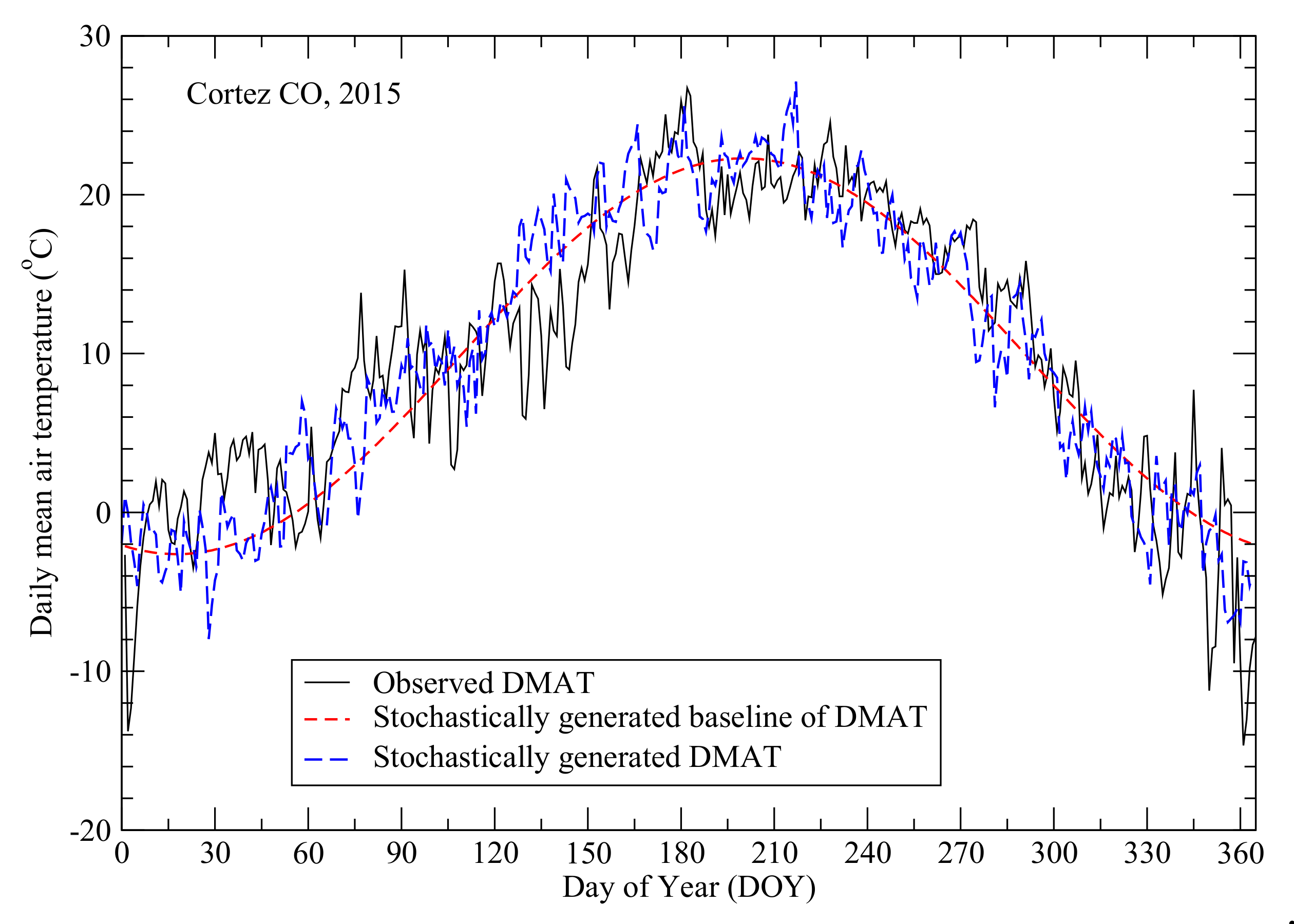
Observed (black) and stochastically generated (blue) daily mean air temperatures of year 2015 at the Cortez station. The red curve is the stochastically generated baseline of daily mean air temperatures of year 2015 at the Cortez station.
Figure 6.
Observed (black) and stochastically generated (blue) daily mean air temperatures of year 2015 at the Cortez station. The red curve is the stochastically generated baseline of daily mean air temperatures of year 2015 at the Cortez station.

Figure 7.
Scatter plots and the best-fit of monthly precipitation vs. annual precipitation.

Figure 8.
Probability distribution of ΔMP.

Figure 9.
Scatter plots and the best-fit line of monthly precipitation (MP) vs. the number of dry days (NDD) in each month.
Figure 9.
Scatter plots and the best-fit line of monthly precipitation (MP) vs. the number of dry days (NDD) in each month.

Figure 10.
Probability distribution of each month’s ΔNDD.

Figure 11.
Scatter plots and the best-fit lines of monthly precipitation (MP) vs. the maximum daily precipitation of each month.
Figure 11.
Scatter plots and the best-fit lines of monthly precipitation (MP) vs. the maximum daily precipitation of each month.

Figure 12.
Probability distribution of each month’s ΔMDP.

Figure 13.
Probability distribution of the 11 categories of daily precipitation amount in each month.
Figure 13.
Probability distribution of the 11 categories of daily precipitation amount in each month.

Figure 14.
Observed and stochastically generated daily precipitations in year 2016.


Table 1.
Three parameters of the sinusoidal wave function for best fitting daily mean air temperatures in 74 years between 1930 and 2016.
Table 1.
Three parameters of the sinusoidal wave function for best fitting daily mean air temperatures in 74 years between 1930 and 2016.
| Year | a (°C) | b (°C) | c (day) | Year | a (°C) | b (°C) | c (day) | Year | a (°C) | b (°C) | c (day) |
|---|---|---|---|---|---|---|---|---|---|---|---|
| 1930 * | 8.68 | 13.26 | 259.7 | 1960 * | 9.83 | 14.15 | 253.9 | 1991 * | 8.26 | 12.66 | 253.3 |
| 1931 * | 8.97 | 13.40 | 255.4 | 1961 * | 9.70 | 13.40 | 259.2 | 1992 | 11.62 | 13.22 | 262.2 |
| 1932 * | 8.58 | 13.46 | 259.6 | 1962 * | 10.25 | 12.25 | 251.4 | 1993 | 12.19 | 12.62 | 262.3 |
| 1934 * | 10.70 | 11.31 | 260.9 | 1963 * | 10.26 | 13.35 | 253.7 | 1995 | 12.36 | 11.35 | 252.0 |
| 1936 * | 9.76 | 12.67 | 258.3 | 1964 * | 9.04 | 13.37 | 251.7 | 1997 | 8.89 | 12.48 | 257.0 |
| 1937 * | 9.01 | 13.92 | 250.7 | 1965 * | 9.49 | 11.31 | 249.0 | 1998 | 9.32 | 12.30 | 252.8 |
| 1938 * | 9.56 | 11.81 | 254.9 | 1966 * | 10.16 | 13.25 | 253.9 | 1999 | 9.32 | 11.21 | 256.1 |
| 1939 * | 9.61 | 13.03 | 253.4 | 1967 * | 9.87 | 12.33 | 255.3 | 2000 | 10.35 | 12.66 | 260.9 |
| 1940 * | 10.07 | 12.72 | 256.9 | 1968 * | 9.10 | 12.53 | 255.9 | 2001 | 9.87 | 12.70 | 258.5 |
| 1941 * | 9.35 | 10.76 | 254.8 | 1969 * | 10.24 | 12.67 | 255.0 | 2002 | 9.56 | 13.45 | 262.5 |
| 1942 * | 9.71 | 12.24 | 249.6 | 1970 * | 9.70 | 12.08 | 253.9 | 2003 | 10.23 | 12.64 | 256.5 |
| 1943 * | 11.36 | 12.33 | 258.3 | 1971 * | 9.41 | 12.81 | 258.2 | 2004 | 9.23 | 12.01 | 261.3 |
| 1944 * | 9.73 | 12.39 | 250.5 | 1972 * | 10.37 | 12.52 | 259.4 | 2005 | 9.63 | 11.44 | 256.7 |
| 1945 * | 9.55 | 12.21 | 253.1 | 1975 | 11.34 | 13.90 | 253.1 | 2006 | 9.63 | 12.46 | 263.5 |
| 1947 * | 9.97 | 12.70 | 256.7 | 1976 | 12.00 | 11.75 | 254.6 | 2007 | 9.81 | 13.20 | 258.1 |
| 1948 * | 9.66 | 12.83 | 253.7 | 1978 | 11.15 | 12.94 | 258.8 | 2008 | 8.83 | 13.16 | 254.3 |
| 1949 * | 9.56 | 13.20 | 253.4 | 1980 | 11.56 | 11.91 | 255.4 | 2009 | 9.22 | 12.60 | 261.7 |
| 1952 * | 9.86 | 13.32 | 253.3 | 1981 | 12.05 | 12.45 | 257.0 | 2010 | 9.13 | 12.79 | 255.3 |
| 1953 * | 10.25 | 12.37 | 252.5 | 1983 | 10.49 | 12.20 | 251.7 | 2011 | 9.27 | 13.32 | 258.0 |
| 1954 * | 11.27 | 11.94 | 256.6 | 1985 | 11.03 | 12.83 | 257.6 | 2012 | 10.42 | 13.11 | 259.6 |
| 1955 * | 9.40 | 12.92 | 249.8 | 1986 | 12.22 | 11.47 | 263.2 | 2013 | 9.10 | 14.26 | 260.8 |
| 1956 * | 9.92 | 12.43 | 256.6 | 1987 | 10.89 | 12.22 | 261.2 | 2014 | 10.10 | 12.06 | 256.6 |
| 1957 * | 9.83 | 10.91 | 255.1 | 1988 * | 8.94 | 13.33 | 251.7 | 2015 | 10.01 | 11.74 | 257.7 |
| 1958 * | 10.68 | 12.25 | 252.4 | 1989 * | 9.22 | 12.96 | 259.3 | 2016 | 9.83 | 12.46 | 256.2 |
| 1959 * | 10.73 | 12.53 | 256.8 | 1990 * | 9.18 | 13.01 | 257.1 |
* Daily mean air temperatures were estimated from observed daily maximum and minimum temperatures collected by the GHCN.
Table 2.
Statistics of the linear regression of a vs. b, and a vs. c.
| a vs. b | a vs. c | |
|---|---|---|
| Root Mean Square Error (RMSE) | 0.69 °C | 3.4 day |
| Correlation Coefficient (r) | 0.25 | 0.13 |
| Maximum (OBS.-EST.) | 1.16 °C | 7.5 day |
| Minimum (OBS.-EST.) | −1.96 °C | −6.9 day |
Table 3.
Statistics of the linear regression of annual precipitation vs. monthly precipitation.
| Month | f | RMSE (mm) | r | Range of ΔMP |
|---|---|---|---|---|
| January | 0.07978 | 19.29 | 0.38 | [−28.0 mm, 54.0 mm] |
| February | 0.07599 | 16.45 | 0.26 | [−25.0 mm, 56.0 mm] |
| March | 0.08464 | 21.13 | 0.43 | [−28.0 mm, 75.0 mm] |
| April | 0.07334 | 16.71 | 0.50 | [−25.0 mm, 46.0 mm] |
| May | 0.07107 | 18.18 | 0.47 | [−24.0 mm, 69.0 mm] |
| June | 0.03626 | 11.09 | 0.41 | [−13.0 mm, 37.0 mm] |
| July | 0.09319 | 18.78 | 0.35 | [−38.0 mm, 43.0 mm] |
| August | 0.119 | 24.76 | 0.15 | [−53.0 mm, 62.0 mm] |
| September | 0.106 | 23.23 | 0.31 | [−71.0 mm, 52.0 mm] |
| October | 0.1073 | 28.22 | 0.38 | [−36.0 mm,131.0 mm] |
| November | 0.06912 | 15.02 | 0.39 | [−34.0 mm, 42.0 mm] |
| December | 0.08435 | 17.87 | 0.34 | [−42.0 mm, 43.0 mm] |
Table 4.
Statistics of the linear regression of MP vs. NDD.
| Month | g | RMSE (day) | r | Range of ΔNDD |
|---|---|---|---|---|
| January | −0.2087 | 2.4 | 0.77 | [−7 day, 5 day] |
| February | −0.1947 | 3.0 | 0.34 | [−7 day, 11 day] |
| March | −0.1811 | 3.2 | 0.48 | [−6 day, 10 day] |
| April | −0.187 | 13.3 | 0.37 | [−7 day, 7 day] |
| May | −0.1911 | 2.6 | 0.65 | [−7 day, 7 day] |
| June | −0.1812 | 2.1 | 0.47 | [−7 day, 5 day] |
| July | −0.189 | 3.2 | 0.29 | [−7 day, 11 day] |
| August | −0.1776 | 3.7 | 0.31 | [−7 day, 8 day] |
| September | −0.1542 | 2.9 | 0.46 | [−8 day, 9 day] |
| October | −0.1293 | 2.8 | 0.62 | [−8 day, 6 day] |
| November | −0.1763 | 2.3 | 0.53 | [−7 day, 5 day] |
| December | −0.1951 | 3.1 | 0.13 | [−7 day, 7 day] |
Table 5.
Statistics of the linear regression of MP vs. MDP.
| Month | h | RMSE (mm) | r | Range of ΔMDP |
|---|---|---|---|---|
| January | 0.3134 | 4.12 | 0.76 | [−10 mm, 14 mm] |
| February | 0.3426 | 4.13 | 0.73 | [−9 mm, 20 mm] |
| March | 0.2698 | 4.30 | 0.75 | [−12 mm, 13 mm] |
| April | 0.3619 | 3.98 | 0.80 | [−12 mm, 10 mm] |
| May | 0.3566 | 4.19 | 0.77 | [−13 mm, 15 mm] |
| June | 0.495 | 2.91 | 0.90 | [−8 mm, 9 mm] |
| July | 0.3719 | 4.79 | 0.81 | [−9 mm, 15 mm] |
| August | 0.3895 | 5.99 | 0.80 | [−13 mm, 18 mm] |
| September | 0.3915 | 6.56 | 0.75 | [−20 mm, 18 mm] |
| October | 0.3715 | 7.33 | 0.74 | [−37 mm, 27 mm] |
| November | 0.4196 | 5.20 | 0.71 | [−19 mm, 20 mm] |
| December | 0.3375 | 3.76 | 0.83 | [−9 mm, 18 mm] |
Table 6.
Eleven categories of daily precipitation amount (DPA).
| Category | DPA Range | Category | DPA Range |
|---|---|---|---|
| 1 | DPA = 0.254 mm (trace) | 7 | 0.55 MDP ≤ DPA < 0.65 MDP |
| 2 | 0.254 mm < DPA < 0.15 MDP | 8 | 0.65 MDP ≤ DPA < 0.75 MDP |
| 3 | 0.15 MDP ≤ DPA < 0.25 MDP | 9 | 0.75 MDP ≤ DPA < 0.85 MDP |
| 4 | 0.25 MDP ≤ DPA < 0.35 MDP | 10 | 0.85 MDP ≤ DPA < 0.95 MDP |
| 5 | 0.35 MDP ≤ DPA < 0.45 MDP | 11 | 0.95 MDP ≤ DPA ≤ MDP |
| 6 | 0.45 MDP ≤ DPA < 0.55 MDP |
Publisher’s Note: MDPI stays neutral with regard to jurisdictional claims in published maps and institutional affiliations. |
© 2021 by the authors. Licensee MDPI, Basel, Switzerland. This article is an open access article distributed under the terms and conditions of the Creative Commons Attribution (CC BY) license (http://creativecommons.org/licenses/by/4.0/).
Share and Cite
MDPI and ACS Style
Pan, F.; Nagaoka, L.; Wolverton, S.; Atkinson, S.F.; Kohler, T.A.; O’Neill, M. A Constrained Stochastic Weather Generator for Daily Mean Air Temperature and Precipitation. Atmosphere 2021, 12, 135. https://doi.org/10.3390/atmos12020135
AMA Style
Pan F, Nagaoka L, Wolverton S, Atkinson SF, Kohler TA, O’Neill M. A Constrained Stochastic Weather Generator for Daily Mean Air Temperature and Precipitation. Atmosphere. 2021; 12(2):135. https://doi.org/10.3390/atmos12020135
Chicago/Turabian StylePan, Feifei, Lisa Nagaoka, Steve Wolverton, Samuel F. Atkinson, Timothy A. Kohler, and Marty O’Neill. 2021. "A Constrained Stochastic Weather Generator for Daily Mean Air Temperature and Precipitation" Atmosphere 12, no. 2: 135. https://doi.org/10.3390/atmos12020135
Note that from the first issue of 2016, this journal uses article numbers instead of page numbers. See further details here.