Simulation of Flexible Fibre Particle Interaction with a Single Cylinder


Department of Engineering Sciences and Mathematics, Division of Fluid and Experimental Mechanics, Luleå University of Technology, SE-971 87 Luleå, Sweden
*
Author to whom correspondence should be addressed.
Processes 2021, 9(2), 191; https://doi.org/10.3390/pr9020191
Submission received: 20 December 2020
/
Revised: 18 January 2021
/
Accepted: 18 January 2021
/
Published: 20 January 2021
(This article belongs to the Collection Modeling, Simulation and Computation on Dynamics of Complex Fluids)
Abstract
:In the present study, the flow of a fibre suspension in a channel containing a cylinder was numerically studied for a very low Reynolds number. Further, the model was validated against previous studies by observing the flexible fibres in the shear flow. The model was employed to simulate the rigid, semi-flexible, and fully flexible fibre particle in the flow past a single cylinder. Two different fibre lengths with various flexibilities were applied in the simulations, while the initial orientation angle to the flow direction was changed between 45° ≤ θ ≤ 75°. It was shown that the influence of the fibre orientation was more significant for the larger orientation angle. The results highlighted the influence of several factors affecting the fibre particle in the flow past the cylinder.
1. Introduction
Fibre suspensions occurs in a wide range of natural and industrial applications. The behaviour of fibre suspensions is a major concern in many industrial applications, such as lubrication, extrusion, and moulding. The orientation and distribution of the fibres are the two most important factors which can determine the rheological behaviour of the fibre suspension. In order to design and control the processes and applications dealing with fibrous suspensions, understanding the description of the fibre orientation pattern is important. Over the past years, many approaches have been presented so far to simulate flexible fibres. The first work on the mechanics of fibres was presented by Yamato and Matsuoka [1,2,3], where the fibres were modelled as a series of connected beads. Further, several models were developed, such as that introduced by Schmid et al. [4], in which the role of shear rate, fibre morphology, fibre flexibility, and frictional-interparticle forces in the flocculation of fibres suspended in a fluid medium were investigated. In Schmid’s model, fibres were modelled as chains of massless fibre segments that interacted with other fibres through contact forces. In this model, the effects of particle inertia, non-creeping fibre-fluid interactions, hydrodynamic interactions between fibres, self-interactions, and the two-way coupling between the fibre and fluid phases were overlooked. In addition, the model suffered from numerical instabilities which seriously restricted the range of simulation parameters. The basic model proposed by Schmid et al. [4] was implemented later in various research, see, e.g., references [5,6,7,8,9,10,11,12,13]. In addition, some other multiphase flow models have been used to study the fibre suspensions; for example in a work by MacMeccan et al. [14], where the original Lattice Boltzmann method was employed. Similar work was performed by Qi [15], in which, due to a high computational cost, only fibres with small aspect ratios were selected. The immersed boundary method [16] has also been used in several studies; see, e.g., references [17,18]. Forgacs and Mason [19] introduced five different regimes of fibre motion that ranged from short and rigid to very long and flexible. According to Arlov et al. [20], the dynamics of flexible fibres were classified into three classes: flexible spin, flexible spin-rotation, and other configurations such as snake turn and springy rotations where the fibres were extremely flexible.
Rigid fibre suspension in Newtonian fluids do not show shear thinning properties, but the flexible fibre suspensions can show this behaviour in a Newtonian fluid [21]. In other words, the rheological properties of the fibrous fluids can be controlled by fibre orientation, distribution, and dispersion. Several models have been developed so far. Shear thinning and shear thickening can be controlled by the aspect ratio of the fibres: a higher aspect ratio shows shear thinning while a lower one controls the shear thickening properties. In addition, it was shown that the yield stress scales with the volume fraction of the fibres in the suspension. Switzer and Klingenberg [22] found that the viscosity can be strongly influenced by fibre equilibrium shape, inter-fibre friction, and fibre stiffness. Chaouche and Koch [17] also examined the effect of shear stress and fibre concentration on the shear thinning behaviour of rigid fibre suspensions. They have shown that fibre bending and a non-Newtonian suspending liquid can play a major role in the shear-thinning behaviour of suspension at high shear rate values.
An understanding of the rheology and dynamics of the deformation of fibrous suspension as a multiphase fluid is important in order to be able to fully disclose the flow behaviour from very low to very high shear rates. To the knowledge of the authors, only a few studies have been done on the study of the fibre orientation through objects [18,23,24]. In the present study, we present the results of the motion of rigid, semi-flexible, and fully flexible fibres with different initial orientation angle.
The first aim of this study is to investigate the fibre dynamics against several orbit classes—i.e., rigid, springy, flexible, and complex rotation of the fibres [19,20,25], enabling the model to have all degrees of freedom (translation, rotation, bending, and twisting, respectively). The second aim is to understand the behaviour of flexible fibres around a cylinder object in very low Reynolds number flows (Re ≤ 1).
In this study, a flexible fibre model has been implemented in an open source computational fluid dynamics code, OpenFOAM. The three-dimensional Navier–Stokes equations, which describe the fluid motion, are employed, and the fibrous phase of the fluid is modelled as chains of fibre segments that can interact with the fluid through viscous and drag forces. This model can be used for further research studies on fibre suspension modelling.
2. Computational Setup and Governing Equations
To simulate the behaviour of single fibre elements around the cylindrical object, first, the flow over a single cylinder in two-dimensional (2D) space was considered and validated. After that, the fibre suspension model was implemented, validated, and applied to the single-phase flow domain.
2.1. Single Phase Flow
The state of the flow in which the single fibre is suspended is steady, laminar, and without secondary motions. This is indeed the case when considering the very low Reynolds number for the flow in the domain. Non-dimension analysing of the governing equations that use the diameter of the cylinder, D, as characteristic length scale and the inlet velocity, U, as characteristic velocity can be shown, as below:
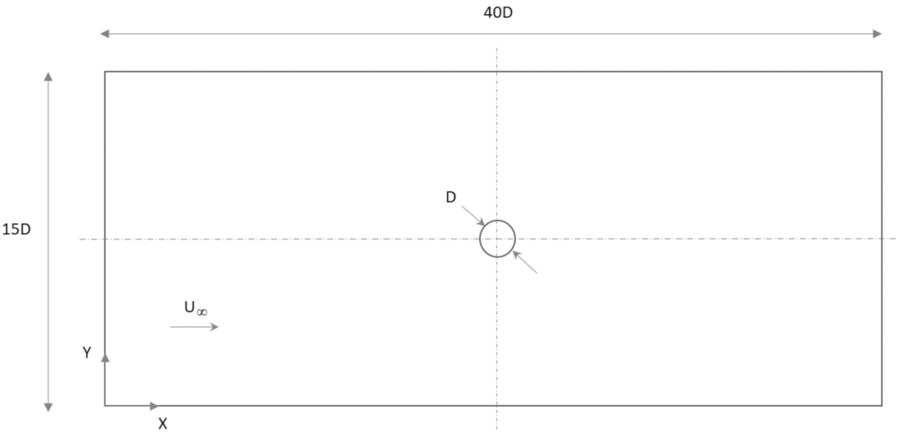
A single cylinder with diameter, D, is considered in a rectangular domain and a cartesian coordinate. Figure 1 shows the domain and the cylinder position. Simulations are carried out for two Reynold’s numbers (Re = 20 and Re = 40). The dimension of the 2D computational domain in all simulations are 15D × 40D. A uniform velocity profile at the inlet, a Dirichlet condition at the outlet, slip boundary conditions at the lateral boundaries, and a no-slip boundary condition on the cylinders surface are applied. A grid sensitivity study of computational domain (Figure 2a) used in this study is obtained. Various simulations of the Newtonian flow past the single cylinder are performed, and the drag coefficient is selected as a criterion to find the grid independent computational domain. It is found that there are only minor differences in the drag coefficients for the three finest resolutions, and the grid resolution of D/20 is employed for all computational calculations, Figure 2b.
Model Validation
For validating the computational solver, the drag coefficient results of the single cylinder in a Newtonian media are compared with the results of the former researchers. Table 1 shows the results for Reynolds numbers Re = 20 and Re = 40. The results of this study agree well with the previous results.
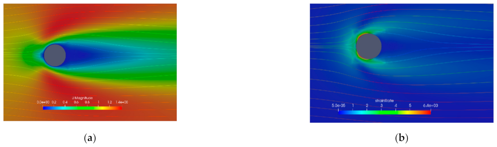
Figure 3 shows the contour plot of the velocity and the shear strain rate around the single cylinder. As the flow passes the cylinder, the minimum velocity occurs at the front stagnation point where the flow has the first contact with the body. The maximum pressure is found in this area. The flow continues around the cylinder, and the velocity increases up to the point in which the flow velocity would reach the maximum value (near 90°). By introducing a fibre particle into this field, the fibre would be affected by several forces, which are discussed in the next section. The forces and momentums move, rotate, twist, and bend the fibre particle and force it to adopt the direction of the flow streamlines.
2.2. Fibre Suspension Model
Figure 4 represents a system of spheroid segments. Following the particle-level method based on Ross and Klingenberg [32], a chain of rigid cylindrical segments has been considered for modelling. The flexible fibres and each segment of the fibre is tracked individually through a Lagrangian Particle Tracking method. For each segment, the translational and rotational equations are solved for each fibre segment by applying Newton’s second law. The model has been implemented in the OpenFOAM open source software [33]. Here, we briefly describe the model.
In Figure 4, the location of each segment is recognized by . The spheroid has a major axis, 2a, and minor axis, 2b. The segments are connected through a ball and socket joint, as illustrated in the figure. The connectivity of the fibres satisfies Equation (3).
Using the connectivity matrix, , Equation (3) can be written in matrix form in Equation (4):
In Equation (4), and is an N × N matrix in which . is a N × 1 matrix of ones. is an N × N connectivity matrix which is defined as:
There is a need to define another connectivity matrix, , defined as:
where
and is an N × N identity matrix. These two connectivity matrices are used to describe the connectivity of the spheroids and joints together. Using Equations (4) and (5), the position of each spheroid reads:
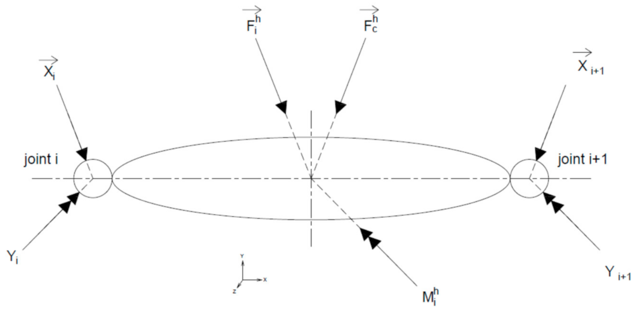
The equations of motion are solved by applying Newton’s second law and the conservation of momentum. Figure 5 shows the free-body diagram for a single fibre spheroid, i. Fi is the resultant force applied to the centre of the mass. This force consists of hydrodynamic forces, , fibre-fibre contact forces, and the body forces. It is worthwhile to note that, in the current model, the two later forces are neglected. In addition, we neglect the fibre inertia in this model. Regarding the contact type, one-way coupling is considered. In other words, the fibres have no influence on their carrier fluid in this model.
To compute the hydrodynamic force, and the hydrodynamic torque, , the theory provided by Kim and Karrila [34] is employed, giving:
In Equations (7) and (8), , , , and are the velocity, vorticity, absolute angular velocity, and strain rate, respectively. , , and are resistance tensors expressed by Equations (9)–(11).
In the equations above, is the identity tensor and is the permutation tensor. , , , , and are a function of the eccentricity (), and they are defined by Equations (12)–(16).
From Figure 4 and Figure 5, one can define the internal torques at the joints between two joints, i and i + 1, i.e., by:
In Equation (17), is the angle between the two spheroids in Figure 4 and is the previous angle at equilibrium status, which is for the straight fibre. is the bending constant which represents the rigidity of the fibre model under the applied bending momentum, such that:
where E is the modulus of elasticity and I is the moment of inertia. As in Equation (17), one can get a similar equation to calculate the twisting torque, . The rigidity against twist torque, is defined by:
where G is the shear modulus and J is the polar moment of inertia.
The final form of the equations of motion is described by:
It should be noted that, in this study, we considered the single fibres as neutral fibres; hence, the body forces are overlooked (see Figure 5), i.e., . In Equation (20), is the external contact force.
From Equations (20) and (21) one can calculate the translational and rotational velocity of a spheroid, i [24], with Equations (22)–(29).
where
In Equations (22)–(29), and the aspect ratio is . For the fibre segments in contact with a surface, I is defined as an identity matrix used to prevent the fibre segment passing the wall. Matrix contains the fibre centre of mass, and matrix represents the position of the centre of the fibre segments relative to the fibre centre of mass. It should be mentioned that all of the equations above have been made dimensionless, employing and for length, time, and force, respectively.
Regarding the flexibility of a fibre particle, a dimensionless shear rate, , is defined as:
To define the fibre-wall contact, the method developed by Vakil and Green [24] is implemented in the code.
Fibre model validation
To validate the fibre model, several simulations are performed, considering various fibre aspect ratios. The results of the rigid fibres are compared with two benchmarks: the experimental results by Forgacs and Mason [19] and the theory of orbit by Jeffery [35], which states that the dimensionless period of rotation is dependent on the aspect ratio, Equation (31):
In Equation (31), is the non-dimensional period of rotation, is the shear rate, and is the aspect ratio. To do this, a single rigid fibre is simulated in a simple plane Couette flow, where the centre of the fibre is set at the middle of the domain. At this point, the translational velocity is equal to zero. Figure 6 shows the period of rotation for a fibre with 10 spheroids, where the aspect ratio has been changed in the range of 10–50. The results of the current study is in line with the Ross and Klingenberg theory [32] and the Jeffrey theory [32].
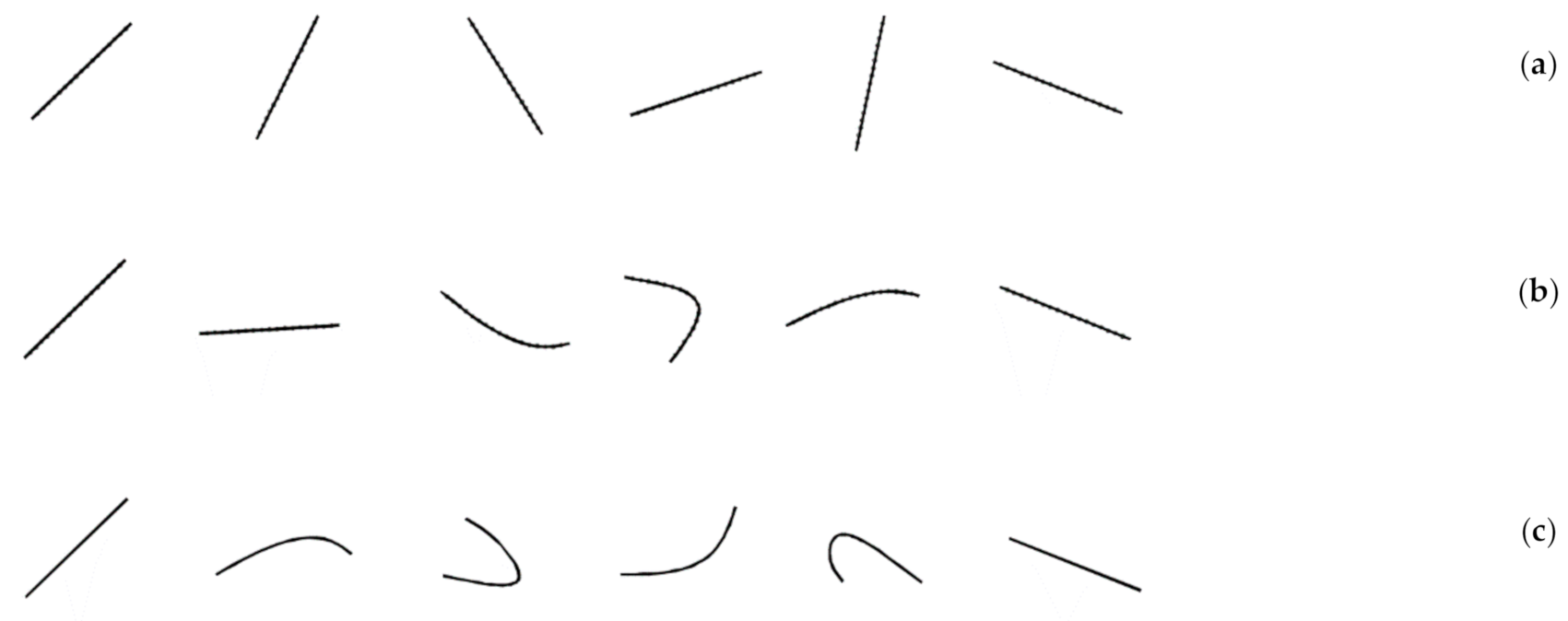
Regarding the flexible fibres, the effect of the dimensionless shear rate, is studied on the flexibility of a single fibre with 18 spheroids and an aspect ratio of 20. By changing three different values, 3.2 × 10⁻³, 7.2 × 10⁻⁴, and 1.43 × 10⁻⁴, the variety of complex rotational motions and flexibility of the fibre, reported by Forgacs and Mason [19], is investigated (Figure 7).
As shown in Figure 7a, at 1.43 × 10⁻⁴, the fibre plays a role as a rigid fibre and it rotates about its centre of mass. As the dimensionless shear rate, , increases, the fibre shows a flexible behaviour, and the end of the fibre deforms, as shown in Figure 7b. By increasing the dimensionless shear rate, 3.2 × 10⁻³, the S-shape flexibility that is reported by Forgacs and Mason [19] is observed (Figure 7c). Other research has reported similar results [8,32].
3. Results
Figure 8 shows the trajectory of a single rigid fibre past a cylinder. The fibre length and the cylinder diameter are similar, and the Reynolds number is 1. The fibre particle was set close to the horizontal centreline of the cylinder with a tilt angle equal to 10°. As the flow passes the fibre, it starts to rotate due to hydrodynamic forces applied on its segments. When it gets close enough to the cylinder, it starts rotating, and the maximum rotation would occur at an angle of 0°, where the flow velocity also has the maximum value. After this, the fibre starts passing the object and follows the flow streamlines. In the end, the fibre rests in the horizontal direction and leaves the cylinder. Aspect ratio is considered in this simulation.
Figure 9 shows a rigid long fibre passing a single cylinder, where the length of the fibre is 3D, and D is the cylinder diameter. The centre of gravity of the fibre is located off-centre of the cylinder horizontal centreline and is found to have unsymmetric hydrodynamic forces. Re = 1 and are considered for the flow Reynolds number and the aspect ratio of the fibre, respectively. As the flow passes the fibre, the applied forces push the fibre forward and it contacts with the cylinder. After that, the fibre slides over the cylinder and leaves it.
From Figure 8 and Figure 9, one can observe different behaviour of the single rigid fibre passing the cylinder. Examining several possibilities of the fibre position, we have focused only on the position where the centre of gravity of the fibre is located at the inflow centreline. In fact, we investigated the behaviour of the rigid and flexible fibres, where the flexibility of the fibre is varied by changing the dimensionless shear rate . In addition, the fibre initial angle of orientation is changed between 45° ≤ θ ≤ 75°. In all simulations, the Reynolds number is considered to be Re = 1. The aspect ratio is considered, and each fibre has six segments joints.
To observe the effect of fibre length, cylinder diameter, and the flexibility of the fibre on the movement of a single fibre, we consider two cases with different fibre length to cylinder diameter ratios (4 and 8). Initial orientation angle θ = 15°, 30°, and 45° and dimensioneless shear rate of , , and were considered for the fibre as well. An aspect ratio of is considered for both cases. The shorter case consists of 6 segments and the longer consist of 12 segments.
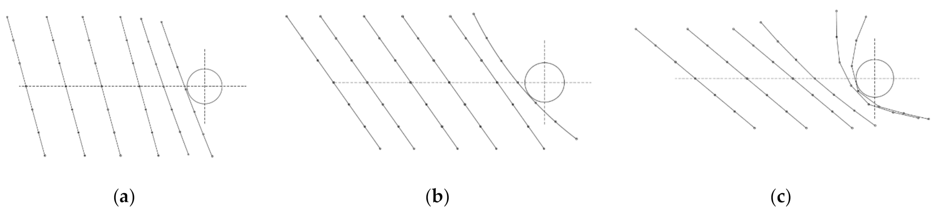
For the first case, the behaviour of a single fibre with three different flexibilities is observed, while the fibre initial orientation angle is varied. As shown in all plots in Figure 10, the fibre is carried by the flow, moves towards the cylinder, and touches the object. Depending on the rigidity of the fibre, the deformation of the cylinder can be varied. The fibre in Figure 10a is rigid, and its flexibility does not change when it contacts with the cylindrical object. For the other two fibres in Figure 10b,c, which are semi-flexible and fully flexible, the fibres deform. The initial orientation angle of the fibre has an important role of sliding off the fibre when the particle reaches the object. The larger the angle, the less sliding off can be observed in the figures. Even for the flexible fibre in Figure 10c, the inclination of the fibre can be seen when it reaches the cylindrical object. For the flexible fibre, bending of the fibre segment has been fully captured by the model as the fibre gets hung-up by the cylinder and all joints of the fibre segment react to the forces, and momentums is applied by the flow field around the cylindrical object.
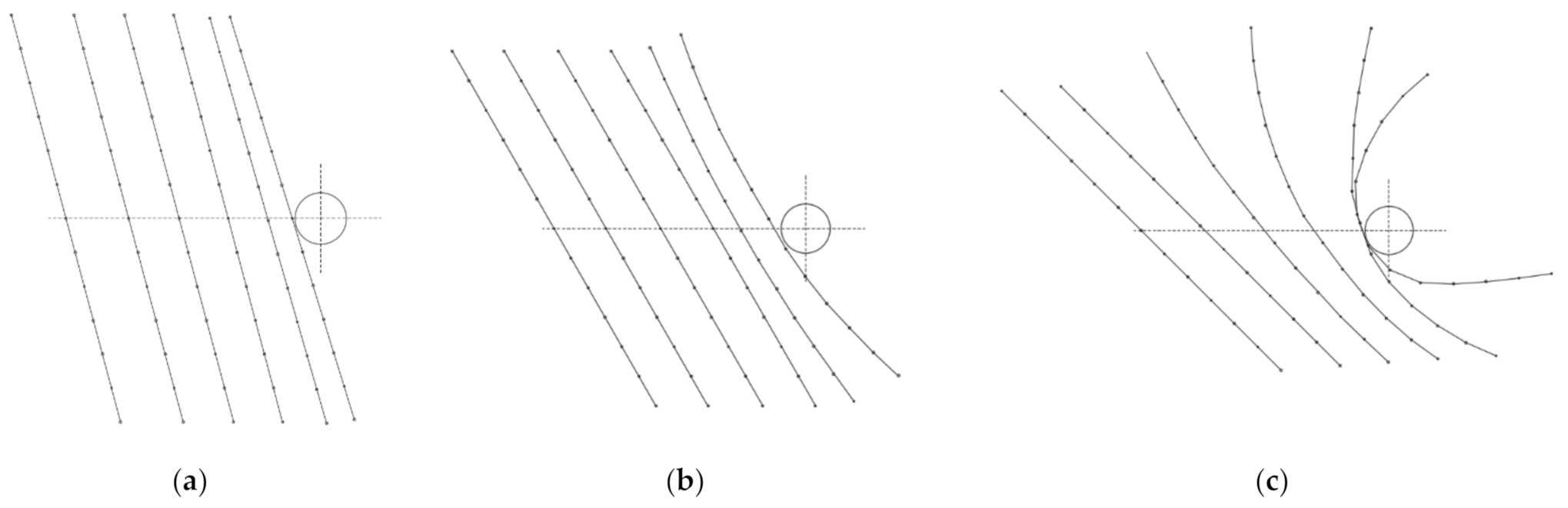
The behaviour of the single fibres in Figure 11 is physically expressible. Regarding the lowest dimensionless shear rate, , it is seen that, as soon as the fibre contacts with cylinder, it starts to incline until it leaves the domain.
4. Summary and Conclusions
The model of Ross and Klingenberg [32] was implemented in Open FOAM open source code, and the motion of a fibre was determined by solving the translational and rotational equations of motion for each spheroid segment. Translation, rotation, bending, and twisting were observed in the single flexible fibre motion. The model was validated against previous numerical and experimental benchmarks by Forgacs and Mason [19] and Jeffrey [35]. The flexibility of the fibre was expressed by the dimensionless shear rate, .
When a fibre slender particle is introduced to this flow field, the slender particle is oriented with is axes parallel to the principal axes of distortion of the fluid surrounding it. However, the vorticity tensor plays an opposite role and causes the slender body to adopt the same orientation as the surrounding fluid [34]. As expected, and as shown in Figure 10 and Figure 11, increasing the initial orientation angle would lead the fibre to be placed more in the flow direction. In fact, the distribution of a single fibre depends on the flow field and the interaction between the fibre and the single cylinder. The fibre interaction includes hydrodynamic and mechanical effects. Regarding the motion of the fibre, it is worth noting that, by increasing the initial orientation angle, the centroid of the fibre significantly moves downward. By increasing the flexibility of the fibre, this movement would decrease.
It should be emphasized here that by increasing the flexibility of the fibre, more rotation can be observed for the fibre when it is getting close to the cylinder. In other words, the interaction forces play significant roles on the rotation and movement of the fibre downward.
Simultaneously changing the fibre length and the fibre flexibility would increase the inter particle forces and momentums, and the fibre deformation would be seen more in the region close the cylinder.
Having various dimensionless shear rate values, different fibre configurations have been captured from fully rigid to full flexible fibres. After validating the implemented model, the behaviour of a single fibre with a different orientation angle, length, and flexibility is investigated around a single cylindrical object. It is shown that the initial orientation angle of the fibre has an influence on the flexibility and the shape of the fibre when it contacts with the cylinder. The model and the results can be employed to understand the behaviour of fibre suspension fluids in many applications such as lubrication and manufacturing processes.
Author Contributions
Conceptualization, N.H. and L.-G.W.; Methodology, N.H.; Software, N.H.; Validation, N.H.; Formal Analysis, N.H.; Investigation, L.-G.W.; Resources, L.-G.W.; Data Curation, N.H.; Writing–Original Draft Preparation, N.H.; Writing–Review & Editing, N.H. and L.-G.W.; Visualization, N.H.; Project Administration, L.-G.W.; Funding Acquisition, L.-G.W. All authors have read and agreed to the published version of the manuscript.
Funding
This research was funded by Swedish KEMPE Foundations, Grant Number SMK-1739.
Data Availability Statement
Data is contained within the article.
Acknowledgments
This research was conducted using the resources of High-Performance Computer Center North (HPC2N), Sweden.
Conflicts of Interest
The authors declare no conflict of interest.
References
- Yamamoto, S.; Matsuoka, T. Dynamic simulation of fiber suspensions in shear flow. J. Chem. Phys. 1995, 102, 2254–2260. [Google Scholar] [CrossRef]
- Yamamoto, S.; Matsuoka, T. A method for dynamic simulation of rigid and flexible fibers in a flow field. J. Chem. Phys. 1993, 98, 644–650. [Google Scholar] [CrossRef]
- Yamamoto, S.; Matsuoka, T. Viscosity of dilute suspensions of rodlike particles: A numerical simulation method. J. Chem. Phys. 1994, 100, 3317–3324. [Google Scholar] [CrossRef]
- Schmid, C.F.; Switzer, L.H.; Klingenberg, D.J. Simulations of fiber flocculation: Effects of fiber properties and interfiber friction. J. Rheol. 2000, 44, 781–809. [Google Scholar] [CrossRef] [Green Version]
- Lindström, S.B.; Uesaka, T. Simulation of the motion of flexible fibers in viscous fluid flow. Phys. Fluids 2007, 19, 113307. [Google Scholar] [CrossRef]
- Yamanoi, M.; Maia, J.; Kwak, T.-S. Analysis of rheological properties of fibre suspensions in a Newtonian fluid by direct fibre simulation. Part 2: Flexible fibre suspensions. J. Non Newton. Fluid Mech. 2010, 165, 1064–1071. [Google Scholar] [CrossRef]
- Yamanoi, M.; Maia, J.M. Analysis of rheological properties of fibre suspensions in a Newtonian fluid by direct fibre sim-ulation. Part1: Rigid fibre suspensions. J. Non Newton. Fluid Mech. 2010, 165, 1055–1063. [Google Scholar] [CrossRef]
- Andrić, J.; Lindström, S.B.; Sasic, S.; Nilsson, H. Rheological properties of dilute suspensions of rigid and flexible fibers. J. Non Newton. Fluid Mech. 2014, 212, 36–46. [Google Scholar] [CrossRef]
- Switzer, L.H.; Klingenberg, D.J. Rheology of sheared flexible fiber suspensions via fiber-level simulations. J. Rheol. 2003, 47, 759–778. [Google Scholar] [CrossRef] [Green Version]
- Redlinger-Pohn, J.D.; König, L.M.; Kloss, C.; Goniva, C.; Radl, S.; Papadrakakis, M. Modelling of Non-Spherical, Elongated Particles for Industrial Suspension Flow Simulation. In Proceedings of the VII European Congress on Computational Methods in Applied Sciences and Engineering, Crete Island, Greece, 5–10 June 2016. [Google Scholar]
- Sasic, S.; Almstedt, A.-E. Dynamics of fibres in a turbulent flow field–A particle-level simulation technique. Int. J. Heat Fluid Flow 2010, 31, 1058–1064. [Google Scholar] [CrossRef]
- Guo, H.; Xua, B. A novel method for dynamic simulation of flexible fibers in a 3D swirling flow. Int. J. Nonlinear Sci. Numer. Simul. 2009, 10, 1473–1480. [Google Scholar] [CrossRef]
- Delmotte, B.; Climent, E.; Plouraboué, F. A general formulation of bead models applied to flexible fibers and active fila-ments at low Reynolds number. J. Comput. Phys. 2015, 286, 14–37. [Google Scholar]
- MacMeccan, R.M.; Clausen, J.R.; Neitzel, G.P.; Aidun, C.K. Simulating deformable particle suspensions using a coupled lattice-Boltzmann and fi-nite-element method. J. Fluid Mech. 2009, 618, 13–39. [Google Scholar] [CrossRef]
- Qi, D. Direct simulations of flexible cylindrical fiber suspensions in finite Reynolds number flows. J. Chem. Phys. 2006, 125, 114901. [Google Scholar] [CrossRef] [PubMed]
- Peskin, C.S. Numerical analysis of blood flow in the heart. J. Comput. Phys. 1977, 25, 220–252. [Google Scholar] [CrossRef]
- Chaouche, M.; Koch, D.L. Rheology of non-Brownian rigid fiber suspensions with adhesive contacts. J. Rheol. 2001, 45, 369–382. [Google Scholar] [CrossRef]
- Yasuda, K.; Henmi, S.; Mori, N. Effects of abrupt expansion geometries on flow-induced fiber orientation and concen-tration distributions in slit channel flows of fiber suspensions. Polym. Compos. 2005, 26, 660–670. [Google Scholar] [CrossRef]
- Forgacs, O.; Mason, S. Particle motions in sheared suspensions: X. Orbits of flexible threadlike particles. J. Col. Loid. Sci. 1959, 14, 473–491. [Google Scholar] [CrossRef]
- Arlov, A.; Forgacs, O.; Mason, S. Particle motions in sheared suspensions IV. General behaviour of wood pulp fibres. Sven. Papp. 1958, 61, 61–67. [Google Scholar]
- Sepehr, M.; Carreau, P.J.; Moan, M.; Ausias, G. Rheological properties of short fiber model suspensions. J. Rheol. 2004, 48, 1023–1048. [Google Scholar] [CrossRef]
- Switzer, L.H.; Klingenberg, D.J. Simulations of fiber floc dispersion in linear flow fields. Nord. Pulp Pap. Res. J. 2003, 18, 141–144. [Google Scholar] [CrossRef]
- Yasuda, K.; Kyuto, T.; Mori, N. An experimental study of flow-induced fiber orientation and concentration distributions in a concentrated suspension flow through a slit channel containing a cylinder. Rheol. Acta 2004, 43, 137–145. [Google Scholar] [CrossRef]
- Vakil, A.; Green, S. Two-dimensional side-by-side circular cylinders at moderate Reynolds numbers. Comput. Fluids 2011, 51, 136–144. [Google Scholar] [CrossRef]
- Forgacs, O. The hydrodynamic behaviour of papermaking fibres. Fundam. Papermak. Fibres 1958, 447, 37. [Google Scholar]
- Bharti, R.; Chhabra, R.P.; Eswaran, V. Steady Flow of Power Law Fluids across a Circular Cylinder. Can. J. Chem. Eng. 2008, 84, 406–421. [Google Scholar] [CrossRef]
- Chakraborty, J.; Verma, N.; Chhabra, R.P. Wall effects in flow past a circular cylinder in a plane channel: A numerical study. Chem. Eng. Process. Process. Intensif. 2004, 43, 1529–1537. [Google Scholar] [CrossRef]
- Niu, X.; Chew, Y.; Shu, C. Simulation of flows around an impulsively started circular cylinder by Taylor series expan-sion-and least squares-based lattice Boltzmann method. J. Comput. Phys. 2003, 188, 176–193. [Google Scholar] [CrossRef]
- Park, J.; Kwon, K.; Choi, H. Numerical solutions of flow past a circular cylinder at Reynolds numbers up to 160. KSME Int. J. 1998, 12, 1200–1205. [Google Scholar] [CrossRef]
- Dennis, S.C.R.; Chang, G.-Z. Numerical solutions for steady flow past a circular cylinder at Reynolds numbers up to 100. J. Fluid Mech. 1970, 42, 471–489. [Google Scholar] [CrossRef]
- Fornberg, B. A numerical study of steady viscous flow past a circular cylinder. J. Fluid Mech. 1980, 98, 819–855. [Google Scholar] [CrossRef] [Green Version]
- Ross, R.F.; Klingenberg, D.J. Dynamic simulation of flexible fibers composed of linked rigid bodies. J. Chem. Phys. 1997, 106, 2949–2960. [Google Scholar] [CrossRef] [Green Version]
- Weller, H.G.; Tabor, G.; Jasak, H.; Fureby, C. A tensorial approach to computational continuum mechanics using object-oriented techniques. Comput. Phys. 1998, 12, 620–631. [Google Scholar] [CrossRef]
- Kim, S.; Karrila, S.J. Microhydrodynamics: Principles and Selected Applications; Courier Corporation: Chelmsford, MA, USA, 2013. [Google Scholar]
- Jeffery, G.B. The motion of ellipsoidal particles immersed in a viscous fluid. Proc. R. Soc. Lond. Ser. A Contain. Pap. Math. Phys. Character 1922, 102, 161–179. [Google Scholar] [CrossRef] [Green Version]
Figure 1.
Problem setup and arrangement for the cylinder in the channel.

Figure 2.
(a) Discretized model for the single cylinder, (b) a closer view of the grid for the single cylinder.
Figure 2.
(a) Discretized model for the single cylinder, (b) a closer view of the grid for the single cylinder.

Figure 3.
Flow field around a single cylinder, (a) velocity magnitude field, (b) Shear strain rate field.
Figure 3.
Flow field around a single cylinder, (a) velocity magnitude field, (b) Shear strain rate field.

Figure 4.
Illustration of multiple spheroids as a model of a single fibre.

Figure 5.
Applied forces and torques on a single sphroid, i.

Figure 6.
Validation of the implemented spheroid fibre model against Jeffrey orbit theory [35] and Forgacs and Mason [19].

Figure 7.
Time sequence of images from the simulation for various dimensionless shear rates: (a) , (b) , and (c) .
Figure 7.
Time sequence of images from the simulation for various dimensionless shear rates: (a) , (b) , and (c) .

Figure 8.
Trajectory of a single rigid fibre with six segments around a cylinder where the fibre length and cylinder diameter are the same.
Figure 8.
Trajectory of a single rigid fibre with six segments around a cylinder where the fibre length and cylinder diameter are the same.

Figure 9.
Trajectory of a single rigid fibre with six segments around a cylinder where the fibre length is 3D.
Figure 9.
Trajectory of a single rigid fibre with six segments around a cylinder where the fibre length is 3D.

Figure 10.
Movement of a single fibre past a cylinder where the ratio of the fibre length to the cylinder diameter is 4: (a) , θ = 15°, (b) , θ = 30°, (c) , θ = 45°.
Figure 10.
Movement of a single fibre past a cylinder where the ratio of the fibre length to the cylinder diameter is 4: (a) , θ = 15°, (b) , θ = 30°, (c) , θ = 45°.

Figure 11.
Movement of a single fibre past a cylinder where the ratio of the fibre length to the cylinder diameter is 8: (a) , θ = 15°, (b) , θ = 30°, (c) , θ = 45°.
Figure 11.
Movement of a single fibre past a cylinder where the ratio of the fibre length to the cylinder diameter is 8: (a) , θ = 15°, (b) , θ = 30°, (c) , θ = 45°.


Table 1.
Drag variation for various Reynolds numbers in the current study compared to previous works.
Table 1.
Drag variation for various Reynolds numbers in the current study compared to previous works.
| Reference | Re = 20 | Re = 40 |
|---|---|---|
| Present work | 1.9999 | 1.4998 |
| Bharti et al. [26] | 2.0455 | 1.5292 |
| Chakraborty et al. [27] | 2.0223 | 1.5172 |
| Niu et al. [28] | 2.1110 | 1.5740 |
| Park et al. [29] | 2.0100 | 1.5100 |
| Dennis and Chang [30] | 2.0450 | 1.5220 |
| Fornberg [31] | 2.0000 | 1.4980 |
Publisher’s Note: MDPI stays neutral with regard to jurisdictional claims in published maps and institutional affiliations. |
© 2021 by the authors. Licensee MDPI, Basel, Switzerland. This article is an open access article distributed under the terms and conditions of the Creative Commons Attribution (CC BY) license (http://creativecommons.org/licenses/by/4.0/).
Share and Cite
MDPI and ACS Style
Hamedi, N.; Westerberg, L.-G. Simulation of Flexible Fibre Particle Interaction with a Single Cylinder. Processes 2021, 9, 191. https://doi.org/10.3390/pr9020191
AMA Style
Hamedi N, Westerberg L-G. Simulation of Flexible Fibre Particle Interaction with a Single Cylinder. Processes. 2021; 9(2):191. https://doi.org/10.3390/pr9020191
Chicago/Turabian StyleHamedi, Naser, and Lars-Göran Westerberg. 2021. "Simulation of Flexible Fibre Particle Interaction with a Single Cylinder" Processes 9, no. 2: 191. https://doi.org/10.3390/pr9020191
Note that from the first issue of 2016, this journal uses article numbers instead of page numbers. See further details here.