
New Metallic Damper with Multiphase Behavior for Seismic Protection of Structures


Department of Mechanical Engineering, Universidad Politécnica de Madrid, 28006 Madrid, Spain
*
Author to whom correspondence should be addressed.
Metals 2021, 11(2), 183; https://doi.org/10.3390/met11020183
Submission received: 1 January 2021
/
Revised: 13 January 2021
/
Accepted: 19 January 2021
/
Published: 20 January 2021
(This article belongs to the Special Issue Advances in Structural Steel Research)
Abstract
:This paper proposes a new metallic damper based on the plastic deformation of mild steel. It is intended to function as an energy dissipation device in structures subjected to severe or extreme earthquakes. The damper possesses a gap mechanism that prevents high-cycle fatigue damage under wind loads. Furthermore, subjected to large deformations, the damper presents a reserve of strength and energy dissipation capacity that can be mobilized in the event of extreme ground motions. An extensive experimental investigation was conducted, including static cyclic tests of the damper isolated from the structure, and dynamic shake-table tests of the dampers installed in a reinforced concrete structure. Four phases are distinguished in the response. Based on the results of the tests, a hysteretic model for predicting the force-displacement curve of the damper under arbitrary cyclic loadings is presented. The model accurately captures the increment of stiffness and strength under very large deformations. The ultimate energy dissipation capacity of the damper is found to differ depending on the phase in which it fails, and new equations are proposed for its prediction. It is concluded that the damper has a stable hysteretic response, and that the cyclic behavior, the ultimate energy dissipation capacity and failure are highly predictable with a relatively simple numerical model.
1. Introduction
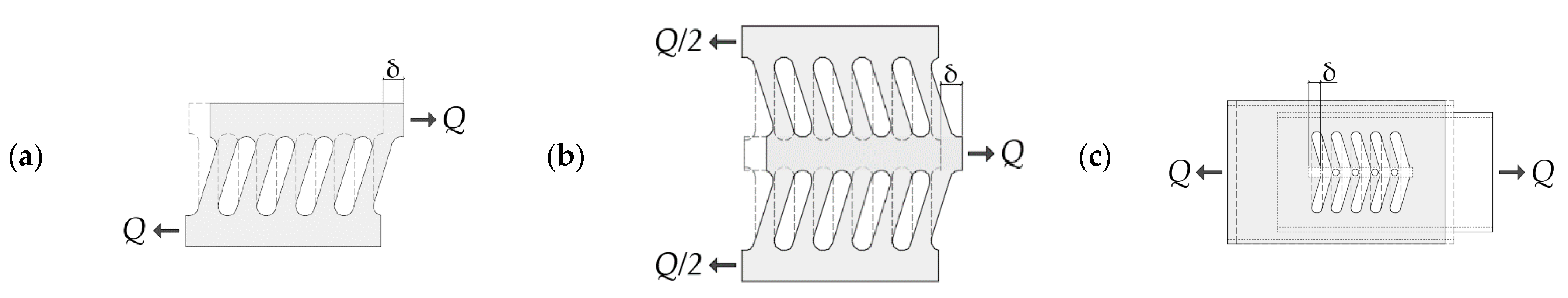
The 1994 Northridge (California) and 1995 Kobe (Japan) earthquakes highlighted that a conventional seismic design—where the beams and columns of the main structure are designed to dissipate energy through plastic deformations under a severe ground motion—results in significant structural and nonstructural damage and the interruption of a building’s use after the event. Since the beginning of the 21st century, seismic engineering has undergone a transition toward so-called Performance-Based Design (PBD), aimed at controlling/minimizing the consequent damage and financial losses. Structures with energy dissipation systems have proven to be a very effective solution to attain the objectives of PBD. They consist of a main structure that supports the gravity loads and an energy dissipation system working in parallel. The latter is formed by special structural elements called energy dissipation devices (EDDs), or simply dampers, plus the auxiliary elements that connect the EDDs with the main structure. The EDDs are in charge of absorbing most of the energy input by the earthquake, releasing the main structural elements from dissipating energy through plastic deformations. During the earthquake, the response of the main structure is essentially elastic, and at the end of the event it is basically undamaged. The damage concentrates in the EDDS, which is purposely designed to be easily inspected, replaced or repaired after a severe (commonly called “design earthquake”) or an extreme (“maximum credible earthquake”) ground motion. This allows for the continuous use of a building without interruption, enhancing resilience. Since its first application in the early 1970s [1], the addition of EDDs has proven to be an effective technology for the seismic protection of buildings. EDDs can be classified as either displacement-dependent or velocity-dependent. The former includes metallic dampers (also called hysteretic dampers) and friction dampers [2,3,4,5]. This paper is focused on metallic EDDs, whose source of energy dissipation is the yielding of metals [6]. They are built with well-known and reliable material (mild steel) that have a stable hysteretic behavior and a large inherent plastic deformation capacity. A comprehensive state-of-art review of the development and implementation of metallic EDDs can be found in [7]. Different types of metallic EDDs have been proposed in the literature and used in practical applications. Among the most popular are the Added Damping and Stiffness damper (ADAS) [8] and its triangular version (TADAS) [9], the buckling restrained brace [10], or the steel plate with slits [11], also called slit-type damper herein. The latter consists of strips of steel having constant or variable width, made by opening slits—either simple (Figure 1a) or double (Figure 1b)—in a steel plate. The mechanism for energy dissipation resides in plastic bending/shearing deformations of the steel strips.
The slit-type damper has been successfully implemented in actual building designs such as the Sapporo Hotel in Japan [12] and several studies have been carried out over the last decade. Chan and Albermani [6] proposed a slit-type damper that is fabricated from a standard structural wide-flange section by opening slits in the web. Oh et al. [13] verified through cyclic tests the seismic performance of steel structures with slit-type dampers at the bottom flange and confirmed their satisfactory performance. Striving to optimize the EDD, Ghabraie et al. [14] and Zheng et al. [15] investigated new shapes for the steel strips (i.e., with a variable section) to enhance their energy dissipation capacity. Lee et al. [16] tested the cyclic performance of three different shapes in order to reduce stress concentration: dumbbell-shaped strip, tapered strip and hourglass-shaped strip. Amiri et al. [17] studied a block slit damper with a very low height-to-thickness ratio. Shao et al. [18] investigated the double slit configurations (spine) shown in Figure 1b. Benavent–Climent [19] proposed a tube-in-tube damper based on flexural/shear yielding of the steel strips formed by opening slits on the walls of hollow structural sections (Figure 1c). A similar concept was applied by Lee and Kim [20], who proposed a box-shaped steel slit damper. In the last ten years, hybrid dampers that use two different passive elements combined in a single device have been proposed, e.g., viscoelastic dampers and metallic dampers [21], or friction dampers and metallic dampers [22]. Nowadays, a limited body of work exists for hybrid dampers, but it is an interesting solution that receives increasing attention [23].
Metallic dampers are conceived to dissipate energy through plastic deformations in case of severe earthquakes. However, under wind loads, they are subjected to thousands of cycles within the elastic range that can cause high cycle fatigue damage, compromising the efficiency of the damper against the main shock. This problem is not exclusive of metallic dampers; it affects steel structures in general [24]. In the past, high cycle fatigue due to wind loads has caused severe damage or even collapse in steel elements such as cantilever steel structures or poles [25]. Low-to-mid-rise buildings designed following modern codes are generally stiff enough to render the dynamic response induced by the wind as negligible, so that it can be endured by the main structure with no need for dampers [26]. This paper presents a new damper that avoids the problem of high cycle fatigue by introducing a gap mechanism. The proposed damper is intended to be used in low-to-mid-rise buildings (up to about 12 floors) designed following modern codes, that can endure wind loads with no need for braces.
Another characteristic feature of most metallic dampers is that beyond a given displacement (typically large), they present a significant increase of the restoring force and plastic stiffness. In the case of the slit-type damper, this occurs when the displacement of the ends of the steel strip in the direction of its axis are restrained. This restriction gives rise to important axial forces in the steel strips (in addition to bending and shear forces), that result in the aforementioned significant increase of the restoring force and stiffness. This is not exclusive of slit-type dampers; it occurs with other types of metallic dampers (e.g., the TADAS damper [9]) and can be prevented using appropriate connections (e.g., using pin-connections and slotted holes) at the expense of incrementing the production cost of the damper. The increment of restoring forces at large displacements can be considered as a flaw from the standpoint of the additional forces that this overstrength imposes upon the main structure and foundation. Yet if it is anticipated on design, and the main structure is prepared for it, it may prove beneficial as a reserve of strength and energy dissipation capacity, being necessary in the case of an extremely high amplitude earthquake. In fact, as shown later in this paper, the reserve of energy dissipation capacity of the damper is very large when the restoring force starts to increase significantly until failure. An additional reason why this increase in the restoring force under large displacements is often ignored is that it cannot be easily captured by the numerical models typically used to characterize the hysteretic behaviour of metallic dampers (i.e., the Bouc–Wen model). This paper presents a simple numerical model that can accurately reproduce the increment of restoring force at large displacements, as well as the amount of dissipated energy, and predict the force displacement hysteretic curves of the metallic damper under arbitrarily applied cyclic loading until failure.
2. Design Concept of the New Metallic Damper and Materialization
2.1. Design Concept
The concept of the metallic EDD investigated in this study is depicted in Figure 2 and will be called herein the Multi-Phased Tube-in-Tube Damper (MP-TTD). It consists of two tubes arranged in a telescopic configuration that can be installed in the main structure as conventional brace/diagonal members. Two faces of the outer tube are slitted to form two rows of steel strips that constitute the part of the device that undergoes plastic deformation. The damper is suitable for easy transformation into a hybrid damper by inserting a viscoelastic material between the tubes, in the two faces of the outer tube that are not slitted (Figure 2a). Investigation of this latter possibility lies beyond the scope of the present paper, which instead focuses on the metallic damper that uses the plastic deformation of the steel strips as a source of energy dissipation.
To safeguard the metallic damper from high cycle fatigue damage when subjected to wind loads, a mechanical gap is introduced; it avoids plastic deformations on the steel strips within the range of building displacements below the gap width . The metallic damper has a multiphase nature. For displacements along the axis of the damper below , the damper is not activated and will be referred to as Phase I herein. Beyond Phase I, the damper is activated and exhibits three additional phases. Phase II occurs between and the yield displacement in which the damper only provides stiffness and stores elastic strain energy. Phase III would be between and the displacement associated with the onset of the in which the damper provides stiffness and plastic strain energy dissipation capacity at a nearly constant force. Finally, in Phase IV beyond the damper increases both stiffness and strength significantly, while dissipating energy through plastic deformations. The displacements associated with the transition from one phase to the following can be determined upon design by using appropriate values for , for the geometry and number of steel strips and for the geometry of the outer tube. The values of the displacements can be tuned so that under wind loads the damper’s response is within Phase I, under moderate (frequent) earthquakes it does not exceed Phase II, under a severe (“design earthquake”) motion the response does not go beyond Phase III, and under a rare (“maximum credible earthquake”) ground motion the damper enters Phase IV.
2.2. Materialization
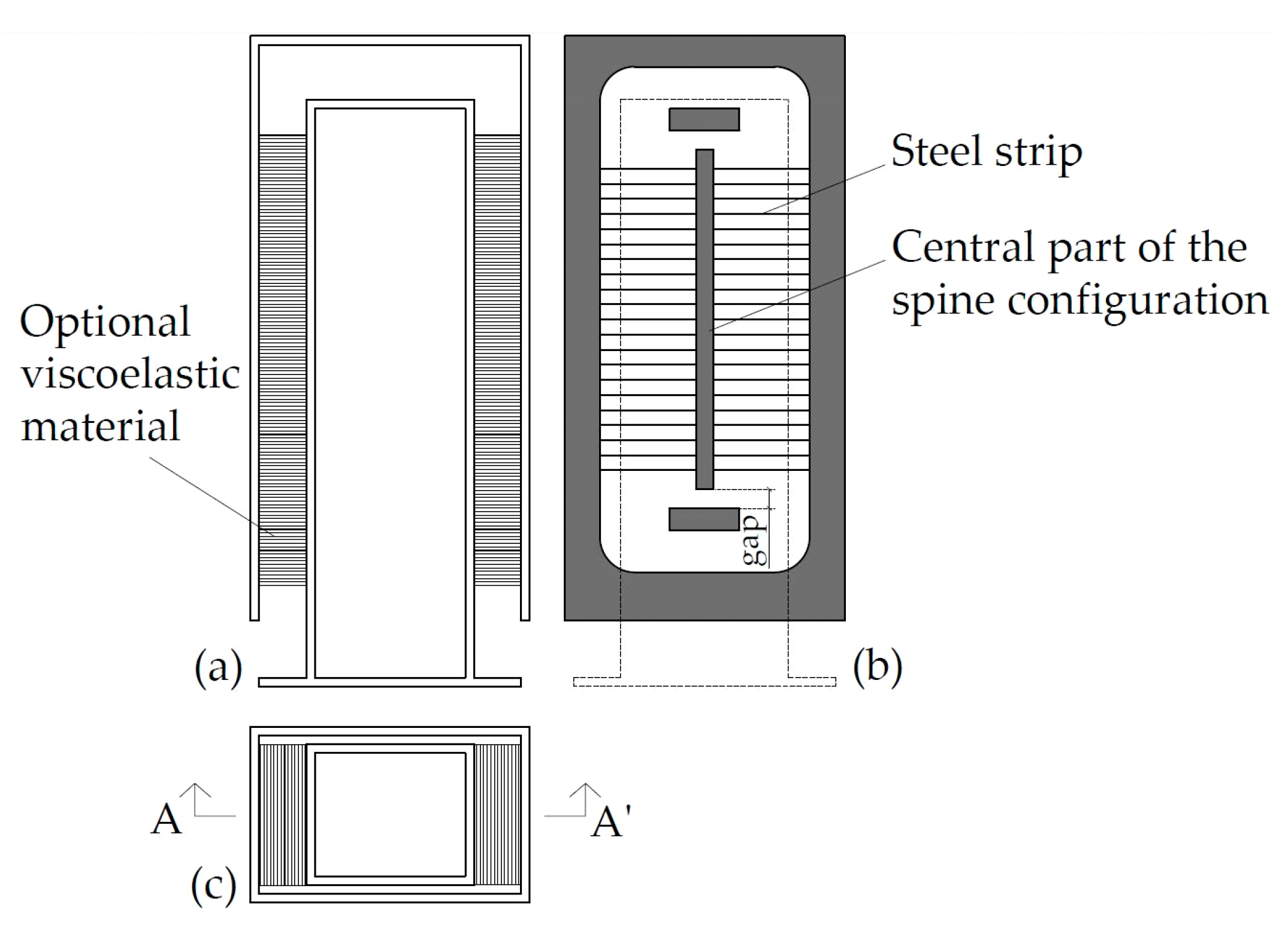
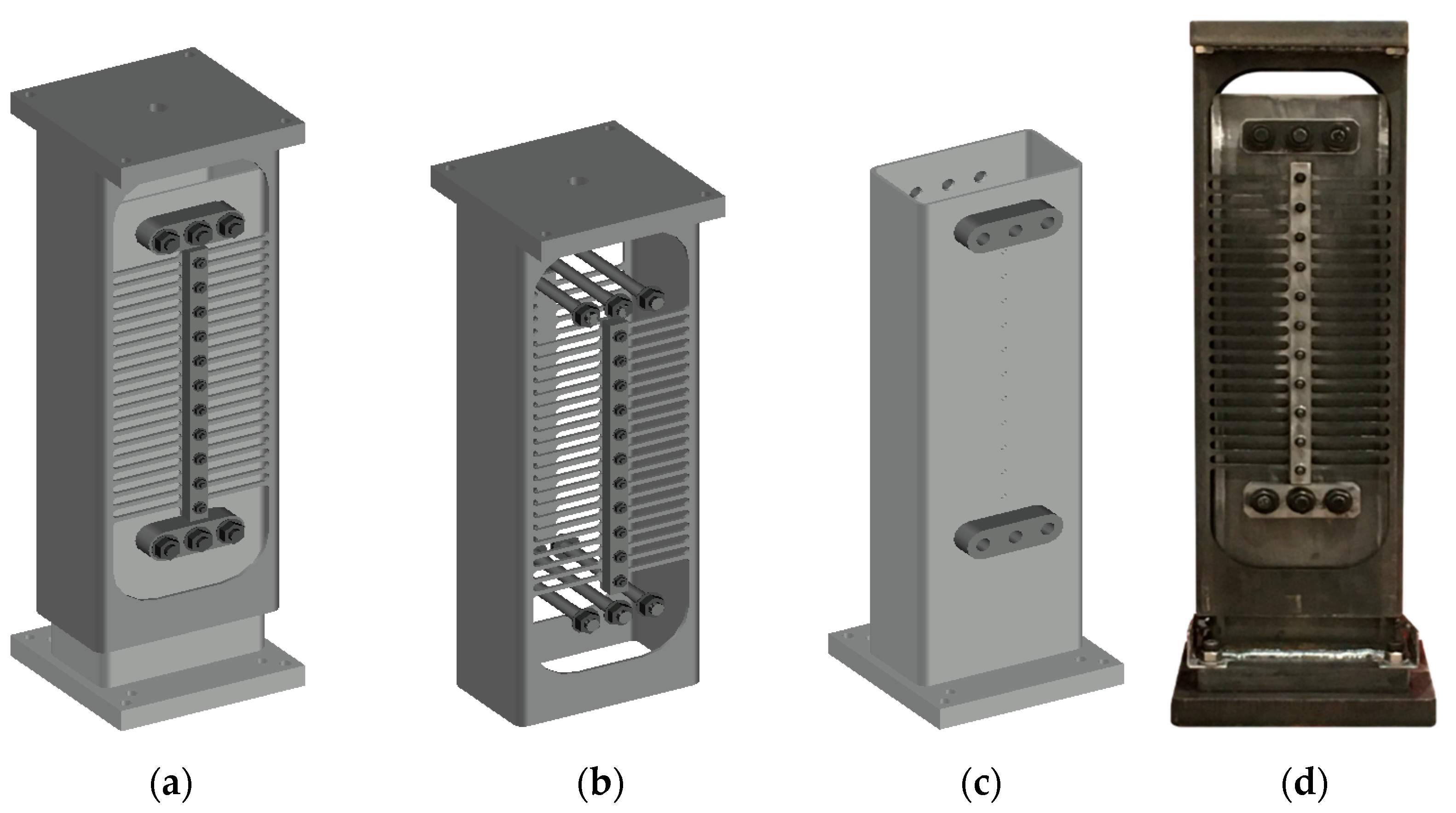
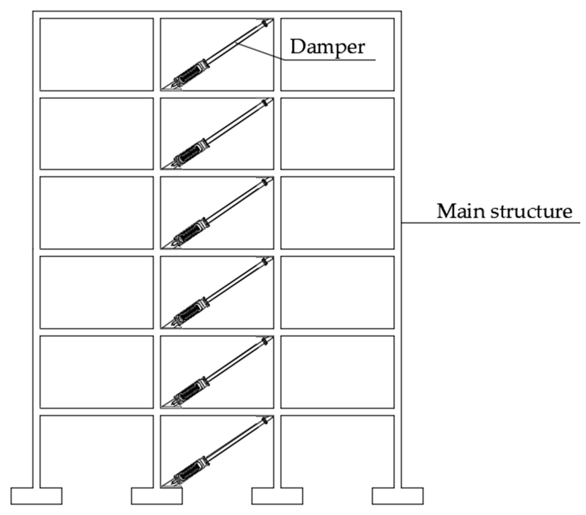
The design concept explained above is materialized in the metallic damper shown in Figure 3a. It is made of two standard hollow structural sections. In two faces of the outer tube (Figure 3b), slotted holes are opened using a waterjet cutting system in order to have smooth finished surfaces and to prevent altering the properties of the steel by heat. The steel strips between the slotted holes have a spinal configuration. To prevent out-of-plane buckling of the strips, the central part of the spine is strengthened with a rectangular plate fixed with pre-stressed high strength bolts to the outer tube. The inner tube (Figure 3c) has four stoppers fixed with high strength steel rods that are post-tensioned in order to avoid any slippage of the stopper with respect to the inner tube. The well-pondered location of these stoppers allows for the gap . Figure 3d offers a photo of the metallic dampers used in the test campaign explained next. Figure 4 reflects the implementation of the metallic damper in a frame structure.
3. Experimental Research
The performance of seven identical MP-TTD specimens, referred to as MP-TTD -0 to MP-TTD-6 herein, up to failure was studied experimentally under quasi-static cyclic tests, dynamic seismic shake table tests, and a mixture of dynamic plus quasi-static tests. For all test types, failure was assumed to occur when the restoring force opposed by the damper started to decrease under increasing imposed deformations.
Specimen MP-TTD-0 was tested isolated from the structure under quasi-static cyclic loadings. Specimens MP-TTD-1 to MP-TTD-6 were installed in a reinforced concrete (RC) structure that was subjected to realistic seismic loadings on a shake table. During the dynamic shake table tests, specimens MP-TTD-2 and MP-TTD-3 reached failure, specimens MP-TTD-1 and MP-TTD-4 suffered severe plastic deformations, and specimens MP-TTD-5 and MP-TTD-6 remained within the elastic range. After the dynamic shake table tests, specimens MP-TTD-1, MP-TTD-4, MP-TTD-5 and MP-TTD-6 were removed and isolated from the RC structure, then subjected to additional quasi static cyclic loading tests until failure.
3.1. Description of MP-TTDs Tested, Material Properties and Predicted Axial Strength and Yield Deformation
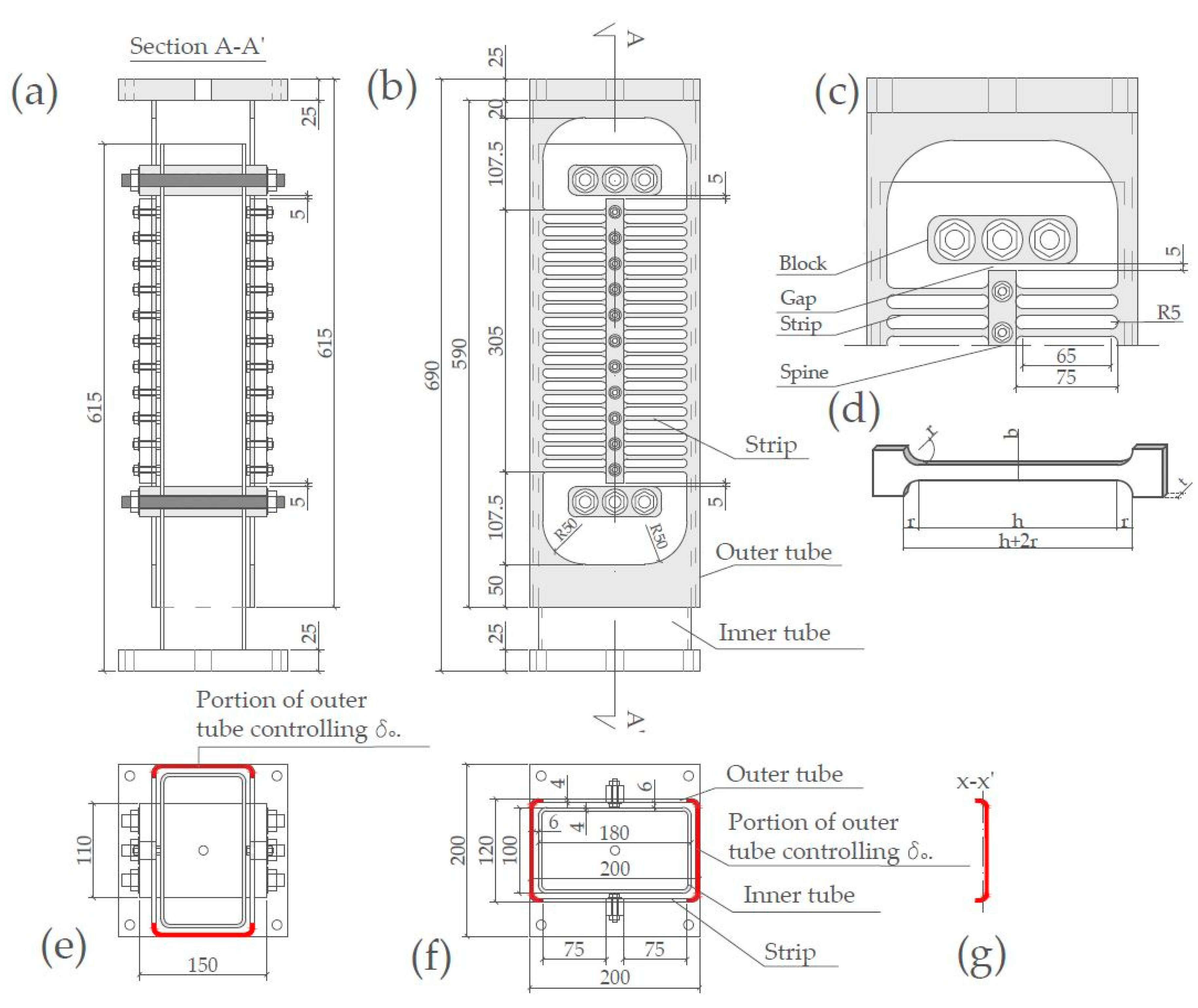
All dampers were made from the same hollow tubes in order to ensure identical characteristics for the steel. The nominal dimensions of the outer tube were #200.120.4 (width, depth, and thickness in mm), while the inner tube was #180.100.4. Figure 5 shows the geometry of the tested specimens, including detailed geometry of the steel strips. The specimens represent at a 2/5 scale the dampers that would be installed in a full-scale structure having 6500 mm span length and 3800 mm story height. As shown in Figure 5, the value selected for the gap was . The axial deformation in the scaled damper corresponds to an inter-story drift of 0.38%. This inter-story drift is smaller than the maximum value (about 0.5%) that typical reinforced concrete or steel structures can endure in the elastic range. Therefore, the scaled damper was designed with a gap of because typical structures can endure the lateral displacements associated with this gap without damage. In practical application, for fastening the assembly of the inner and outer tubes so that the two gaps are equal, the brace damper would be supplied with provisional and easily removable steel blocks that close the gap. These steel blocks would be removed once both ends of the brace damper are fixed to the main structure.
The steel class was S-275JR. The material properties were determined from three coupon tensile tests. Table 1 summarizes the mean Young modulus E, yield stress σy, ultimate stress σu, and the corresponding strains εy and εu.
Assuming that the ends of the steel strips are perfectly clamped (no rotation), and replacing the total height of the strip h + 2r (see Figure 5d) by an equivalent height h′ given by h′ = h + (2r2/(h + 2r)) to take into account the rounded ends [19]. The meanings of h (=65 mm) and r (=5 mm), are shown in the detail of the strip of Figure 5d. The mechanical properties of the MP-TTD can be predicted through simple mechanical principles. Considering an MP-TTD constituted of n steel strips, the force Q (see Figure 1b) when all fibers of the cross-section of the strips reach σy (referred to as yield strength Qy hereafter), and the force when all fibers of the cross-section reach σu, (referred to as strength QB herein) are given by [19]:
The meanings of t (= 4 mm) and b (= 5 mm) are shown in the detail of the strip of Figure 5d. The yield displacement of a MP-TTD with n steel strips can be estimated as follows [19]:
Using the material properties of Table 1 and the above equations, the predicted strengths and axial displacement of the specimens are Qy = 23.15 kN, QB = 33.89 kN and
3.2. Quasi-Static Tests
3.2.1. Experimental Set-Up and Loading Histories
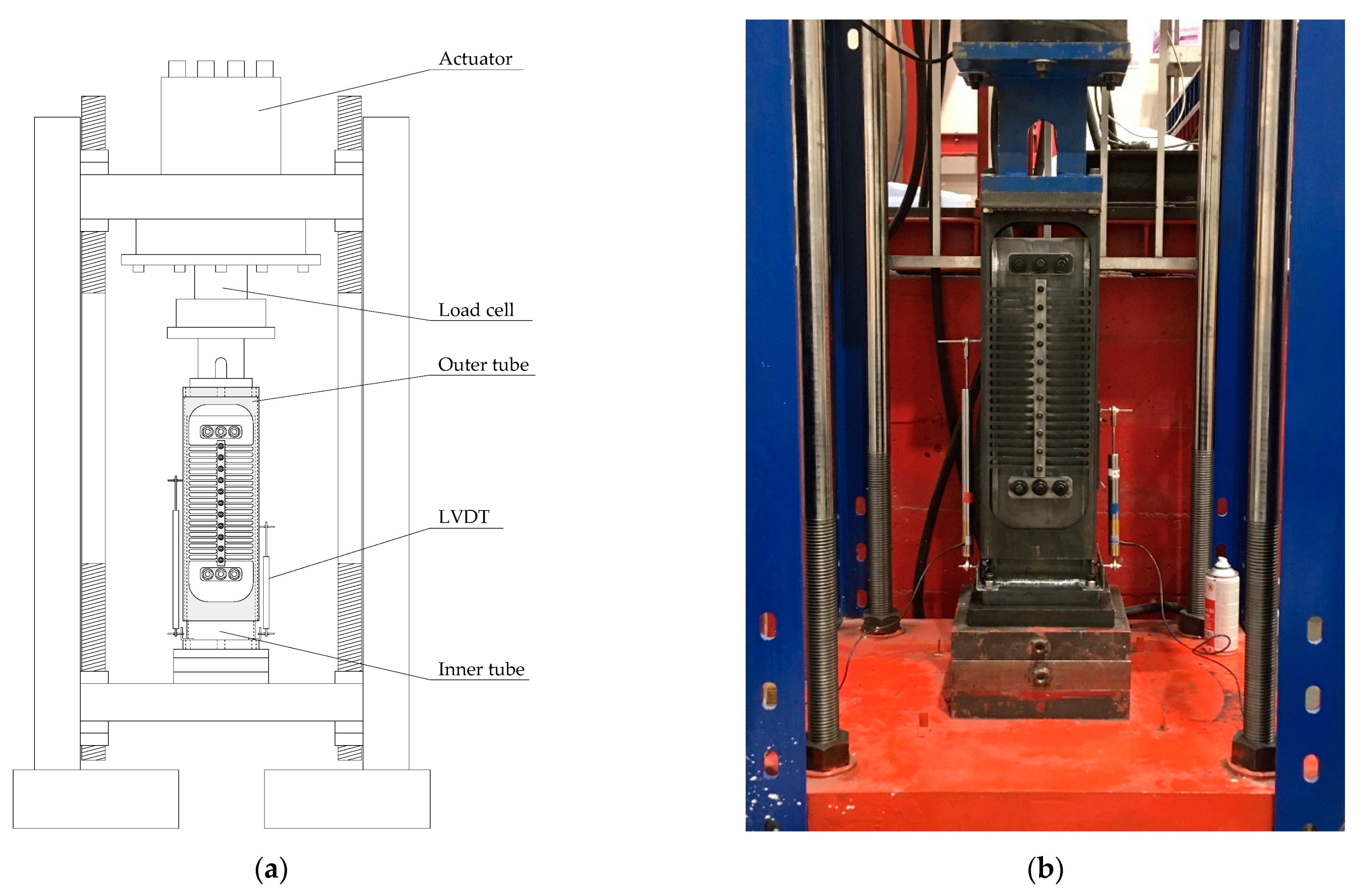
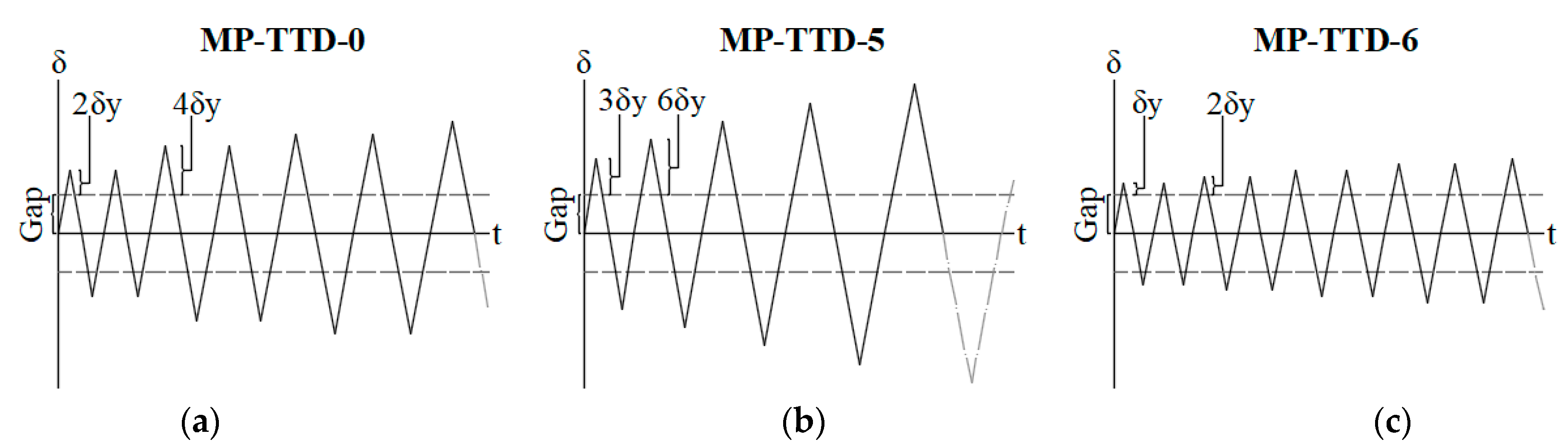
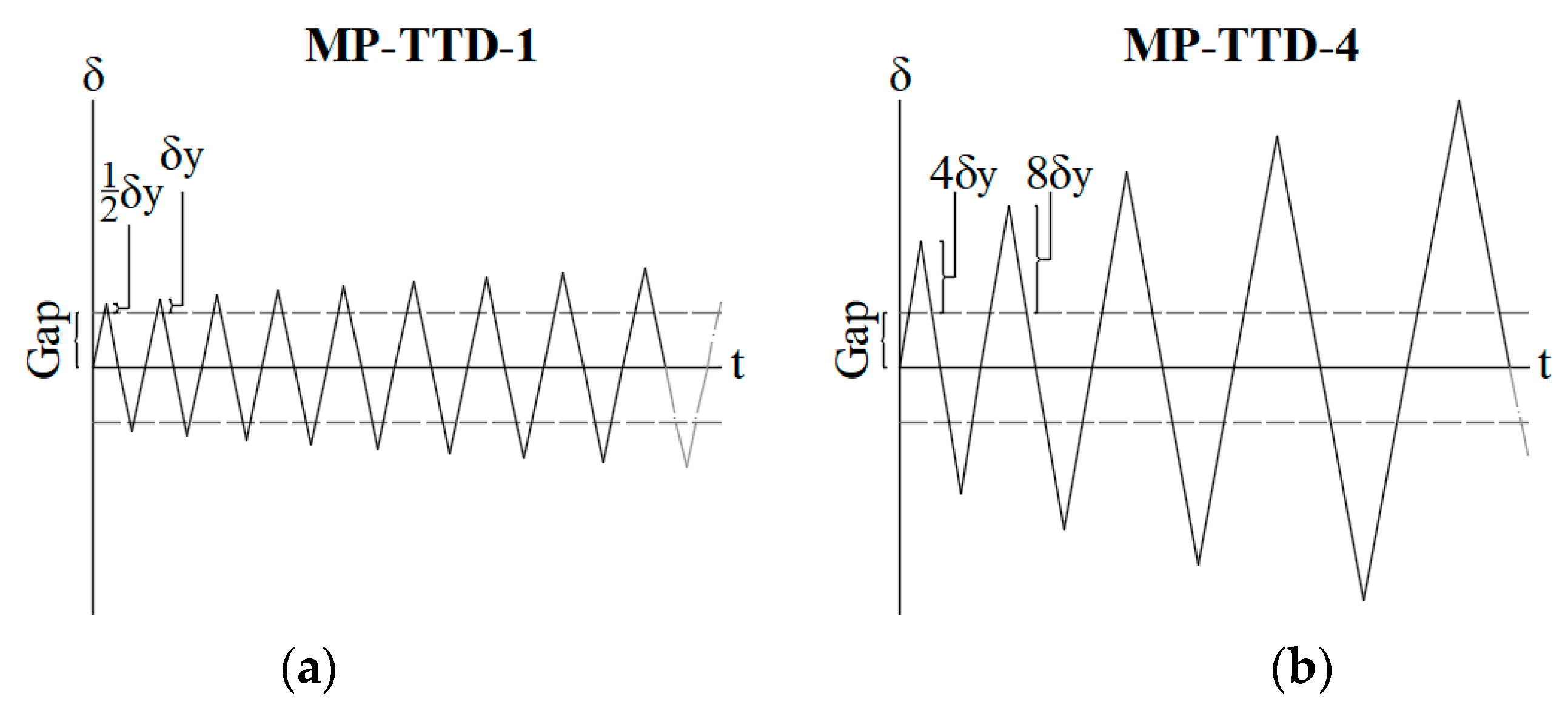
The hysteretic behavior and energy dissipation capacity of specimens MP-TTD-0, MP-TTD-5 and MP-TTD-6 were determined through quasi-static uniaxial cyclic tests conducted until failure. It is worth recalling that prior to the quasi-static tests, specimens MP-TTD-5 and MP-TTD-6 were subjected to dynamic loadings within the RC structure tested on the shake table, but the response was purely elastic and the number of cycles applied was far lower than that discussed in the high-cycle fatigue phenomena. Therefore, the energy dissipation capacity through plastic deformations of these two specimens is entirely obtained through quasi-static loadings. Figure 6a shows the test set-up. The tests were carried out using a universal testing machine SAXEWAY T1000 (MOOG Inc., East Aurora, NY, USA) with a maximum load capacity of 1000 kN (Figure 6b). For the tests, the inner tube was post-tensioned against the base of the apparatus, whereas the outer tube was post-tensioned against the loading plate connected to the actuator. The instrumentation comprised two LVDTs that measured and controlled the relative displacement within the inner and outer tube and the load cell of the testing machine. Following the loading protocol in ATC-40 [27], the three different loading histories shown in Figure 7a–c were applied to the specimens. They consisted of cycles of incremental amplitude , herein normalized by the yield displacement and expressed by the coefficient . The differences among them were the value of ( for MP-TTD-0, for MP-TTD-5 and for MP-TTD-6), and the number of repetitions per amplitude applied (two for specimens MP-TTD-0 and MP-TTD-6, one for specimen MP-TTD-5).
3.2.2. Force-Displacement Curves of the Dampers
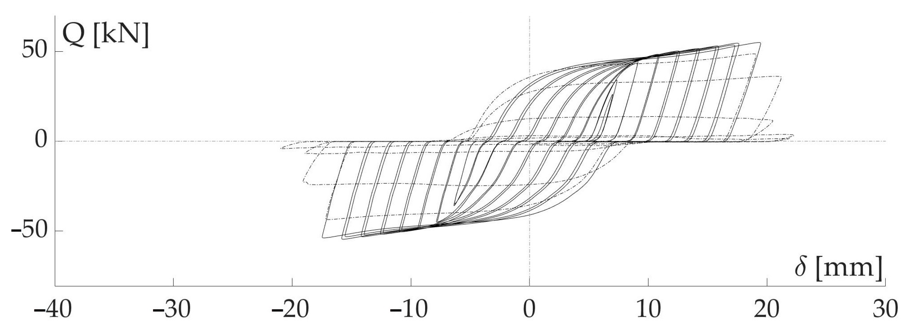
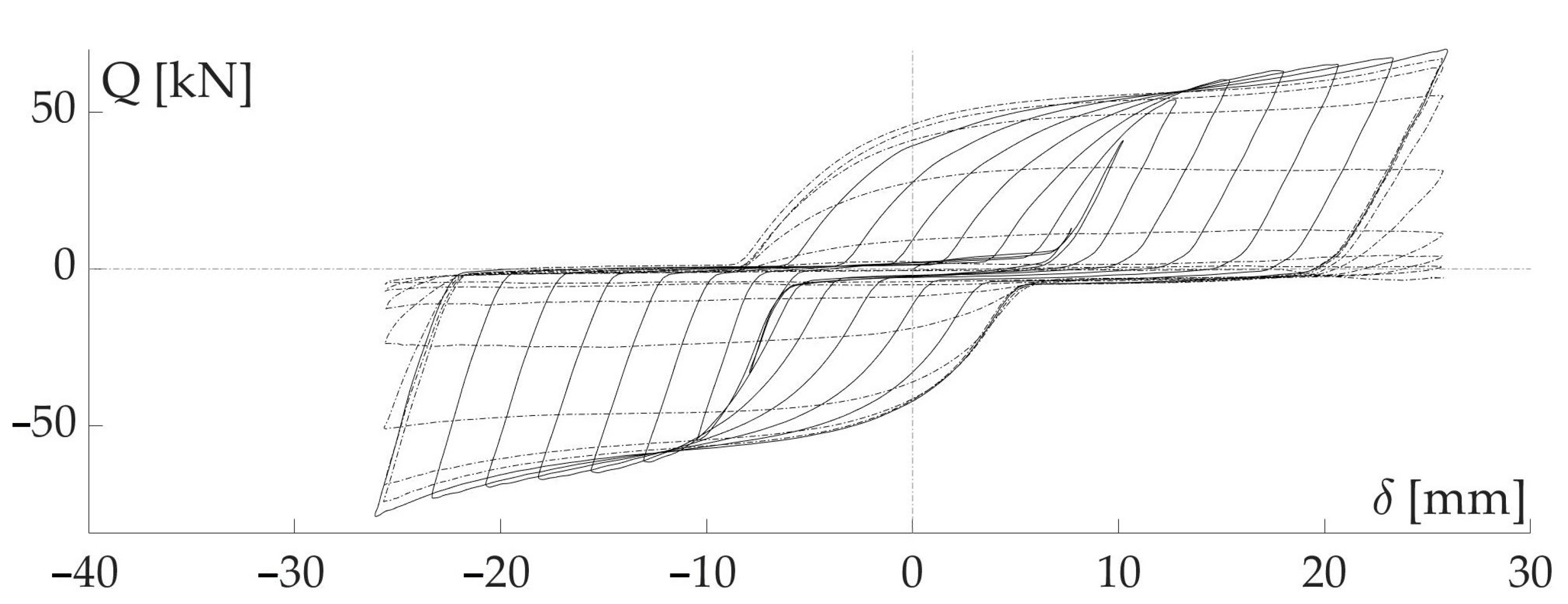
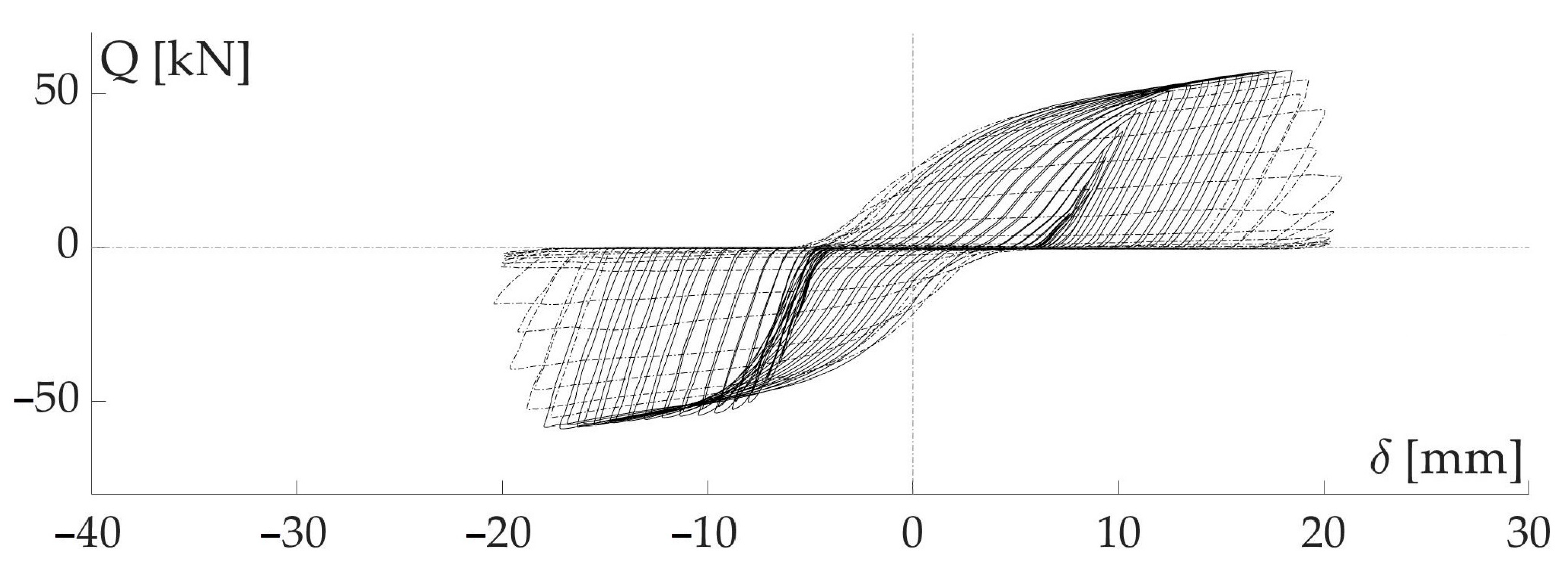
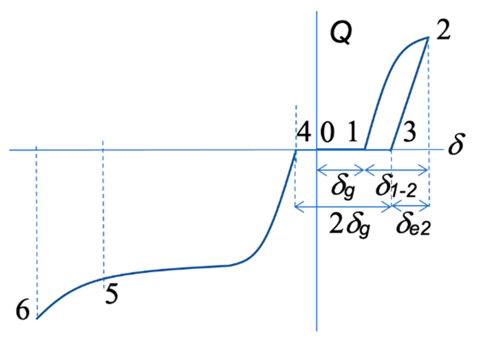
Figure 8, Figure 9 and Figure 10 show the load Q versus displacement loops obtained in the quasi-static tests. The two most noteworthy characteristics of these curves are: (i) the shifts of the loops along the X axis due to the presence of the gap, and (ii) the increment of plastic stiffness in the large deformation range (beyond about 20 mm in Figure 9). These features are shown in Figure 11 and described next. First, there is a free movement in which both gaps are opened, which delays the engagement of the damper producing the horizontal segment 0–1. Second, one of the gaps closes and the steel strips start to deform following the loading segment 1–2. Third, upon unloading, the sign of the displacement changes moves from point 2 to 3, and follows a line whose slope coincides with the initial elastic stiffness. Fourth, upon increasing the imposed displacements with the same sign (i.e., towards the negative horizontal axis), there is free movement until the other gap closes covering a distance along the X axis of (horizontal segment 3–4). Fifth, further increasing the imposed displacements with the same sign, the strip deforms, keeping approximately constant the restoring force Q until point 5. Sixth, when the deformations are very large, the restoring force Q starts to increase significantly (segment 5–6). The latter is caused by restriction on the movements of the ends of the strips in the direction perpendicular to the applied force Q (i.e., in the direction of the strip’s axis). In the specimens tested, the last (sixth) effect appears for axial deformations beyond approximately , which corresponds to an inter-story drift of about 1.5% in a conventional frame structure. The deformation associated with the onset of the overstrength (i.e., point 5 in Figure 11) depends on the level of restriction of the relative movements of the ends of the strips perpendicular to the axis of the MT-TTD, which can be tuned by controlling the stiffness of the lateral parts of the outer tube; that is, the inertia of the elements shown in Figure 5g with respect to the x–x′ axis passing through its centroid. Figure 8, Figure 9 and Figure 10 show with dot lines the force-displacement relationships after the peak strength is reached. It is worth noting that the degradation of strength after the assumed point of failure is gradual; this is due to the successive (i.e., not simultaneous) failure of the steel strips.
3.3. Dynamic Shake Table Tests
3.3.1. Experimental Set-Up
The performance of the MP-TTDs installed in a structure and subjected to realistic dynamic seismic loading was examined through shake table tests. Specimens MP-TTD-1 to MP-TTD-6 were installed as diagonal structural elements inside the column grid of a RC structure built at the Laboratory of Structural Dynamics of the University of Granada (Spain). The RC structure was a 2/5 scaled test specimen that represents a portion of a three-story prototype structure consisting of RC waffle-flat plates supported by RC columns. The structure was assumed to be located in the region of moderate-to-high seismicity of Granada (Spain) on soil type C (180 m/s < vs. < 360 m/s, where vs. is the shear wave velocity). The reference acceleration aR of the design earthquake (associated with a return period RP = 475 years) established by the 2012 Spanish seismic hazard map in rock is aR = 0.23 g (here g is the acceleration of gravity) and the soil amplification factor for soil type C is 1.34; therefore, the peak ground acceleration (PGA) of the “design earthquake” is 0.31 g (=0.23⋅1.34).
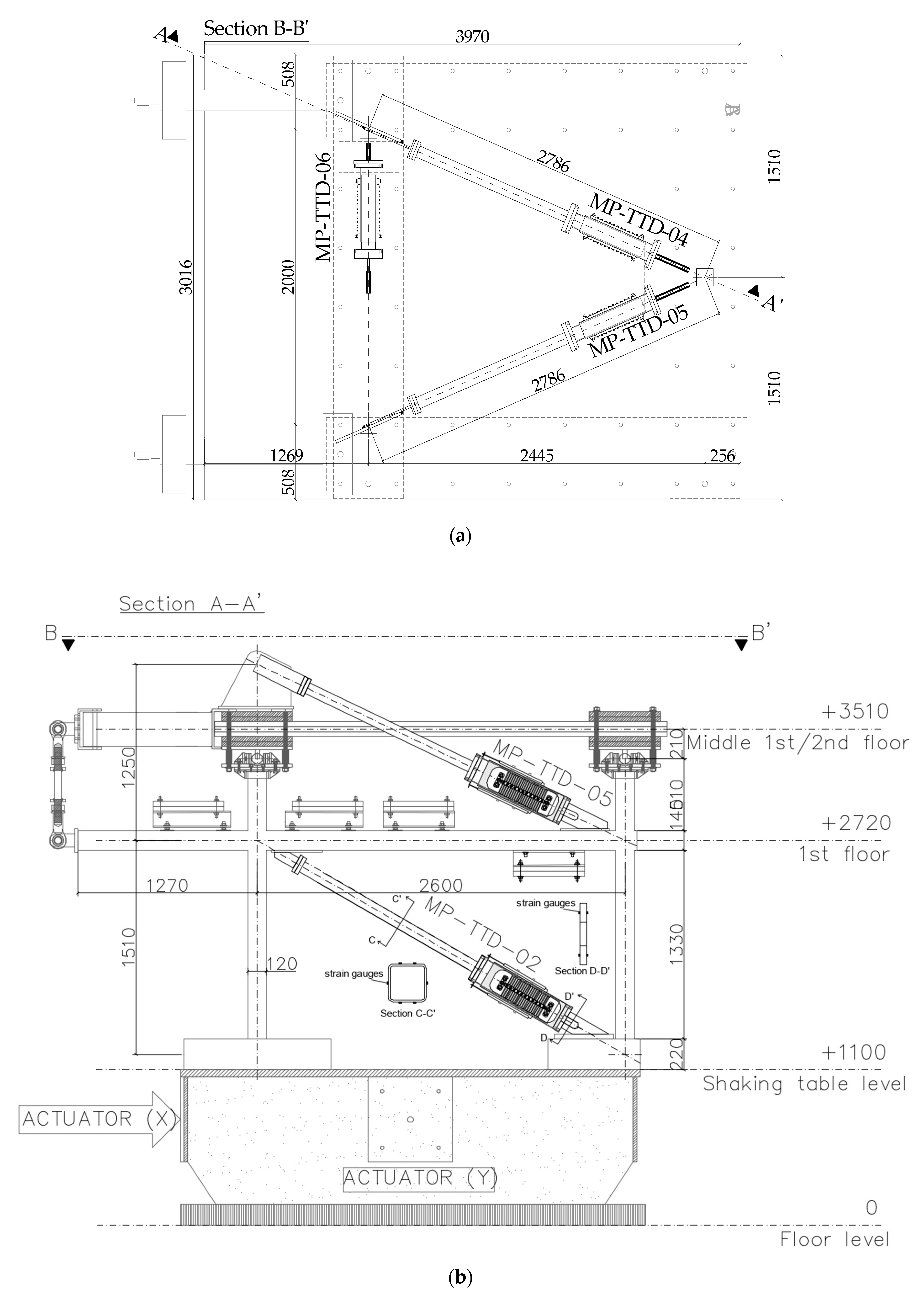
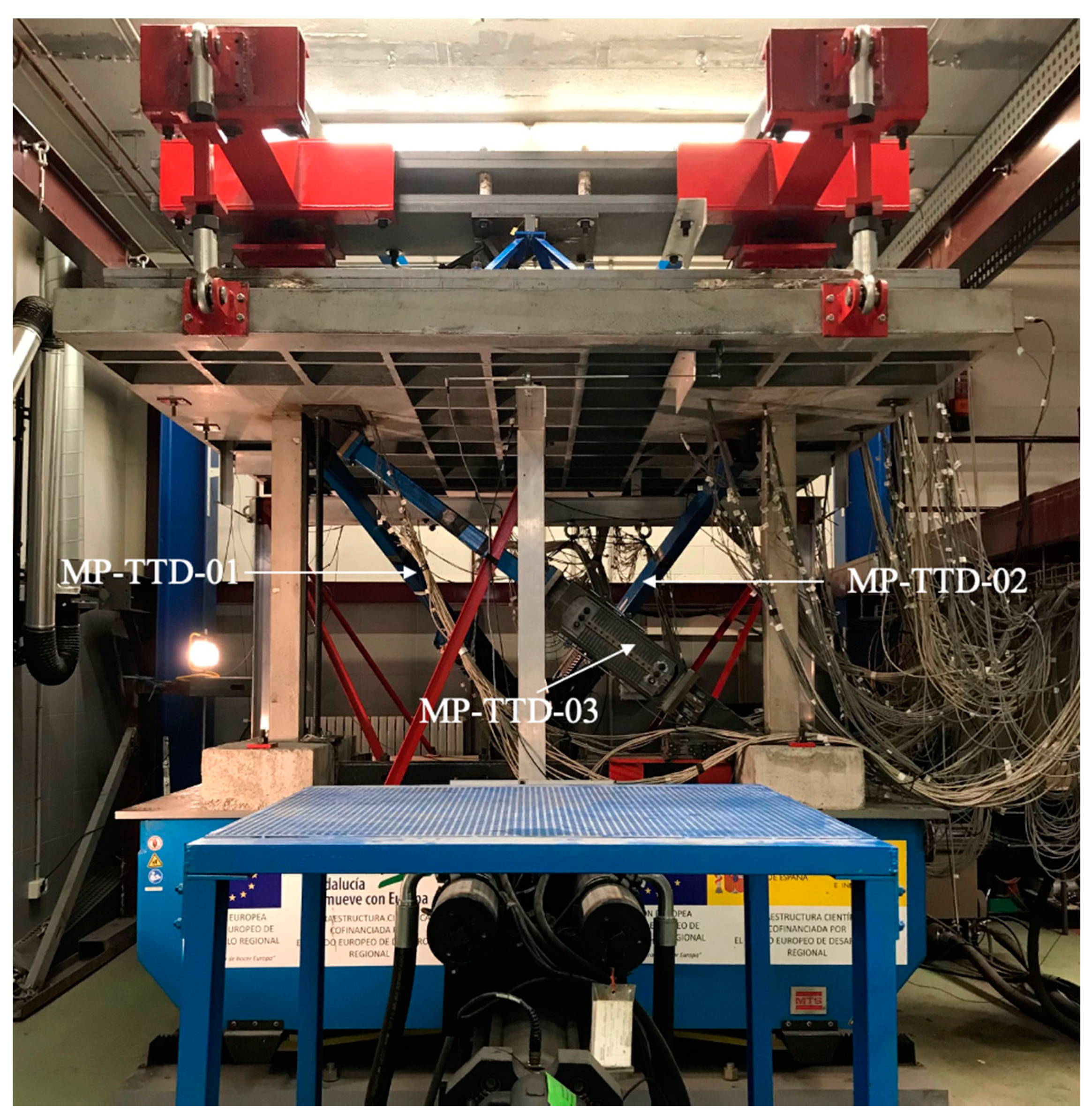
The RC test specimen comprises a waffle-flat plate supported on three rectangular columns, symmetrical along the X axis and irregular along the Y axis, as shown in Figure 12. Figure 13 offers a photograph of the RC structure with the MP-TTDs before the tests. Since this research is focused on the dampers, a detailed description of the RC structure is not pertinent. A detailed description of the RC structure can be found in [28]; in this reference a similar RC structure was tested with a different type of damper. In order to reproduce the inertial forces acting on the specimen during an earthquake, the total mass of the upper floors was replaced by steel plates pinned to the top columns. Each damper was instrumented with two displacement transducers (LVDTs) that measured the deformations along their axis. For each damper, the strains were measured at several points of two sections of the brace extenders; they are shown in Figure 12b for damper MP-TTD-02. One section (identified as section C-C′ in Figure 12b) was located at the middle of the upper brace extender and strains were measured at six points. The other section was at the lower brace extender (identified as section D-D’ in Figure 12b) and strains were measured at four points. The average value of the strains measured by the gauges located in the same section (C-C′ or D-D′) was used to estimate the axial force acting in the section. The axial forces estimated in section C-C′ and in section D-D′ were close, but the value in section C-C′ was judged more reliable and was used as an axial force acting on the damper. Since these brace extenders remained perfectly elastic during testing, the axial force in the damper was readily obtained by multiplying the strain measured by the gauges by Young’s modulus and the cross-section of the brace extender.
3.3.2. Dynamic Loadings and Force-Deformation Curves of the Dampers
The dynamic tests were performed with the bidirectional MTS 3 × 3 m2 shake table (MTS, Eden Prairie, MN, USA) of the Laboratory of Structures of the University of Granada (Spain). Prior to the seismic tests, the control system of the shake table was trained with white noise signals; the table peak acceleration during this training was approximately ±0.05 g. During this training, the forces developed on the MP-TTD were zero, since the maximum displacements measured along their axes (ranging roughly ±2 mm) did not exceed the gap ( = 5 mm). This confirmed the satisfactory response of the MP-TTD under low intensity dynamic excitations, such as those induced by wind.
Once the shake table was trained, the RC structure with the MP-TTDs was subjected to four bidirectional seismic tests of increasing intensity, referred to here as C100, C200, C300 and C400. In each test, the shake table reproduced simultaneously the NS and EW horizontal components of the ground motion recorded at Calitri during the Campano-Lucano earthquake, scaled in time by the factor λt = 0.63 (in order to satisfy similitude requirements), and respectively scaled in amplitude to 100%, 200%, 300%, and 400%. The resulting peak accelerations applied to the shake table were 0.16 g, 0.31 g, 0.47 g, and 0.62 g. These peak accelerations can be related with the seismic hazard levels established for Granada. Seismic test C100 is associated with a return period of RP = 93 years, representing a frequent earthquake. C200 is associated with PR = 475 years and represents the “design earthquake”. C300 and C400 are respectively associated with RP = 1357 and RP = 2687 years, and represent very rare earthquakes (“maximum credible earthquakes”). Figure 14 shows the history of accelerations applied to the shake table in each direction during test C100.
The following discussion is focused on dampers MP-TTD-1, MP-TTD-2, MP-TTD-3, and MP-TTD-4, since dampers MP-TTD-5 and MP-TTD-6 remained perfectly elastic in all simulations, as indicated at the beginning of this section.
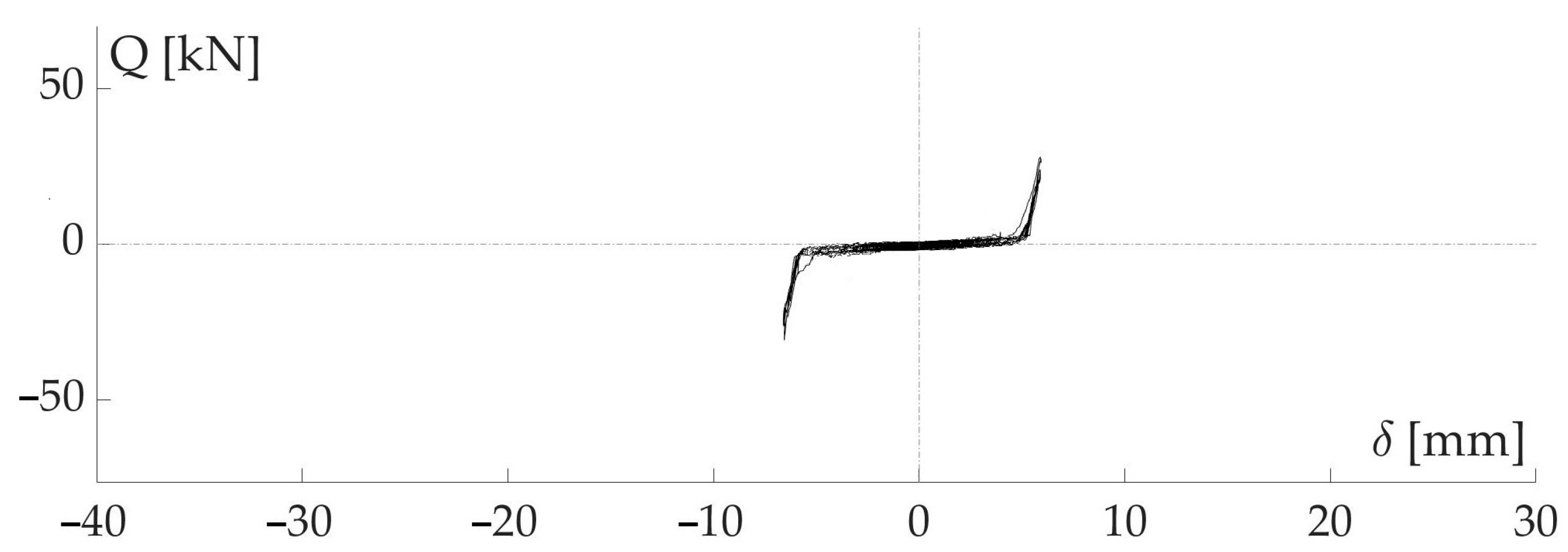
Seismic test C100 represents a frequent earthquake. During this test, the response of dampers MP-TTD-1, MP-TTD-2, MP-TTD-3, and MP-TTD-4 was basically elastic. The maximum displacements along the axis of the damper were up to about 7 mm, very close to the sum of the gap (5 mm) and the yield displacement (. Figure 15 shows, for illustrative purposes, the response of specimen MP-TTD-3; the other dampers behaved similarly. That is, under the “frequent earthquake”, the dampers enacted Phase II of their multi-phased behavior.
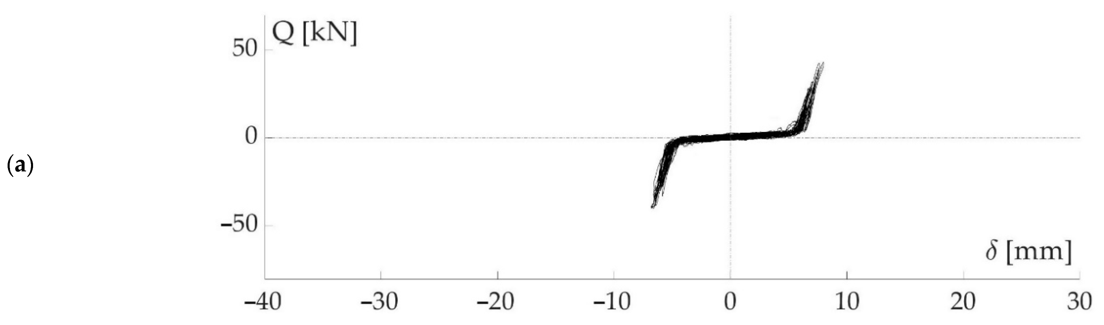
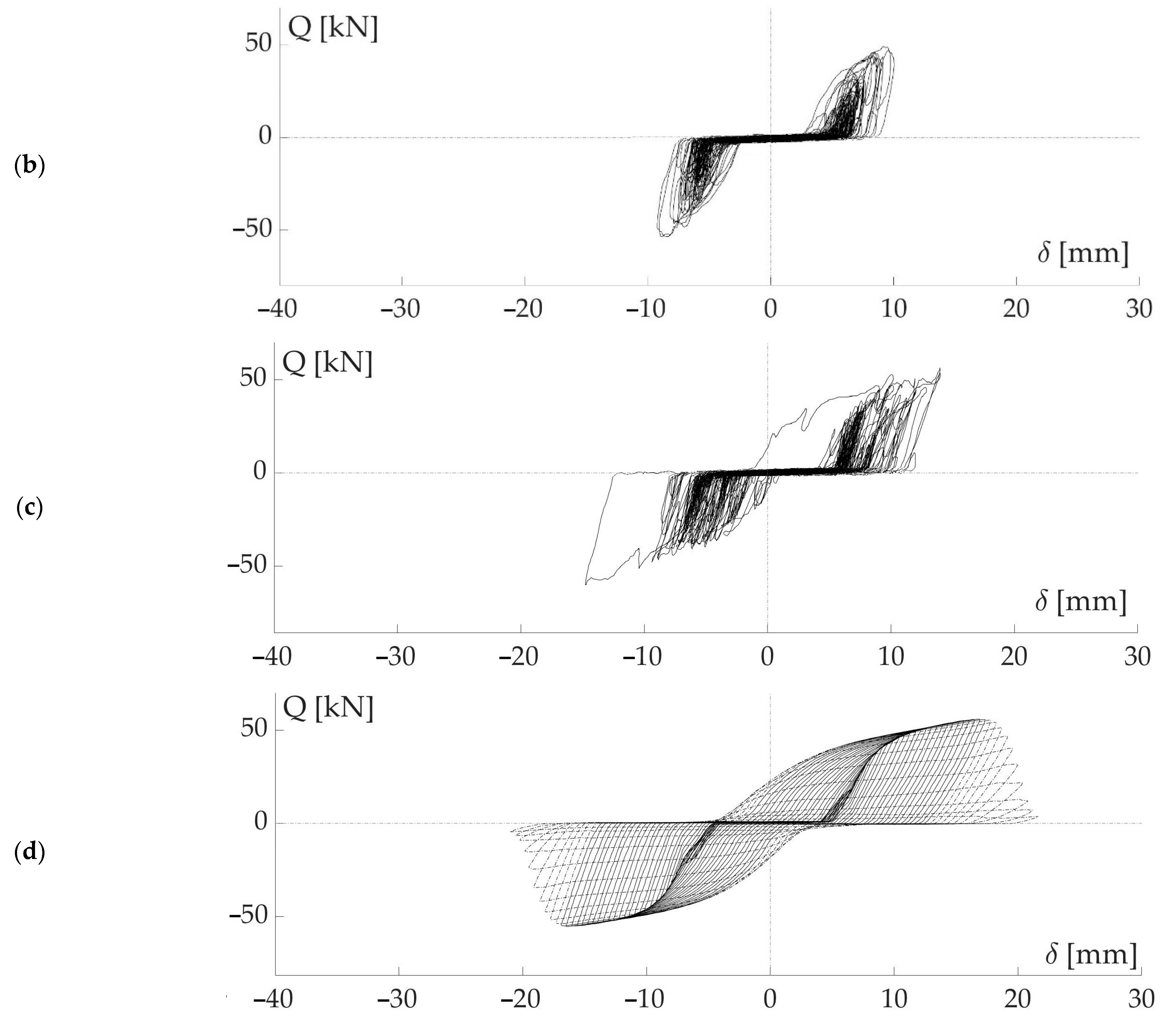
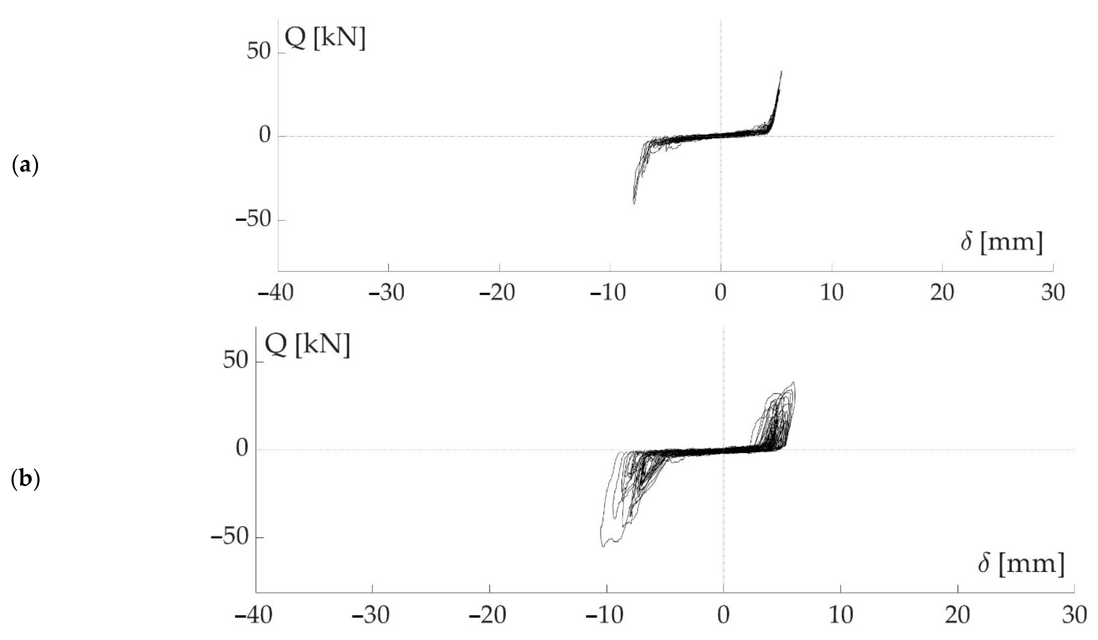
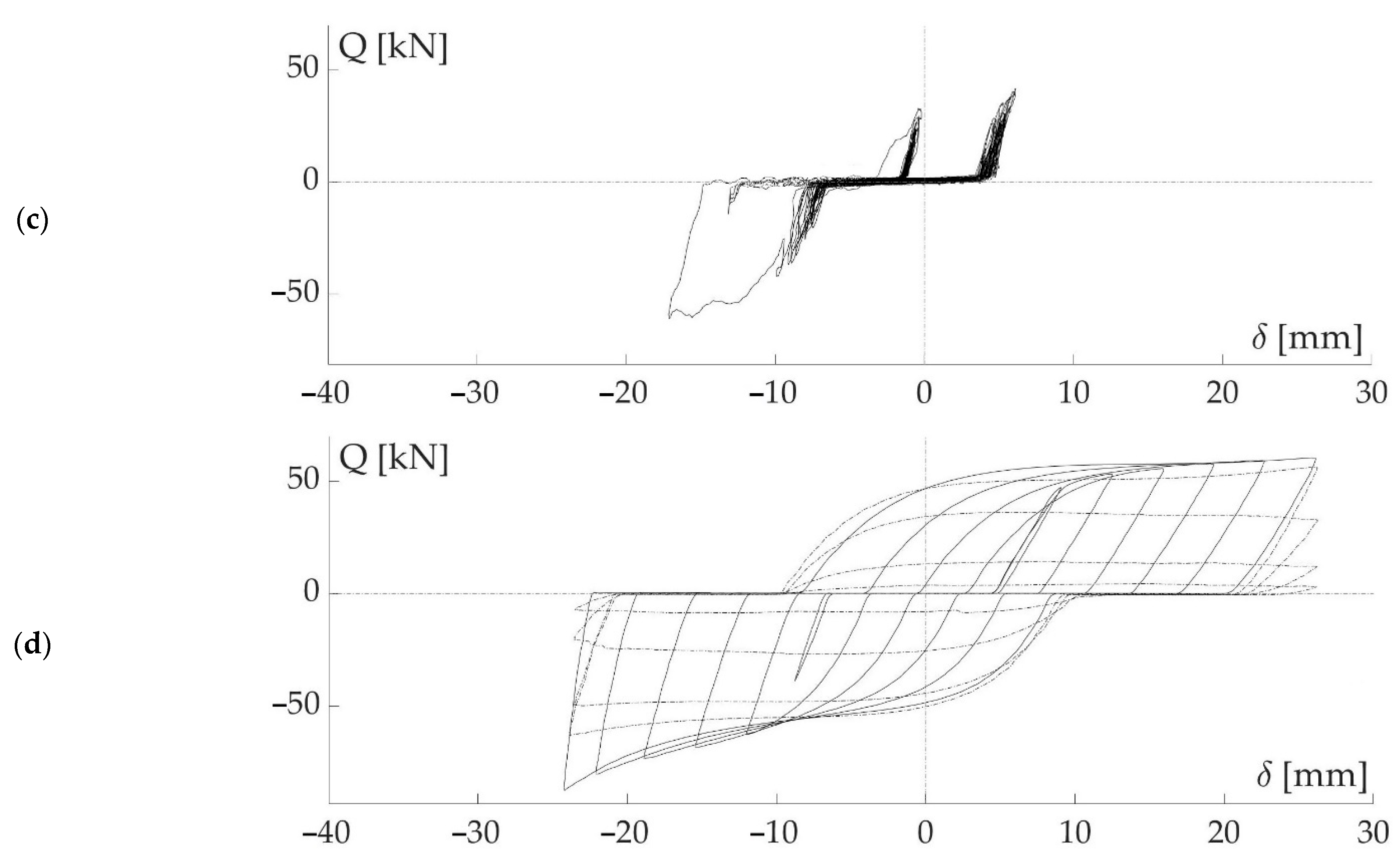
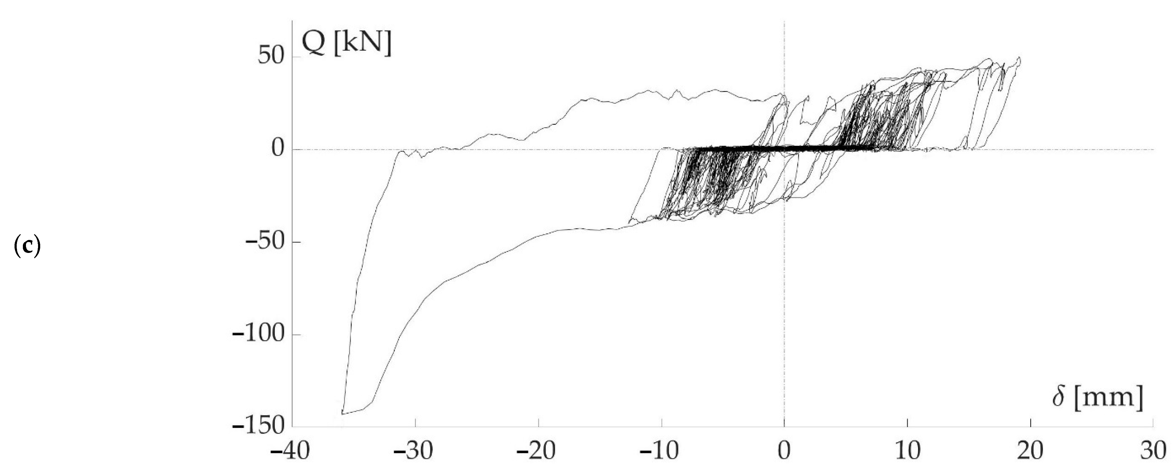
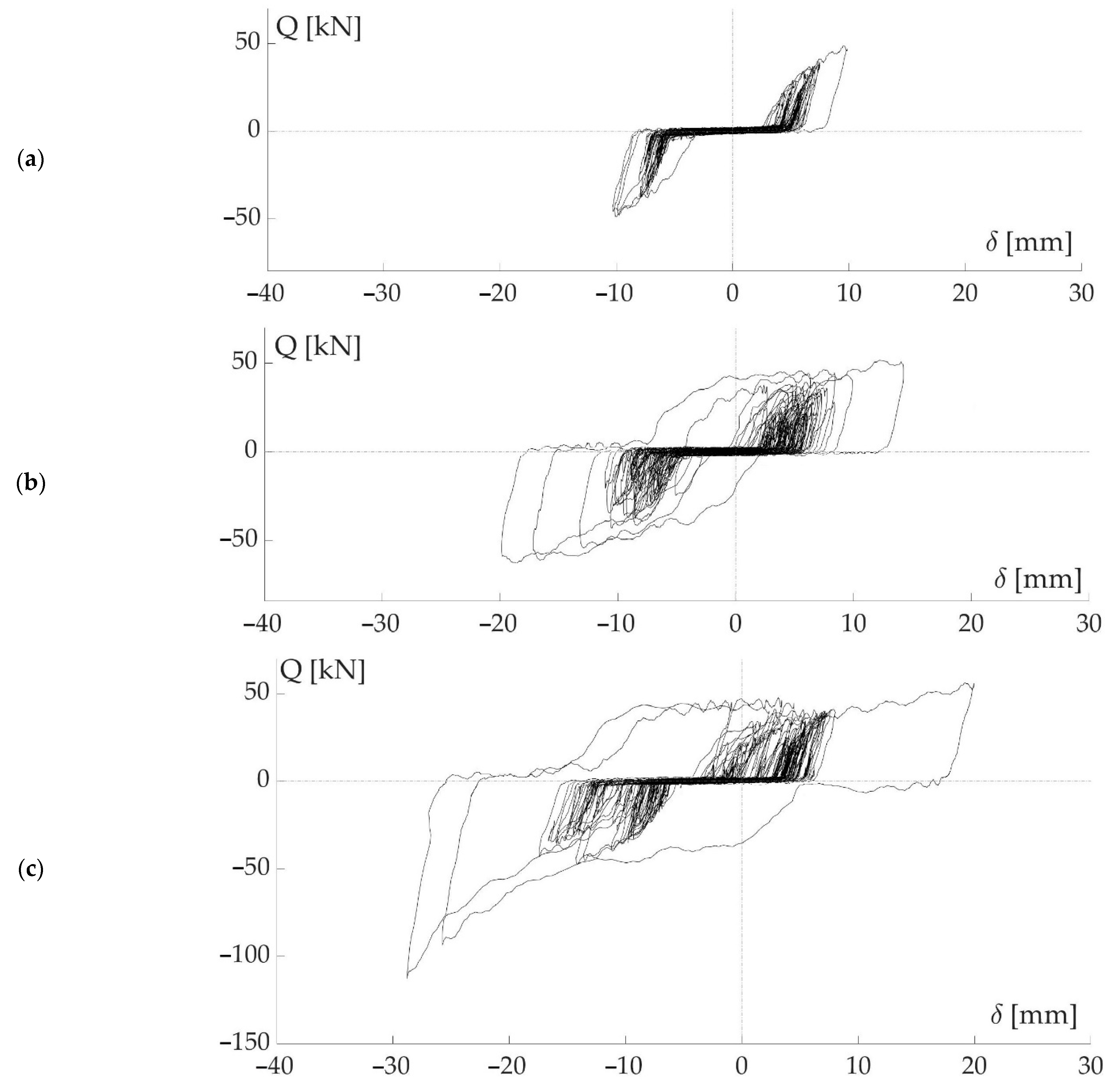
During seismic test C200, representing the “design earthquake”, the specimens MP-TTD-1 (Figure 16a) and MP-TTD-4 (Figure 17a) experienced some (minor) excursions in the plastic range, reaching maximum axial displacements of up to about 8 mm. In contrast, specimens MP-TTD-2 (Figure 18a) and MP-TTD-3 (Figure 19a) underwent significant plastic deformations, reaching maximum axial displacements up to 18 mm. This is far beyond the yield deformation (about 17 times , but no significant increase of strength or plastic stiffness is seen in the curve. This means that the dampers remained in Phase III under the “design earthquake”. The axial deformation corresponds to an inter-story drift of about 1.3% (=, where is the angle of the axis of the damper with the horizontal, and Hi = 1510 mm is the height of the first story of the RC structure). This inter-story drift is smaller than the upper bound value (1.5%) assigned by the Structural Engineers Association of California (SEAOC) in the well-known document Vision 2000 [29] to the performance level of “Life Safety”, meaning that the dampers protected the main structure satisfactorily and kept the RC frame within acceptable limits of lateral displacements. A careful inspection of the RC frame after test C200 served to confirm that it was basically undamaged (i.e., only minor hairline cracks in the concrete at the ends of the columns).
In turn, during seismic test C300, representing the “maximum credible earthquake”, dampers MP-TTD-1 (Figure 16b) and MP-TTD-4 (Figure 17b) underwent plastic deformations, though much smaller than those of MP-TTD-2 (Figure 18b) and MP-TTD-3 (Figure 19b). Particularly, the maximum axial deformation of damper MP-TTD-2 reached 30 mm (i.e., 28 times the yield deformation ), and the hysteretic curve presented a significant increase in strength and stiffness. This indicates that damper MP-TTD-2 entered Phase IV of its multi-phase behaviour. The maximum displacement of damper MP-TTD-3 was , and the curves do not reflect any significant increase of plastic stiffness; thus damper MP-TTD-3 did not enter Phase IV. In terms of maximum inter-story drift, the axial deformation corresponds to 2.3% (=). This value is close to the 2.5% assigned by SEAOC [29] to the performance level of “near collapse”. Inspection of the RC frame after test C300 showed only limited plastic deformations at column ends, but the RC structure kept its capacity to sustain the vertical loads, with no signs of being close to collapse.
Since the RC frame was not severely damaged and retained its capacity to sustain the vertical gravity loads, and since none of the dampers reached failure, it was decided that the seismic shakings should continue with the additional test, C400. It is worth recalling that C400 corresponds to a very rare earthquake, with higher intensity than the “maximum considered earthquake” prescribed by seismic codes for structures of normal importance (e.g., residential buildings). The return period of the earthquake simulated by test C400 (RP = 2687 years) is close to the value assigned by the European seismic code Eurocode 8 (2500 years) for verifying the “near collapse” limit of buildings pertaining to consequence class CC3a (i.e., buildings whose seismic resistance is of great importance in view of the consequences, e.g., schools, assembly halls, cultural institutions, etc.) During test C400, dampers MP-TTD-2 (Figure 18c) and MP-TTD-3 (Figure 19c) reached their ultimate energy dissipation capacity and failed. Both entered clearly in Phase IV of their multi-phase behaviour, as evidenced by the significant increases of strength and plastic stiffness. Before failure, dampers MP-TTD-2 and MP-TTD-3 were able to sustain extremely large axial deformations (39 mm MP-TTP-2 and 30 mm MP-TTD-3), up to 37 and 28 times the yield deformation, and develop very large forces of 145 kN (MP-TTD-2) and 110 kN (MP-TTD-3), which are about six times the nominal yield force Qy (=23.15 kN). These very large forces are attributed to the development of large axial forces along the axis of the steel strips when the damper is subjected to large deformations along its axis. The maximum deformation corresponds to an inter-story drift of 3% (=)—that is, above the value (2.5%) specified by SEAOC [29] as indicative of collapse. Inspection of the RC frame after test C400 revealed extensive plastic deformations at column ends, but the RC structure did not collapse. In sum, the overstrength and the associated increase of the plastic stiffness, together with the additional energy dissipation capacity provided by the dampers in Phase IV, prevented the RC structure from collapse under a ground motion of extreme severity with a PGA as large as 0.62 g. Dampers MP-TTD-1 (Figure 16c) and MP-TTD-4 (Figure 17c) also experienced large plastic deformations and maximum axial displacements up to , but they did not fail; they remained in Phase III. For this reason, in order to investigate their ultimate energy dissipation capacity, it was decided to subject dampers MP-TTD-1 and MP-TTD-4 to additional quasi-static cyclic deformations until failure, as explained below.
3.3.3. Additional Quasi-Static Tests Conducted on Dampers MP-TTD-1 and MP-TTD-4
Dampers MP-TTD-1 and MP-TTD-4 were subjected to additional quasi-static cyclic tests, using the experimental setup explained in Section 3.2. The histories of loading applied are indicated in Figure 20. They consisted of cycles of incremental amplitude, with ) equal to for damper MP-TTD-1 and to for damper MP-TTD-4, applied until the dampers failed. The additional hysteretic loops obtained are shown in Figure 16d and Figure 17d, respectively; it is worth noting that although the dampers were already severely damaged by previous dynamic tests, the hysteretic loops are very stable, showing no signs of strength or stiffness deterioration until the point where failure occurs. It is also noticeable that after the peak strength is reached, the strength degrades progressively, that is, it is not seen as a sudden drop of resistance.
4. Discussion
4.1. Decomposition into Skeleton and Bauschinger Parts
Previous research on metallic structural elements [30] has shown that the ultimate energy dissipation capacity is path-dependent, that is, it varies with the loading pattern applied. In the case of seismic loadings, the cyclic loading pattern that a future earthquake will impose upon a metallic damper cannot be foreseen, because the history of ground acceleration in itself is unpredictable. A convenient way to address this load-path dependency and characterize the energy dissipation capacity of the damper consists of decomposing the hysteretic loops into two parts: the so-called skeleton part and the Bauschinger part [31]. Let us consider the typical hysteresis Q-δ curve obtained for a damper until failure that is shown in Figure 21a. To simplify the explanation, and given that the presence of a gap, does not affect the decomposition, in the following explanation it is considered that .
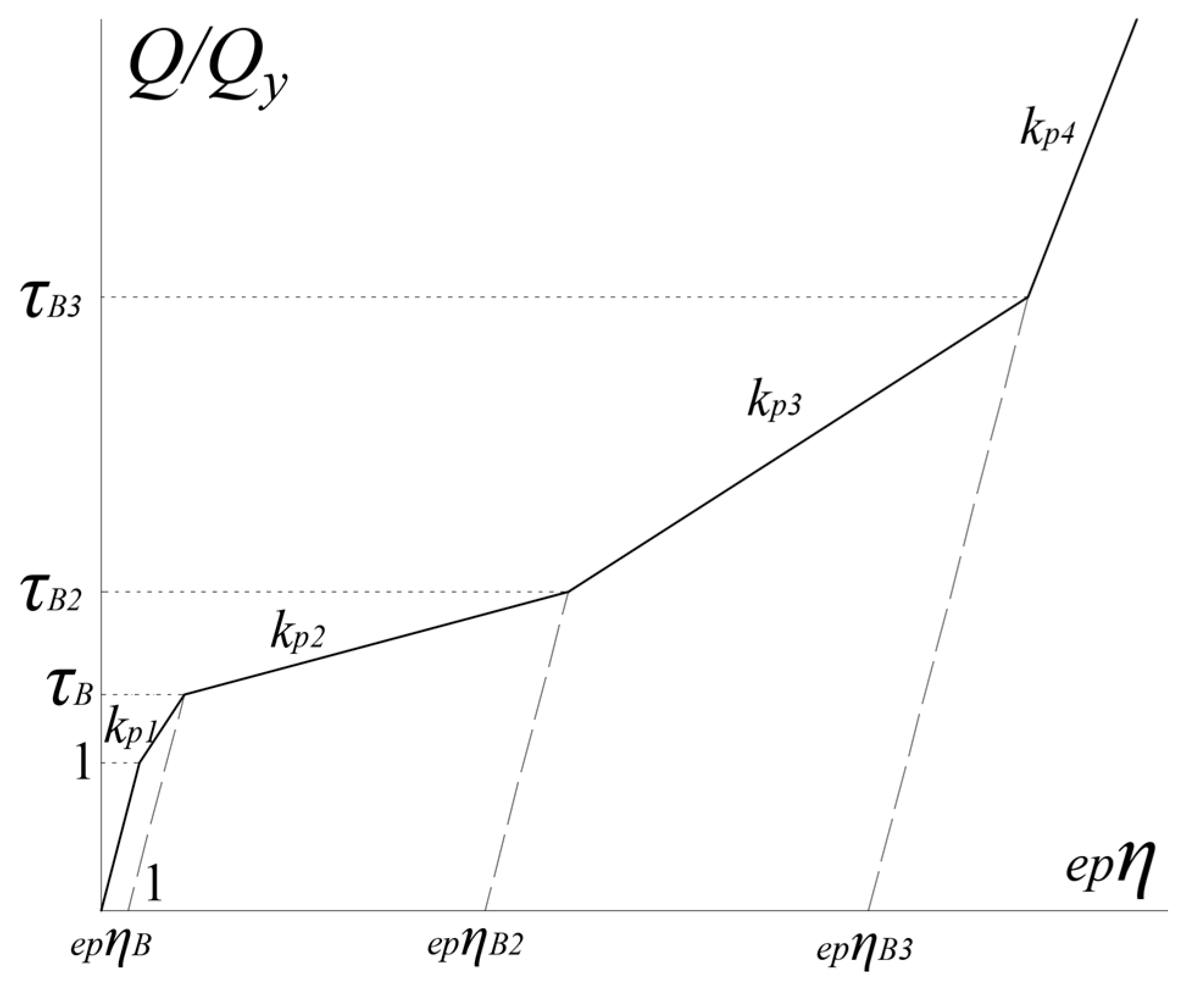
Within each domain of loading (positive or negative), the skeleton is defined through a sequential connection of the segments that exceed the maximum load Q attained by the metallic element in previous cycles of the same load domain. As depicted in Figure 21a, that would be the blue fragments 0–1, 5–6, 11–12, and 17–18 for positive loading, and 2–3, 8–9, and 14–15 for negative loading. Reassembling all the extracted skeleton parts successively in a continuous plot, the skeleton curve shown in Figure 21b is retrieved. Kato and Akiyama [31] showed that the shape of the skeleton curve is independent of the characteristics of the history of loading applied; but the end points, that is, the maximum accumulated deformations , do indeed depend on the loading history. Furthermore, these authors demonstrated experimentally that the shape of the skeleton part approximately coincides with the Q-δ relationship that would be obtained under monotonic loading. Given the independency of the shape of the skeleton part from the history of loading, the shape of the skeleton curves obtained for each damper were approximated in this study by a single pentalinear curve that is shown with dash and dot lines in Figure 21b. This pentalinear curve is characterized by Qy = 23.15 kN, QB = 33.89 kN, δy = 1.06 mm, Ke = Qy/δy = 21.83 kN/mm, Kp1 = 8.73 kN/mm; and Kp2 = 1.56 kN/mm, Kp3 = 3.64 kN/mm, Kp4 = 14.55, QB2 = 50.1 kN, QB3 = 96.4 kN. Referring to Figure 21b, the deformations , , corresponding to the end of the segments with stiffness Kp1, Kp2, Kp3, respectively, are , and . The values of Qy, QB and , can be predicted with Equations (1) and (2). For convenience, the approximated pentalinear skeleton curve can be expressed in nondimensional form in terms of the following parameters:
For the dampers tested in this study, their values are: kp1 = 2/5, kp2 = 1/14, kp3 = 1/6, kp4 = 2/3, , , .
The areas enveloped by the skeleton curves in each domain of loading (i.e., the shaded areas in Figure 21b) until will be denoted by SWu+ and SWu− and represent the energy dissipated by the damper on the skeleton part, in each domain of loading. Since depend on the history of loading, SWu+ and SWu− are different for each damper tested.
The Bauschinger part comprises the remaining segments of the Q-δ curve which, starting at Q = 0, seek the point corresponding to the maximum load attained in the preceding cycles for each loading domain. In Figure 21a that would be the green fragments 4–5, 10–11, and 16–17 for positive loading, and 7–8, and 13–14 for negative loading. Figure 21c shows all the Bauschinger parts extracted from Figure 21a and plotted correlatively. The sum of the areas enveloped by the Bauschinger parts in each domain of loading, BWu+ and BWu−, represents the fraction of the total plastic strain energy dissipated by the damper that is consumed on the Bauschinger part. The unloading branches in both the skeleton and Bauschinguer parts (i.e., segments 1–2, 6–7, 12–13, 18–19, 3–4, 9–10, and 15–16 in Figure 21b,c) have the initial elastic stiffness Ke.
4.2. Ultimate Energy Dissipation Capacity and Failure
Once the hysteresis Q-δ curve is decomposed into its skeleton and Bauschinger parts, the corresponding energies and the ultimate displacements for the positive and negative domains in the skeleton and Bauschinger parts can be expressed by the nondimensional parameters , and defined as:
The total energy dissipation in its nondimensional form for skeleton, Bauschinger and overall can be simply assessed as follows:
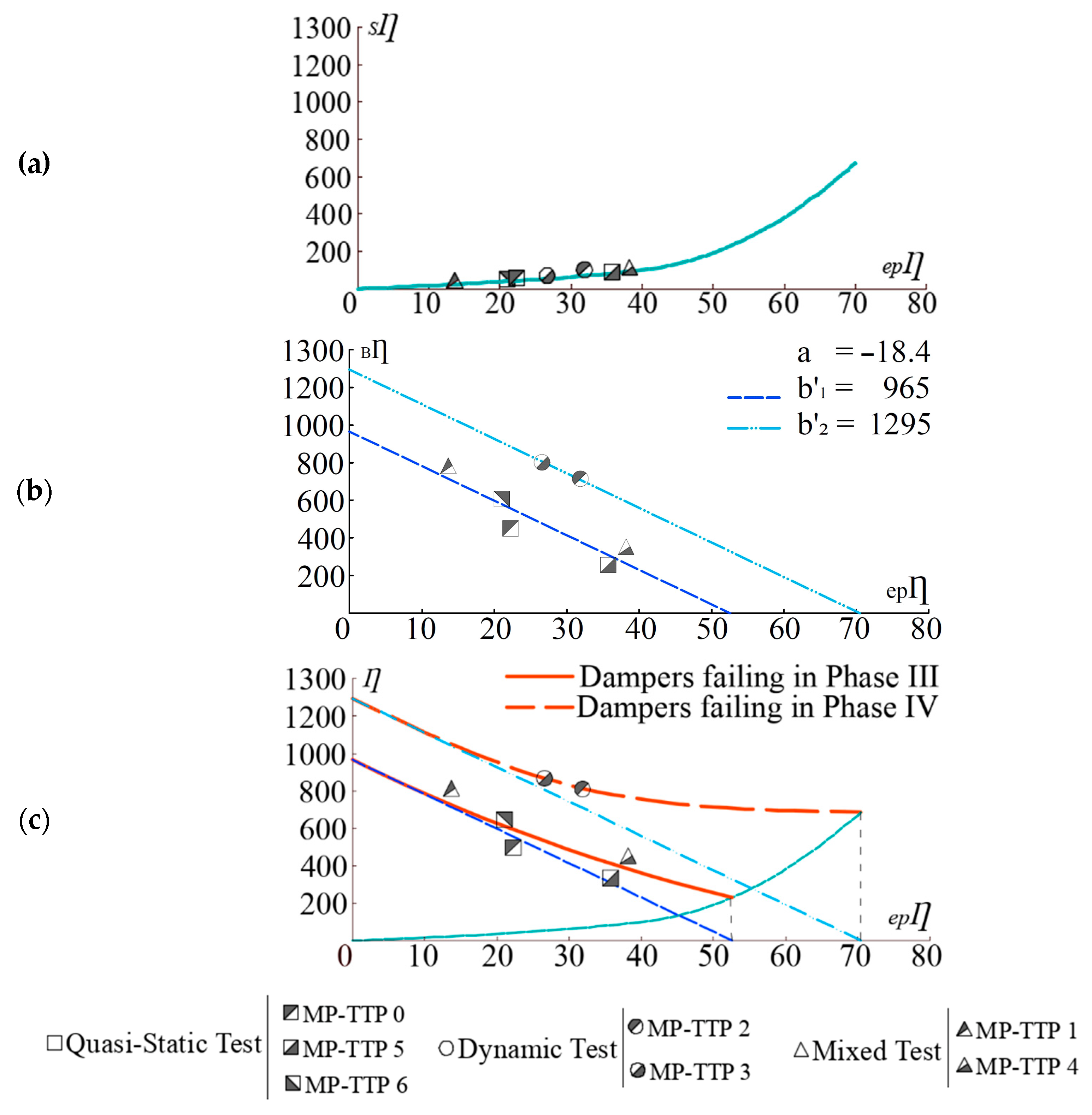
Following the procedure explained in Section 4.1, the Q-δ hysteresis loops obtained for each damper until failure were decomposed into the skeleton and Bauschinger parts. The values for the nondimensional ratios defined in Equations (3)–(5) were obtained and are summarized in Table 2 for the dampers that did not enter Phase IV, and in Table 3 for the dampers that entered Phase IV. Figure 22 plots the discrete values of , , and against . Both the dampers that did not enter Phase IV and those that entered Phase IV are represented together for comparison purposes.
Figure 22a shows the discrete values of against obtained from the tests. Since the relation between against depends only on the shape of the skeleton curve, it can be easily predicted from the pentalineal approximation of the skeleton curve adopted in Section 4.1 (see Appendix A). The curve predicted in this way is plotted in Figure 22a, with a solid bold line, and is given by:
For
For
For
For
Note that both the dampers not entering Phase IV and those entering Phase IV lie approximately on the same curve. This is because the shape of the skeleton curves is similar for all dampers, and is uniquely determined by the amount of deformation accumulated on the skeleton part .
Likewise, Figure 22b plots the discrete values of against . Two groups of points must be distinguished here. The first are the points corresponding to the dampers that did not enter Phase IV, and the second group those of the dampers that entered Phase IV. The points of the first group lie approximately on a line defined by:
With a = −18.4 and b’ = 965. On the other hand, the points of the second group lie on a line parallel to that of the first group of points, but displaced upward, vertically; the equation of the second line being determined by Equation (10) using a = −18.4 and b’ = 1295. This means that, for similar deformations accumulated on the skeleton part, the dampers that enter Phase IV dissipated about 35% more energy in the Bauschinger part that those that did not reach Phase IV.
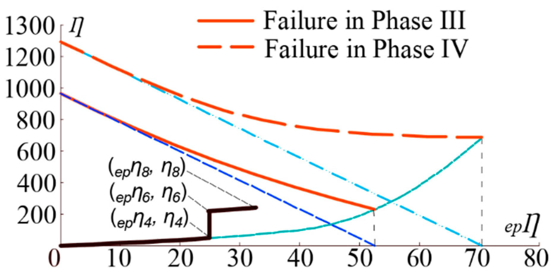
Finally, Figure 22c shows the total ultimate energy dissipation capacity. Since the curve corresponding to the Bauschinger part is different for the dampers that entered Phase IV and for those that did not, two curves (in red) are obtained for the normalized ultimate energy dissipation capacity. These curves can be used to predict the failure of the damper when subjected to arbitrarily applied loading (as would be induced by earthquakes), to be explained in the model proposed in the next section.
5. Model for Predicting the Hysteretic Curve under Arbitrary Cyclic Loading and Failure
The same rationale as explained in Section 4.1—to deconstruct the force displacement curve Q-δ obtained by subjecting a metallic damper to arbitrary cyclic loadings until failure—can be applied to construct (i.e., to predict) the hysteretic Q-δ loops developed by the damper if it is subjected to arbitrary cyclic loadings. It can be attained by means of a simple polygonal hysteretic model that requires characterization of the shape of the skeleton and Bauschinger parts. This is accomplished in the next subsections. Aside from its simplicity (easy implementation for example in subroutines for conducting non-linear time history analyses), the main advantages of the polygonal hysteretic model proposed next with respect to other well-known smooth hysteretic models based on the Bouc–Wen formulations are: (i) it can accurately reproduce the damper’s energy-consumption path along the skeleton and Bauschinger parts, and is therefore able to predict the failure of the damper; and (ii) it can accurately capture the significant increment of strength and stiffness in the range of large deformations.
5.1. Modelization of the Shape of the Skeleton Part
The shape of the skeleton part has been already been defined in Section 4.1; it is merely summarized here for convenience. The shape of the skeleton curve is characterized by Qy, QB, and calculated with Equations (1) and (2), and the nondimensional parameters kp1, kp2, kp3, kp4, , defined in Equation (3), whose values for the dampers investigated in this study are kp1 = 2/5, kp2 = 1/14, kp3 = 1/6, kp4 = 2/3, , , .
5.2. Modelization of the Shape of the Bauschinger Part
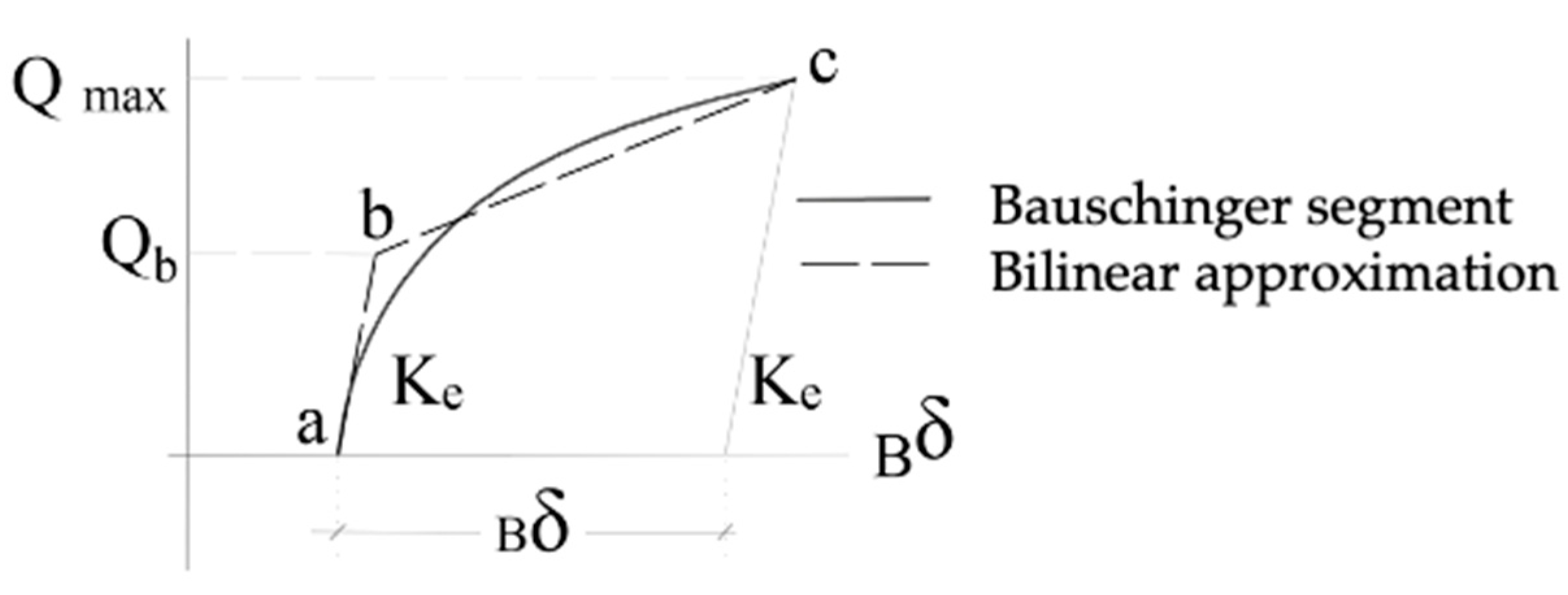
Each Bauschinger part, plotted in blue in Figure 21c, can be approximated by two lines as shown in Figure 23. The first segment starts at point “a”, whose ordinate is Q = 0, and ends at point “c”, whose ordinate is the maximum force Qmax attained by the damper in previous cycles in the same domain of loading. The slope of the first line is taken to be equal to the elastic stiffness Ke. Having defined the bilinear approximation, it is necessary to know the value of the Bauschinger deformation that defines point “c”, and the ordinate of the point “b” in Figure 23. To this end, the shape of the Bauschinger segments obtained in the tests were analyzed as follows. First, for a given Bauschinger segment whose deformation is , the amount of deformation accumulated on the skeleton part, , up to the start of this Bauschinger segment, was computed. For instance, given the Bauschinger segment 10–11 of Figure 21a (see Figure 21c), would be the sum of the deformation accumulated on the skeleton part until point 10, i.e., the deformation accumulated in the skeleton segments 0–1, 2–3, 5–6, and 8–9 in Figure 21a,b, hence . The pair of values () obtained in this way for the Bauschinger segments are plotted in Figure 24a. They are seen to lie approximately in a line that can be expressed by:
With . Secondly, for a given Bauschinger segment whose maximum force at the end point is Qmax, the value of was computed, making the area below the actual Bauschingher segment (bold line in Figure 23) and the area below the bilinear approximation (dash line in Figure 23) equal. The pair of values () calculated in this way for the Bauschinger segments obtained from the tests are plotted in Figure 24b. They lie approximately in a line given by the following expression, where :
5.3. Hysteretic Model for Predicting the Hysteretic Curves
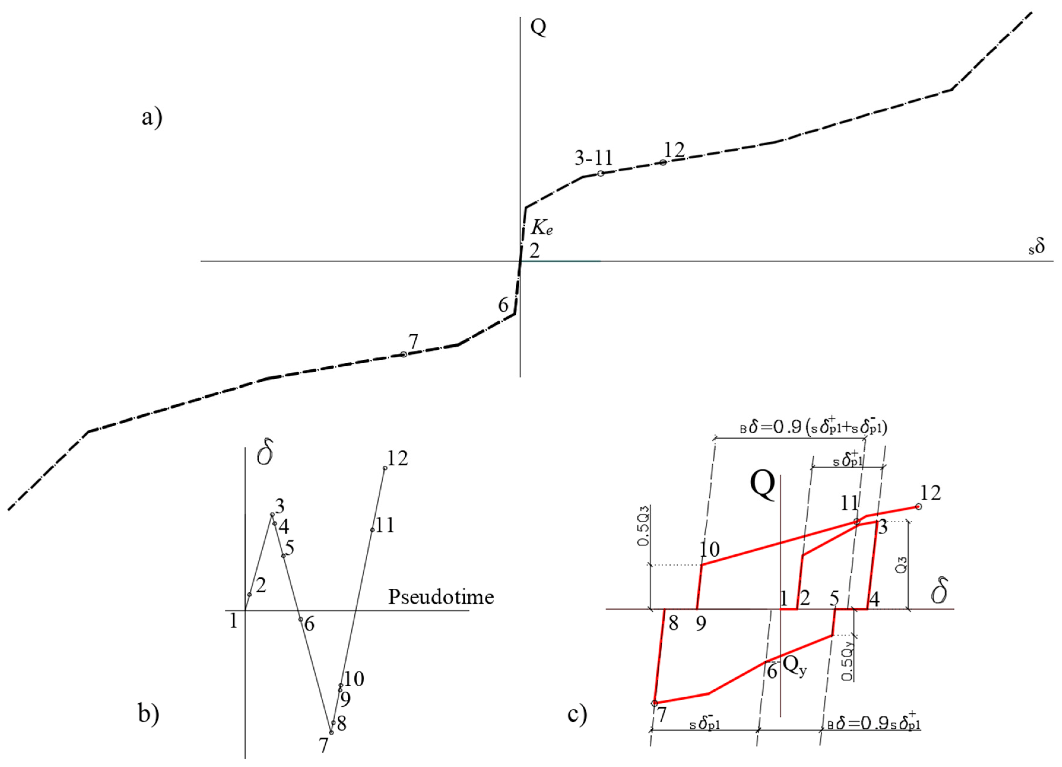
Once the shape of the skeleton and Bauschinger parts are defined, the construction of the force-displacement Q- hysteretic curve of the damper until failure is straightforward, being exemplified in Figure 25. Let us consider that the MP-TTD damper, whose skeleton curve is that shown in Figure 25a, has a gap , and is subjected to the history of forced displacements shown in Figure 25b. The Q-δ curve is shown in Figure 25c and it is constructed as follows. First, the damper is forced to move from point 1 to 3 in Figure 25b; from point 1 to point 2 the gap is opened and the force is zero. From point 2 to 3 the gap is closed, the damper is activated and it consumes the skeleton part following a Q-δ path that is equal to the segment 2–3 in Figure 25a. Second, the damper is forced to move from point 3 to point 7 in the loading history of Figure 25b. The segment 3–4 is an unloading branch with a stiffness equal to the elastic stiffness Ke. From points 4 to 5 the gaps are not closed and the damper displaces the amount 2 without opposing any force. Since before point 5 the damper has accumulated the plastic deformation on the skeleton part (i.e., from 2 to 3), the Q-δ curve starting at point 5 is a Bauschinger segment that ends at point 6, where Q = Qy, and it has the deformation amplitude , as prescribed by Equation (11). From point 6 onward, the damper again starts consuming the skeleton part (now in the negative loading domain) and the Q-δ curve coincides with the segment 6–7 in Figure 25a. Third, the damper is forced to move from point 7 to 12 in the loading history of Figure 25b. The initial segment 7–8 is an unloading branch of slope Ke. From 8 to 9 the damper deforms an amount 2 with a zero restoring force, since the gap is open. After point 9, the Q-δ curve is a Bauschinger segment ending at point 11 whose force is equal to the force at point 3, and the deformation amplitude is , as prescribed by Equation (11). The ordinate of point 10 is half the ordinate of point 3, as prescribed by Equation (12). From point 11 onward the damper starts consuming the skeleton part again, and the Q-δ curve coincides with segment 11–12 of Figure 25a.
The energy consumption path followed by the damper under the loading history of Figure 25b can be plotted in the plane of Figure 21c, which is redrawn in Figure 26 for convenience. The energy dissipated by the damper from point 1 to 4 in Figure 25c is the area below the Q-δ curve, W4, that can be expressed in nondimensional form by . Meanwhile, the deformation accumlated on the skeleton part up to point 4 in a nondimensional form is . The point of coordinates (, is shown in Figure 26. Since from point 1 to 4 all the energy has been consumed entirely by the skeleton part, the segment representing the load path 1–4 in the (, space follows the curve that represents the energy dissipated by the skeleton part. From point 4 to 6, the damper dissipates an increment of energy , where is the area of the Q-δ curve between points 4 and 6 in Figure 25c. Since between these points all the dissipated energy consumed only the Bauschinger part, then and the segment 4–6 in the (, space is a vertical line. The end point of coordinates (, is shown in Figure 26. From point 6 to 8, the damper dissipates an increment of energy , where is the area of the Q-δ curve between points 6 and 8 in Figure 25c. Between these points, all the dissipated energy consumed only the skeleton part with , then the segment 6–8 in the (, space is paralell to the curve that represents the energy dissipated by the skeleton part. The end point of coordinates (, is shown in Figure 26. Following this procedure, the energy consumption path in the (, space can be traced, and the damper will fail when the curve that represents the ultimate energy dissipation capacity of the damper is attained; yet if the damper does not enter Phase IV, the ultimate energy dissipation curve to be used is the solid red line of Figure 26; and if the damper enters Phase IV, the failure curve is the dash red line.
6. Conclusions
This paper investigated a new metallic damper intended for use in protecting structures subjected to earthquakes. The damper has a gap mechanism that prevents high cycle fatigue damage under wind loads. Seven identical specimens representing the damper were tested under quasi-static and dynamic loadings on a shake table until failure. The force-displacement curves were decomposed into the skeleton and Bauschinger parts to verify the shape of the hysteretic curves and the ultimate energy dissipation capacity of the damper. The following conclusions are reached:
1. The damper presents a very stable hysteretic response until failure, without any sign of strength or stiffness degradation.
2. The damper features a multi-phased behavior. In Phase I the damper is not activated because the gap is not closed. In Phase II the damper remains in the elastic range. In Phase III the damper dissipates energy through plastic deformations, keeping the restoring force approximately constant. In Phase IV the damper exhibits a significant increase in strength and stiffness, and keeps dissipating energy. The damper can be designed to remain in Phase I for wind loads, in Phase II for frequent earthquakes, in Phase III for the “design earthquake”, and in Phase IV for the “maximum credible earthquake”.
3. The ultimate energy dissipation capacity of the damper if it enters Phase IV is about 35% larger that if it remains in Phase III.
4. A simple polygonal hysteretic model is proposed to predict reasonably well the response of the damper under arbitrarily applied cyclic loads; it is able to capture the significant increase in strength and stiffness in the large deformation range.
5. Equations defining the ultimate energy dissipation capacity of the dampers are proposed, together with a criterion which, if applied in conjunction with the proposed hysteretic model, allows one to reliably and accurately predict the failure of the damper.
6. A reinforced concrete structure equipped with the new metallic dampers was tested on a shake table under realistic dynamic seismic loadings. During the preliminary low intensity white noise signals applied for training the shake table, the dampers did not become activated (i.e., they remained within Phase I). In the seismic tests representing a frequent earthquake, the damper remained elastic (i.e., within Phase II). Under the seismic test representing the “design earthquake”, the dampers experienced severe plastic deformations but did not exhibit any significant associated increase in strength/stiffness (i.e., they remained in Phase III), and they kept the main structure basically undamaged. Under the seismic tests that represented “maximum credible earthquakes”, the dampers exhibited a significant increase of strength and stiffness, entering Phase IV; this protected the main structure, limiting the damage and preventing collapse.
Author Contributions
Conceptualization, A.B.-C., and D.E.-M.; methodology, D.E.-M., J.A.-E. and H.P.-P.; software J.A.-E. and H.P.-P.; validation J.A.-E. and H.P.-P.; formal analysis J.A.-E.; investigation A.B.-C., D.E.-M., J.A.-E., H.P.-P.; resources A.B.-C.; data curation, J.A.-E., H.P.-P.; writing—original draft preparation D.E.-M.; writing—review and editing, A.B.-C.; supervision, A.B.-C.; project administration A.B.-C.; funding acquisition A.B.-C. All authors have read and agreed to the published version of the manuscript.
Funding
This research was funded by Spanish Ministry of Economy and Competitivity, research project reference MEC BIA2017 88814 R and received funds from the European Union (Fonds Européen de Dévelopment Régional).
Institutional Review Board Statement
Not applicable.
Informed Consent Statement
Not applicable.
Data Availability Statement
Data available on request due to restrictions e.g., privacy or ethical.
Conflicts of Interest
The authors declare no conflict of interest.
Appendix A
Figure A1 shows the approximated pentalineal skeleton curve in a given domain of loading (positive or negative) expressed in nondimensional form with the coefficients defined in Equations (3) and (6)–(9). Figure A2 shows with shaded areas a detail of the energy dissipated in the range (Figure A2a) and in the range (Figure A2b). For the range of deformation on the skeleton part a Figure similar to Figure A2b can be drawn replacing with and with . For the range of deformation on the skeleton part , a Figure similar to Figure A2b can be drawn replacing with and with .
The shaded area in Figure A2a can be expressed by:
Substituting x given by Equation (A2) in Equation (A3) gives:
Substituting x′ given by Equation (A6) in Equation (A7) gives:
Proceeding in the same way, for in the range is:
For
For
Noting that under cyclic loading the damper dissipates energy in the positive and in the negative domains of loading and assuming that , the total energy dissipated on the skeleton part is two times that expressed by Equations (A4), (A8)–(A10), and this gives the Equations (6)–(9) in Section 4.2.
Figure A1.
Normalized skeleton curve.

Figure A2.
Detail of the energy dissipated in the range: (a) and (b) .

References
- Skinner, R.I.; Kelly, J.M.; Heine, A.J. Hysteretic dampers for earthquake-resistant structures. Earthq. Eng. Struct. Dyn. 1974, 3, 287–296. [Google Scholar] [CrossRef]
- Soong, T.T.; Spencer, B.F., Jr. Supplemental energy dissipation: State-of-the-art and state-of-the-practice. Eng. Struct. 2002, 24, 243–259. [Google Scholar] [CrossRef]
- Constantinou, M.; Soong, T.; Dargush, G. Passive Energy Dissipation Systems for Structural Design and Retrofit; Monograph No. 1; MCEER: Buffalo, NY, USA, 1998. [Google Scholar]
- Symans, M.D.; Constantinou, M.C. Semi-active control systems for seismic protection of structures: A state-of-the-art review. Eng. Struct. 1999, 21, 469–487. [Google Scholar] [CrossRef]
- Housner, G.W.; Bergman, L.A.; Caughey, T.K.; Chassiakos, A.G. Structural control: Past, present, and future. J. Eng. Mech. 1997, 123, 897–971. [Google Scholar] [CrossRef]
- Chan, R.; Albermani, F. Experimental study of steel slit damper for passive energy dissipation. Eng. Struct. 2008, 30, 1058–1066. [Google Scholar] [CrossRef]
- Javanmardi, A.; Ibrahim, Z.; Ghaedi, K.; Ghadim, H.B.; Hanif, M.U. State-of-the-art review of metallic dampers: Testing, development and implementation. Arch. Comp. Meth. Eng. 2020, 27, 455–478. [Google Scholar] [CrossRef]
- Whittaker, A.S.; Bertero, V.V.; Thompson, C.L.; Alonso, L.J. Seismic testing of steel plate energy dissipation devices. Earthq. Spect. 1991, 7, 563–604. [Google Scholar] [CrossRef]
- Tsai, K.; Chen, H.; Hong, C.; Su, Y. Design of steel triangular plate energy absorbers for seismic-resistant construction. Earthq. Spect. 1993, 9, 505–528. [Google Scholar] [CrossRef]
- Kobori, T.; Miura, Y.; Fukuzawa, E.; Yamada, T.; Arita, T.; Takenaka, Y.; Miyagawa, N.; Tanaka, N.; Fukumoto, T. Development and application of hysteresis steel dampers. In Proceedings of the Tenth World Conference on Earthquake Engineering, Rotterdam, The Netherlands, 19–24 July 1992; pp. 2341–2346. [Google Scholar]
- Benavent-Climent, A.; Oh, S.; Akiyama, H. Ultimate energy absorption capacity of slit-type steel plates subjected to shear deformations. J. Struct. Constr. Eng. 1998, 63, 139–147. [Google Scholar] [CrossRef] [Green Version]
- Watanabe, A.; Hitomi, Y.; Saeki, E.; Wada, A.; Fujimoto, M. Properties of brace encased in buckling-restraining concrete and steel tube. In Proceedings of the Ninth World Conference on Earthquake Engineering, Tokyo-Kyoto, Japan, 2–9 August 1988; pp. 719–724. [Google Scholar]
- Oh, S.; Kim, Y.; Ryu, H. Seismic performance of steel structures with slit dampers. Eng. Struct. 2009, 31, 1997–2008. [Google Scholar] [CrossRef]
- Ghabraie, K.; Chan, R.; Huang, X.; Xie, Y.M. Shape optimization of metallic yielding devices for passive mitigation of seismic energy. Eng. Struct. 2010, 32, 2258–2267. [Google Scholar] [CrossRef] [Green Version]
- Zheng, J.; Li, A.; Guo, T. Analytical and experimental study on mild steel dampers with non-uniform vertical slits. Earthq. Eng. Eng. Vibr. 2015, 14, 111–123. [Google Scholar] [CrossRef]
- Lee, C.; Ju, Y.K.; Min, J.; Lho, S.; Kim, S. Non-uniform steel strip dampers subjected to cyclic loadings. Eng. Struct. 2015, 99, 192–204. [Google Scholar] [CrossRef]
- Amiri, H.A.; Najafabadi, E.P.; Estekanchi, H.E. Experimental and analytical study of block slit damper. J. Constr. Steel Res. 2018, 141, 167–178. [Google Scholar] [CrossRef]
- Shao, F.; Gu, T.; Jia, L.; Ge, H.; Taguchi, M. Experimental study on damage detectable brace-type shear fuses. Eng. Struct. 2020, 225, 111260. [Google Scholar] [CrossRef]
- Benavent-Climent, A. A brace-type seismic damper based on yielding the walls of hollow structural sections. Eng. Struct. 2010, 32, 1113–1122. [Google Scholar] [CrossRef]
- Lee, J.; Kim, J. Development of box-shaped steel slit dampers for seismic retrofit of building structures. Eng. Struct. 2017, 150, 934–946. [Google Scholar] [CrossRef]
- Marshall, J.D.; Charney, F.A. Seismic response of steel frame structures with hybrid passive control systems. Earthq. Eng. Struct. Dyn. 2012, 41, 715–733. [Google Scholar] [CrossRef]
- Lee, C.; Kim, J.; Kim, D.; Ryu, J.; Ju, Y.K. Numerical and experimental analysis of combined behavior of shear-type friction damper and non-uniform strip damper for multi-level seismic protection. Eng. Struct. 2016, 114, 75–92. [Google Scholar] [CrossRef]
- Hashizume, S.; Takewaki, I. Hysteretic-viscous hybrid damper system with stopper mechanism for tall buildings under earthquake ground motions of extremely large amplitude. Front. Built Environ. 2020, 6, 1–16. [Google Scholar] [CrossRef]
- Fang, Z.; Li, A.; Li, W.; Shen, S. Wind-induced fatigue analysis of high-rise steel structures using equivalent structural stress method. Appl. Sci. 2017, 7, 71. [Google Scholar] [CrossRef] [Green Version]
- Repetto, M.P.; Solari, G. Wind-induced fatigue collapse of real slender structures. Eng. Struct. 2010, 32, 3888–3898. [Google Scholar] [CrossRef]
- West, M.A.; Fisher, J.M.; Griffis, L.G. Serviceability Design Considerations for Steel Buildings; Design Guide 3; AISC: Chicago, IL, USA, 2003. [Google Scholar]
- Krawinkler, H. Guidelines for Cyclic Seismic Testing of Components of Steel Structures; ATC: Redwood City, CA, USA, 1992. [Google Scholar]
- Benavent-Climent, A.; Donaire-Avila, J.; Oliver-Saiz, E. Seismic performance and damage evaluation of a waffle-flat plate structure with hysteretic dampers through shake-table tests. Earthq. Eng. Struct. Dyn. 2018, 47, 1250–1269. [Google Scholar] [CrossRef]
- Structural Engineers Association of California (SEAOC) & Vision 2000 Committee. Vision 2000: Performance Based Seismic Engineering of Buildings; SEAOC & California Office of Emergency Services: Sacramento, CA, USA, 1995; Volume 1. [Google Scholar]
- Benavent-Climent, A. An energy-based damage model for seismic response of steel structures. Earthq. Eng. Struct. Dyn. 2007, 36, 1049–1064. [Google Scholar] [CrossRef]
- Kato, B.; Akiyama, H.; Yamanouchi, H. Predictable properties of structural steels subjected to incremental cyclic loading. In IABSE Symposium on Resistance and Ultimate Deformability of Structures Acted on by Well Defined Loads; International Association for Bridge and Structural Engineering: Lisbon, Portugal, 1973; pp. 119–124. [Google Scholar]
Figure 1.
Deformed shapes of slit-type steel plates with (a) simple or (b) double configuration, and (c) steel tubes with openings in the walls.
Figure 1.
Deformed shapes of slit-type steel plates with (a) simple or (b) double configuration, and (c) steel tubes with openings in the walls.

Figure 2.
Concept of the damper: (a) section A–A’; (b) elevation; (c) plan.

Figure 3.
Materialization of the metallic damper: (a) assembled damper; (b) outer tube; (c) inner tube; (d) photograph of the specimens used in the tests.
Figure 3.
Materialization of the metallic damper: (a) assembled damper; (b) outer tube; (c) inner tube; (d) photograph of the specimens used in the tests.

Figure 4.
Installation of the damper in a frame.

Figure 5.
MP-TTD damper specimen: (a) section A-A’; (b) elevation; (c) detail of the stoppers; (d) detail of a single steel strip; (e) cross-section; (f) cross-section; (g) detail of the part of the outer tube that restrains the movement of the ends of the strips along their axes. Units in mm.
Figure 5.
MP-TTD damper specimen: (a) section A-A’; (b) elevation; (c) detail of the stoppers; (d) detail of a single steel strip; (e) cross-section; (f) cross-section; (g) detail of the part of the outer tube that restrains the movement of the ends of the strips along their axes. Units in mm.

Figure 6.
Experimental set-up for quasi-static tests: (a) components, (b) photograph.

Figure 7.
Loading histories: (a) MP-TTD-0, (b) MP-TTD-5 and (c) MP-TTD-6.

Figure 8.
Force-displacement curves of damper MP-TTD-0.

Figure 9.
Force-displacement curves of damper MP-TTD-5.

Figure 10.
Force-displacement curves of damper MP-TTD-6.

Figure 11.
Main features of the force-displacement curves.

Figure 12.
Shake table test experimental set-up: (a) aerial plan view; (b) elevation. Units in mm.

Figure 13.
Photograph of the RC structure with the MP-TTDs before the tests.

Figure 14.
History of accelerations applied to the shake table in X (a) and Y (b) directions.

Figure 15.
Response of damper MP-TTD-3 during C100.

Figure 16.
Response of damper MP-TTD-1 during tests: (a) C200, (b) C300, (c) C400 and (d) quasi-static test.
Figure 16.
Response of damper MP-TTD-1 during tests: (a) C200, (b) C300, (c) C400 and (d) quasi-static test.


Figure 17.
Response of damper MP-TTD-4 during tests: (a) C200, (b) C300, (c) C400, and (d) quasi-static.
Figure 17.
Response of damper MP-TTD-4 during tests: (a) C200, (b) C300, (c) C400, and (d) quasi-static.


Figure 18.
Response of damper MP-TTD-2 during tests: (a) C200, (b) C300 and (c) C400.


Figure 19.
Response of damper MP-TTD-3 during tests: (a) C200, (b) C300 and (c) C400.

Figure 20.
Additional quasi-static loading histories: (a) MP-TTD-1 and (b) MP-TTD-4.

Figure 21.
Decomposition of Q-δ: (a) overall curve, (b) skeleton part and (c) Bauschinger part.

Figure 22.
Ultimate energy dissipation capacity: (a) skeleton part, (b) Bauschinger part, and (c) total energy dissipated.
Figure 22.
Ultimate energy dissipation capacity: (a) skeleton part, (b) Bauschinger part, and (c) total energy dissipated.

Figure 23.
Bilinear approximation of the Bauschinger segments.

Figure 24.
Parameters that characterize the shape of Bauschinger segments: (a) ; (b).

Figure 25.
Construction of the hysteretic curve: (a) skeleton curve, (b) load history and (c) hysteretic curve.
Figure 25.
Construction of the hysteretic curve: (a) skeleton curve, (b) load history and (c) hysteretic curve.

Figure 26.
Energy dissipation path and failure prediction.


Table 1.
Material mechanical properties.
| E (GPa) | σy (MPa) | σu (MPa) | εy (%) | εu (%) |
|---|---|---|---|---|
| 210 | 362 | 530 | 0.349 | 9.702 |
Table 2.
Ultimate energy dissipation capacity of the dampers that did not enter Phase IV.
| Specimen | Loading | Sδu+ | Sδu− | epη+ | epη− | Sη+ | Sη− | Bη+ | Bη− | Sη | Bη | η |
|---|---|---|---|---|---|---|---|---|---|---|---|---|
| MP-TTD 0 | Quasi-Static | 12.69 | 13.08 | 10.94 | 11.30 | 21.96 | 22.99 | 213.15 | 235.47 | 44.95 | 448.62 | 493.57 |
| MP-TTD 5 | Quasi-Static | 21.80 | 18.33 | 19.50 | 16.24 | 41.72 | 36.75 | 113.20 | 142.09 | 78.47 | 255.29 | 333.76 |
| MP-TTD 6 | Quasi-Static | 15.06 | 9.45 | 13.16 | 7.89 | 24.27 | 17.05 | 293.86 | 309.69 | 41.32 | 603.55 | 644.86 |
| MP-TTD 1 | Mixed | 6.24 | 10.43 | 4.87 | 8.81 | 10.78 | 19.09 | 376.73 | 389.42 | 29.87 | 766.15 | 796.02 |
| MP-TTD 4 | Mixed | 22.13 | 20.60 | 19.81 | 18.38 | 46.49 | 51.78 | 142.47 | 195.73 | 98.27 | 338.21 | 436.47 |
Table 3.
Ultimate energy dissipation capacity of the dampers that entered Phase IV.
| Specimen | Loading | Sδu+ | Sδu− | epη+ | epη− | Sη+ | Sη− | Bη+ | Bη− | Sη | Bη | η |
|---|---|---|---|---|---|---|---|---|---|---|---|---|
| MP-TTD 2 | Dynamic | 7.06 | 28.96 | 5.64 | 26.23 | 8,90 | 87.38 | 386.41 | 327.91 | 96.28 | 714.32 | 810.61 |
| MP-TTD 3 | Dynamic | 11.58 | 18.82 | 9.89 | 16.7 | 18.72 | 48.56 | 483.58 | 317.26 | 67.28 | 800.84 | 868.13 |
Publisher’s Note: MDPI stays neutral with regard to jurisdictional claims in published maps and institutional affiliations. |
© 2021 by the authors. Licensee MDPI, Basel, Switzerland. This article is an open access article distributed under the terms and conditions of the Creative Commons Attribution (CC BY) license (http://creativecommons.org/licenses/by/4.0/).
Share and Cite
MDPI and ACS Style
Benavent-Climent, A.; Escolano-Margarit, D.; Arcos-Espada, J.; Ponce-Parra, H. New Metallic Damper with Multiphase Behavior for Seismic Protection of Structures. Metals 2021, 11, 183. https://doi.org/10.3390/met11020183
AMA Style
Benavent-Climent A, Escolano-Margarit D, Arcos-Espada J, Ponce-Parra H. New Metallic Damper with Multiphase Behavior for Seismic Protection of Structures. Metals. 2021; 11(2):183. https://doi.org/10.3390/met11020183
Chicago/Turabian StyleBenavent-Climent, Amadeo, David Escolano-Margarit, Julio Arcos-Espada, and Hermes Ponce-Parra. 2021. "New Metallic Damper with Multiphase Behavior for Seismic Protection of Structures" Metals 11, no. 2: 183. https://doi.org/10.3390/met11020183
Note that from the first issue of 2016, this journal uses article numbers instead of page numbers. See further details here.