Analyzing Operational Efficiency in Real Estate Companies: An Application of GM (1,1) and DEA Malmquist Model

Abstract

Real estate management and its operation play a crucial role in supporting company operation. Going hand-in-hand with the rapid growth of companies, the real estate portfolio has expanded dramatically, attracting large numbers of domestic and foreign investors. This paper studied the top 12 real estate companies listed on Vietnam’s stock market to develop a method that combines the Grey methodology and the Data Envelopment Analysis (DEA) Malmquist model, intending to predict and evaluate their performances in two periods: 2015–2018 and 2019–2022. The proposed model considered three input factors, namely total assets, cost of sales, and cost of goods sold, and two output factors, namely total revenue and gross profit. Findings revealed that drastic efficiency changes in some companies should be observed at the beginning of the process, even if the technological efficiency in the period is stable. In the future period, most companies achieved relatively stable productivity. This study serves as a reference for policymakers and strategy makers by analyzing insights for the operational status of real estate businesses and providing an overview in the future toward sustainable development.

1. Introduction

Vietnam’s real estate market is gradually entering a period of financialization. The real estate industry’s contribution to GDP growth was 0.6% in 2010–2018. The relationship between investment capital and real estate value-added was 0.5%, while capital growth and value-added growth of this market reached 0.2%. This is because capital flows and financial resources were mobilized from different market segments such as industrial real estate, super-luxury apartments, the low-price housing market, the condominium market, project real estate, and the agricultural land market. The real estate market also plays an essential role in economic growth in Vietnam. From 2010 to 2018, affected by the world economy, the Vietnamese economy experienced many difficulties and challenges. The real estate market is facing a host of problems from credits and loans from the banking system. However, with the infrastructure built from 2005–2010, and at the end of the economic growth of 2014–2018, the real estate market had made positive contributions to Vietnam’s economic growth [1].

Currently, the real estate market is expanding and developing, which, in turn, promotes the development of infrastructures, increasing state budget revenues, expanding markets, and contributing to socio-economic stability. It is one of the factors in promoting an increase in investment capital. However, the real estate market is volatile. The influence of the world economy and the ever-changing socio-political environment has created many opportunities and challenges for the real estate market in Vietnam. Identifying the opportunities as well as the challenges to the market will help the real estate market find a solution to the growing problem in the future [2]. There are also other potential risk factors in the real estate market, such as the phenomenon of supply and demand deviation. There has been a sharp increase in secondary investors who tend to focus on a few large corporations investing in the luxury real estate and resort segments [3]. However, in many popular investment channels such as stocks, gold, and foreign currency, the return value of the investment fluctuates, requiring investors to be knowledgeable about the current trends or else the investor risks bankruptcy. In the meantime, real estate is a safe investment channel and has the highest profitability. Foreign investors invest in a company to reach new segments of the industry, such as industrial and resort real estates. Although investing in this industry is popular, there must be stricter regulations that make this industry more explicit and efficient [4].

Although the COVID-19 pandemic is spreading rapidly in many countries and causing severe damage to the global economy, Vietnam continues to effectively control the epidemic, ensuring economic activities are not interrupted. Even so, short-term economic growth is still significantly affected. In general, this is a difficult time for many domestic and foreign investors. However, for a group of individuals and businesses with effective market strategies and financial experiences, this is a great opportunity. Therefore, we hope that investors will seize this opportunity to make a reasonable investment choice [5].

In the future, Vietnam will have orientations and policy solutions to promote the development of the real estate market. For example, Vietnam has set a goal to reach the scale and economic level of an industrialized country by 2030, overcoming the middle-income trap. GDP per capita has reached at least USD 10,000 (the real price) or USD 18,000 (according to PPP price in 2011). The proportion of industry and services in GDP reached over 90% and contributed over 70% of employment. The shares of the private sector in GDP should be at least 80%. The human development index, according to the United Nations, is at least 0.7. Accordingly, the real estate market is expected to achieve sustainable development by 2030 with the following three pillars: (1) institutional improvement; (2) full development of components; (3) market growth to maturity level [1].

In brief, the identification and analysis of operational efficiency is a crucial task of managers in the market economy, which helps businesses to avoid losses in assets and capital and helps the sustainable growth of the economy. The information from this analysis will provide every audience inside and outside the business to make strategic decisions for each different purpose. In today’s economy, which is integrating and developing deeply with many unusual changes, it becomes more and more necessary to evaluate the performance of real estate businesses. In particular, in the sensitive business sectors such as the real estate market, the stock market, the information from the analysis and identification of financial signs is vital for businesses in general and listed real estate enterprises on Vietnam’s stock market in particular. In this paper, the researcher would like to introduce an overview of the current real estate industry so that entrepreneurs can identify opportunities and challenges to improve their business performance. The researcher will evaluate the business performance of the top 12 large real estate enterprises considered as Decision-Making Units (DMUs). These DMUs were screened by using Data Envelopment Analysis (DEA) method, the so-called DEA Malmquist model, and were listed on the stock market from 2015 to 2018 in Ho Chi Minh City, Vietnam, to help investors make the right decisions and ensure they would receive additional value from their investment. Grey theory, GM (1,1), is used to forecast the future data of DMUs and is applied as the input to the Malmquist model to assess the performance of these businesses in the future using the data from 2019–2022.

This paper includes five parts: (1) introduction, (2) literature review, (3) materials and methods, (4) empirical analysis and results, and (5) discussions and conclusions. First, the introduction part discusses the research problem and the objective of the paper. Then, the literature review describes and analyzes some of the previous related studies to show the motivation for this study. Following that, the materials and methods part provides the research process and a brief overview of methods applied in the paper. The fourth part presents a case study of real estate management in Vietnam and the model’s results. Finally, the discussions and conclusions part will summarize the highlights of this research and indicate some limitations for future studies.

2. Literature Review

In the past few decades, the DEA method has evolved into a powerful quantitative analysis and measurement tool for measuring and assessing performance. DEA has been successfully applied to various types of industries around the world. This paper discusses basic DEA models and their expansion. Since DEA in its present form was first introduced in 1978 by Charnes et al. [6], it was described as a mathematical programming model applied to experimental data that provided new ways to obtain practical estimates of relations such as the production of functions and/or productive capabilities surfaces. DEA became the basis for researchers of modern economies as some areas quickly realized that it was a great and easy-to-use method to model operational processes for performance evaluation. Drake and Hall [7] also employed DEA to analyze the technical and scale efficiency in Japanese banking; the results suggested that controlling for the exogenous impact of problem loans is important in Japanese banking. Bayyurt and Gokhan [8] used weighted DEA to determine the relative performance of Turkish and Chinese manufacturing companies. The results show that the average efficiency of Turkish manufacturing companies is less than that of Chinese manufacturing companies. Wang et al. [9] used the DEA method to help store affiliates find the right partner for the strategies. The results indicated that selecting a candidate for a strategic alliance can be an effective way for businesses to find a suitable partner.

According to the research of Färe et al. [10], the Malmquist Productivity Index (MPI) has two components; the first measures efficiency changes, and the second measures technological changes. Chang et al. [11] assessed the sustainability of corporations in 16 industries in China using the DEA Malmquist model and found that seven industries improved their sustainability performance and that the natural resources sector was more performative than the others. Wu et al.’s [12] study adopted DEA with the Malmquist Productivity Index (MPI) to assess the impact of intellectual capital on competitive advantage. The results showed that about one-third of the sampled companies had great efficiency in intellectual capital management, while others still have significant room to improve their intellectual capital management. The results of this study provided a valuable reference for future studies in an alternate context. In April 2013, Egilmez et al. [13] used the Malmquist model to evaluate the relative efficiency and productivity of 50 U.S. states in reducing the number of serious casualties. Single outputs, critical incidents, and five inputs are combined into a single road safety point and are used in the Malmquist mathematical model based on DEA approaches. As a result, reduced productivity (average of 0.2% of productivity) was considered in the United States in terms of reducing the number of serious accidents along with decreasing average efficiency by 2.1% and technology improvement by 1.8%. Productivity in reducing fatal accidents can only be due to technological growth because the effective growth in the negative direction is happening. It can be said that despite the downward trend in mortality rates, the efficiency of states in using social and economic resources for the goal of non-mortality remains ineffective. More effective policymaking to increase the use of safety belts and better use of safety costs to improve road conditions is considered a key area for high road safety agencies to focus on. Accelerated states are within the current study’s domain. Moreover, Vassdal and Sørensen [14] used MPI to measure the change in total factor productivity for production of Atlantic salmon in Norway from 2001 to 2008 and found that the total factor productivity change increased from 2001 to 2005 but thereafter regressed due to a regress in the technical change component of the MPI. This is an indication that the industry has reached a level of technological sophistication from which it is difficult to make substantial progress. The research also indicated that individual producers may still be able to improve efficiency by catching up relative to the best practice frontier.

The Grey system theory, founded by Deng [15] in 1982, is a new method for studying problems involving small patterns and poor information quality. This method checks for uncertain information in the system by establishing and seeking beneficial information from available sources. Therefore, many studies have applied the Grey theory in the past few years. For example, in 2010, Trivedi et al. [16] used the Grey theory and DEA models to predict storms for research areas with high accuracy. The 16 storm events for the Kothuwatari watershed of the Tilaiya dam catchment, Jharkhand, India, were collected in the years 1993–1997 and were used to develop and predict distinct hydrograph Grey models. The performance of the model has been assessed through qualitative and quantitative statistical indicators. The lower values of the different error indicators and the higher values of the correlation indicators confirm the ability of the storm flow prediction model with reasonable accuracy for the study area. In 2012, Wong et al. [17] researched the Comparisons of Fuzzy Time Series (CFTS) and Grey Model (GM). The results illustrate that the two forecasting models were appropriate for non-stationary time series. Among these models proposed, the GM residual modified model had a better predictive performance. The study also provides a beneficial reference for the hybrid Grey-based model in time series prediction. Besides, Wang et al. [18] also applied the Grey model (1,1) to predict future data. Based on the Mean Absolute Percentage Error (MAPE), the prediction was highly accurate. The results showed that in the first phase, the level of technical change was stable, and some major changes in technological changes of some companies needed to be observed. In the future phase, the performance of most companies increased steadily. This research provided an understanding of Thailand’s energy industry over the past few years and predicted its future performance.

In terms of real estate research, Jiang Yuan-yuan et al. [19] used DEA to analyze the efficiency of the real estate industry in Ningbo City. The inputs and outputs of an enterprise were used to reflect its production efficiency over a period; this process is called input–output analysis. The study was created to provide an accurate evaluation of the real estate market. The research results showed the development direction of the real estate industry, but it was not as accurate because the operational structure was left out. In 2014, Ge and Guo [20] used the DEA method to evaluate the performance and market efficiency of the top 100 real estate companies in 2012 listed on the Shanghai and Shenzhen stock markets. The researchers conducted DEA in two phases, separating the operational stage and the financial stage. The results showed that the participating companies with high performance accounted for about 75.9%, and among them, the companies with higher performance in the market only reached 14.8%. The reason is that the financial stage was not effective, and the market efficiency was low. Furthermore, Soetanto and Fun [21] used DEA to evaluate the performance of 23 real estate companies listed on the Indonesian stock market from 2009–2012. The results show that some companies are comparatively efficient each year. However, only one company always has a technical change with an index of 1. This proved that the company has a constant technical efficiency throughout 2019–2012. In general, most companies operating effectively showed an increase from 17.39% to 39.13%.

To the best of our knowledge, our paper is the first study on a two-stage model for the prediction and evaluation of real estate management in Vietnam by integrating GM (1,1) and DEA Malmquist model. In the proposed model, in the first stage, GM (1,1) is used to predict future data of the real estate market in 2019–2022 based on the historical data in 2015–2018. Then, in the second stage, the Malmquist model is used to evaluate the performance for the past and future periods of the top 12 DMUs in Vietnam. The managerial implications of this paper are to provide a beneficial guideline for the related decision-makers, policymakers, and managers in predicting and evaluating the performance of the real estate companies in Vietnam. This could also be used as a reference for other purposes.

3. Materials and Methods

3.1. Research Process

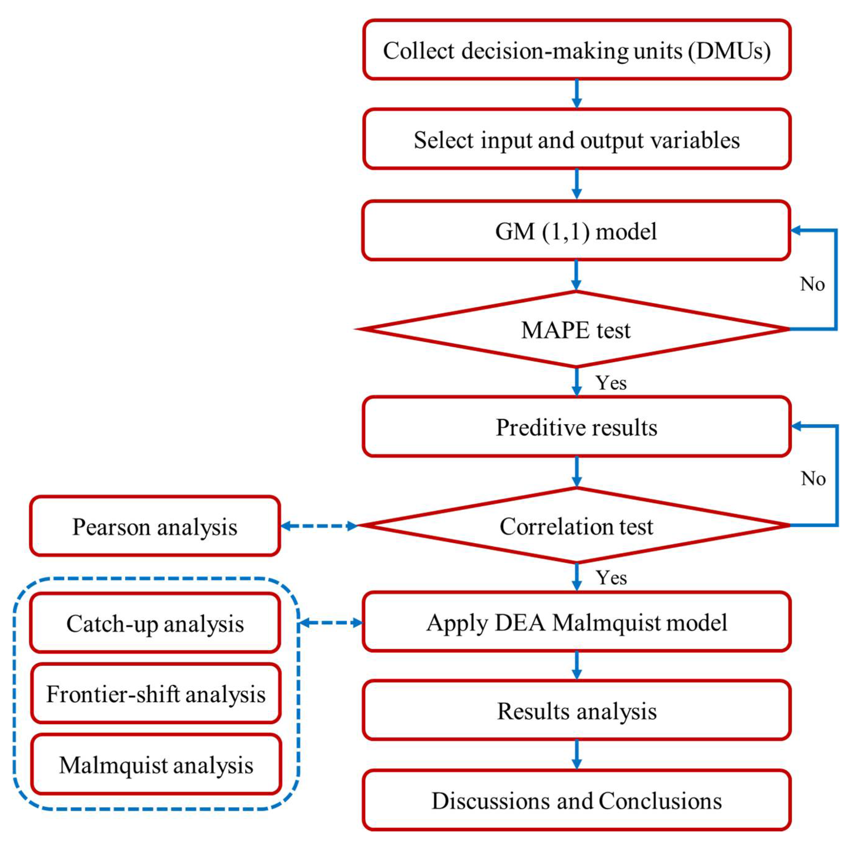
The research process (Figure 1) of the paper is described as follows. (Step 1) Choosing DMUs and collect relevant data: This step focuses on selecting the top DMUs in Vietnamese real estate companies and collecting their relevant information on the stock market from 2015 to 2018. (Step 2) Choosing input/output factors: Choosing inputs and outputs is an important step in applying the DEA model. This paper considered three inputs (total assets, cost of sales, cost of goods sold) and two outputs (total revenue, gross profit). (Step 3) Grey prediction: In this step, GM (1,1) is used to predict future data of inputs and outputs of DMUs. (Step 4) Checking forecasting accuracy: MAPE is used to check the predicted accuracy of GM (1,1). (Step 5) Pearson correlation test: The Pearson correlation method is used to check if the correlation coefficients between input and output factors are all positive correlation. (Step 6) DEA Malmquist model: The DEA method has different models each with different functions. MPI is used as the selected model to assess the changes in efficiency and performance in two periods: 2015–2018 and 2019–2022. (Step 7) Conclusion: The findings and summaries of the results from the proposed model are presented.

3.2. DMUs Selection

DEA is the most popular method in efficiency evaluation. It is a mathematical programming method for evaluating the relative efficiency of DMUs with multiple inputs and multiple outputs [22]. Therefore, selecting homogeneous DMUs with accurate data is also an essential step contributing to reflecting and evaluating the performance of DMUs. After researching companies in the field of real estate in Vietnam, the researcher selected the top 12 largest real estate companies and then collected and analyzed the data in four years (2015–2018). The list of all companies is shown in

Table 1. DMUs list.

DMUs	Name of Real Estate Companies	Symbol
REC-01	Long Hau Corporation	Long Hau
REC-02	De Tam Joint Stock Company	De Tam
REC-03	Ninh Van Bay Travel Real Estate	Ninh Van Bay
REC-04	PVC Petro Capital & Infrastructure Investment	PVC Petro
REC-05	Investment and Trading of Real Estate JSC	ITC
REC-06	Vincom Retail Joint Stock Company	Vincom
REC-07	LDG Investment Joint Stock Company	LDG
REC-08	Foreign Trade Development & Investment Corporation of HCMC	FDC
REC-09	Saigon Real Estate Joint Stock Company	Saigon
REC-10	Sonadezi Chau Duc Shareholding Company	Chau Duc
REC-11	Sonadezi Long Thanh	Long Thanh
REC-12	Tin Nghia Industrial Park Development Joint Stock Company	Tin Nghia

Source: https://vietstock.vn/ [23].

.

3.3. Inputs and Outputs Selection

This study aims to measure performance and implement investment decision-making strategies, and corporate data are collected from business reports on the stock market [23]. The accuracy of the data is very important because it can change the results significantly. Based on the impact of the financial indicators on the real estate industry and the summary of inputs and outputs used in previous relevant studies in

Table 2. The summary of inputs and outputs used in previous studies.

Authors	Input Factors	Output Factors	Methodologies
Yuan-yuan et al., 2010 [19]	Gross investments Land use Employees number	Gross revenue Sales amounts	CCR
Qi and Jia, 2010 [24]	Operation costs Employee salaries	Operation income Operation profit	Malmquist model
Peng Wong et al., 2012 [25]	Capital Assets value Operation costs Employees number	Revenue Profit	CCR SBM
Harun et al., 2012 [26]	Operating expenses Managing expenses Interest expenses	Total assets Total revenue Net assets value	CCR
Ge and Guo, 2014 [20]	Total assets Total operating costs	Operating income Net profit Earnings per share	CCR SBM Cost efficiency
Soetanto and Fun, 2014 [21]	Operating expense Fixed assets Land use	Net income	CCR
Wang et al., 2015 [27]	Total assets Prime operating cost Variable costs	Prime revenue Net profit	BCC
Chen and Li, 2017 [28]	Business cost Total assets Employees number	Business income Gross profit Return on equity	CCR BCC
Ahmed and Mohamad, 2017 [29]	Management fees Operating expenses Interest expenses	Total assets Net assets value Total revenue	Malmquist model
Atta Mills et al., 2020 [30]	Assets Capital Operating cost Employees number	Revenue Gross profit Return on equity	SBM Regression model
This paper	Total assets Cost of sales Cost of goods sold	Total revenue Gross profit	GM (1,1) Malmquist model

Notes: CCR: Charnes–Cooper–Rhodes, SBM: slack-based measure, BBC: Banker–Charnes–Cooper.

, this paper considered three input factors, including total assets, cost of sales, and cost of goods sold, and two output factors, namely total revenue and gross profit. The selected inputs and outputs are described as follows:

Input factors:

• Total assets (TA): the total assets owned by real estate companies.
• Cost of sales (CS): the cumulative total of all costs used to create a product or service that has been sold.
• Cost of goods sold (CGS): the direct cost of the product sold by real estate companies.

Output factors:

• Total revenue (TR): the total receipts that real estate business owners receive from the sale of goods or services.
• Gross profit (GP): the profit earned by the company after deducting expenses relating to the production and sale of its products, or expenses related to the provision of services by the company.

3.4. Grey Model

In recent years, the Grey prediction model has been very successful in many studies and has been used in many different fields. The GM (1,1) model is used most because this model provides a relatively high prediction rate while it only requires fewer periods of historical data (at least 4 periods) but can be applied in many different fields.

In this paper, because the number of data collected in the past is from only four years (2015–2018), the selection of this model to forecast future results is perfectly appropriate. Predicting future overview will be the basis to help investors make more accurate choices in the decision-making process. The procedures of setting up a GM (1,1) model are described as follows [15,31,32,33].

Let $x^{\left(0\right)}\left(k\right)$ is a set of the original string and $n$ is the total number of data, in Equation (1).

$$x^{\left(0\right)} =\left(x^{\left(0\right)}\left(1\right),x^{\left(0\right)}\left(2\right),\dots ,x^{\left(0\right)}\left(n\right)\right)$$

(1)

where $n$ denotes the number of observed data in a non-negative formula.

The one-time Accumulating Generation Operator (1-AGO) of the original string is specified in Equation (2). The purpose is to eliminate the bias and smooth the collected data.

$$x^{\left(1\right)}=\left(x^{\left(1\right)}\left(1\right),x^{\left(1\right)}\left(2\right), \dots ,x^{\left(1\right)}\left(n\right)\right)$$

(2)

where $\{\begin{array}{c}{x}^{\left(1\right)}\left(1\right)=x^{\left(0\right)}\left(1\right)\\ x^{\left(1\right)}\left(k\right)= {{\displaystyle \sum }}_{j=1}^k{x}^{\left(0\right)}\left(j\right)\end{array}, k = 2, 3, \dots , n.$

The generate mean $z^{\left(1\right)}$ of $x^{\left(1\right)}$ is defined, as can be seen in Equation (3).

$$z^{\left(1\right)}=\left(z^{\left(1\right)}\left(1\right),z^{\left(1\right)}\left(2\right),\dots ,z^{\left(1\right)}\left(n\right)\right)$$

(3)

where $z^{\left(1\right)}\left(k\right)$ denotes the mean value of adjacent data, as calculated in Equation (4).

$$z^{\left(1\right)}\left(k\right)= \frac{1}{2} \times \left(x^{\left(1\right)}\left(k\right)+x^{\left(1\right)}\left(\mathrm{k}-1\right)\right), k=2, 3,\dots ,n$$

(4)

From the one-time Accumulating Generation Operator (1-AGO) sequence $x^{\left(1\right)}$, the GM (1,1) model, which corresponds to the first-order differential term $x^1\left(k\right)$, can be built in Equation (5).

$$\frac{d{x}^{\left(1\right)}\left(k\right)}{dk}+a{x}^1\left(k\right)=b$$

(5)

where a and b are called the developing coefficient and Grey input in the model, respectively.

In practice, the value of a and b can be calculated as Equation (6), as follows.

$${\widehat{x}}^{\left(1\right)}\left(k+1\right)=\left(x^{\left(0\right)}\left(1\right)- \frac{b}{a}\right)e^{-ak}+ \frac{b}{a}$$

(6)

where ${\widehat{x}}^{\left(1\right)}\left(k+1\right)$ is the forecast value at period $\left(k+1\right)$.

To define the coefficient ${\left[a,b\right]}^T$, the Ordinary Least Squares method (OLS) is used, as can be seen in Equations (7)–(9).

$${\left[a,b\right]}^T={\left(A^{T}A\right)}^{-1}{A}^{T}Y$$

(7)

$$Y= \left[\begin{array}{c}{x}^{\left(0\right)}\left(2\right) \\ x^{\left(0\right)}\left(3\right)\\ \dots \dots \dots \\ \dots \dots \dots \\ x^{\left(0\right)}\left(n\right) \\ \end{array}\right]$$

(8)

$$A= \left[\begin{array}{cc}-\frac{z^{\left(1\right)}\left(2\right)}{2}& 1\\ -\frac{z^{\left(1\right)}\left(3\right)}{2}& 1\\ \dots \dots \dots & \dots \\ \dots \dots \dots & \dots \\ -\frac{z^{\left(1\right)}\left(n\right)}{2}& 1\end{array}\right]$$

(9)

where $Y$ denotes data series, $A$ denotes data matrix, and ${\left[a,b\right]}^T$ denotes parameter series.

Based on the values of ${\widehat{x}}^{\left(1\right)}\left(k+1\right)$ in Equation (6), let ${\widehat{x}}^{\left(0\right)}$ become the fitted and predicted series, as can be seen in Equation (10).

$${\widehat{x}}^{\left(0\right)}=\left({\widehat{x}}^{\left(0\right)}\left(1\right),{\widehat{x}}^{\left(0\right)}\left(2\right), \dots ,{\widehat{x}}^{\left(0\right)}\left(n\right)\right)$$

(10)

where ${\widehat{x}}^{\left(0\right)}\left(1\right)= x^{\left(0\right)}\left(1\right)$.

Applying the inverse accumulated generation operation. Equation (11) is obtained.

$${\widehat{x}}^{\left(0\right)}\left(k+1\right)=\left( x^{\left(0\right)}\left(1\right)- \frac{b}{a }\right)e^{-ak}\left(1-e^a\right)$$

(11)

MAPE is a measurement related to the predicted error. The MAPE is very useful to put forecasting performance into perspective, which is named ε [34] as in Equation (12).

$$\epsilon = \frac{1}{n} \sum \left(\frac{x^{\left(0\right)}\left(k\right)- {\widehat{x}}^{\left(0\right)}\left(k\right)}{x^{\left(0\right)}\left(k\right)}\right) \times 100\%$$

(12)

MAPE has an evaluation standard: a MAPE value < 10% is considered “excellent”, a MAPE value between 10–20% is considered “good”, a MAPE value between 20–50% is considered “qualified”, and a MAPE value > 50% is considered “unqualified” [35].

3.5. Data Envelopment Analysis (DEA)

To apply the DEA model, the relationship between inputs and outputs must be ensured to be isotropic, which means that if the number of inputs increases, the number of outputs cannot be decreased under the same conditions.

Pearson’s ($r_{xy}$) of two factors (x) and (y) is computed as follows [36].

$$r_{xy}= \frac{{{\displaystyle \sum }}_{i=1}^n\left(x_i-\overline{x}\right)\left(y_i-\overline{y}\right) }{\sqrt{{{\displaystyle \sum }}_{i=1}^n{\left(x_i-\overline{x}\right)}^2{{\displaystyle \sum }}_{i=1}^n{\left(y_i-\overline{y}\right)}^2}}$$

(13)

The correlation coefficients are explained in detail in

Table 3. Pearson correlation.

Correlation Coefficient	Degree
>0.8	Very high
0.6–0.8	High
0.4–0.6	Medium
0.2–0.4	Low
<0.2	Very low

Note: degrees of Pearson coefficient [36].

.

To assess productivity, it is important to identify the changes in the inputs and outputs of a company. The changes can be easily calculated in companies with only one input factor and one output factor. However, companies that have multiple inputs and outputs are more challenging to measure. When comparing the periods, the total factor productivity is used. The total factor productivity index is calculated using the two time periods symbolized by t and t + 1.

According to Färe et al. [37], the total factor productivity can be calculated using DEA. This process is called MPI. Unlike other main indexes of productivity evaluation, MPI does not need to have input and output prices. MPI can be calculated by multiplying technological changes (efficiency frontier shift) and technical efficiency (catching up the efficient frontier) [38].

MPI is calculated as the production of technical change and technological change, i.e., MPI = (catch-up) × (frontier-shift). Let the $DM{U}_i$ at the time period of 1 be $\left(x_0^1,y_0^1\right)$ and at the time period 2 be $\left(x_0^2,y_0^2\right)$. The efficiency score of the $DM{U}_i$ ${\left(x_0^1,y_0^1\right)}^{t1}$ is measured by the technological frontier t₂: $d^{t2}({(x_0, y_0)}^{t1})$ (t₁ = 1, 2 and t₂ = 1, 2).

Catch-up efficiency (C) can be defined as Equation (14).

$$C=\frac{ d^2({\left(x_0,y_0\right)}^2)}{d^1({\left(x_0,y_0\right)}^1)}$$

(14)

Frontier-shift efficiency (F) can be defined as Equation (15).

$$F= {\left[\frac{d^1({\left(x_0,y_0\right)}^1)}{d^2({\left(x_0,y_0\right)}^1)}\times \frac{d^1({\left(x_0,y_0\right)}^2)}{d^2({\left(x_0,y_0\right)}^2}\right]}^{\frac{1}{2}}$$

(15)

The ratio of technical efficiency in period t to t + 1 is called the catch-up effect, while the frontier-shift effect is based on the technological efficiency in period t to t + 1.

After calculating C and F, the following formula, Equation (16), was used to calculate the MPI.

$$\mathrm{MPI}= {\left[\frac{d^1({\left(x_0,y_0\right)}^2)}{d^1({\left(x_0,y_0\right)}^1)}\times \frac{d^2({\left(x_0,y_0\right)}^2)}{d^2({\left(x_0,y_0\right)}^1)}\right]}^{\frac{1}{2}}$$

(16)

The results of the Malmquist model are divided into three cases [39]: (1) If MPI > 1, represents a productivity improvement. (2) If MPI = 1, represents constant productivity. (3) If MPI is < 1, represents a decrease in productivity.

4. Empirical Analysis and Results

4.1. Results of the Grey Model

The historical data of the years 2015–2018 are presented in

Table A1. The historical data of the year 2015, (unit: million USD).

DMUs	(I) Total Assets	(I) Cost of Sales	(I) Cost of Goods Sold	(O) Total Revenue	(O) Gross Profit
REC-01	59.560	0.359	5.696	12.907	4.336
REC-02	10.029	0.007	1.279	1.550	0.271
REC-03	56.665	0.923	3.028	8.167	1.123
REC-04	75.679	0.861	17.945	20.665	2.576
REC-05	99.743	0.069	7.354	9.192	1.838
REC-06	1551.179	7.610	170.678	257.371	86.693
REC-07	99.984	1.360	10.249	22.642	12.207
REC-08	24.966	0.011	1.307	1.448	0.141
REC-09	38.898	0.013	3.561	6.178	1.980
REC-10	92.074	0.045	3.947	6.712	2.765
REC-11	55.583	0.081	6.190	8.311	2.009
REC-12	23.882	0.092	4.777	8.530	3.640

Source: https://vietstock.vn/ [23].

,

Table A2. The historical data of the year 2016, (unit: million USD).

DMUs	(I) Total Assets	(I) Cost of Sales	(I) Cost of Goods Sold	(O) Total Revenue	(O) Gross Profit
REC-01	65.945	0.655	8.936	26.312	11.808
REC-02	12.501	0.022	0.783	1.202	0.217
REC-03	56.985	0.924	4.293	8.243	3.948
REC-04	72.432	0.385	3.312	5.158	0.568
REC-05	143.105	0.136	9.589	12.033	2.443
REC-06	1481.605	15.083	161.705	275.848	114.143
REC-07	121.189	0.865	8.696	25.289	12.754
REC-08	37.599	0.246	11.824	12.769	0.945
REC-09	68.014	4.088	25.657	46.671	20.960
REC-10	78.653	0.050	2.117	4.379	2.262
REC-11	65.159	0.076	7.348	12.370	4.819
REC-12	21.954	0.021	4.451	8.330	3.871

Source: https://vietstock.vn/ [23].

,

Table A3. The historical data of the year 2017, (unit: million USD).

DMUs	(I) Total Assets	(I) Cost of Sales	(I) Cost of Goods Sold	(O) Total Revenue	(O) Gross Profit
REC-01	85.887	0.855	9.363	35.434	11.719
REC-02	13.726	0.048	0.517	1.124	0.248
REC-03	23.101	1.101	4.985	10.047	5.058
REC-04	62.832	0.426	4.668	6.025	0.254
REC-05	152.155	0.325	20.849	25.878	5.029
REC-06	1647.224	11.066	117.369	238.369	121.000
REC-07	157.474	1.848	9.919	31.189	18.734
REC-08	39.589	0.190	12.431	14.570	2.136
REC-09	66.933	0.766	14.415	23.015	8.599
REC-10	95.093	0.250	4.983	9.489	4.506
REC-11	65.475	0.103	9.625	13.905	4.233
REC-12	24.216	0.007	4.915	8.197	3.282

Source: https://vietstock.vn/ [23].

and

Table A4. The historical data of the year 2018, (unit: million USD).

DMUs	(I) Total Assets	(I) Cost of Sales	(I) Cost of Goods Sold	(O) Total Revenue	(O) Gross Profit
REC-01	91.446	0.610	8.049	24.931	10.536
REC-02	17.059	0.043	0.767	1.567	0.568
REC-03	22.286	1.355	5.447	11.645	6.191
REC-04	50.648	0.425	1.991	2.083	0.092
REC-05	151.353	0.353	22.433	26.852	4.419
REC-06	1671.001	17.653	236.832	394.123	157.291
REC-07	210.329	2.406	36.972	85.326	37.281
REC-08	40.794	0.753	15.233	17.197	1.959
REC-09	84.940	0.086	12.114	16.261	4.147
REC-10	111.491	0.262	6.423	12.537	6.114
REC-11	69.082	0.118	10.492	15.761	5.269
REC-12	29.161	0.001	3.920	8.553	4.586

Source: https://vietstock.vn/ [23].

in the Appendix. In this part, the following procedures present the example of the calculation of REC-12 (Tin Nghia), e.g., (I) Total assets; other factors are calculated using the same procedures.

The raw data series is as follows.

$$x^{\left(0\right)}=\left(23.882, 21.954, 24.216, 29.161\right)$$

The one-time Accumulating Generation Operator (1-AGO) of the original string is specified.

$$x^{\left(1\right)}=\left(23.882, 45.836, 70.052, 99.213\right)$$

Each of the above data is calculated as follows.

$$\begin{array}{c}{x}^{\left(1\right)}\left(1\right)= x^{\left(0\right)}\left(1\right)=23.882\\ x^{\left(1\right)}\left(2\right)= x^{\left(0\right)}\left(1\right)+ x^{\left(0\right)}\left(2\right)= 45.836 \\ x^{\left(1\right)}\left(3\right)= x^{\left(0\right)}\left(1\right)+ x^{\left(0\right)}\left(2\right)+x^{\left(0\right)}\left(3\right)= 70.052 \\ x^{\left(1\right)}\left(4\right)=x^{\left(0\right)}\left(1\right)+ x^{\left(0\right)}\left(2\right)+x^{\left(0\right)}\left(3\right)+ x^{\left(0\right)}\left(4\right)=99.213\end{array}$$

In the next stage, various formulas of GM (1,1) were created with the average following formulas.

$$\begin{array}{c}{z}^{\left(1\right)}\left(2\right)= \frac{1}{2}\left(23.882+45.836\right)=34.859 \\ z^{\left(1\right)}\left(3\right)= \frac{1}{2}\left(45.836+70.052\right)=57.944\\ z^{\left(1\right)}\left(4\right)= \frac{1}{2}\left(70.052+99.213\right)=84.633\end{array}$$

To continue, the values for the coefficients a and b need to be defined.

$$\begin{array}{c}A=\left[\begin{array}{cc}-34.859& 1\\ -57.944& 1\\ -84.633& 1\end{array}\right]\\ Y=\left[\begin{array}{c}21.954\\ 24.216\\ 29.161\end{array}\right]\end{array}$$

To define the coefficient ${\left[a,b\right]}^T$, the Ordinary Least Squares method (OLS) is used.

$$\left[\begin{array}{c}a\\ b\end{array}\right]={\left(A^{T}A\right)}^{-1}{A}^{T}Y=\left[\begin{array}{c}-0.14584\\ 16.48449\end{array}\right]$$

To construct GM (1,1) model, we substitute a and b into the following formula.

$$\frac{d{x}^{\left(1\right)}\left(k\right)}{dk}-0.14584x^{\left(1\right)}\left(k\right)= 16.48449$$

The formula responds based on its time:

$${\widehat{x}}^{\left(1\right)}\left(k+1\right)=\left(x^{\left(0\right)}\left(1\right)- \frac{b}{a}\right)e^{-ak}+ \frac{b}{a}$$

Therefore, replacing the values of k in the above formula, we can predict the data for REC-12 (Tin Nghia), e.g., (I) Total assets as shown in

Table 4. Value of prediction of REC-12 (Tin Nghia)-Total assets (2019–2022).

k (year)	${\widehat{\mathit{x}}}^{\left(1\right)}\left(\mathit{k}\right)$	Value	${\widehat{\mathit{x}}}^{\left(0\right)}\left(\mathit{k}\right)$	Value
k = 0, (2015)	${\widehat{x}}^{\left(1\right)}\left(0\right)$	23.882	${\widehat{x}}^{\left(0\right)}\left(0\right)$	23.882
k = 1, (2016)	${\widehat{x}}^{\left(1\right)}\left(1\right)$	45.309	${\widehat{x}}^{\left(0\right)}\left(1\right)$	21.495
k = 2, (2017)	${\widehat{x}}^{\left(1\right)}\left(2\right)$	70.089	${\widehat{x}}^{\left(0\right)}\left(2\right)$	24.870
k = 3, (2018)	${\widehat{x}}^{\left(1\right)}\left(3\right)$	98.746	${\widehat{x}}^{\left(0\right)}\left(3\right)$	28.773
k = 4, (2019)	${\widehat{x}}^{\left(1\right)}\left(4\right)$	131.889	${\widehat{x}}^{\left(0\right)}\left(4\right)$	33.296
k = 5, (2020)	${\widehat{x}}^{\left(1\right)}\left(5\right)$	170.218	${\widehat{x}}^{\left(0\right)}\left(5\right)$	38.523
k = 6, (2021)	${\widehat{x}}^{\left(1\right)}\left(6\right)$	214.546	${\widehat{x}}^{\left(0\right)}\left(6\right)$	44.571
k = 7, (2022)	${\widehat{x}}^{\left(1\right)}\left(7\right)$	265.811	${\widehat{x}}^{\left(0\right)}\left(7\right)$	51.569

Note: calculated by the authors.

. Other factors are calculated as the same procedures. All predicted values of input and output factors for the period from 2019 to 2022 are shown in

Table A5. The predictive data of the year 2019, (unit: million USD).

DMUs	(I) Total Assets	(I) Cost of Sales	(I) Cost of Goods Sold	(O) Total Revenue	(O) Gross Profit
REC-01	108.948	0.667	7.958	27.677	10.157
REC-02	19.696	0.060	0.672	1.734	0.870
REC-03	9.232	1.630	6.161	13.831	7.709
REC-04	43.234	0.453	2.379	2.416	0.049
REC-05	157.207	0.534	32.876	38.798	6.039
REC-06	1795.311	17.729	276.176	455.722	181.612
REC-07	273.524	3.739	42.371	133.280	59.534
REC-08	42.614	0.906	17.035	19.851	2.784
REC-09	92.643	0.058	7.022	8.078	1.813
REC-10	132.461	0.463	10.236	19.664	9.431
REC-11	70.620	0.147	12.639	17.746	5.269
REC-12	33.296	0.001	3.949	8.587	4.748

Note: calculated by the authors.

,

Table A6. The predictive data of the year 2020, (unit: million USD).

DMUs	(I) Total Assets	(I) Cost of Sales	(I) Cost of Goods Sold	(O) Total Revenue	(O) Gross Profit
REC-01	126.881	0.647	7.578	27.090	9.612
REC-02	23.148	0.076	0.663	2.015	1.548
REC-03	5.134	1.976	6.923	16.386	9.612
REC-04	36.326	0.475	2.020	1.808	0.022
REC-05	161.573	0.765	45.724	52.832	7.508
REC-06	1903.102	19.587	356.935	566.222	215.457
REC-07	360.600	5.728	106.282	276.384	105.530
REC-08	44.375	2.037	19.457	23.069	3.622
REC-09	104.507	0.014	4.618	4.558	0.813
REC-10	157.360	0.741	15.980	30.482	14.506
REC-11	72.749	0.180	14.936	20.035	5.538
REC-12	38.523	0.000	3.731	8.704	5.243

Note: calculated by the authors.

,

Table A7. The predictive data of the year 2021, (unit: million USD).

DMUs	(I) Total Assets	(I) Cost of Sales	(I) Cost of Goods Sold	(O) Total Revenue	(O) Gross Profit
REC-01	147.766	0.629	7.217	26.516	9.097
REC-02	27.207	0.097	0.655	2.341	2.753
REC-03	2.855	2.396	7.779	19.412	11.985
REC-04	30.521	0.498	1.715	1.353	0.010
REC-05	166.061	1.095	63.591	71.944	9.336
REC-06	2017.364	21.639	461.309	703.515	255.609
REC-07	475.396	8.776	266.598	573.141	187.064
REC-08	46.208	4.581	22.223	26.809	4.710
REC-09	117.891	0.004	3.037	2.572	0.365
REC-10	186.939	1.186	24.948	47.251	22.312
REC-11	74.943	0.221	17.651	22.619	5.822
REC-12	44.571	0.000	3.526	8.822	5.790

Note: calculated by the authors.

and

Table A8. The predictive data of the year 2022, (unit: million USD).

DMUs	(I) Total Assets	(I) Cost of Sales	(I) Cost of Goods Sold	(O) Total Revenue	(O) Gross Profit
REC-01	172.089	0.611	6.873	25.955	8.609
REC-02	31.976	0.124	0.647	2.721	4.898
REC-03	1.588	2.906	8.741	22.996	14.943
REC-04	25.644	0.522	1.457	1.013	0.004
REC-05	170.673	1.567	88.442	97.969	11.608
REC-06	2138.487	23.906	596.205	874.098	303.243
REC-07	626.736	13.444	668.734	1188.527	331.593
REC-08	48.117	10.301	25.383	31.156	6.127
REC-09	132.989	0.001	1.997	1.451	0.163
REC-10	222.078	1.898	38.948	73.245	34.319
REC-11	77.202	0.272	20.859	25.537	6.120
REC-12	51.569	0.000	3.331	8.941	6.393

Note: calculated by the authors.

.

Table 5. The average MAPE of DMUs.

DMUs	Symbol	Average (%)
REC-01	Long Hau	5.904%
REC-02	De Tam	10.470%
REC-03	Ninh Van Bay	3.649%
REC-04	PVC Petro	11.006%
REC-05	ITC	11.468%
REC-06	Vincom	9.474%
REC-07	LDG	14.369%
REC-08	FDC	10.008%
REC-09	Saigon	14.141%
REC-10	Chau Duc	13.507%
REC-11	Long Thanh	2.561%
REC-12	Tin Nghia	10.511%
Average (%)		9.756%

Note: calculated by the authors.

shows that the average MAPE of each DMU is no more than 15%, which means its accurate. Moreover, the average MAPE for all DMUs is 9.756%, lower than 10%, which means that the GM (1,1) model can accurately predict future data.

4.2. Data Analysis

Data were collected during the period 2015–2018 from the annual reports of real estate businesses and the information published on their official website [23]. The original data of the years from 2015 to 2018 are listed in Table A1, Table A2, Table A3 and Table A4 in the Appendix. The unit is in millions of USD. The statistical data of the inputs and outputs for 12 Vietnamese real estate companies in the period of 2015–2018 are presented in

Table 6. Summary of statistics for the period from 2015 to 2018.

Year	Statistics	TA	CS	CGS	TR	GP
2015	Max	1551.179	7.610	170.678	257.371	86.693
	Min	10.029	0.007	1.279	1.448	0.141
	Average	182.354	0.953	19.668	30.306	9.965
	SD	413.716	2.054	45.739	68.742	23.331
2016	Max	1481.605	15.083	161.705	275.848	114.143
	Min	12.501	0.021	0.783	1.202	0.217
	Average	185.428	1.879	20.726	36.550	14.895
	SD	392.393	4.124	42.961	73.153	30.515
2017	Max	1647.224	11.066	117.369	238.369	121.000
	Min	13.726	0.007	0.517	1.124	0.248
	Average	202.809	1.415	17.837	34.770	15.400
	SD	437.772	2.955	30.454	62.210	32.226
2018	Max	1671.001	17.653	236.832	394.123	157.291
	Min	17.059	0.001	0.767	1.567	0.092
	Average	212.466	2.005	30.056	51.403	19.871
	SD	443.127	4.764	63.090	105.448	42.494

Note: TA: total assets, CS: cost of sales, CGS: cost of goods sold, TR: total revenue, GP: gross profit.

below.

Before applying the DEA model, the isotropic condition, i.e., the relationship between input and output factors must be tested using the Pearson correlation coefficient [40].

Table A9. Pearson correlation coefficient (2015–2018).

2015	TA	CS	CGS	TR	GP	2017	TA	CS	CGS	TR	GP
TA	1	0.982	0.997	0.998	0.994	TA	1	0.988	0.991	0.993	0.993
CS	0.982	1	0.985	0.989	0.988	CS	0.988	1	0.974	0.989	0.996
CGS	0.997	0.985	1	0.999	0.992	CGS	0.991	0.974	1	0.991	0.982
TR	0.998	0.989	0.999	1	0.997	TR	0.993	0.989	0.991	1	0.996
GP	0.994	0.988	0.992	0.997	1	GP	0.993	0.996	0.982	0.996	1
2016	TA	CS	CGS	TR	GP	2018	TA	CS	CGS	TR	GP
TA	1	0.963	0.988	0.986	0.981	TA	1	0.992	0.997	0.993	0.989
CS	0.963	1	0.988	0.989	0.990	CS	0.992	1	0.993	0.993	0.992
CGS	0.988	0.988	1	0.998	0.993	CGS	0.997	0.993	1	0.997	0.991
TR	0.986	0.989	0.998	1	0.998	TR	0.993	0.993	0.997	1	0.998
GP	0.981	0.990	0.993	0.998	1	GP	0.989	0.992	0.991	0.998	1

Note: TA: total assets, CS: cost of sales, CGS: cost of goods sold, TR: total revenue, GP: gross profit.

and

Table A10. Pearson correlation coefficient (2019–2022).

2019	TA	CS	CGS	TR	GP	2021	TA	CS	CGS	TR	GP
TA	1	0.988	0.996	0.987	0.979	TA	1	0.956	0.941	0.869	0.895
CS	0.988	1	0.989	0.992	0.989	CS	0.956	1	0.965	0.922	0.938
CGS	0.996	0.989	1	0.988	0.977	CGS	0.941	0.965	1	0.983	0.986
TR	0.987	0.992	0.988	1	0.997	TR	0.869	0.922	0.983	1	0.996
GP	0.979	0.989	0.977	0.997	1	GP	0.895	0.938	0.986	0.996	1
2020	TA	CS	CGS	TR	GP	2022	TA	CS	CGS	TR	GP
TA	1	0.979	0.989	0.953	0.951	TA	1	0.885	0.801	0.837	0.810
CS	0.979	1	0.989	0.975	0.974	CS	0.885	1	0.858	0.816	0.861
CGS	0.989	0.989	1	0.982	0.976	CGS	0.801	0.858	1	0.994	0.995
TR	0.953	0.975	0.982	1	0.998	TR	0.837	0.816	0.994	1	0.991
GP	0.951	0.974	0.976	0.998	1	GP	0.810	0.861	0.995	0.991	1

Note: TA: total assets, CS: cost of sales, CGS: cost of goods sold, TR: total revenue, GP: gross profit.

show the correlation between input and output factors for both data sets from 2015 to 2018 and the forecast data set from 2019 to 2022. It can be concluded that all Pearson correlation of factors are greater than 0.8 (i.e., there is a positive linear relationship). Hence, these data can be used in the DEA model.

4.3. Results of Malmquist Model (2015–2018)

With the use of the DEA and GM (1,1) model to evaluate the performance and predict the outcome of 12 DMUs. The results show that when productivity increases over time, both the technical efficiency and technological progress will catch up with the leading company. The following

Table 7. Catch-up index (2015–2018).

DMUs	Symbol	2015–2016	2016–2017	2017–2018	Average
REC-01	Long Hau	1.113665	1.226037	0.771324	1.037009
REC-02	De Tam	0.568929	1.106121	0.932613	0.869221
REC-03	Ninh Van Bay	0.413726	2.730939	1.024830	1.389831
REC-04	PVC Petro	0.623457	0.878618	0.665254	0.722443
REC-05	ITC	0.707346	1.173202	0.885632	0.922060
REC-06	Vincom	0.864634	1.490638	0.726710	1.027327
REC-07	LDG	0.872812	1.128279	0.935530	0.978874
REC-08	FDC	1.253046	1.490052	1.036957	1.260018
REC-09	Saigon	0.651740	0.535001	0.647007	0.611249
REC-10	Chau Duc	1.000715	0.680866	0.610438	0.764006
REC-11	Long Thanh	0.940057	0.883707	0.923457	0.915741
REC-12	Tin Nghia	1.339522	2.367333	7.138046	3.614967
Average		0.862471	1.307566	1.35815	1.176062
Max		1.339522	2.730939	7.138046	3.614967
Min		0.413726	0.535001	0.610438	0.611249
SD		0.283101	0.651334	1.826108	0.797858

Note: calculated by the authors.

,

Table 8. Frontier-shift (2015–2018).

DMUs	Symbol	2015–2016	2016–2017	2017–2018	Average
REC-01	Long Hau	1.300633	0.871126	1.060382	1.077380
REC-02	De Tam	1.320491	1.032713	1.145761	1.166322
REC-03	Ninh Van Bay	1.700417	0.779720	1.131820	1.203986
REC-04	PVC Petro	1.182293	1.107863	0.898659	1.062938
REC-05	ITC	1.274613	1.021491	1.127972	1.141359
REC-06	Vincom	1.207215	0.829553	1.284224	1.106997
REC-07	LDG	1.404475	0.955408	1.005542	1.121808
REC-08	FDC	1.250244	0.839697	0.968372	1.019438
REC-09	Saigon	1.397227	0.976306	1.044250	1.139261
REC-10	Chau Duc	1.523831	0.798442	2.021320	1.447864
REC-11	Long Thanh	1.530231	1.038721	1.141121	1.236691
REC-12	Tin Nghia	1.476030	0.777767	0.767411	1.007070
Average		1.380642	0.919067	1.13307	1.14426
Max		1.700417	1.107863	2.02132	1.447864
Min		1.182293	0.777767	0.767411	1.00707
SD		0.154556	0.116193	0.31003	0.117623

Note: calculated by the authors.

and

Table 9. Malmquist productivity index (2015–2018).

DMUs	Symbol	2015–2016	2016–2017	2017–2018	Average
REC-01	Long Hau	1.448468	1.068032	0.817898	1.111466
REC-02	De Tam	0.751266	1.142306	1.068552	0.987375
REC-03	Ninh Van Bay	0.703506	2.129368	1.159922	1.330932
REC-04	PVC Petro	0.737110	0.973389	0.597836	0.769445
REC-05	ITC	0.901593	1.198416	0.998969	1.032992
REC-06	Vincom	1.043798	1.236563	0.933259	1.071207
REC-07	LDG	1.225843	1.077967	0.940715	1.081508
REC-08	FDC	1.566613	1.251192	1.004161	1.273989
REC-09	Saigon	0.910629	0.522324	0.675637	0.702863
REC-10	Chau Duc	1.524920	0.543632	1.233890	1.100814
REC-11	Long Thanh	1.438505	0.917925	1.053777	1.136735
REC-12	Tin Nghia	1.977175	1.841234	5.477816	3.098742
Average		1.185786	1.158529	1.330203	1.224839
Max		1.977175	2.129368	5.477816	3.098742
Min		0.703506	0.522324	0.597836	0.702863
SD		0.406779	0.458738	1.319035	0.616321

Note: calculated by the authors.

detail the efficiency changes, technological changes, and MPI values.

4.3.1. Catch-Up Index

The catch-up index (C) belongs to the DEA method and is used to assess the changes in the technical field of Vietnamese real estate companies in the period 2015–2018. It also reflects the efforts of the DMU to increase its efficiency. The catch-up index is based on the following performance assumptions: if the index is found to be less than 1, it indicates that the index has deteriorated or worsened, and if greater than 1, it indicates the related improvement and/or progress.

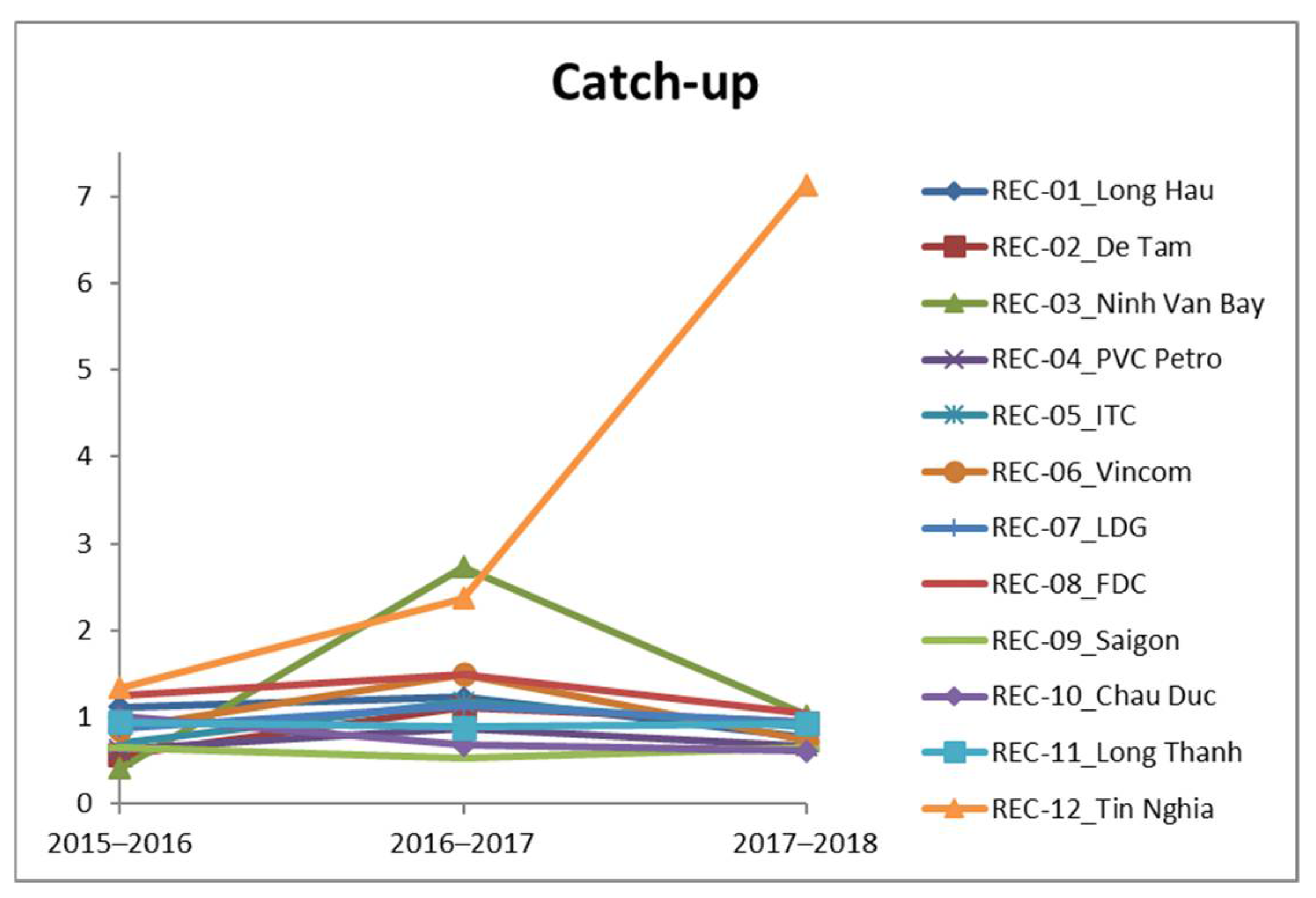
Table 7 and Figure 2 show the efficiency change (catch-up) of the 12 DMUs from 2015–2018. It can be seen that the catch-up score of every DMU has changed the technical efficiency. Some of the DMUs have significant improvement in efficiency (catch-up score above 1). Among the 12 companies, REC-01 (Long Hau), REC-03 (Ninh Van Bay), REC-06 (Vincom), REC-08 (FDC), and REC-12 (Tin Nghia) have an average catch-up index greater than 1. This proves that these DMUs have achieved efficiency. In general, in the period of 2015–2018, there was a fluctuation in the technical efficiency of all DMUs. REC-12 (Tin Nghia) achieved the best efficiency with C = 3.614967, while REC-09 (Saigon) had the worst efficiency performance with C = 0.611249.

Specifically, in the period of 2015–2016, there were four of the 12 DMUs that achieved technical efficiency (average C > 1). REC-12 (Tin Nghia) achieved the most, with C = 1.339522. On the other hand, REC-03 (Ninh Van Bay) had the lowest technical efficiency with C = 0.413726.

Compared to the period of 2015–2016, there was an increase in technical efficiency improvement of enterprises during the years 2016–2017. Eight of the 12 DMUs achieved technical efficiency (average C > 1). REC-03 (Ninh Van Bay) is the most achieved with a C of 2.730939. Moreover, in this period, many other companies achieved high technical efficiency such as REC-01, -02, -03, -05, -06, -07, -08, and REC-12. Meanwhile, REC-09 (Saigon) had the worst efficiency performance.

In the period 2017–2018, there were three DMUs that achieved technical efficiency (average C > 1). This is especially true for the outstanding increase in the score of REC-12 over 2017–2018, with an increase of 532.88% compared to the period of 2015–2016. In contrast, it can be seen that some companies like REC-01, 02, 04, 05, 06, 07, 09, 10, and REC-11 have no progress in improving technical efficiency. REC-10 (Chau Duc) had the worst efficiency performance of C = 0.610438. Therefore, the companies that achieved low performance need to pay attention to their technical aspect to enhance their competitiveness in the market.

4.3.2. Frontier-Shift Index

The frontier-shift index (F) is used for assessing the technological efficiency or efficiency frontier of 12 DMUs between two periods. Investing in production technology will improve labor productivity and directly enhance the competitiveness of enterprises in the same field. In Vietnam, many real estate companies have made high-quality products thanks to new research and technology. In contrast, several companies still have very low performance in technological applications.

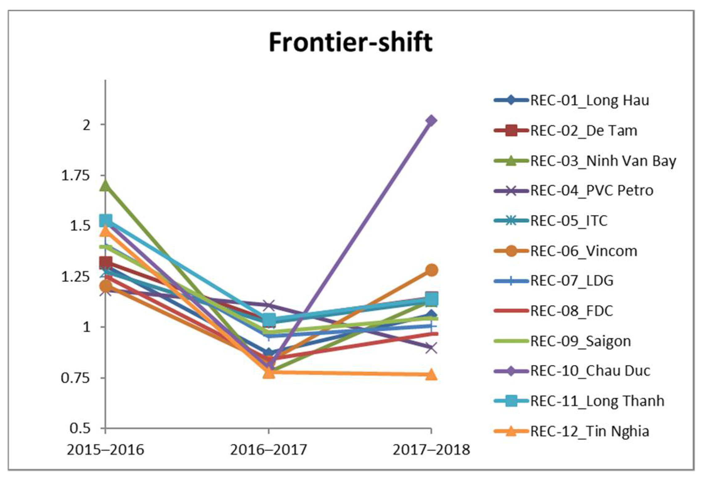
Table 8 and Figure 3 show that the technological efficiency of real estate enterprises tended to decrease in the period of 2016–2017 and increase in the period of 2017–2018. It is estimated that most DMUs enhanced their technology, which overall increasd their technological efficiency. In the period of 2015–2016, all DMUs achieved an average of F > 1. REC-03 (Ninh Van Bay) obtained the best technological efficiency with F = 1.700417. It can be concluded that this DMU achieved significant improvement and advancement in technology in this period.

The results indicate that there are some technological changes between the DMUs. The company with the best performance belongs to REC-10 (Chau Duc). The level of technical change of REC-10 is seen clearly because it has a sharp increase in technical efficiency in the period of 2017–2018 (F = 2.021320) with an approximate growth of 253.16% compared to the period of 2016–2017, where it only increased by 132.65% compared to the period of 2015–2016. It can be seen that REC-10 experienced a sharp decline in the period of 2016–2017 but then regained its technological efficiency in the following period. The remaining DMUs showed relatively stable performance with a slight increase or decrease. Overall, all DMUs have an average frontier-shift score greater than 1, achieving technological progression.

4.3.3. Malmquist Productivity Index

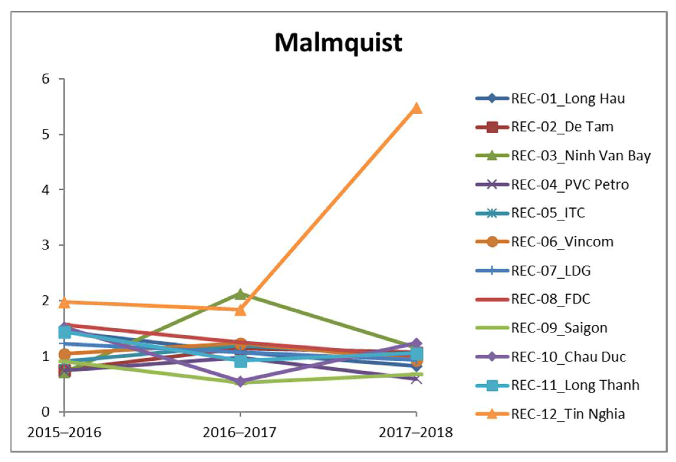
MPI is calculated as the product of technical change and technological change, as can be seen in Equation (16). Hence, to develop and dominate the domestic market, investment in technical and technological improvements is the prerequisite that Vietnamese real estate companies need to focus on. As shown in Table 9 and Figure 4, the average MPI of DMUs is greater than 1. This showed an increase in total factor productivity growth of the 2015–2018 period.

The results show the MPI of real estate companies in Vietnam. Most of them scored more than 1. For example, REC-12 (Tin Nghia) had the largest average productivity index (Malmquist-MPI) change in the period of 2015–2018. From 2015 to 2017, the productivity index of REC-12 decreased slightly from 1.977175 to 1.841234 but then reached a peak of 5.477816 in the period from 2017 to 2018.

In the period 2015–2016, we can see that the difference in total factor productivity among DMUs is considerable. In particular, several DMUs achieved a highly efficient performance, such as REC-01, -06, -07, -08, -10, -11, and REC-12, while others showed opposite trends afterward. REC-03 (Ninh Van Bay) showed the worst performance with MPI = 0.703506 from 2015 to 2016, which shows that the technical and technological investment among the real estate companies is unbalanced. However, it then increased rapidly to 2.129368 from 2016 to 2017; hence, the productivity index still achieved good efficiency in the whole period.

In general, there are two distinct trends in the MPI in the period of 2016–2017. Some of the DMUs have a significant decline compared to the previous period, such as REC-01, -07, -08, -09, -10, -11, and REC-12. In particular, REC-10 (Chau Duc), which had the highest MPI score of 1.52492 in the period of 2015–2016, then a sharp decrease to 0.543632 in the next period before increasing gradually by 1.23389 at the end of the period. This indicates that many real estate companies have not focused on enhancing technical and technological performance, which has led to declining performance. However, this period also witnessed a marked improvement of some manufacturers such as REC-02, -03, -04, -05, and REC-06.

From 2017 to 2018, REC-12 (Tin Nghia) had a significant increase in productivity index changes over the period (MPI = 5.477816); this means during this period, REC-12 has the best productivity proving that this DMU has been very active in keeping up with the real estate market trend during this stage in development. Besides, some DMUs also achieved good performance in terms of factor productivity such as REC-02, -03, -08, -10, -11, and REC-12. In contrast, the REC-01, -04, -05, -06, -07, and REC-09 have an MPI < 1, indicating that these real estate companies tend to reduce productivity. Therefore, these companies need to have specific strategic plans to improve their operational efficiency.

4.4. Results of Malmquist Model (2019–2022)

This part presents the predicted changes in technical efficiency (catch-up index), technological efficiency (frontier-shift index), and total factor productivity of 12 DMUs for the future period of 2019 to 2022. In addition, the comparisons of historical and future performance are shown.

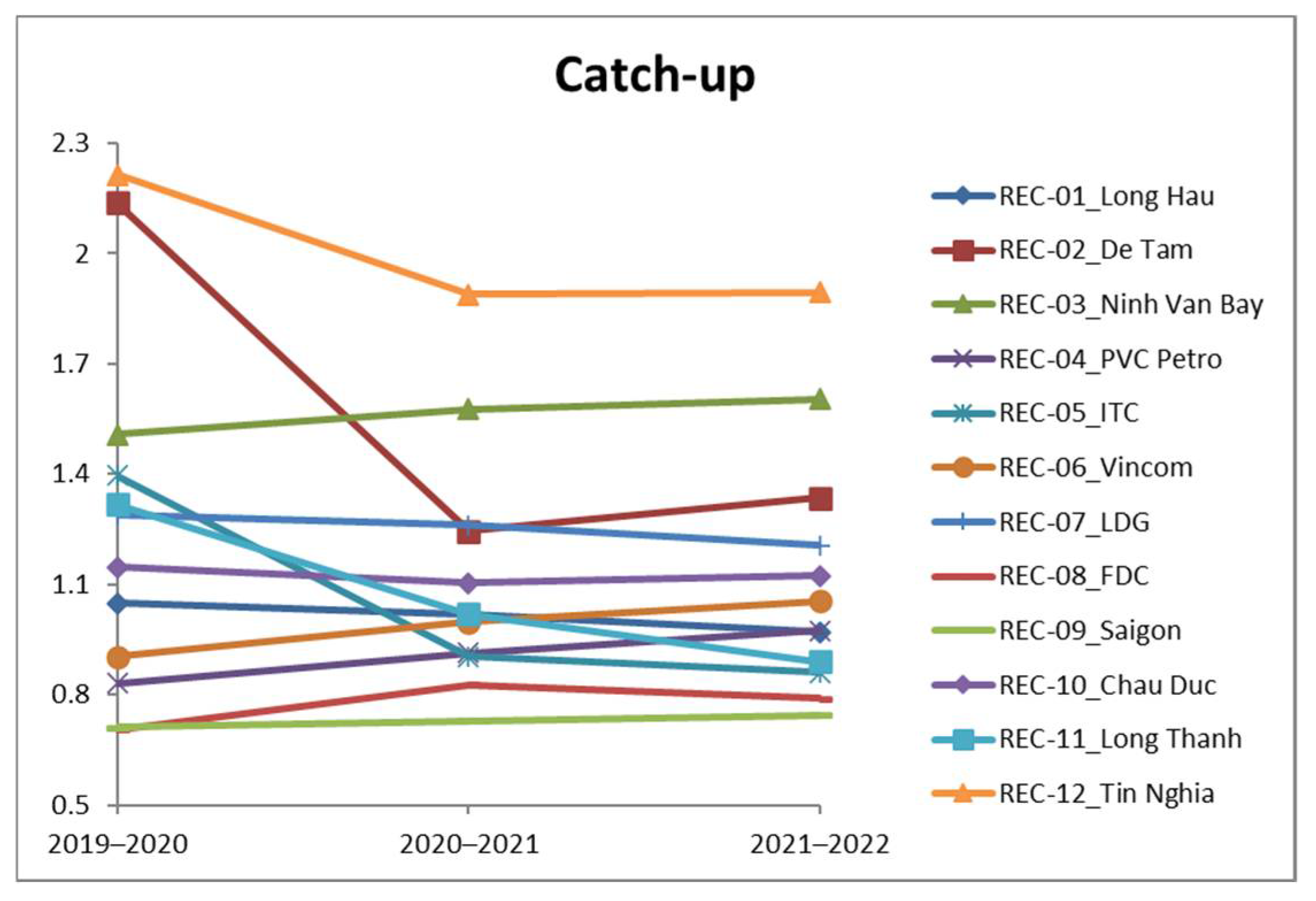
4.4.1. Catch-Up Index

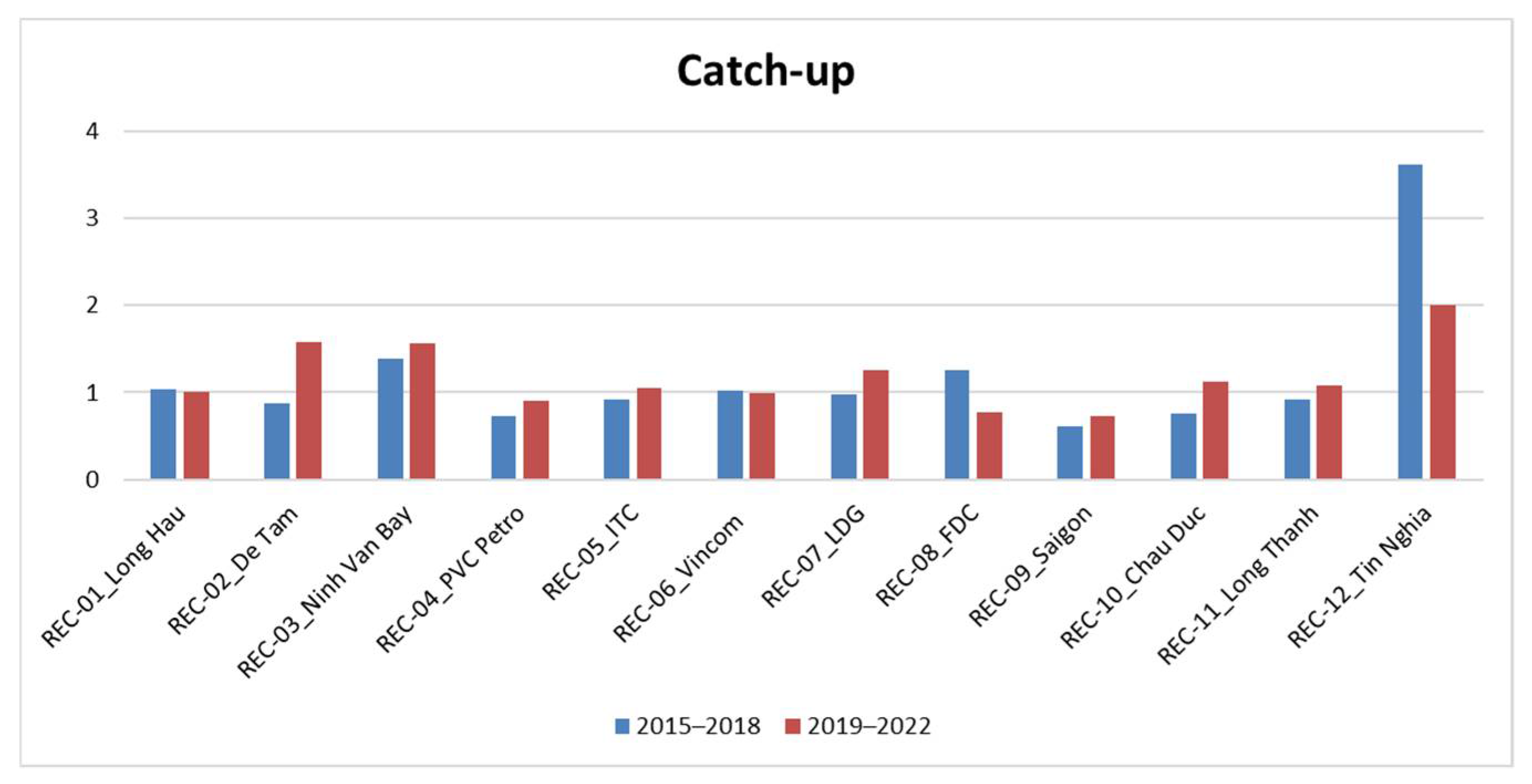
According to

Table 10. Catch-up index (2019–2022).

DMUs	Symbol	2019–2020	2020–2021	2021–2022	Average
REC-01	Long Hau	1.048638	1.018124	0.969749	1.012170
REC-02	De Tam	2.138610	1.245731	1.334692	1.573011
REC-03	Ninh Van Bay	1.506936	1.576088	1.603883	1.562302
REC-04	PVC Petro	0.831035	0.912351	0.974361	0.905916
REC-05	ITC	1.395901	0.902445	0.861053	1.053133
REC-06	Vincom	0.904181	0.998198	1.053601	0.985327
REC-07	LDG	1.290122	1.260970	1.205341	1.252145
REC-08	FDC	0.705192	0.826915	0.789237	0.773781
REC-09	Saigon	0.710973	0.728282	0.743550	0.727602
REC-10	Chau Duc	1.146095	1.102576	1.122614	1.123762
REC-11	Long Thanh	1.318272	1.019893	0.890403	1.076189
REC-12	Tin Nghia	2.214332	1.888561	1.894749	1.999214
Average		1.267524	1.123345	1.120269	1.170379
Max		2.214332	1.888561	1.894749	1.999214
Min		0.705192	0.728282	0.74355	0.727602
SD		0.499389	0.330231	0.344679	0.371327

Note: calculated by the authors.

and Figure 5, the level of the average technical change (catch-up) fluctuates between 0.727602 and 1.999214. It is observed that, in the future period, the real estate enterprises will perform less effectively than in the past period of 2015–2018, as shown by the lower average score. While the average score of the past period of 12 real estate enterprises was 1.176062, that of the future period will be 1.170379. However, there were eight out of 12 companies that will achieve higher efficiency than in the past period, as can be seen in Figure 6. REC-12 will remain the highest score but be far worse than the results of the previous period.

Especially, over the next 4 years, REC-12 (Tin Nghia) is predicted to remain relatively stable for the top position of the technical efficiency with an average of 1.999214. Moreover, REC-02 (De Tam) and REC-03 (Ninh Van Bay) will have a stable efficiency and an average score of greater than 1.5, giving it the second highest position throughout the period. There were also many companies that were predicted to perform better, like REC--01, -03, -05, -07, -10, and REC-11, while REC-04, -06, -08, and -09 will have reduced efficiency. In general, REC-12 (Tin Nghia) was by far the most technically efficient of all 12 companies in almost every period in the entire 4-year period.

From 2019 to 2022, the technical efficiency of REC-02 (De Tam) will drop sharply from 2.138610 to 1.245731 during 2019–2021, but then it will slightly increase to 1.334692 from 2021 to 2022. Likewise, the respective index for the REC-12 (Tin Nghia) also will decrease steeply from 2.214332 to 1.888561 between 2019 and 2021, but then modestly decrease to 1.894749 in 2022. Moreover, REC-01, -05, -07, and REC-11 will reach the highest score from 2019 to 2020, and then these DMUs will decrease throughout the period of 2020–2022. By contrast, REC-03 is predicted to be the lowest score between 2019 and 2020, which will be followed by an increase during 2020–2022. Only REC-10 will slightly decrease, from 1.146095 to 1.102576, during 2020–2021 in the previous stage but then will increase slightly to 1.122614 in the final period of the technical changes. Overall, the eight DMUs above can achieve significant technical efficiency in the future period. Therefore, strategic planners can rely on this research to make a more accurate investment. On the other hand, REC-04 (PVC Petro), REC-06 (Vincom), REC-08 (FDC), and REC-09 (Saigon) will only increase and decrease slightly from 2019 to 2022, with an average less than 1, indicating that its performance decreases. Therefore, the companies need to pay attention to their technical aspect to enhance their competitiveness in this market in the future.

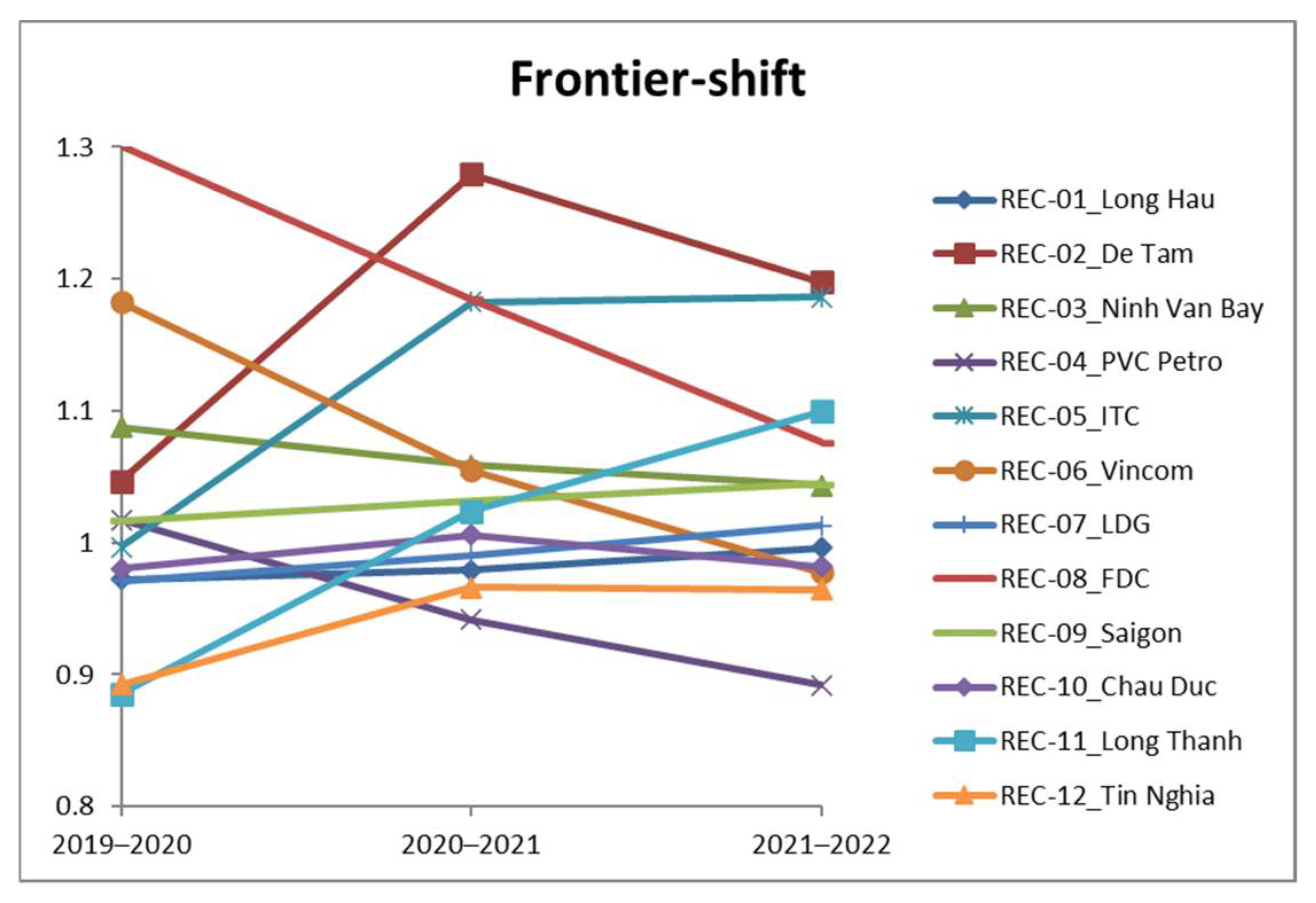
4.4.2. Frontier-Shift Index

Table 11. Frontier-shift (2019–2022).

DMUs	Symbol	2019–2020	2020–2021	2021–2022	Average
REC-01	Long Hau	0.971922	0.979279	0.996110	0.982437
REC-02	De Tam	1.046647	1.279452	1.197869	1.174656
REC-03	Ninh Van Bay	1.087661	1.058733	1.043421	1.063272
REC-04	PVC Petro	1.017075	0.941752	0.891707	0.950178
REC-05	ITC	0.996402	1.182692	1.186114	1.121736
REC-06	Vincom	1.182331	1.055000	0.977638	1.071656
REC-07	LDG	0.971117	0.990437	1.013010	0.991522
REC-08	FDC	1.301262	1.184865	1.076112	1.187413
REC-09	Saigon	1.016941	1.031735	1.044390	1.031022
REC-10	Chau Duc	0.980184	1.005760	0.981857	0.989267
REC-11	Long Thanh	0.885382	1.023607	1.099849	1.002946
REC-12	Tin Nghia	0.892571	0.966333	0.964663	0.941189
Average		1.029125	1.058304	1.039395	1.042274
Max		1.301262	1.279452	1.197869	1.187413
Min		0.885382	0.941752	0.891707	0.941189
SD		0.117152	0.10356	0.089836	0.082873

Note: calculated by the authors.

and Figure 7 illustrate the change in technology (frontier-shift) in the period of 2019–2022. In general, these real estate companies will have relatively stable technological growth, only increasing or decreasing slightly to nearly 1 over the whole period. Most DMUs have frontier-shift indexes higher than 1, which proves that they are actively working to improve the technology applied to their business, except for REC-01, -04, -07, -10, and REC-12 with an average index less than 1. Therefore, these companies need to pay attention to comprehensive investment, especially, in technical aspects to enhance their performance to integrate with the development of the current real estate market.

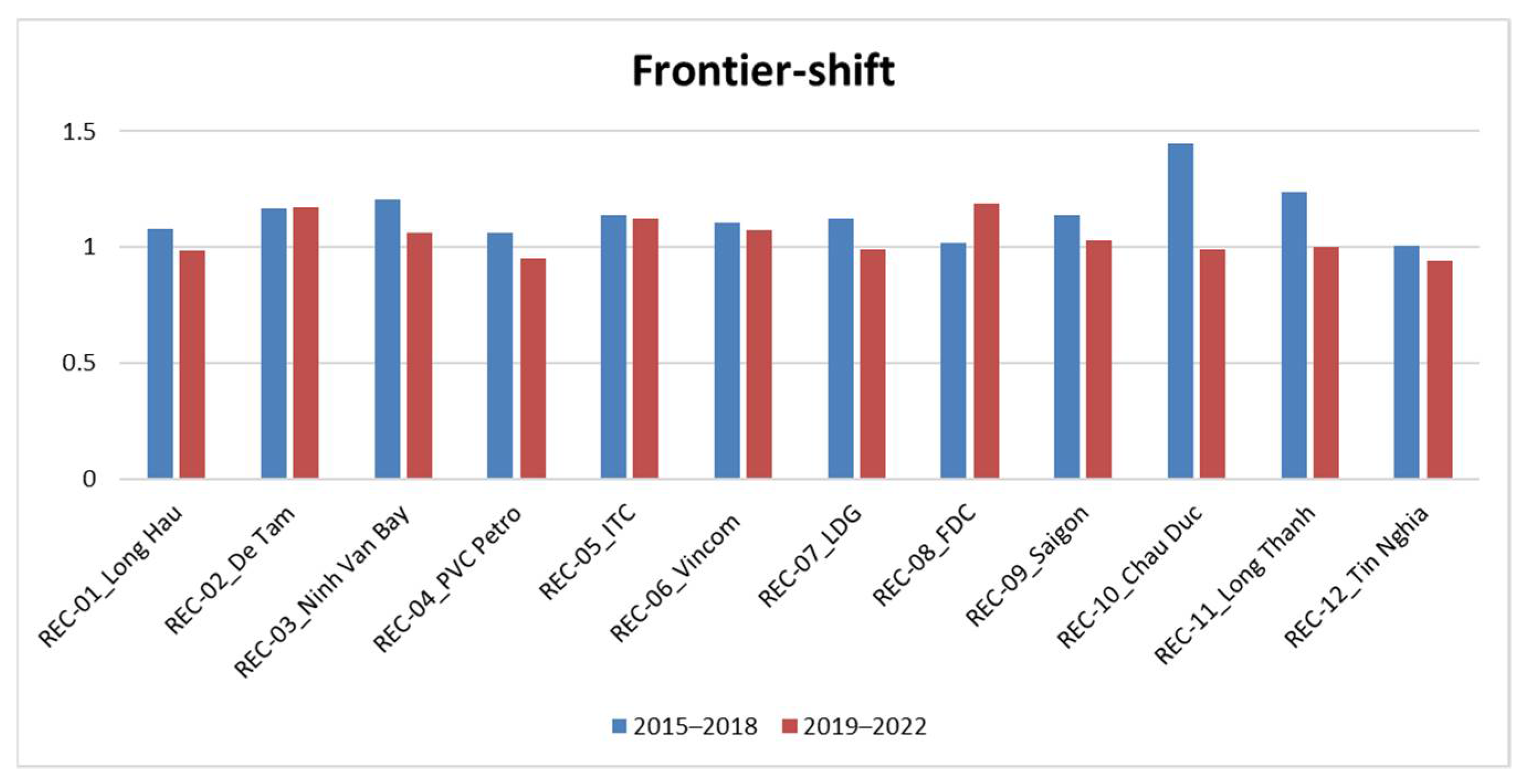
Moreover, in Figure 8, the graph shows the comparison of technological change between the periods of 2015–2018 and 2019–2022. It clearly shows that most DMUs will decrease their efficiency in the future. The average efficiency of REC-10 (Chau Duc) especially decreased sharply by 0.989267 from 1.447864 in the past period. REC-02 (De Tam) and REC-05 (ITC) will remain relatively stable. The remaining DMUs will significantly reduce technological efficiency when compared to those in the period 2015–2018.

4.4.3. Malmquist Productivity Index

Table 12. Malmquist productivity index (2019–2022).

DMUs	Symbol	2019–2020	2020–2021	2021–2022	Average
REC-01	Long Hau	1.019195	0.997028	0.965976	0.994066
REC-02	De Tam	2.238369	1.593853	1.598786	1.810336
REC-03	Ninh Van Bay	1.639035	1.668656	1.673525	1.660405
REC-04	PVC Petro	0.845225	0.859209	0.868845	0.857760
REC-05	ITC	1.390878	1.067314	1.021307	1.159833
REC-06	Vincom	1.069041	1.053100	1.030040	1.050727
REC-07	LDG	1.252860	1.248912	1.221023	1.240932
REC-08	FDC	0.917640	0.979783	0.849307	0.915577
REC-09	Saigon	0.723017	0.751394	0.776557	0.750323
REC-10	Chau Duc	1.123385	1.108927	1.102246	1.111519
REC-11	Long Thanh	1.167174	1.043970	0.979309	1.063484
REC-12	Tin Nghia	1.976449	1.824978	1.827795	1.876407
Average		1.280189	1.183094	1.15956	1.207614
Max		2.238369	1.824978	1.827795	1.876407
Min		0.723017	0.751394	0.776557	0.750323
SD		0.459821	0.336185	0.349545	0.373679

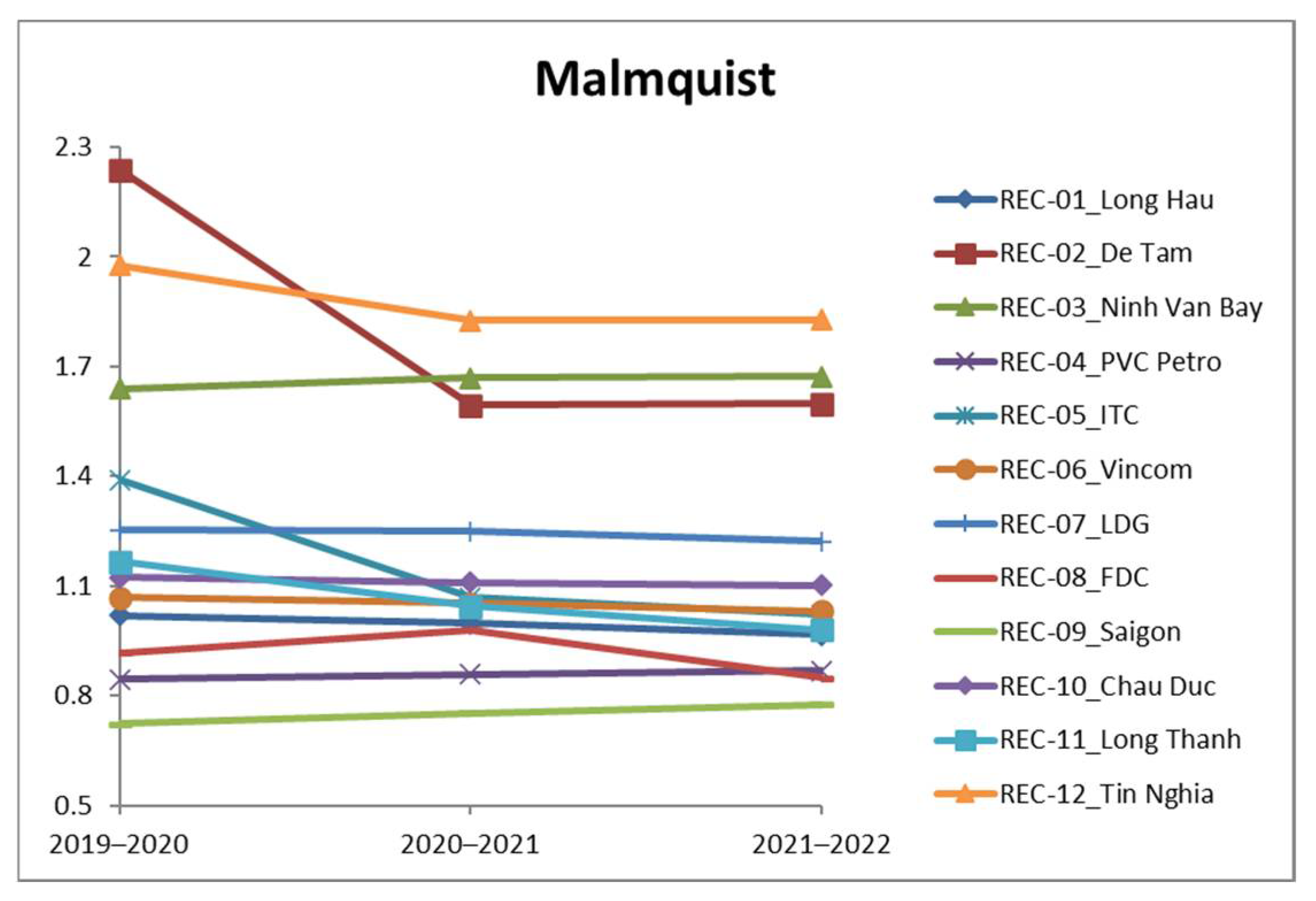
Note: calculated by the authors.

and Figure 9 show the results of the total factor productivity change, which is the most important indicator in the DEA Malmquist model. This index is used to evaluate the future performance of 12 real estate companies. Investors can rely on these predicted overview picture to make an accurate decision. Overall, almost all of these DMUs will have an increase in the productivity index in the future, except for REC-01, -04, -08, and REC-09, which will decrease in efficiency to less than 1. REC-12 (Tin Nghia) productivity index will remain stable in the first position, which is the best performing in all these companies. The next position will be REC-02 (De Tam) with an average of 1.810336, almost equal to the average of REC-12 of 1.876407.

Especially in the next 4-year from 2019 to 2022, the total factor productivity scores of REC-01, -02, -05, -06, -07, -08, -10, -11, and REC-12 will decline gradually while REC-03, -04, and REC-09 will increase slightly over entire the period. REC-09 (Saigon) was also by far the lowest average score of all the 12 companies (MPI = 0.750323). In addition, the REC-02 (De Tam) and REC-12 (Tin Nghia) will have a sharp drop during 2019–2021, but then a slight increase in the final period. REC-02 (De Tam) dropped significantly from 2.238369 to 1.593853 during 2019–2021. REC-08 (FDC) showed the opposite, increasing afterward. This company will gradually decline from 2020–2021, which will be followed by a slight increase from 2021 to 2022. The data suggest that this company needs to reconsider the application of technology to help keep good technological efficiency.

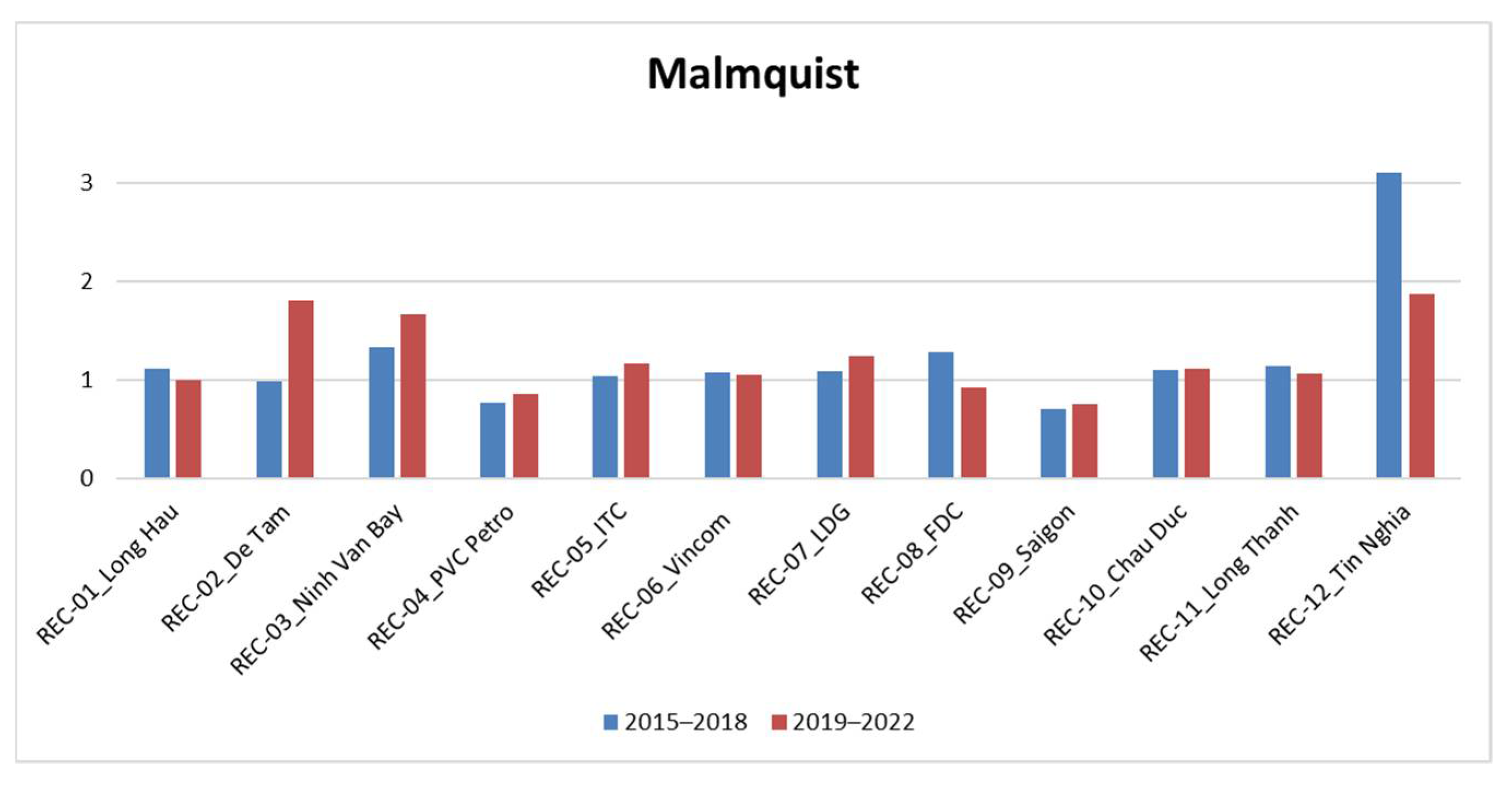
As a result, the graph in Figure 10 compares productivity changes of the companies between the 2015–2018 period and the 2019–2022 period. Overall, the efficiency of multiple companies will decrease remarkably when compared to those in the past period. The REC-12 (Tin Nghia) will still reach the highest score of 12 companies but in the future period, it will be a significant reduction. This was suggested that this company needs to accelerate and apply the correct production processes to help the company grow more and more.

5. Discussions

This section discusses the results of the research and presents the management implications as well as recommendations and suggestions for future studies. First, trends in real estate companies are hard to predict because the real estate market is greatly influenced by not only economic development but also technology. The Grey model, GM (1,1), requires not only minimal data but also the best of all models available at short-term predictions. This has been proven by many previous studies of Grey’s theory [41,42]. The average MAPE of all DMUs was 9.756% and rated as good (MAPE < 10%), which proved that the Grey model of GM (1,1) is suitable for this research. Consequently, the researcher used the DEA Malmquist model to provide an insight into the performance of these DMUs for both the past and the future of the top 12 real estate companies in Vietnam.

In summary, two-side productivity evaluation comparison of all DMUs is shown in Figure 11. The average score of real estate companies in Vietnam fluctuated from 2015 to 2018. This result shows that most DMUs tended to increase productivity, especially REC-12 (Tin Nghia), which achieved the best performance in all companies, while REC-02 (De Tam), REC-04 (PVC Petro), and REC-09 (Saigon) reduced its productivity. This implies that these three companies should focus more on the technical efficiency and technological efficiency of their businesses every year. Furthermore, according to the forecasts for their performances in the period of 2019–2022, almost all DMUs will have an increase in their total factor productivity indexes. Although REC-12 (Tin Nghia) with MPI will be reduced compared to the period of 2015–2018, in general, REC-12 (Tin Nghia) will still achieve the best performance in all companies studied. From the performance of each business year by year, this can help managers identify a company’s weaknesses or strengths to change its strategy. The burden of how to improve efficiency, competitiveness, and expand business size is placed on the shoulders of business managers. Based on MPI, companies with MPI less than 1 should proactively monitor, improve technology, or use any other method that improves future productivity. For companies whose productivity index is always greater than 1, this shows the potential for a profitable investment. Investors can rely on that to devise themselves with a sound investment strategy.

According to the financial representative in Vietnam [43,44], due to the COVID-19 era, the real estate markets are forecasting lower profits in the following years, such as REC-12 (Tin Nghia) expects its revenue to reach 166 billion VND, down 24 percent against 2019, and pre-tax profit to touch 93 billion VND, down 19 percent each year. In the fight against this global pandemic, many major real estate investors in Vietnam are considering integrating more 4.0 technologies to develop a clear competitive advantage [45]. The model’s results aim to provide comprehensive managerial implications to the real estate industry in Vietnam for assessing their past-present-future comparative analysis with other competitors, especially in the COVID-19 pandemic, since it has been found that the pandemic has had a significant effect on this industry. The authors expect that the results will reflect the current situation of the real estate industry with respect to technical and technological efficiency. Hence, the insights of this paper could help managers, investors, and policymakers improve their decision-making process and find out key performance indexes to enhance real estate toward sustainable development.

6. Conclusions

By implementing performance prediction and evaluation of the real estate industry, the combined two-stage model is suggested to analyze the changes in technical efficiency (catch-up index), technological effect (frontier-shift index), and total productivity factor. The proposed model was tested using a case study of the top 12 real estate companies in Vietnam. In the model, input factors included total assets, cost of sales, and cost of goods sold, while total revenue and gross profit were considered as output factors. The findings of the paper were that, in the first-stage period of 2015–2018, the drastic technical efficiency changes in some companies were observed, even though the technological efficiency was stable in the period. In the second-stage period of 2019–2022, most real estate companies achieved a relatively stable total productivity factor.

To the best of the author’s knowledge, a two-stage model for the prediction and evaluation of real estate management in Vietnam by integrating GM (1,1) and DEA Malmquist model to predict and evaluate the performance of real estate companies has never been reported. This lack attracted our attention. Therefore, this paper aims to provide an evaluation method for businesses to find out key factors that impact their success in the real estate industry. This mathematical method helps investors as well as strategic suppliers minimize errors and risks in decision making. This method can also be used in many different industries to help expand its scope of research. Therefore, this study will serve as a document to help policymakers make accurate and reasonable decisions. They need to adjust and revise their strategy if they foresee future results.

Although this research discusses the effectiveness of real estate companies in Vietnam, it still has limitations. Firstly, future studies should focus on finding new assessment factors that can impact the business performance of real estate such as labor force, personal savings, and exchange rate. Secondly, there are only 12 DMUs in this paper; hence, future studies should provide additional DMUs that will improve the accuracy of this research.

References

- Financial Resources to Promote Vietnam’s Real Estate Market. 2019. Available online: http://tapchitaichinh.vn/thi-truong-tai-chinh/nguon-luc-tai-chinh-thuc-day-thi-truong-bat-dong-san-viet-nam-phat-trien-310970.html (accessed on 1 August 2020).
- Vietnam’s Real Estate Market and Its Impact Factors. 2019. Available online: http://tapchitaichinh.vn/thi-truong-tai-chinh/thi-truong-bat-dong-san-viet-nam-va-nhung-yeu-to-tac-dong-310779.html (accessed on 5 November 2019).
- Viet Nam Real Estate Report from Now to 2020. 2019. Available online: https://batdongsanexpress.vn/bao-cao-tinh-hinh-bat-dong-san-viet-nam-tu-nay-den-nam-2020.html (accessed on 31 October 2019).
- Real Estate Express. Available online: https://batdongsanexpress.vn/bao-cao-tinh-hinh-thi-truong-bat-dong-san-viet-nam-sau-giai-doan-dong-bang.html (accessed on 31 October 2019).
- Vietnam Real Estate Market 2020 during COVID-19. Available online: http://baochinhphu.vn/Thi-truong/Dan-dat-dong-tien-dau-tu-bat-dong-san-hau-COVID/415109.vgp (accessed on 25 November 2010).
- Charnes, A.; Cooper, W.W.; Rhodes, E. Measuring the efficiency of decision-making units. Eur. J. Oper. Res. 1978, 2, 429–444. [Google Scholar] [CrossRef]
- Drake, L.; Hall, M.J. Efficiency in Japanese banking: An empirical analysis. J. Bank. Financ. 2003, 27, 891–917. [Google Scholar] [CrossRef]
- Bayyurt, N.; Gokhan, D.U.Z.U. Performance measurement of Turkish and Chinese manufacturing firms: A comparative analysis. Eur. J. Bus. Econ. 2008, 1, 71–83. [Google Scholar]
- Wang, C.N.; Li, K.Z.; Ho, C.T.; Yang, K.L.; Wang, C.H. A model for candidate selection of strategic alliances: Case on industry of department store. In Proceedings of the Second International Conference on Innovative Computing, Informatio and Control (ICICIC 2007), Kumamoto, Japan, 5–7 September 2007; p. 85. [Google Scholar]
- Färe, R.; Grosskopf, S.; Lindgren, B.; Roos, P. Productivity changes in Swedish pharmacies 19801989: A non-parametric approach. J. Product. Anal. 1992, 3, 85101. [Google Scholar]
- Chang, D.S.; Kuo, L.C.R.; Chen, Y.T. Industrial changes in corporate sustainability performance–An empirical overview using data envelopment analysis. J. Clean. Prod. 2013, 56, 147–155. [Google Scholar] [CrossRef]
- Wu, W.Y.; Tsai, H.J.; Cheng, K.Y.; Lai, M. Assessment of intellectual capital management in Taiwanese IC design companies: Using DEA and the Malmquist productivity index. RD Manag. 2006, 36, 531–545. [Google Scholar] [CrossRef]
- Egilmez, G.; McAvoy, D. Benchmarking road safety of US states: A DEA-based Malmquist productivity index approach. Accid. Anal. Prev. 2013, 53, 55–64. [Google Scholar] [CrossRef]
- Vassdal, T.; Sørensen Holst, H.M. Technical progress and regress in Norwegian salmon farming: A Malmquist index approach. Mar. Resour. Econ. 2011, 26, 329–341. [Google Scholar] [CrossRef]
- Deng, J.L. Control problems of grey systems. Syst. Control Lett. 1982, 1, 288–294. [Google Scholar]
- Trivedi, H.V.; Singh, J.K. Application of grey system theory in the development of a runoff prediction model. Biosyst. Eng. 2005, 92, 521–526. [Google Scholar] [CrossRef]
- Wong, H.L.; Shiu, J.M. Comparisons of fuzzy time series and hybrid Grey model for non-stationary data forecasting. Appl. Math. Inf. Sci. 2012, 6, 409–416. [Google Scholar]
- Wang, C.N.; Le, T.M.; Nguyen, H.K.; Ngoc-Nguyen, H. Using the Optimization Algorithm to Evaluate the Energetic Industry: A Case Study in Thailand. Processes 2019, 7, 87. [Google Scholar] [CrossRef] [Green Version]
- Yuan-yuan, J.; Li-xin, L.; En-yuan, L. Analysis on the efficiency of real estate industry based on DEA in Ningbo City. In Proceedings of the 2010 International Conference on Management Science & Engineering 17th Annual Conference Proceedings, Melbourne, VIC, Australia, 24–26 November 2010; pp. 1632–1637. [Google Scholar]
- Ge, H.; Guo, Y.W. Efficiency of listed real estate companies in China based on the two-stage DEA. In Proceedings of the 2014 International Conference on Management Science & Engineering 21th Annual Conference Proceedings, Helsinki, Finland, 17–19 August 2014; pp. 1313–1318. [Google Scholar]
- Soetanto, T.V.; Fun, L.P. Performance evaluation of property and real estate companies listed on Indonesia Stock exchange using data envelopment analysis. J. Manaj. Dan Kewirausahaan 2014, 16, 121–130. [Google Scholar] [CrossRef] [Green Version]
- Morita, H.; Avkiran, N.K. Selecting inputs and outputs in data envelopment analysis by designing statistical experiments. J. Oper. Res. Soc. Jpn. 2009, 52, 163–173. [Google Scholar]
- Data Collection. Available online: https://vietstock.vn/ (accessed on 31 October 2019).
- Qi, W.; Jia, S. The empirical study on productivity of Chinese real estate enterprises based on DEA-based Malmquist model. In Proceedings of the 2010 Second International Conference on Communication Systems, Networks and Applications, Hong Kong, China, 29 June–1 July 2010; pp. 248–251. [Google Scholar]
- Peng Wong, W.; Gholipour, H.F.; Bazrafshan, E. How efficient are real estate and construction companies in Iran’s close economy? Int. J. Strateg. Prop. Manag. 2012, 16, 392–413. [Google Scholar] [CrossRef] [Green Version]
- Harun, S.L.; Tahir, H.M.; Zaharudin, Z.A. Measuring efficiency of real estate investment trust using data envelopment analysis approach. In Proceedings of the Fifth Foundaition of Islamic Finance Conference, Langkawi, Malaysia, 9–11 July 2012; pp. 1–12. [Google Scholar]
- Wang, Y.; Zhu, Y.; Jiang, M. Efficiency evaluation of listed real estate companies in China. In The Strategies of China’s Firms; Chandos Publishing: Cambridge, UK, 2015; pp. 89–107. [Google Scholar]
- Chen, Q.; Li, F. Empirical analysis on efficiency of listed real estate companies in China by DEA. Ibusiness 2017, 9, 49. [Google Scholar] [CrossRef] [Green Version]
- Ahmed, A.A.; Mohamad, A. Data envelopment analysis of efficiency of real estate investment trusts in Singapore. Int. J. Law Manag. 2017, 59, 826–838. [Google Scholar] [CrossRef]
- Atta Mills, E.F.E.; Baafi, M.A.; Liu, F.; Zeng, K. Dynamic operating efficiency and its determining factors of listed real-estate companies in China: A hierarchical slack-based DEA-OLS approach. Int. J. Financ. Econ. 2020, 10, 1–25. [Google Scholar] [CrossRef]
- Kayacan, E.; Ulutas, B.; Kaynak, O. Grey system theory-based models in time series prediction. Expert Syst. Appl. 2010, 37, 1784–1789. [Google Scholar] [CrossRef]
- Julong, D. Introduction to grey system theory. J. Grey Syst. 1989, 1, 1–24. [Google Scholar]
- Tseng, F.-M.; Yu, H.-C.; Tzeng, G.-H. Applied hybrid grey model to forecast seasonal time series. Technol. Soc. Chang. 2001, 67, 291–302. [Google Scholar] [CrossRef]
- Wang, C.N.; Tibo, H.; Duong, D.H. Renewable Energy Utilization Analysis of Highly and Newly Industrialized Countries Using an Undesirable Output Model. Energies 2020, 13, 2629. [Google Scholar] [CrossRef]
- Lewis, C.D. International and Business Forecasting Methods; Routlege: London, UK, 1982. [Google Scholar]
- Wang, C.N.; Hsu, H.P.; Wang, Y.H.; Nguyen, T.T. Eco-Efficiency Assessment for Some European Countries Using Slacks-Based Measure Data Envelopment Analysis. Appl. Sci. 2020, 10, 1760. [Google Scholar] [CrossRef] [Green Version]
- Färe, R.; Grosskopf, S.; Norris, M.; Zhang, Z. Productivity growth, technical progress, and efficiency change in industrialized countries. Am. Econ. Rev. 1994, 84, 66–83. [Google Scholar]
- Wang, C.N.; Nguyen, N.T.; Tran, T.T. Integrated DEA models and grey system theory to evaluate past-to-future performance: A case of Indian electricity industry. Sci. World J. 2015, 638710. [Google Scholar] [CrossRef] [Green Version]
- Liu, F.H.F.; Wang, P.H. DEA Malmquist productivity measure: Taiwanese semiconductor companies. Int. J. Prod. Econ. 2008, 112, 367–379. [Google Scholar] [CrossRef]
- Wang, C.-N.; Dang, T.-T.; Nguyen, N.-A.-T.; Le, T.-T.-H. Supporting Better Decision-Making: A Combined Grey Model and Data Envelopment Analysis for Efficiency Evaluation in E-Commerce Marketplaces. Sustainability 2020, 12, 10385. [Google Scholar] [CrossRef]
- Le, T.N.; Wang, C.N. The integrated approach for sustainable performance evaluation in value chain of Vietnam textile and apparel industry. Sustainability 2017, 9, 477. [Google Scholar] [CrossRef] [Green Version]
- Wang, C.N.; Tsai, T.T.; Hsu, H.P.; Nguyen, L.H. Performance evaluation of major asian airline companies using DEA window model and grey theory. Sustainability 2019, 11, 2701. [Google Scholar] [CrossRef] [Green Version]
- Industrial Parks Forecast Lower Profits Due to COVID-19 (Vnexplorer). Available online: https://vnexplorer.net/industrial-parks-forecast-lower-profits-due-to-covid-19-a202023040.html?fbclid=IwAR32gj9yPg4PdAB8mbrbLgzOlrMy5b7JQ7ha5IqzkZh8GBQYRMIq-1yoLaM (accessed on 13 January 2020).
- Financial Intel on Vietnam. Available online: https://fintel.vn/tin-nghia-industrial-park-will-pour-1300-billion-vnd-to-invest-in-the-industrial-park/?fbclid=IwAR1WfPlpF7JLgJtzVuL1SPqZVJuN5ccttBt4J8yVizH2XOeCfaULmRwPQHs (accessed on 13 January 2020).
- Technology Shows Its Value to Property Management During Covid-19. Available online: https://www.savills.com.vn/insight-and-opinion/savills-news/186366-0/technology-shows-its-value-to-property-management-during-covid-19?fbclid=IwAR0Oi_2KzXtHhlLun7ihu6co3GEq6sUXGW0gHeOyhjwRzow_sx8CeeDVx7s (accessed on 13 January 2020).