
Discrete Optimization: The Case of Generalized BCC Lattice
by
 , , and
Gergely Kovács
1,† ,
,
Benedek Nagy
2,†,
Gergely Stomfai
3,†,
Neşet Deniz Turgay
2,*,† and
and
Béla Vizvári
4,† 1
Department of Methodology of Applied Sciences, Edutus University, 2800 Tatabánya, Hungary
2
Department of Mathematics, Faculty of Arts and Sciences, Eastern Mediterranean University, Famagusta 99628, North Cyprus, Turkey
3
ELTE Apáczai Csere János High School, 1053 Budapest, Hungary
4
Department of Industrial Engineering, Eastern Mediterranean University, Famagusta 99628, North Cyprus, Turkey
*
Author to whom correspondence should be addressed.
†
These authors contributed equally to this work.
Mathematics 2021, 9(3), 208; https://doi.org/10.3390/math9030208
Submission received: 26 November 2020
/
Revised: 5 January 2021
/
Accepted: 18 January 2021
/
Published: 20 January 2021
(This article belongs to the Special Issue Mathematical Methods for Operations Research Problems)
Abstract
:Recently, operations research, especially linear integer-programming, is used in various grids to find optimal paths and, based on that, digital distance. The 4 and higher-dimensional body-centered-cubic grids is the nD () equivalent of the 3D body-centered cubic grid, a well-known grid from solid state physics. These grids consist of integer points such that the parity of all coordinates are the same: either all coordinates are odd or even. A popular type digital distance, the chamfer distance, is used which is based on chamfer paths. There are two types of neighbors (closest same parity and closest different parity point-pairs), and the two weights for the steps between the neighbors are fixed. Finding the minimal path between two points is equivalent to an integer-programming problem. First, we solve its linear programming relaxation. The optimal path is found if this solution is integer-valued. Otherwise, the Gomory-cut is applied to obtain the integer-programming optimum. Using the special properties of the optimization problem, an optimal solution is determined for all cases of positive weights. The geometry of the paths are described by the Hilbert basis of the non-negative part of the kernel space of matrix of steps.
1. Introduction
In digital geometry, by modeling the world on a grid, path-based distances are frequently used [1,2]. They allow to apply various algorithms of computer graphics and image processing and analysis, e.g., distance transformation [3]. Non traditional grids (related to various crystal structures) have various advantages over the traditional rectangular grids, e.g., having better packing density.
The face-centered cubic (FCC) and body-centered cubic (BCC) lattices are very important non-traditional grids appearing in nature. While the FCC grid is obtained from the cubic grid by adding a point to the center of each square face of the unit cubes, in the BCC grid, the additional points are in the centers of the bodies of the unit cells. Both FCC and BCC are point lattices (i.e., grid vectors point to grid points from any point of the grid). In this paper, we concentrate on the BCC grid and its higher dimensional generalizations. The BCC grid can be viewed as the union of the cubic lattices (the body-centers of the above-mentioned unit cubes form also a cubic lattice). The points located in edge-connected corners of a cube are called 2-neighbors, these points are from the same cubic lattice, while a corner and the body-center of a unit cell are 1-neighbors, as they are the closest neighbor point pairs in the 3D BCC lattice.
There is a topological paradox with the rectangular grids in every dimension, that can be highlighted as follows: considering a usual chessboard, the two diagonals contain different color squares, they go through on each other without a crossing, i.e., without a shared pixel. This is due to the fact that neighbor squares of a diagonal share only a corner point, and no side. One of the main advantages of the BCC grid is, that there are only face neighbor voxels, i.e., if two Voronoi bodies of the grid share at least one point on their boundary, then they share a full face (either a hexagon or a square). In this way, in the BCC grid, the topological paradox mentioned above cannot occur. The inner and outer part of the space is well-defined for any object built up by voxels of the BCC grid. Another important reason considering the BCC grid is its well applicability in graphical reconstruction.
The BCC lattice has been proven to be optimal for sampling spherically band-limited signals.
To perfectly reconstruct these signals from their discrete representations, around fewer samples per unit volume have to be taken on a BCC grid than on an equivalent cubic grid. When the same number of samples is used with equivalent filters for resampling, a BCC-sampled volume representation ensures much higher quality of reconstruction than a cubic-sampled representation does [4,5,6].
Higher dimensional variants of FCC and BCC grids can also be defined and they have both theoretical and practical interest [7]. As their finite segments can be seen as graphs, they could also be used to build special architecture processor or computer networks. The BCC grid has the advantage that, independent of the dimension, exactly two types of neighborhoods are defined and thus, it allows relatively simple simulations (e.g., random walks) and computations. We note here that in the 4 dimensional extension of the BCC grid, the two types of neighbors have exactly the same Euclidean distance and in higher dimension, actually, the 2-neighbors of a point are closer than its 1-neighbor.
Concerning path-based (in grids, they are also called digital) distances, one of the simplest, but on the other hand, very practical and well applicable choices is to use chamfer distances [3]. These distances are, in fact, weighted distances based on various (positive) weights assigned to steps to various types of neighbors. These distances are studied in various grids [7,8,9,10] both with theoretical and practical analysis and also in connection with other fields including approximations of the Euclidean distance [11,12] and various other applications.
In this paper, similar to what we have used in other nontraditional grids (see, e.g., [8,13,14] for analogous results on the semi-regular Khalimsky grid and on the regular triangular grid), we use the tools for operation research to find shortest paths (optimal solution with the terminology of operational research) between any two points. Of course, shortest (also called minimal) paths can be found in various ways, for arbitrary graphs one may use Dijkstra algorithm [15]. However, the grids we use are much more structured than arbitrary graphs as we can refer to the vertices of the graph (points of the grid) by their coordinates. Our method gives explicit formulae for the shortest paths; in this way, our method is more efficient than the application of the Dijkstra algorithm for the grids. This efficiency is obtained by the mathematical analysis of the algorithms.
Since our approach, by using operational research techniques in the field of digital geometry is not common, in the next section we describe our grids and in Section 3 we recall briefly some basic concepts of the field operations research that we need for our work. Further, in Section 4 we represent the shortest path problem on the higher dimensional () BCC grids as an integer programming problem. After filtering the potential bases in Section 5, the optimal solutions are determined in Section 6. Then, in Section 7, the Gomory cut is applied to ensure integer solution. We also give some details on the Hilbert bases of rational polyhedral cones in Section 8. Finally, the paper is concluded in Section 9.
2. The BCC Grid and Its Extensions to Higher Dimensions
Based on a usual description of the BCC grid, we can give the following definitions used throughout of this paper. Let us consider the dimensional digital space , especially, only the points that are represented by either only even or only odd coordinates: is a subset of such that it includes exactly the points if and only if : the parity of all coordinates of x are the same}.
Note that is in fact the square grid with one of its unusual representations called 2D diamond grid/diagonal-square grid and is the original BCC grid, however, in this paper we use mostly and its higher dimensional generalizations.
These grids can be seen as the union of two m dimensional (hyper)cubic (also called rectangular) grids, they are referred as the even and odd (sub)lattices of the grid, based on the parity of the coordinates of their points.
There are two types of usually defined neighborhoods on : We say that the points and are 1-neighbors if and only if for every . These points of are closest neighbors in Euclidean sense if . Moreover, in each dimension, the 1-neighbor points are the closest point pairs containing points from both the even and odd sublattices. Two points and of the same sublattice are 2-neighbors if and only if there is exactly one such that and the points agree on all other coordinate values, i.e., for every , the equation holds. In case , the 2-neighbor points are the second closest point pairs of . However, in dimension 4, the Euclidean distance of the two types of neighborhood relation coincide, while in higher dimensions () the 2-neighbors are closer than the 1-neighbors in Euclidean sense.
Since we have two types of neighbors, we may use different weights for them in chamfer distances. The positive weights of the steps between 1- and 2-neighbors are denoted by w and u in this paper, respectively. We will use the term neighbor for both including 1- and 2-neighbors, and the term step as step from a point to one of its neighbors.
Then, the chamfer distance (also called weighted distance, and in this paper, we will refer to it simply with the term distance), of two points of the grid is defined as the weight of (one of the) smallest weighted path(s) between them, where a path is built up by steps to neighbor points.
Further, each of the mentioned grids is a point lattice, i.e., they are closed under addition of grid vectors. Based on that, when we look for a shortest path between two grid-points, w.l.o.g, we may assume that one of the points is the origin described by the m dimensional zero vector.
3. Theoretical Bases from Linear and Integer Programming
3.1. The Linear Programming Problem
The problem of linear programming is an optimization problem such that the mathematical form of both the objective function and the constraints are linear. The standard form of the problem is as follows:
where G is an matrix, h is an m dimensional vector, f is an n dimensional vector of constants, and x is the n dimensional vector of variables. Notice that the non-negativity constraints are linear inequalities. In the practice, it is necessary to allow that some constraints are inequalities and some variables are “free”, i.e., they may have positive, zero, and negative values as well. It is easy to see that any optimization problem with linear constraints and objective function can be transformed to the standard form by embedding the problem into a higher dimensional space.
3.2. The Simplex Method and Its Geometric Content
The linear programming and its first general algorithm, the simplex method was discovered by George Dantzig in 1947. However, it was published only in 1949 [16]. The simplex method is still in intensive use by professional solvers. It also gives a complete description of the convex polyhedral sets. This theory is summarized based on the book [17]. The author is well-known for the international operations research community as he obtained the EURO Gold Medal in 2003. However, this early book of him is not known for the international scientific community, although it is the best book written on the geometry of linear programming by the authors opinion.
A convex polyhedral set is the intersection of finitely many half-spaces. Notice that the ball is the intersection of infinitely many half-spaces. What is called 0-dimensional facet or corner point in the usual geometry, is called extreme point in this theory. A point is an extreme point of the polyhedral set if it is the only intersection point of the polyhedral set and a supporting hyperplane. Notice that all surface points of the ball are extreme points in this sense, as they are the intersection points of the ball and the tangent plane. The extreme points of the polyhedral set of the linear programming problem are the basic feasible solutions. For the sake of simplicity, assume that the rank of matrix G is m. Let B be a subset of the columns of G such that the vectors of B form a basis. The matrix formed from the elements of B is an matrix. It is also denoted by B. Assume that matrix G and vector x are partitioned accordingly, i.e., , and . The basic solution of basis B is obtained if x satisfies the equation system and its part is 0. It can be obtained as follows:
Hence,
Thus, the part of the basic solution is . The basic solution is feasible if .
The simplex method starts from an extreme point of the polyhedral set, i.e., from a basic feasible solution. The algorithm moves from here to a neighboring extreme point. Two extreme points are neighboring, if a one dimensional edge of the polyhedral set connects them. The value of the objecting function in the selected neighboring extreme point is at least as good as in the current extreme point. This procedure is repeated. It stops if the current extreme point is an optimal solution. There are important consequences. One is that if an optimal solution exists, then at least one basic feasible solution is optimal. The other one is as follows: Let the set of the extreme points of the polyhedral set be the set of vertices of an undirected graph. Two vertices are connected by an edge if and only if an edge of the polyhedral set connects them. This graph is a connected graph as (i) there is no restriction on the starting point and (ii) every other extreme point can be optimal, because its support plane determines a linear objective function such that only this extreme point is optimal solution.
The optimality condition of the simplex method is as follows. Let be the vector consisting of the basic components of the objective function. The current basic feasible solution is optimal, if the inequality
holds for all non-basic columns of G. In other words, (2) must hold for all columns in N. If the inequality (2) is violated by a column , then can replace a vector of the basis such that the objective function value either improves or remains the same. The latter case will be excluded by the strict inequalities assumed among the data of the minimal path problem, see below. The replacement can also show that the problem is unbounded. However, this case is also excluded by the assumption of the step lengths.
3.3. The Gomory Cut
Gomory’s method of integer programming is based on the observation that the basic variables are expressed by the other variables in the form of the equation system (1). Assume that one of these equations is
where K is the index set of the non-basic variables. Assume further on, that is non-integer. It is the current value of the integer variable . Let be the fractional part of the coefficient, i.e., the fractional part of
Let us substitute these quantities into the equation. If the equation is rearranged such that all terms which are integers for sure, are in the left-hand side, the new form of the equation is obtained as follows:
Hence,
All the coefficients of this relation are between 0 and 1. Thus the two sides can be congruent only if the value of the right-hand side is in the set . Hence, the inequality
must be satisfied. The summation in (3) goes for the non-basic variables. The value of the non-basic variables is 0 in the basic solution. Thus, this inequality is not satisfied by the current basic feasible solution as the values of the variables in the sum are all 0. This inequality is the Gomory cut.
4. The Integer Programming Model and Its Linear Programming Relaxation
Many problems of combinatorial optimization are actually integer programming problems. The shortest path problem in a finite graph has also its integer programming version. A grid can be represented by an infinite graph. Therefore, the integer programming model is different.
The matrix of the steps of the 4-dimensional BCC grid are as follows:
The matrix of the 4D BCC grid, the vectors represent steps between two neighbor points of the same sublattice (2-neighbors), while the vectors represent diagonal steps, i.e., steps between neighbor points of different sublattices (1-neighbors).
This matrix is denoted by A. It has the same role in the particular problem of the shortest path problem as matrix G in the general linear programming problem. The columns of A are denoted by The first 8 columns are steps within the same rectangular grid, i.e., in the even or in the odd sublattice (2-neighbors), and the last 16 columns are (diagonal) steps between the two rectangular grids (1-neighbors). As we have already mentioned, the weights of these steps are denoted by u and w. The number of columns is in the general m dimensional case having vectors , where and is an integer. Thus, the size of the matrix is in the general case.
It is supposed that the minimal path starts from the origin which is a point of the grid. The target point, i.e., the other end point of the path, is
Then the optimization model of the minimal path is as follows:
5. Filtering the Potential Bases
The aim of this paper was to give an explicit formula for the minimal path in every possible case. The theory of linear optimization and its famous algorithm called simplex method are based on the analysis of linear bases. First problems (6)–(8) are solved by the simplex method. If the optimal solution is not integer, then Gomory cut is applied for completing the solution of problems (6)–(8). However, this case occurs only once as it is shown below. The matrix A has 24 columns of 4-dimension. Thus, there are
potential candidates to be a basis and producing an optimal solution. The number of candidates increases in a fast way with the dimension. It is 850,668 in 5-dimensions. Obviously, many candidates are not bases as the columns are linearly dependent. If these candidates are filtered out, then still too many candidates remain. Thus, further filtering methods must be introduced.
The grid has a highly symmetric structure. It is enough to describe the minimal paths that the two end points of the path belong to a cone such that congruent cones cover the whole 4-dimensional space without overlapping. It is assumed that the path starts from the origin which is a point of the grid and goes to the point (5) where
The assumption is
in the m-dimensional case.
The 4-dimensional case is discussed first. Assume that the optimal basis is B which consists of 4 columns of matrix A. Then, a solution of the linear equation system is required with
Furthermore, it must also be an integer, but this constraint is checked in a second main step. First, the bases having columns from the last 16 columns of A, i.e., all elements of the matrix are either or , are investigated. One example for such a matrix is
It is a basis because the columns are linearly independent and the determinant of the matrix is 8. However, this basis does not give a non-negative solution as all coefficients in the last row are negative. Similarly, it follows from the assumptions that if two equations are added or a higher index equation is subtracted from a lower index equation, then the right-hand side of the obtained new equation is positive. Hence, to obtain a non-negative solution, it is necessary that the obtained equation has at least one positive coefficient on the left-hand side. The value of any coefficient in the new row is either +2 or 0 or .
As a result of the high number of cases, we have used a computer program in Mathematica to filter out the cases not giving a non-negative solution. It investigates the four discussed conditions for every potential bases as follows. The described method can be generalized to the m dimensional case.
Theorem 1.
Let S be a selected set of m columns of matrix A. This subset is a basis and gives a non-negative solution for all right-hand sides satisfying the assumption only if
- (1)
- The determinant of the basis must be non-zero.
- (2)
- Every row must contain at least one positive element, i.e., at least one +1 or +2.
- (3)
- The sum of any two rows must contain at least one positive element, i.e., at least one +2.
- (4)
- (Assume that the rows of matrix A are indexed from 1 till m such that the top row has index 1 and the index of the last row is m.) If a higher index row is substituted from a lower index row, then the obtained new row must contain at least one positive element, i.e., at least one +2.
Proof.
No. 1 is obvious. No. 2 follows from the fact that the original right-hand sides are positive. Nos. 3 and 4 follow again from the fact that the right-hand side remains positive after the operation of the two equations. □
These four requirements produced a significant reduction of the candidates. Only 333 candidates remained from the initial
matrices. If only the last 16 columns are used, then 68 candidates remains out of 1820 ones. The latter remaining candidates are given in Appendix A Not all remaining candidates can provide with an optimal solution of the linear programming relaxation. This information is also provided in Appendix A.
6. The Optimal Solutions of the Linear Programming Relaxation
Assume that . The basis is always feasible if the coordinates of the target point are positive. As it was mentioned above, the simplex method can get to an optimal solution, if any, starting from any feasible solution. Therefore the analysis is started from this basis for the sake of convenience.
Lemma 1.
The basis is optimal if and only if
Proof.
The inverse of the matrix of the basis is where is the unit matrix. Let be a non-basic column of matrix A, i.e., . The components of or are denoted by and . The optimality condition (2) is
Thus, (13) can be violated only if
Condition (14) is satisfied by the vectors and . The left-hand side of (13) is in case of vector and is for the four other vectors. As u, and w are positive, the condition is stricter than . It means that if , then (13) is violated by the column of , i.e., the basis is not optimal. If , then (13) is true for all columns. □
It follows from the lemma that if , then the only possible change of the basis is that enters instead of . If , then still may enter the basis instead of . If , the four other vectors may enter such that enters instead of and each of and enters instead of . This kind of analysis is very long as there are many alternative optimal solutions.
In the proofs of Theorems 2 and 3, the term weakest condition is used. The optimality condition of a basis is that (2) holds for every non-basic vector. The particular form of (2) is (13) in the case of the basis . The particular form is different for other bases. Notice that even (13) depends on the vector, i.e., the column of matrix A. The condition depends on the step length, i.e., on u and w which are positive. The term weakest condition refers to that condition which can be violated in the easiest way. For example, the weakest condition of (13) is when all four are equal to 1. It is the case when the value of the left-hand side is the greatest possible. Similarly, there is a greatest possible value of the particular form of (2) in the discussed cases in the proofs of Theorems 2 and 3.
Here is a theorem which gives an optimal solution in O(1) steps.
Theorem 2.
The basic feasible solution of one of the bases , , , , and is optimal.
Proof.
Lemma 1 states that the basis is optimal if . The simplex method is applied. As it was mentioned in the proof of the lemma, the weakest condition for entering the basis and improving the value of the objective function is . If this condition is satisfied, then enters instead of and the basis becomes . The calculation of the optimality condition can be carried out based on formula (2). The weakest condition of entering the bases is . Thus, the basis is optimal if . If w is just under , then may enter the basis. The basis becomes and is optimal if . There are alternative optimal solutions in the next two simplex iterations. One option is selected in the statement in both steps. The basis is optimal if . Finally, the basis is optimal if . □
The potential optimal solutions and the objective function values are summarized in Table 1. The values of the not mentioned variables are 0.
With the exception of the first solution, all other solutions are integer valued as the components of the target points are either odd, or even. This fact implies that the Gomory cut must be applied only at basis .
Theorem 2 can be generalized to m-dimension. Some technical details must be discussed before the formalization and the proof of the theorem.
The first issue is how to generate the columns of matrix A in the m-dimensional case. As it was mentioned, the number of columns is . The first columns are the columns of two diagonal matrices. All elements in the main diagonal are 2, and in the case of the first, and second matrices, respectively. A possible construction of the last columns is as follows. Let us write the integers from 0 to in increasing order by m binary digits, each. Moreover, let us arrange the numbers vertically such that the top digit is the digit of and the lowest digit is the digit of 1. In the final step, every vector is mapped component-wise into a vector where each component is 1 or . A component 0 is mapped to 1 and a component 1 is mapped to . Hence, and . Hence, the next lemma follows immediately.
Lemma 2.
Let k be an integer such that . The components of vector are as follows: (a) the first components are 1, and (b) the last k components are .
The matrix consisting of the columns is
Lemma 3.
The absolute value of the determinant of matrix (15) is .
Proof.
If row i is subtracted from row , then the matrix
is obtained. The determinants are equal. Furthermore, the absolute value of the determinant of matrix (16) is . □
Let k be an integer such that . denotes the basis
and its matrix as well. The matrix is as follows:
Lemma 4.
Let k be an integer such that . The set of columns of matrix form a basis of the m-dimensional Euclidean space.
Proof.
Lemma 5.
Let k be an integer such that . All components of the basic solution of basis
is positive under the assumption of (11).
Proof.
If , then
The basic solution is determined by the equation
Its solution is as follows:
Substituting the solution, it satisfies the equation system. □
Lemma 6.
The inverse of the matrix is
Let k be an integer such that . The inverse of is
Proof.
The product of the two matrices is the unit matrix. □
Now it is possible to formalize the generalization of Theorem 2. The theorem gives a list of bases such that the basic solution of at least one basis is always optimal.
Theorem 3.
The basic solution of at least one of the bases (17) is always optimal.
Proof.
It follows from Lemmas 4 and 5 that each vector set of type (17) is a basis of the m-dimensional Euclidean space and its basic solution is feasible. The tool for investigating the optimality of these bases is formula (2).
Case 1, the basis .
The inverse of the matrix of the basis is where is the unit matrix. The basic part of the vector of the objective function, i.e., , is the m-dimensional vector . Hence,
A column may enter to the basis and can improve the solution if
The weakest condition for entering the basis is obtained if the left-hand side is maximal. It is reached, if all components of is positive, i.e., at . Condition (26) is
Notice, that vectors may not enter to the basis, because the basis becomes infeasible.
Case 2, the basis and .
The same logic is applied as in Case 1. The first components of are u and the last k components are w. It follows from (24) that
The value of the general product is or , respectively, if or , respectively. Recall that the necessary and sufficient condition that a basic solution is optimal, is that condition (2) holds for all index j. Moreover, if j is the index of a basic variable, then the left-hand side of (2) is 0. The value of is u if and otherwise is w.
If , then , because the vector is in the basis. If , then . It is non-positive if and only if
If or , then . If , then . Finally, if , then . It is non-positive if and only if
The components of the vector are denoted by . Assume that . In determining the maximal value of the left-hand side of (2), formula (28) is used. It follows immediately that the maximal value is achieved only if the first components of the column are 1. The last components are indifferent as they are multiplied by 0. Thus, the component is critical. The left-hand side of (2) as a function of this component is
Thus, the left-hand side of (2) is nonpositive if or and
Theorem 4.
If (33) holds for , then the length of the minimal path is
Proof.
Notice that the optimal solution of the linear programming relaxation is integer valued. Formula (34) is obtained by substituting the optimal solution into the objective function. □
7. The Application of the Gomory Cut
The optimal solutions of the linear programming relaxation are given in (18)–(22). As all components of the target point are either odd or even, the optimal solutions given in (20)–(22) are integer. Non-integer optimal solution of the linear programming relaxation is obtained only, if the basis is optimal and the target point is in different cubic lattice than the starting point. The linear programming optimal solution uses steps which do not change the cubic lattice. However, an integer feasible solution must contain an odd number from the last steps of matrix A. Hence, the inequality
must be satisfied.
Lemma 7.
The Gomory cut is the inequality (35).
Proof.
The inverse of the basis is . Assume that the Gomory cut is generated from the first equation of (7). Thus, all integer parts are . Hence, the form of (3) is
It is equivalent to (35). □
Theorem 5.
If and are odd numbers, then an optimal solution is
and the optimal value is
Remark 1.
The first condition is the opposite of (27) and ensures that the basis is optimal.
Proof.
The inequality (35) is added to the problem as an equation with a non-negative slack variables s as follows:
Thus, every column of matrix A is extended by one component. This component is 0 in the case of the first columns and is 1 in the case of the last . Furthermore, a new column is added which belongs to variable s. This column is the negative -st unit vector, as variable s appears only in the last equation. As it is shown below, the optimal basis of the extended problem is .
Notice that the products in formula (2) are the coordinates of vector in the current basis. Thus, (2) can be checked if the coordinates of are known. The inverse of the extended matrix B is similar to (23).
Case 1.. The coordinates are and Hence, the left-hand side of (2) is .
Case 2.. The coordinates are
where is the i-th component of vector . Hence, the left-hand side of (2) is
Case 3.. It is the case of the unit vector of s. The coefficient of s in the objective function is 0. The coordinates are
Hence, the left-hand side of (2) is
This value is nonpositive according to the conditions. Thus, the optimality condition is satisfied in all cases. □
8. The Hilbert Basis of the Nonnegative Part of the Kernel Space
Jeroslow reformulated an old paper of Hilbert [18] on the language of the contemporary mathematics and proved an important theorem [19]. Later Schrijver discovered the same theorem independently [20]. The Theorem 6 below contains the reformulated version of Hilbert’s theorem (first statement) and the new theorem of Jeroslow and Schrijver.
Theorem 6.
Let be a cone determined by finitely many linear inequalities such that the coefficients of the inequalities are rational numbers in the m dimensional space. Let
be the set of the integer points in .
- There is a finite subset of such that for every vector there are non-negative integer weights such that
- If is a pointed cone, i.e., the origin is the extreme point of , then there is only one set with this property.
Let . The kernel space of the general matrix A is
Its non-negative part is the set
is a pointed cone. Let be its Hilbert basis.
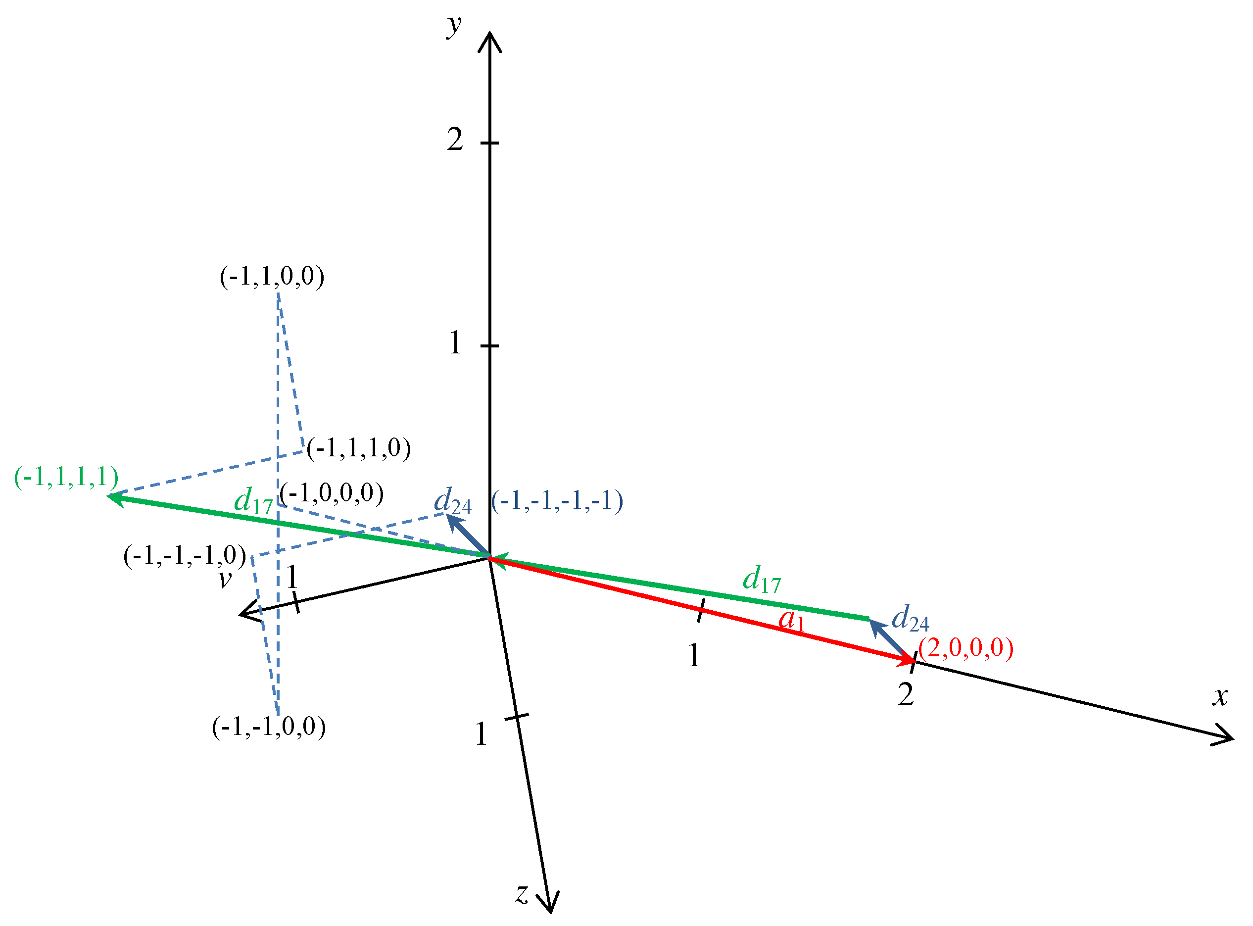
Although seems an algebraic object, it has strong geometric and optimization meanings. Matrix A has the property in any dimension that if a vector a (or d) is its column, then the vector (or ) is a column of A as well. For the first look, the elements of describe elementary circuits of the grid. For example, (see also Figure 1). Thus, starting from a point and making the steps of types 1, 17, and 24, the walk returns to the origin. However, there is another interpretation of the equation as follows:
implying that
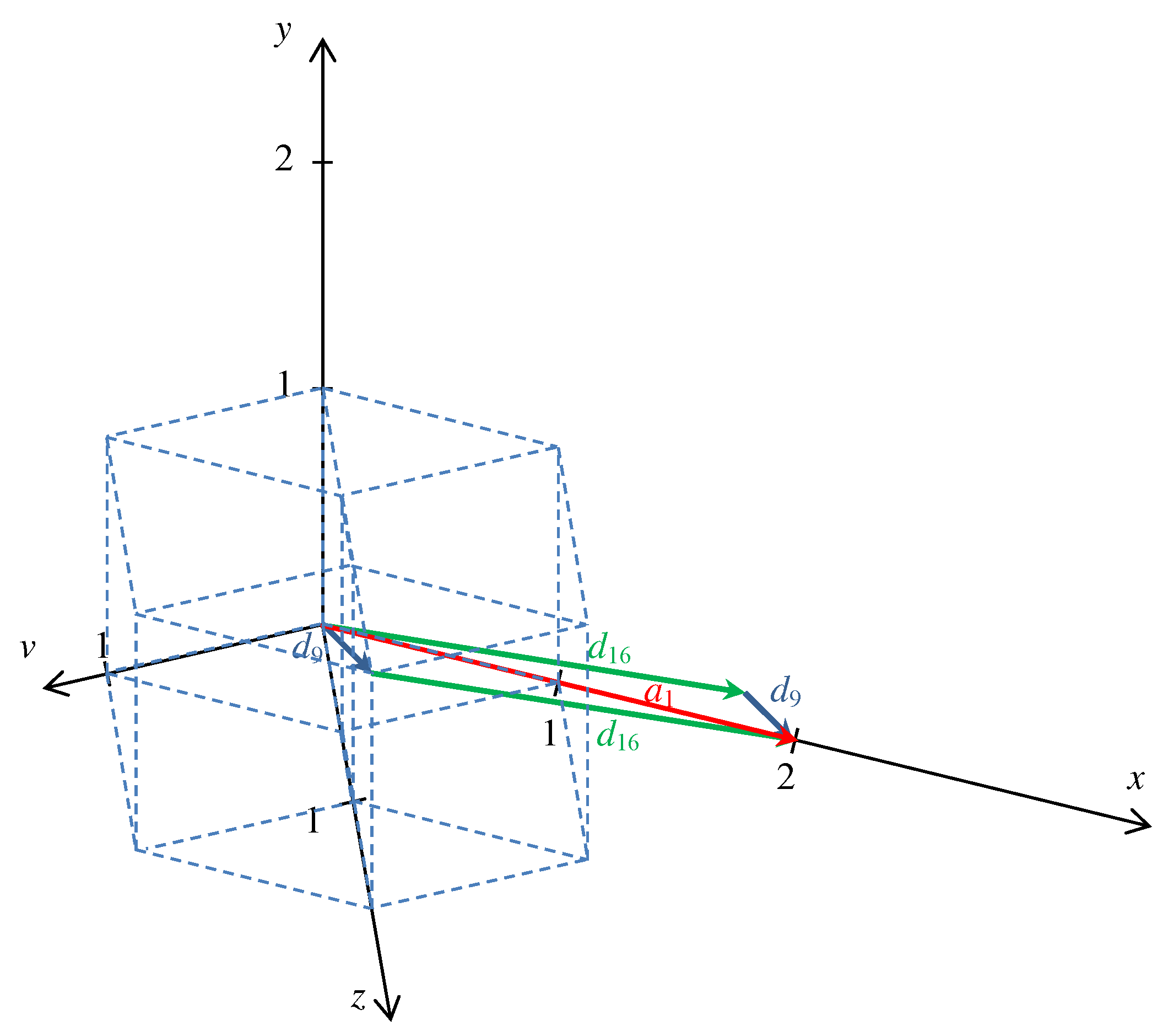
The meaning of the Equation (45) is that one step in the same rectangular sublattice is equivalent with two steps between the two sublattices (see also Figure 2). Thus, stepping in the same sublattice is better than the two steps between the sublattices if .
If the opposite inequality is true, i.e., , then it is better to step always between the sublattices. This example has further three similar cases as follows:
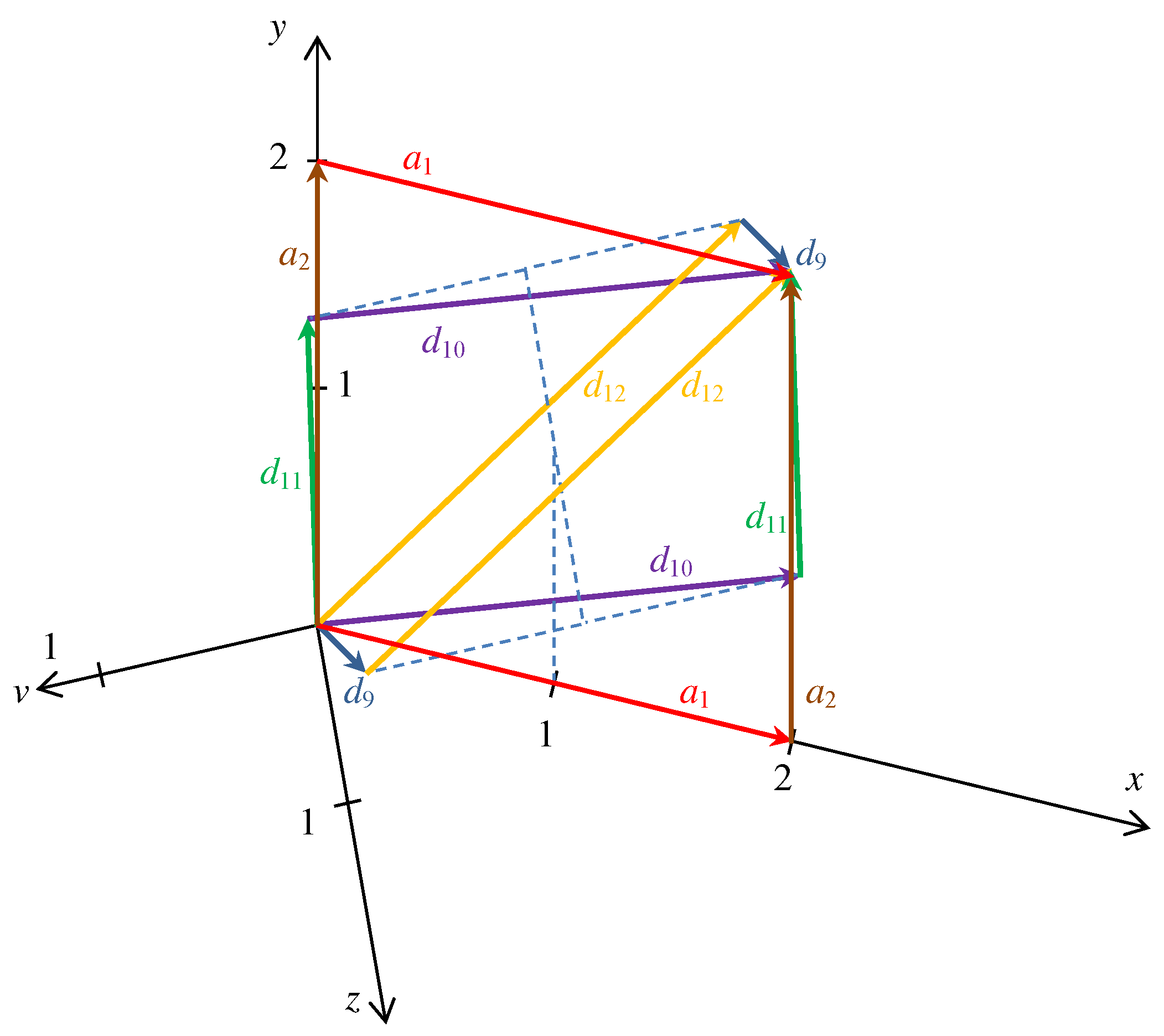
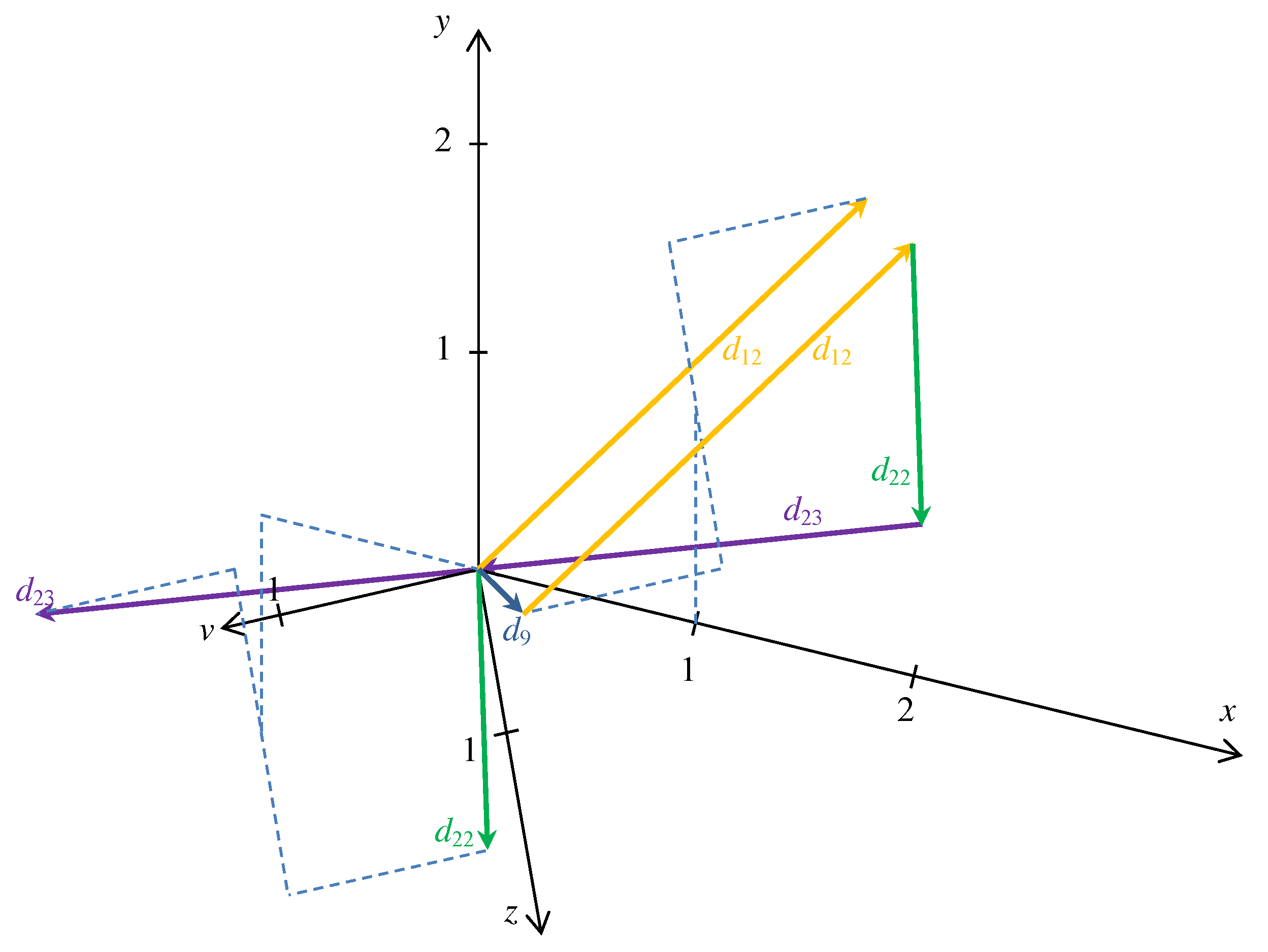
As we can see, a cycle in an undirected graph may have two different important interpretations as to walk a cycle arriving back to the initial point or to walk from a point to another in two different paths [21]. Many further composite steps can be obtained from Table 2. For example, it is possible to go from the origin to the point (2,2,0,0) by using steps and with length or with by using either steps and , or and as it is shown in Figure 3. A cycle form of the same relation based on the above-mentioned diagonal steps can be seen in Figure 4.
There is an iterative way to explore many elements of the Hilbert basis. The basic idea is that the known elements are excluded and the optimization problem looks for the next unknown element having the smallest norm. The model has variables , where the meaning of is that step j is used how many times in the circuit as in (42) or (43). Thus, it must be an integer. There is a second set of variables denoted by . They are binary variables as follows:
The meaning of is if the step represented by the jth column of matrix A is included in the circuit or not.
The objective function is the minimization of the number of used types of steps
Then the constraint being in the kernel space is similar to constraint (7) but the right-hand side must be the zero vector
The relation of the two types of variables is, that if if and only if . Let M be a big positive number. The constraint to be claimed is
Notice that (50) claims only that if is positive, then . However, it is not possible in an optimal solution that and . The zero vector must be excluded by claiming that the sum of the variables must be at least 1
The variables must be non-negative integer and binary, respectively,
The problems (48)–(52) are used in an iterative way. When a new member of the Hilbert basis is found, then it is excluded by the constraint that not all same types of steps can occur in a new element. Let be the last optimal solution. Lest . Then the inequality
is added to the problem as a new constraint. The next optimal solution must be different from .
Some trivially existing solution, i.e., if the sum of two columns is the zero vector, can be excluded immediately. Thus, the constraints
can be introduced.
The types obtained by iterative application of the model are summarized in Table 2.
A sequence of optimal bases of the linear relaxation is discussed in Theorem 3. The relation of the changes of the bases and the elements of the Hilbert basis is shown in Table 3. The relation can be obtained in the way shown in formula (44). Notice that the ratios of the numbers of a and d vectors are the same of the ratios of u and v where the optimal solution changes according to Theorem 2. The elements of the Hilbert basis can be obtained by taking the difference of the two optimal solutions.
It is easy to see from formula (37) that when the optimal fractional solution is converted to optimal integer solution, then a type 10 member of the Hilbert basis has a key role. It is .
9. Conclusions
This paper continues the analysis of the BCC grids started in [22]. It generalizes the grids to 4 and higher dimensions. Minimal routes are determined from the origin to a target point. An integer linear programming model is applied. Its linear programming relaxation is solved by the simplex method. There is only one case when the optimal solution is fractional. The integrality is achieved by the Gomory method in this case. In 4D, Table 1 shows the direct formulae to compute distance based on Theorem 2 (and generalized to nD in Corollary 1). The non-negative cone of the kernel space of the matrix of the steps in the grid has an important role. The elements of its Hilbert basis describe the alternative routes, i.e., the geometry of the routes, and the changes of the bases during the simplex method.
Author Contributions
Formal analysis, G.K., G.S. and N.D.T.; visualization, B.N.; writing—original draft preparation, B.V.; writing–review and editing, G.K. and B.N. All authors have read and agreed to the published version of the manuscript.
Funding
This research received no external funding.
Conflicts of Interest
The authors declare no conflict of interest.
Appendix A

Table A1.
The bases remained after the filtering of the 4-dimensional case containing no vectors from the first 8 vectors, i.e., containing only diagonal vectors. (The columns of matrix A are referred by their indices from 1 to 24).
Table A1.
The bases remained after the filtering of the 4-dimensional case containing no vectors from the first 8 vectors, i.e., containing only diagonal vectors. (The columns of matrix A are referred by their indices from 1 to 24).
| No. | Basis | Optimal | No. | Basis | Optimal | ||||||
|---|---|---|---|---|---|---|---|---|---|---|---|
| 1 | 9 | 10 | 11 | 13 | YES | 2 | 9 | 10 | 11 | 14 | YES |
| 3 | 9 | 10 | 11 | 15 | YES | 4 | 9 | 10 | 11 | 16 | YES |
| 5 | 9 | 10 | 12 | 13 | YES | 6 | 9 | 10 | 12 | 14 | YES |
| 7 | 9 | 10 | 12 | 15 | YES | 8 | 9 | 10 | 12 | 16 | YES |
| 9 | 9 | 10 | 15 | 19 | NO | 10 | 9 | 10 | 15 | 20 | NO |
| 11 | 9 | 10 | 16 | 19 | NO | 12 | 9 | 10 | 16 | 20 | NO |
| 13 | 9 | 11 | 12 | 14 | YES | 14 | 9 | 11 | 14 | 18 | NO |
| 15 | 9 | 11 | 14 | 20 | NO | 16 | 9 | 11 | 16 | 18 | NO |
| 17 | 9 | 12 | 13 | 14 | YES | 18 | 9 | 12 | 13 | 18 | NO |
| 19 | 9 | 12 | 13 | 22 | NO | 20 | 9 | 12 | 14 | 15 | YES |
| 21 | 9 | 12 | 14 | 16 | YES | 22 | 9 | 12 | 14 | 17 | NO |
| 23 | 9 | 12 | 14 | 18 | NO | 24 | 9 | 12 | 14 | 20 | NO |
| 25 | 9 | 12 | 14 | 22 | NO | 26 | 9 | 12 | 14 | 23 | NO |
| 27 | 9 | 12 | 15 | 22 | NO | 28 | 9 | 12 | 16 | 18 | NO |
| 29 | 9 | 12 | 16 | 22 | NO | 30 | 9 | 14 | 15 | 20 | NO |
| 31 | 9 | 14 | 16 | 20 | NO | 32 | 9 | 16 | 18 | 19 | NO |
| 33 | 9 | 16 | 18 | 20 | NO | 34 | 9 | 16 | 20 | 22 | NO |
| 35 | 10 | 11 | 12 | 13 | YES | 36 | 10 | 11 | 13 | 14 | YES |
| 37 | 10 | 11 | 13 | 15 | YES | 38 | 10 | 11 | 13 | 16 | YES |
| 39 | 10 | 11 | 13 | 17 | NO | 40 | 10 | 11 | 13 | 18 | NO |
| 41 | 10 | 11 | 13 | 19 | NO | 42 | 10 | 11 | 13 | 21 | NO |
| 43 | 10 | 11 | 13 | 24 | NO | 44 | 10 | 11 | 14 | 17 | NO |
| 45 | 10 | 11 | 14 | 21 | NO | 46 | 10 | 11 | 15 | 17 | NO |
| 47 | 10 | 11 | 15 | 21 | NO | 48 | 10 | 11 | 16 | 21 | NO |
| 49 | 10 | 12 | 13 | 17 | NO | 50 | 10 | 12 | 13 | 19 | NO |
| 51 | 10 | 12 | 15 | 17 | NO | 52 | 10 | 13 | 15 | 19 | NO |
| 53 | 10 | 13 | 16 | 19 | NO | 54 | 10 | 15 | 17 | 19 | NO |
| 55 | 10 | 15 | 17 | 20 | NO | 56 | 10 | 15 | 19 | 21 | NO |
| 57 | 11 | 12 | 13 | 18 | NO | 58 | 11 | 12 | 14 | 17 | NO |
| 59 | 11 | 13 | 14 | 18 | NO | 60 | 11 | 13 | 16 | 18 | NO |
| 61 | 11 | 14 | 17 | 18 | NO | 62 | 11 | 14 | 17 | 20 | NO |
| 63 | 11 | 14 | 17 | 21 | NO | 64 | 12 | 13 | 14 | 17 | NO |
| 65 | 12 | 13 | 17 | 18 | NO | 66 | 12 | 13 | 17 | 22 | NO |
| 67 | 12 | 13 | 18 | 19 | NO | 68 | 12 | 14 | 15 | 17 | NO |
References
- Klette, R.; Rosenfeld, A. Digital Geometry—Geometric Methods for Digital Picture Analysis; Morgan Kaufmann, Elsevier Science B.V.: Amsterdam, The Netherlands, 2004. [Google Scholar]
- Rosenfeld, A.; Pfaltz, J.L. Distance functions on digital pictures. Pattern Recognit. 1968, 1, 33–61. [Google Scholar] [CrossRef]
- Borgefors, G. Distance transformations in digital images. Comput. Vision Graph. Image Process. 1986, 34, 344–371. [Google Scholar] [CrossRef]
- Csébfalvi, B. Prefiltered Gaussian Reconstruction for High-Quality Rendering of Volumetric Data sampled on a Body-Centered Cubic Grid. In Proceedings of the VIS 05—IEEE Visualization 2005, Minneapolis, MN, USA, 23–28 October 2005; pp. 311–318. [Google Scholar]
- Csébfalvi, B. An Evaluation of Prefiltered B-Spline Reconstruction for Quasi-Interpolation on the Body-Centered Cubic Lattice. IEEE Trans. Vis. Comput. Graph. 2010, 16, 499–512. [Google Scholar] [CrossRef] [PubMed]
- Vad, V.; Csébfalvi, B.; Rautek, P.; Gröller, M.E. Towards an Unbiased Comparison of CC, BCC, and FCC Lattices in Terms of Prealiasing. Comput. Graph. Forum 2014, 33, 81–90. [Google Scholar] [CrossRef]
- Strand, R.; Nagy, B. Path-Based Distance Functions in n-Dimensional Generalizations of the Face- and Body-Centered Cubic Grids. Discret. Appl. Math. 2009, 157, 3386–3400. [Google Scholar] [CrossRef] [Green Version]
- Kovács, G.; Nagy, B.; Vizvári, B. Weighted Distances and Digital Disks on the Khalimsky Grid—Disks with Holes and Islands. J. Math. Imaging Vis. 2017, 59, 2–22. [Google Scholar] [CrossRef]
- Remy, E.; Thiel, E. Computing 3D Medial Axis for Chamfer Distances. In Proceedings of the DGCI 2000: Discrete Geometry for Computer Imagery—9th International Conference, Lecture Notes in Computer Science, Uppsala, Sweden, 13–15 December 2000; Volume 1953, pp. 418–430. [Google Scholar]
- Sintorn, I.-M.; Borgefors, G. Weighted distance transforms in rectangular grids. In Proceedings of the ICIAP, Palermo, Italy, 26–28 September 2001; pp. 322–326. [Google Scholar]
- Butt, M.A.; Maragos, P. Optimum design of chamfer distance transforms. IEEE Trans. Image Process. 1998, 7, 1477–1484. [Google Scholar] [CrossRef] [PubMed]
- Celebi, M.E.; Celiker, F.; Kingravi, H.A. On Euclidean norm approximations. Pattern Recognit. 2011, 44, 278–283. [Google Scholar] [CrossRef] [Green Version]
- Kovács, G.; Nagy, B.; Vizvári, B. On disks of the triangular grid: An application of optimization theory in discrete geometry. Discret. Appl. Math. 2020, 282, 136–151. [Google Scholar] [CrossRef]
- Kovács, G.; Nagy, B.; Vizvári, B. Chamfer distances on the isometric grid: A structural description of minimal distances based on linear programming approach. J. Comb. Optim. 2019, 38, 867–886. [Google Scholar] [CrossRef]
- Ahuja, R.K.; Magnanti, T.L.; Orlin, J.B. Network Flows: Theory, Algorithms and Applications; Prentice Hall: Upper Saddle River, NJ, USA, 1993. [Google Scholar]
- Dantzig, G.B. Programming in a Linear Structure, Report of the September 9, 1948 meeting in Madison. Econometrica 1949, 17, 73–74. [Google Scholar]
- Prékopa, A. Lineáris Programozás I; Hungarian, Linear Programming I; Bolyai János Matematikai Társulat (János Bolyai Mathematical Society): Budapest, Hungary, 1968. [Google Scholar]
- Hilbert, D. Über die Theorie der algebrischen Formen. Math. Ann. 1890, 36, 473–534. [Google Scholar] [CrossRef]
- Jeroslow, R.G. Some basis theorems for integral monoids. Math. Oper. Res. 1978, 3, 145–154. [Google Scholar]
- Schrijver, A. On total dual integrality. Linear Algebra Its Appl. 1981, 38, 27–32. [Google Scholar] [CrossRef] [Green Version]
- Nagy, B. Union-Freeness, Deterministic Union-Freeness and Union-Complexity. In Proceedings of the DCFS 2019: Descriptional Complexity of Formal Systems—21st IFIP WG 1.02, International Conference, Lecture Notes in Computer Science, Kosice, Slovakia, 17–19 July 2019; Volume 111612, pp. 46–56. [Google Scholar]
- Kovács, G.; Nagy, B.; Stomfai, G.; Turgay, N.D.; Vizvári, B. On Chamfer Distances on the Square and Body-Centered Cubic Grids—An Operational Research Approach. 2021; Unpublished work. [Google Scholar]
Figure 1.
The sum of vectors , , and is the four-dimensional zero vector. The coordinates of the construction are also shown.
Figure 1.
The sum of vectors , , and is the four-dimensional zero vector. The coordinates of the construction are also shown.

Figure 2.
The sum of vectors and is exactly the vector in the four-dimensional BCC grid. A unit hypercube is also shown.
Figure 2.
The sum of vectors and is exactly the vector in the four-dimensional BCC grid. A unit hypercube is also shown.

Figure 3.
Alternative paths from to , each is built up by two steps, in the four-dimensional BCC grid.
Figure 3.
Alternative paths from to , each is built up by two steps, in the four-dimensional BCC grid.

Figure 4.
The sum of four diagonal vectors is the zero vector, each vector is also shown from the origin.
Figure 4.
The sum of four diagonal vectors is the zero vector, each vector is also shown from the origin.

Table 1.
The optimal solutions, i.e., distances between and .
| Basis | Variables | The Value of the Objective Function | Optimality Condition |
|---|---|---|---|
| , , , | |||
| , , , | |||
| , , , | |||
| , , , | |||
| , , , |
Table 2.
Types of the elements of the Hilbert basis.
| Type | # of a’s | # of d’s | Example | # of Cases |
|---|---|---|---|---|
| 1 | 2 | 0 | 4 | |
| 2 | 0 | 2 | 8 | |
| 3 | 1 | 2 | 32 | |
| 4 | 2 | 2 | 48 | |
| 5 | 0 | 4 | 24 | |
| 6 | 3 | 2 | 32 | |
| 7 | 1 | 4 | 64 | |
| 8 | 0 | 6 | 16 | |
| 9 | 2 | 4 | 16 | |
| 10 | 4 | 2 | 16 |
Table 3.
The relation of the elements of the Hilbert basis and the changes of basis.
| Old Basis | New Basis | Hilbert Basis Element | Type | Ratio |
|---|---|---|---|---|
| 10 | ||||
| 6 | ||||
| 4 | ||||
| 3 |
Publisher’s Note: MDPI stays neutral with regard to jurisdictional claims in published maps and institutional affiliations. |
© 2021 by the authors. Licensee MDPI, Basel, Switzerland. This article is an open access article distributed under the terms and conditions of the Creative Commons Attribution (CC BY) license (http://creativecommons.org/licenses/by/4.0/).
Share and Cite
MDPI and ACS Style
Kovács, G.; Nagy, B.; Stomfai, G.; Turgay, N.D.; Vizvári, B. Discrete Optimization: The Case of Generalized BCC Lattice. Mathematics 2021, 9, 208. https://doi.org/10.3390/math9030208
AMA Style
Kovács G, Nagy B, Stomfai G, Turgay ND, Vizvári B. Discrete Optimization: The Case of Generalized BCC Lattice. Mathematics. 2021; 9(3):208. https://doi.org/10.3390/math9030208
Chicago/Turabian StyleKovács, Gergely, Benedek Nagy, Gergely Stomfai, Neşet Deniz Turgay, and Béla Vizvári. 2021. "Discrete Optimization: The Case of Generalized BCC Lattice" Mathematics 9, no. 3: 208. https://doi.org/10.3390/math9030208
Note that from the first issue of 2016, this journal uses article numbers instead of page numbers. See further details here.