Particulate Matter Profiles along the Rack Railway Route Using Low-Cost Sensor

Abstract

Air pollution due to Particulate Matter (PM) is an increasing concern of global extent. It has been the focus of many research projects worldwide and the latest low-cost technology is offering an ease and cheap way to monitor PM concentration. In this research, a low-cost PM monitoring platform was built with the objectives of evaluating its feasibility and its performance in mobile measurements, as well as characterizing the concentration profiles of PM along the measurement route. The rack railway in Stuttgart was utilized as means of transportation for this low-cost monitoring system with which the temporal and spatial distribution of the PM10, PM2.5 and PM1 concentration along the route was attained. The measurements were conducted for around two months from mid of January until mid of March 2019, during the operation hours of the rack railway. The results showed that the PM concentrations were dominated by fine particulate matter (PM2.5 and PM1) along the route of the rack railway. Higher PM concentrations were measured near the federal highway and high traffic area as compared to the residential area. An overestimation of PM concentration using low-cost sensor platform was observed during high relative humidity conditions as compared to the professional aerosol spectrometers.

1. Introduction

Air pollution is a serious health concern. It is one of the major environmental challenges across the globe. Constant population growth, continuous increases in energy and food demand, rapid human activities such as urbanization and deforestation intensify this issue [1,2,3,4]. According to the World Health Organization (WHO), ambient air pollution increased globally by 8% between 2008 and 2013 [5] while around 7 million deaths worldwide every year are due to exposure from household and outdoor air pollution [6]. One of the main pollutants in ambient air is particulate matter (PM), especially in urbanized areas. Several studies linked the increase in ambient PM exposure to a range of different respiratory health diseases such as lung cancer, asthma and Chronic Obstructive Pulmonary Disease (COPD) [7,8,9].

Mobile measurements help to measure the air quality in an extended area and provide a high spatial resolution of the measured parameters. These measurements enhance the information obtained from a network of stationary monitoring stations, which are often influenced by near emission sources, at least when situated in urban hotspot areas, and represent mostly the local surrounding conditions [10]. Different means of transportation can be used to perform mobile measurements, for instance, a measurement car [11] or a bicycle [12] or even walking on foot [13]. The public transportation system was also used as a platform for mobile measurements of ambient air quality [10].

Generally, low-cost PM sensors provide the means for mobile measurements, due to their compact form, lightweight and low costs. These low-cost sensors rely mostly on well-researched principles, such as the light scattering of particles [14,15]. Low-cost sensors allow higher spatial coverage compared to the current reference methods for air pollutant measurements and can decrease the need for skilled operators for maintenance and calibration of monitoring devices [16]. Nevertheless, some disadvantages of these sensors are the questionable quality of the raw data, reliability of the results and the influence of meteorological parameters on the measured results [17]. The low-cost PM sensors are known to overestimate the measured PM concentration during high humidity or foggy conditions [18,19,20].

For this study, the rack railway in Stuttgart was selected to carry out mobile measurements in a semi-automated manner. The rack railway is a city tram that uses a toothed rack rail between the running rail. This is necessary due to the steepness of the slope. It is one of the last four of its kind in Germany and the only one, which is fully integrated into the public transportation system [21]. The route passes not only through traffic-exposed areas such as the federal highway B27, but also through traffic-free areas like pedestrian precincts and near private backyards. In order to measure the temporal and spatial distribution of PM in the ambient air, a low-cost PM monitoring platform was built. This platform contained a low-cost PM sensor, sensors to measure temperature, relative humidity and pressure with respective electronic parts. A GPS was also included to determine the geographical position.

2. Measurement Technique and Methodology

2.1. Measurement Location and Duration

This study was conducted in the city of Stuttgart in Germany, which is well known due to its air quality problems. It is the sixth largest city in Germany with around 630,000 inhabitants [22]. Stuttgart is located in a valley surrounded by hills from three sides and possesses a complex topography, which has a significant influence on climatic elements like radiation, temperature, humidity and wind [23]. Stuttgart is a great example of low wind speeds in the southern part of Germany, due to mountain ranges and the distance from the sea, which limit the air exchange and dilution of pollutants. In addition, the precipitation is low with approx. 600 mm per year due to the lee effects of the mountains, leading to little wet deposition. Both factors inhibit air exchange and are therefore important meteorological reasons for high concentrations of air pollutants in Stuttgart [24]. The traffic in Stuttgart also plays an important role in the air quality of the city. It is considered as the main emission source for air pollution in the city [25]. The lack of ring roads around the city, leads to most of the traffic passing through the city [26]. High traffic loads lead to high emissions of nitrogen oxides, PM and UFP from the vehicle exhaust as well as PM from the abrasion of brakes, tires, asphalt and clutches [27].

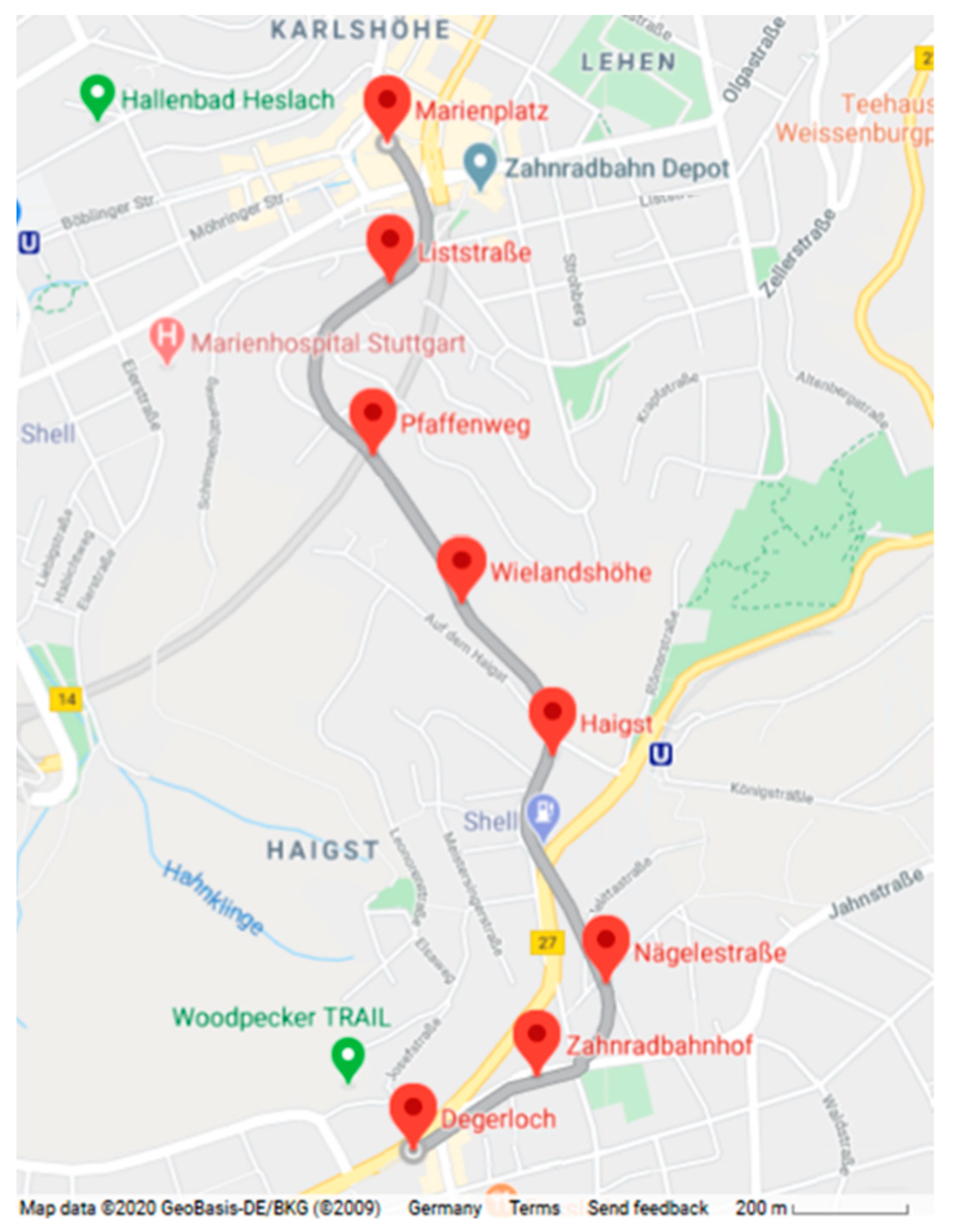
The rack railway is considered as a vital part of the city’s transportation system and to reach the objectives of this measurement campaign. The route of the rack railway starts at the “downtown station” Marienplatz, which is located in the south of Stuttgart’s city center and ends uphill at the “hill station” called Degerloch, as shown in Figure 1. Red pins indicate the stations on the route. The route is around 2.2 km long, which is surrounded by street intersections, green-residential areas and two busy highways (Federal highway B14 and B27). The number of vehicles using the two federal highways B14 and B27 reaches around 150,000 vehicles per day [23]. The altitude of the route increases when moving from Marienplatz to Degerloch. It starts at 262 m a.s.l. (above sea level) at Marienplatz, then 353 m a.s.l. at Pfaffenweg, 431 m a.s.l. at Haigst until it reaches 470 m a.s.l. at Degerloch. This elevation difference provides the possibility for capturing a vertical profile of the meteorological parameters and air pollutants as well as a certain horizontal profile. It could potentially help in examining the influence of inversion on PM profiles.

The measurement campaign started in winter from mid of January 2019 until mid of March 2019. During this period, the measurements were performed for around 1600 trips in total with an average of 27 trips per day. The operation hours for the rack railway during this period were from 5:00 a.m. until 8:55 p.m. on the working days (Monday–Saturday) and from 6:30 a.m. until 8:55 p.m. on Sundays and on holidays. One trip from Marienplatz to Degerloch and back took 30 min in total with a travelling time of 20 min and a waiting time of 10 min. The rack railway moves with an average speed of around 20 km/h, requiring 10 min to travel from Marienplatz to Degerloch. There it waited for four minutes for the passengers to board or leave the wagon. After that, it took 10 min to travel back from Degerloch to Marienplatz, where a six-minute stop was made.

2.2. Measurement Setup

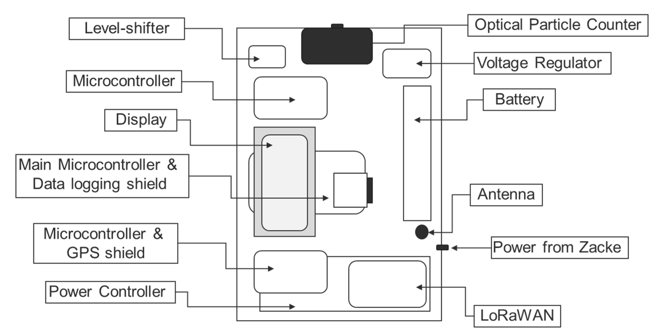
To measure PM concentrations along this route, a sensor-monitoring box was created. The box is an experimental low-cost PM monitoring platform designed and constructed at the Department of Air Quality Control at the University of Stuttgart in order to investigate PM concentrations. This multi-processor system was used for remotely measuring the outdoor PM concentrations. The sensor-monitoring box consists of three Arduino microcontrollers, which were working asynchronously with a GPS shield, a data-logging shield, a power controller and an Alphasense sensor (OPC-N2).

The Alphasense OPC-N2 sensor is a low-cost laser scattering PM sensor. It measures the light scattered by individual particles carried in a sample air stream through a laser beam. This low-cost PM sensor has a measurement size range from 0.38 μm to 17 μm sorting into 16 size bins. It provides a real-time histogram as well as the flowrate of the sampling air [28]. Two Arduino Uno microcontrollers control this sensor and the GPS shield. The GPS shield was an Adafruit Ultimate GPS Logger Shield, which includes a low-power GPS module and has a positional accuracy of 3 m. The main controller of this platform was an Arduino Mega, which carried the data logging shield. It collected the information from both Arduino Uno microcontrollers and stored them on a SD-card. In addition, it was responsible for monitoring the battery voltage, the current location of the box and the measured PM concentration on the attached LCD display. A Long Range Wide Area Network (LoRaWAN) was selected as remote communication system to help carrying out the autonomous out-door measurements. The LoRaWAN is one of the Low Power Wide Area Network (LPWAN) technologies that has received significant attention from the research community in recent years. It offers low-power, low-data rate communication over a wide range of covered areas [29]. Since the signal coming from the LoRaWAN is a wireless radio protocol, a transmitter was used to handle the wireless protocol. The main aim of using the LoRaWAN was to establish a remote communication to monitor the activation status of the box, battery voltage and working of the sensor-monitoring box. To run the system, the power was supplied from the rack railway. A voltage regulator was used before the power reached the power controller. Using a voltage regulator helped to save the electronics from any damage by alternating voltage and to provide the box with a stable voltage. The power controller was a custom-made circuit containing an Arduino MKR relay proto shield, switches, LED lights, a printed circuit board and other electronics. It was responsible for charging the battery and providing power to the microcontrollers. The general layout for all those components is shown in Figure 2.

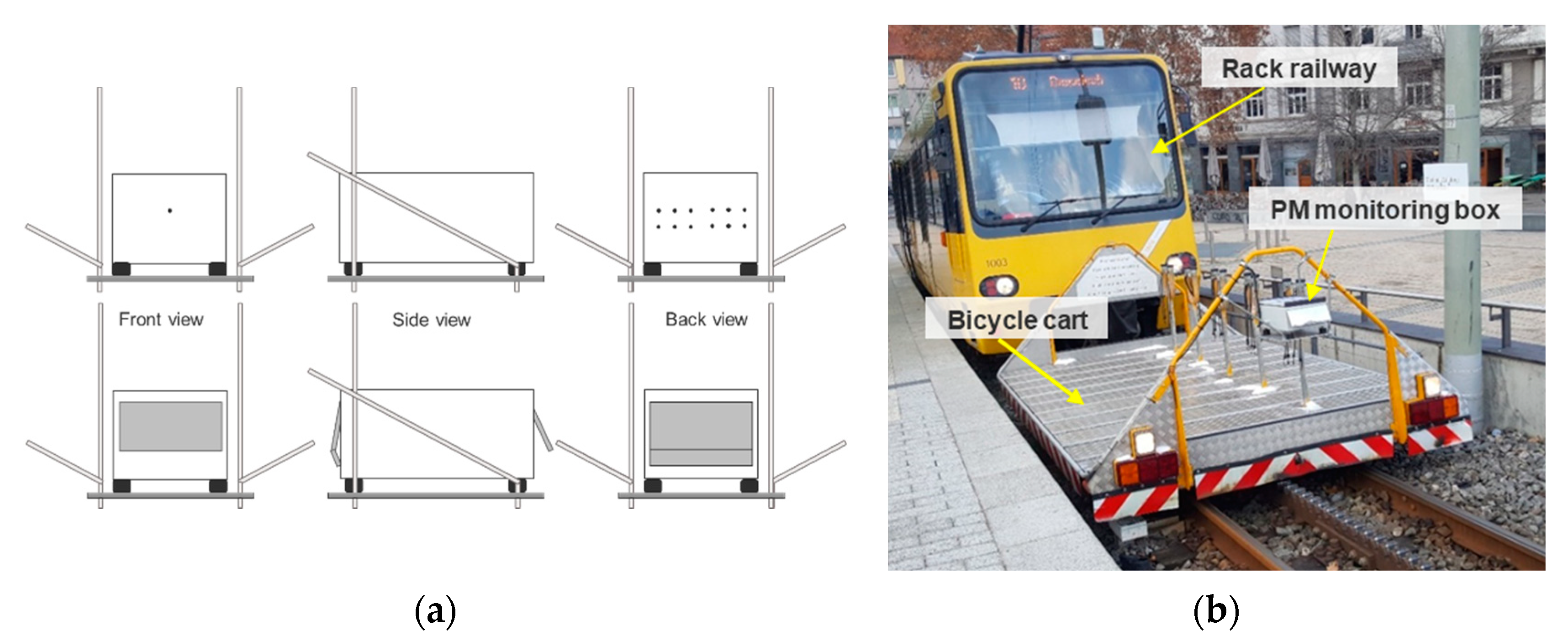
All of these components were installed inside a closed box in order to keep the electronics and the sensitive parts safe from damage, theft and harsh weather conditions. Additionally, a custom-made box hanger was built specifically to carry the box on the rack railway. It was mounted on the front of the bicycle cart of the rack railway with an inlet height of around 1 m from the ground. Figure 3 shows the mounting mechanism for the sensor-monitoring box and its mounting location on the bicycle cart of the rack railway. The custom-made box-hanger on which the box was mounted is shown in Figure 3a. The front, side and back view are displayed for a better understanding. The front and back of the box have holes for inlet and outlet respectively. The holes are covered with a metal sheet to avoid rain or water droplets destroying the platform. Figure 3a illustrates the box and hanger with and without the metal sheet. In Figure 3b the position of the sensor-monitoring box on the rack railway is shown.

The measured PM concentrations using the sensor-monitoring box were compared to two other PM monitoring devices, namely the stationary aerosol spectrometer Grimm EDM180 and the mobile aerosol spectrometer Grimm 1.108 from the company Grimm Aerosol Technik Ainring GmbH & Co. KG. Both these devices as well as the Alphasense OPC-N2 PM sensor work by the same detection principle, which is the light scattering principle [30,31]. The aerosol spectrometer Grimm 1.108 was used during certain trips to measure the PM concentrations along the route. It was directly mounted on top of the sensor-monitoring box in order to be subjected to the same measuring conditions. The setup is shown in Figure 4a. The aerosol spectrometer Grimm EDM180 was installed at the monitoring station at Marienplatz as shown in Figure 4b and measured continuously during the whole campaign. The data from this device was used for comparison with the concentrations measured using the sensor-monitoring box during the waiting time between the trips at Marienplatz. The time resolution of both the Grimm devices was six seconds while for the sensor-monitoring box it was five seconds. The Grimm EDM180 is a professional stationary aerosol spectrometer that has an inlet dryer while the Grimm 1.108 is a professional mobile aerosol spectrometer without any inlet dryer.

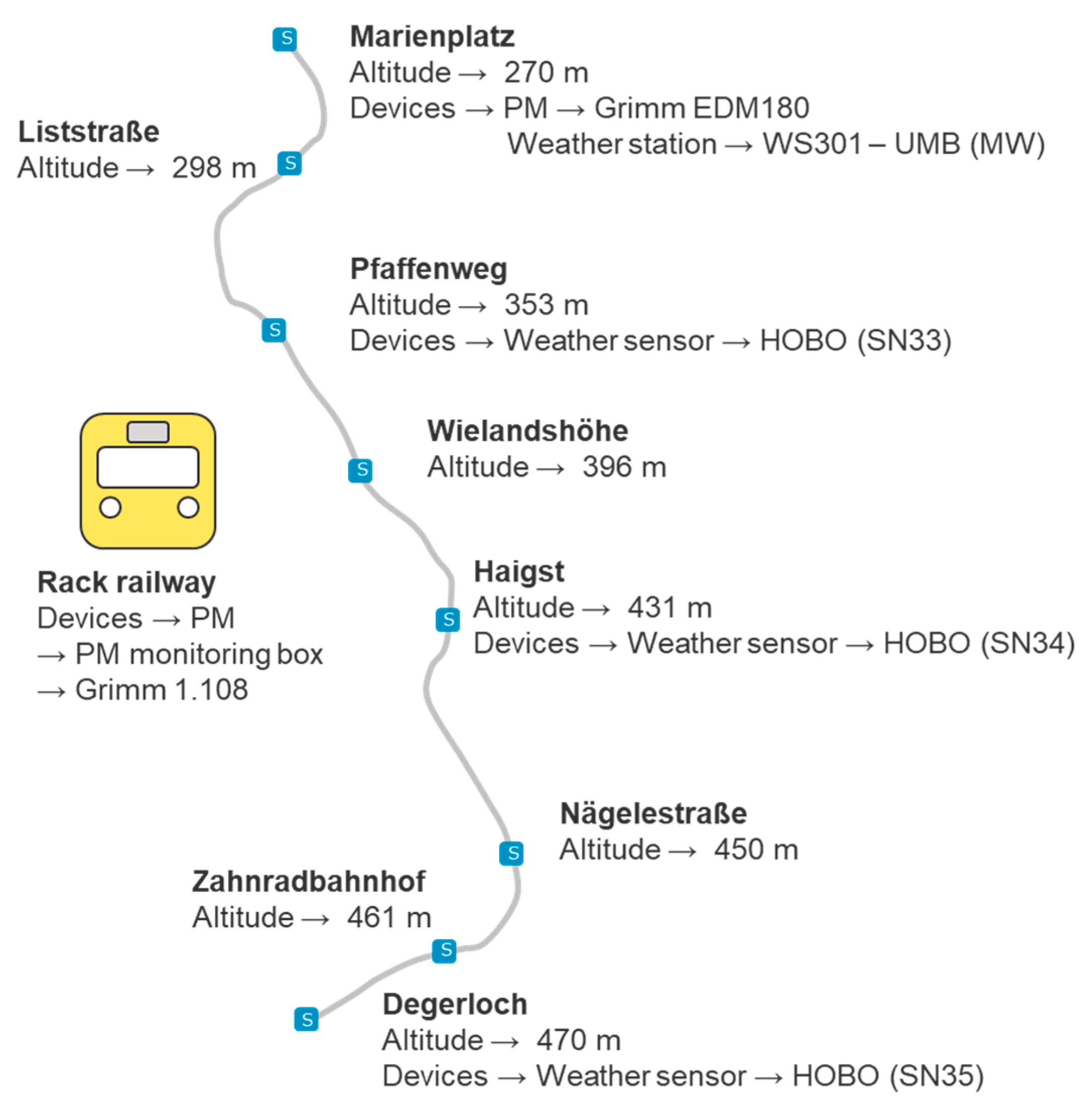
The relative humidity and air temperature were also measured during the measurement campaign. Monitoring the relative humidity and temperature assisted in better post-processing of the data. The compact weather sensor WS301-UMB of the company G. Lufft Mess- und Regeltechnik GmbH from the monitoring station at Marienplatz was used to represent the meteorological situation there. The WS301-UMB (MW) uses the Negative Temperature Coefficient (NTC) resistor principle to measure the temperature. In addition, it uses a capacitive humidity sensor to measure the relative humidity by the change of a capacitance [32]. Next to WS301-UMB (MW), three low-cost HOBO MX2302 sensors from the company Onset Computer Corporation were distributed along the route of the rack railway to measure the relative humidity and air temperature. The locations for these sensors were selected with the aim to achieve an approximate constant route coverage, i.e., regarding length and altitude. These low-cost sensors measure the meteorological conditions (relative humidity and air temperature), record the measured values on their internal memory and send this information via wireless connection with a mobile device [33]. Figure 5 shows the distribution of HOBO sensors along the route of the rack railway during the measurement campaign.

2.3. Data Analysis and Processing

Around 1600 trips were performed during the measurement campaign. The sensor-monitoring box measured PM10, PM2.5 and PM1 concentrations along the route during each trip. The time schedule of the rack railway and the stored GPS coordinates were consulted to allocate the measured PM concentrations using the sensor-monitoring box. Each trip was evaluated and plotted individually based on their time schedule using ArcGIS software from the company Esri Deutschland GmbH. The whole route was divided into segments of 20 m length, each of which is depicted by one circle indicating the average value of this segment in the maps.

The measured trips were not only dependent upon the operational hours but also on the direction of travel of the rack railway. During the first half of a trip, i.e., from Marienplatz to Degerloch, the inlet of the sensor-monitoring box was facing the direction of travel. However, that case was opposite during the second half of the trip, when the rack railway drove from Degerloch back to Marienplatz. The inlet of the sensor-monitoring box was behind the train. The suspected turbulence and the associated whirling up of fine particles can explain the increased concentrations that were found during the descent from Degerloch to Marienplatz. The data of the return trip, when the sensor-monitoring box was at the rear of the train, were discarded and not considered for the evaluation. ArcGIS software was also used to plot the PM concentrations measured using the mobile aerosol spectrometer Grimm 1.108.

3. Results and Discussion

3.1. PM Profiles along the Rack Railway Route

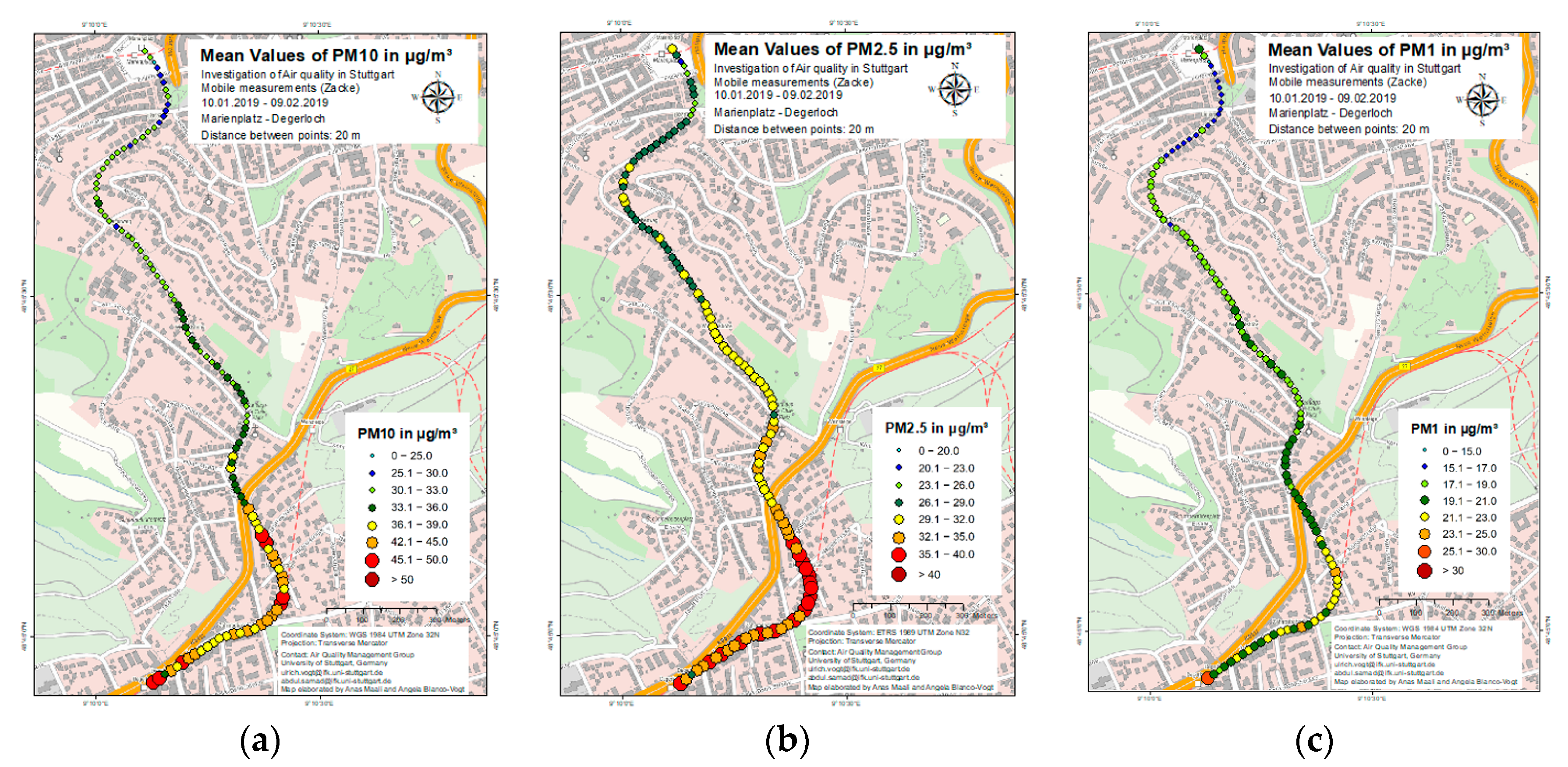
The PM profiles along the rack railway route were obtained during the measurement campaign. The results of these measurement profiles as an average for a period of one month from 10 January until 9 February 2019 are shown in Figure 6a–c for PM10, PM2.5 and PM1 respectively. These average PM concentration profiles display the typical PM concentration along the measurement route. For each trip, an information box, located at the top right of the figure shows the measured parameter, the distance for each segment, the starting and ending time, date and direction of the trip. For each measured parameter, a legend is located at the bottom right of the figure. As can be seen in Figure 6a for the concentration profile of PM10, the PM10 concentration at Marienplatz was relatively lower i.e., in the range of 25 to 30 µg/m³. Along the route, the PM10 concentration was around 30 µg/m³ in the residential area with less traffic. After approximately half of the route, the PM10 concentration started to increase and reached a concentration of more than 40 µg/m³ close to the federal highway B27. The PM10 concentration remained between 40 to 50 µg/m³ in Degerloch, where the maximum traffic along the measurement route was observed. Hence, the increase in PM10 concentration close to the federal highway B27 can be attributed to traffic as it is the main source of PM emission locally. The results of PM2.5 and PM1 shown in Figure 6b,c respectively, depict the same observation as for PM10. The PM2.5 concentrations at the start were around 25 µg/m³ while near the federal highway they increased to around 35 µg/m³. For PM1, the concentrations at the start and near the federal highway were around 15 µg/m³ and 20 µg/m³ respectively.

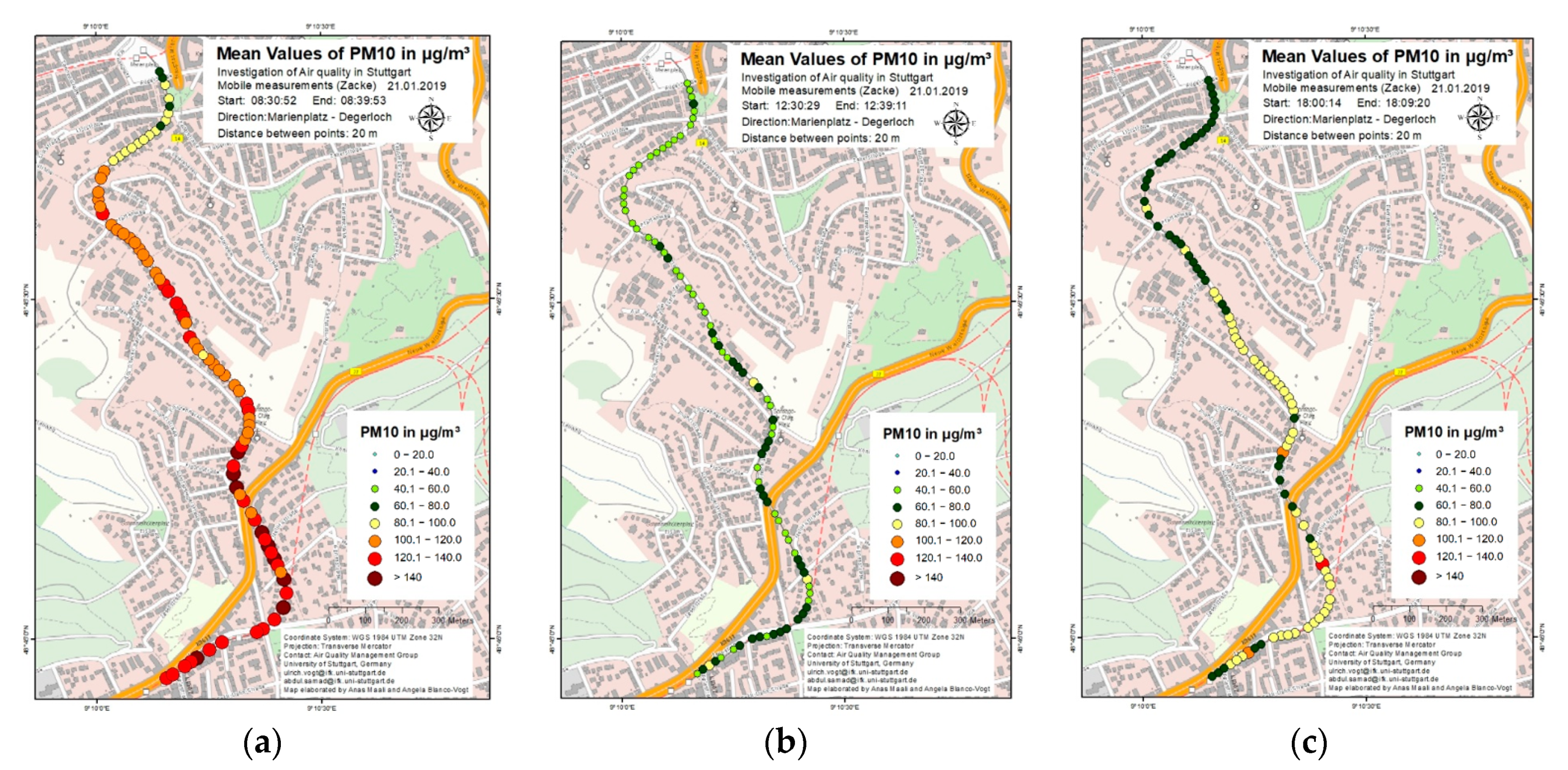
The average trips provide a general overview of the PM profiles along the measurement route. However, the individual trips provided information about the behavior of PM concentration in the investigated area at different times of the day. During the measurement campaign, intensive measurements were performed on some days in which the mobile aerosol spectrometer Grimm 1.108 was also used to compare the results obtained from the sensor-monitoring box. One such intensive measurement period was on 21 January 2019 and 22 January 2019. Figure 7a–c shows the measured PM10 concentration during three different trips on 21 January 2019 at morning, afternoon and evening, respectively. It can be seen in Figure 7a that very high PM10 concentrations of around 100 µg/m³ and above were measured during nearly the whole trip. No significant difference was observed between the residential and traffic areas. The PM10 concentration during the afternoon (Figure 7b) was the lowest compared to the trips in the morning and the evening that can be seen in Figure 7a,c. The PM10 concentration varied between 40 to 80 µg/m³ during this whole trip. Relatively lower PM10 concentrations were measured during the first half of the trip as compared to the higher PM10 concentration in the second half of the trip, which followed the general trend of the PM concentration profile along the measurement route, which could already be observed in Figure 6. The trip during the evening, presented in Figure 7c showed a slight increase in PM10 concentration as compared to the trip during the afternoon. This increase in concentration can be attributed to the high traffic during peak hours as well as more stable weather conditions in the evening compared to the afternoon, in wintertime.

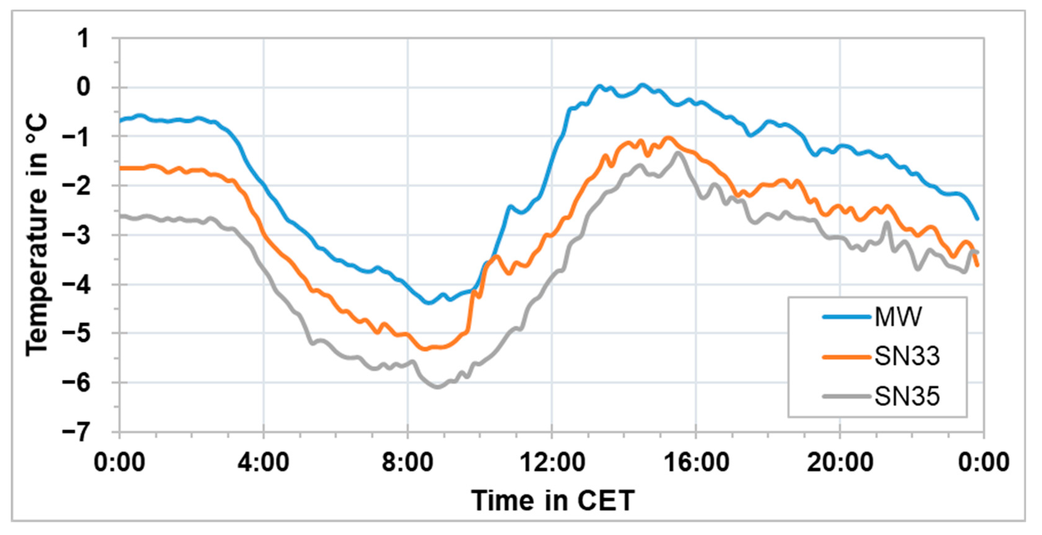
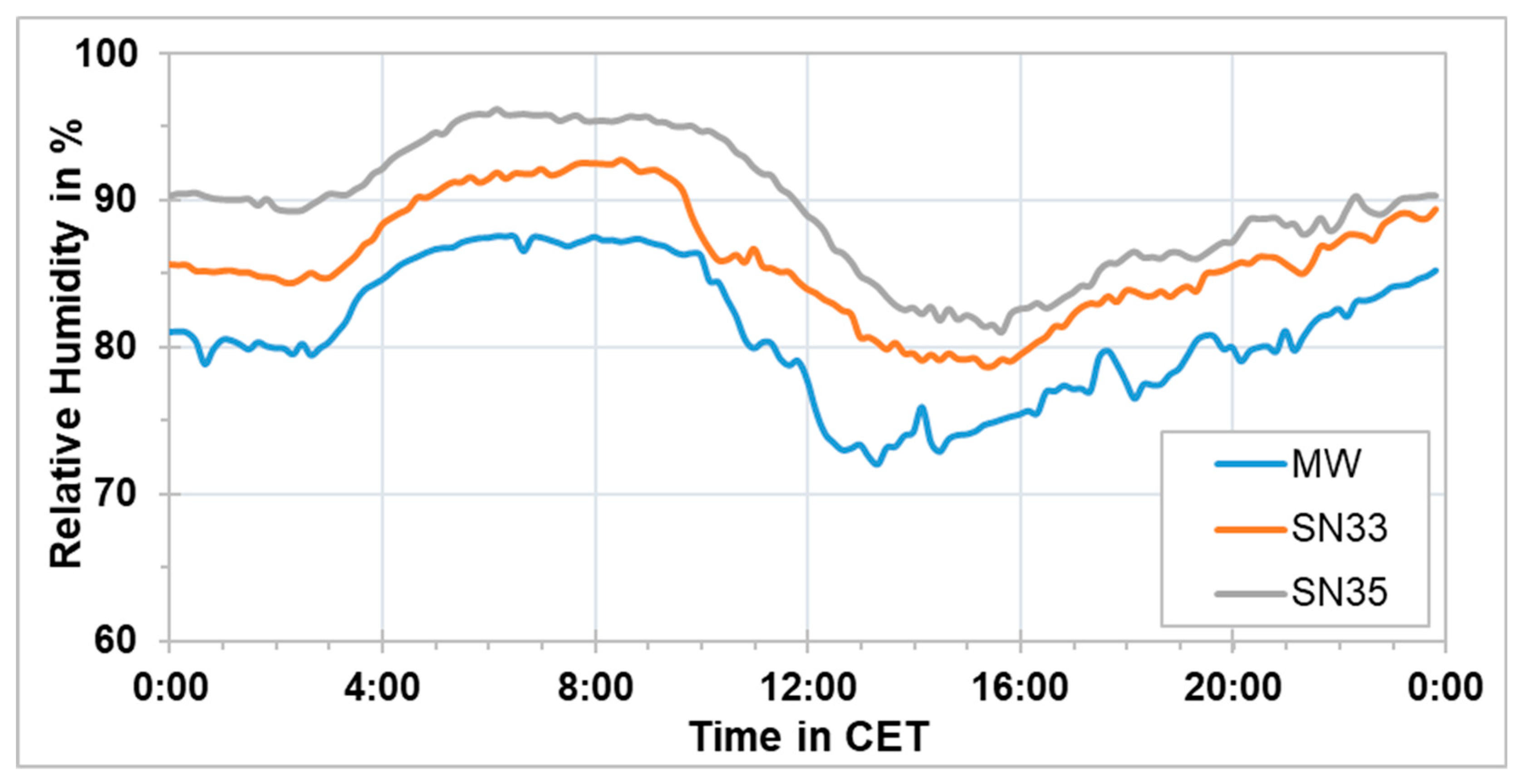
Possible reasons for the increased PM10 concentrations during the morning time were considered during the investigation. Since it was known from previous studies, as discussed in the introduction, that the low-cost PM sensors overestimate the concentration during foggy or high relative humidity conditions, the temperature and relative humidity along the measurement route were examined. The temperature and relative humidity were measured using the HOBO sensors (SN33, SN34, and SN35) and the compact weather sensor (MW). Generally, the measured temperatures during this measurement campaign were relatively low and the relative humidity levels were high. A common pattern of relative humidity and temperature along the route during the measurement campaign was observed. High relative humidity levels were noticed after midnight until around 9:00 CET. Between 9:00 CET–15:00 CET, the levels declined to the lowest values throughout the day. After 15:00 CET, the relative humidity values started to increase again. Those time intervals defined also the general temperature pattern along the route. Low temperatures were measured after midnight until around 9:00 CET. The temperature increased between 9:00 CET–15:00 CET after which it started to decrease again.

Figure 8 shows the measured air temperatures in °C and Figure 9 the relative humidity in percentage for the route on 21 January 2019. The data from SN34 was not available on that day due to some technical inadequacy. Low temperatures between −7 °C and 1 °C were observed along the route of the rack railway during this day. In addition, a clear temperature difference between the three locations was detected, i.e., Marienplatz (MW), Pfaffenweg (SN33) and Degerloch (SN35). During most trips, the lowest temperature was observed in Degerloch followed by Pfaffenweg and then Marienplatz. The estimated difference was around 2 °C between Marienplatz and Degerloch. An evident increase of the temperature was recorded from 9:00 CET–15:00 CET, which was around 4 °C. This increment resulted from the absorption of heat radiation of the sun by the surfaces and the transmission of energy from the heated surfaces to the nearby ground air masses during the day.

High relative humidity levels ranging between 70% and 95% were recorded on that day, with the relative humidity increasing with altitude. Around 10% difference in relative humidity levels was seen between Marienplatz (MW) and Degerloch (SN35). It was assumed that the high levels of relative humidity during the morning led to an overestimation of the measured PM10 concentrations using the sensor-monitoring box. However, more investigation is needed to prove this assumption.

3.2. PM Concentration Comparison between Sensor-Monitoring Box and Professional Aerosol Spectrometer

The rack railway stops for around six minutes at Marienplatz before starting each trip. During this stationary period, the sensor-monitoring box measured the PM concentration for the surrounding area, i.e., Marienplatz. The results shown in this section are a comparison between the measured concentrations using the sensor-monitoring box and the professional aerosol spectrometer Grimm EDM180, which was installed in the monitoring station at Marienplatz.

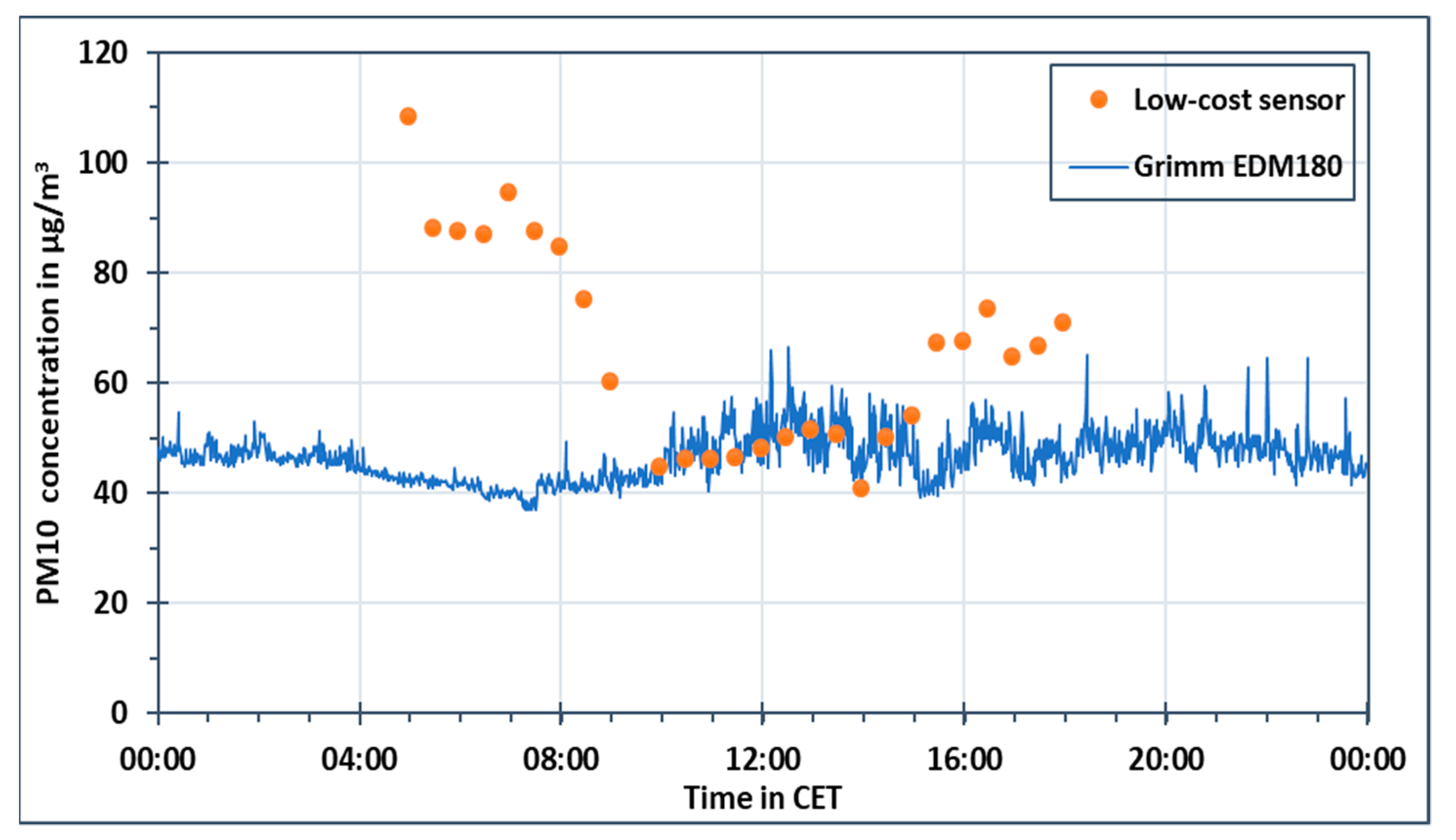
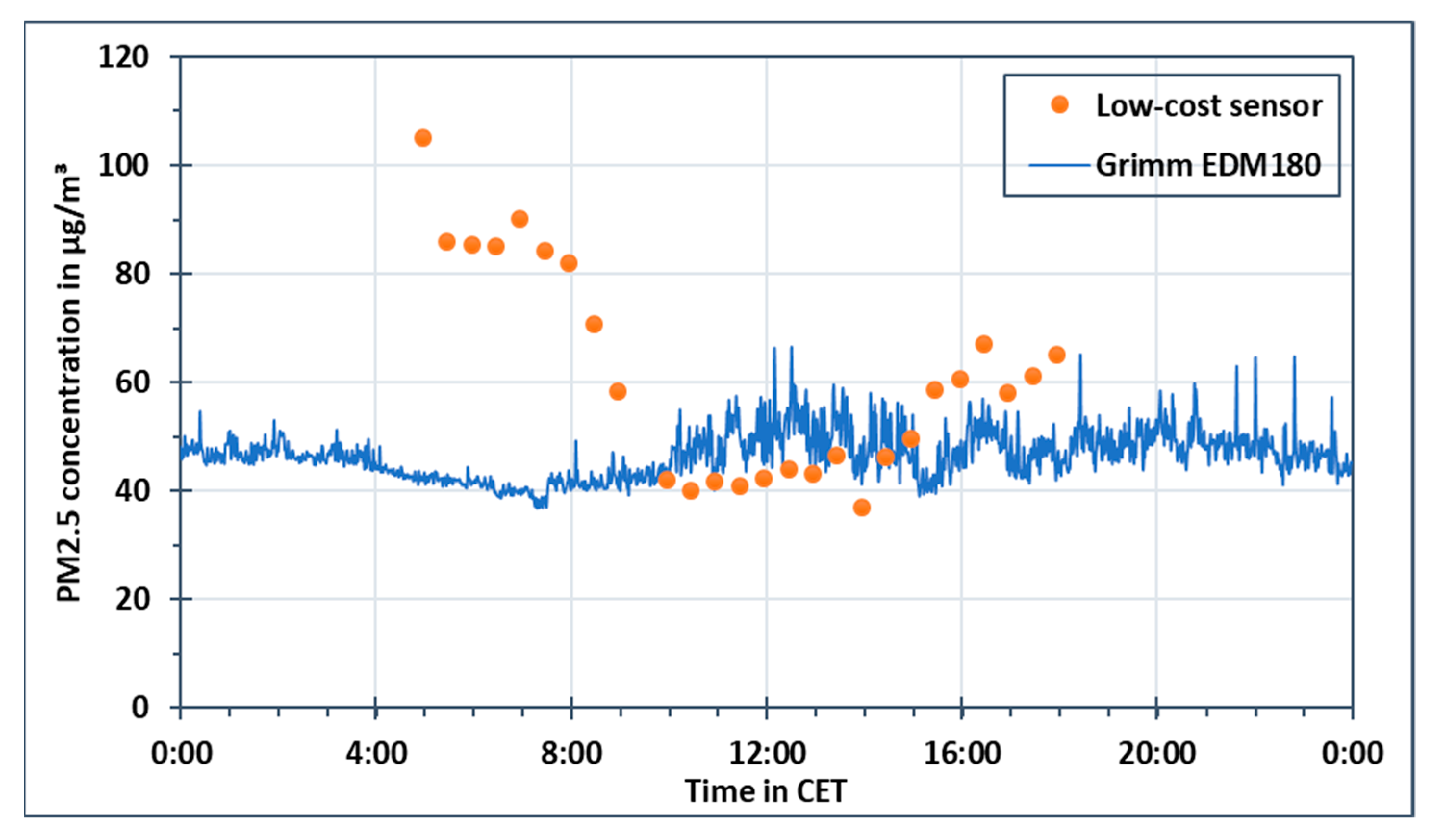
In Figure 10 and Figure 11, the measured PM concentration in µg/m³ at Marienplatz during 21 January 2019 is plotted against a 24-h daytime for PM10 and PM2.5, respectively. The solid blue line represents the data from Grimm EDM180 while the data of the sensor-monitoring box is represented by orange dots. Each orange dot represents a six-minute stop of the rack railway near to the monitoring station at Marienplatz. For PM10, the measured concentration values using Grimm EDM180 were ranging between 40 and 55 µg/m³. However, the PM10 concentrations measured by the sensor-monitoring box were following a different pattern. These concentrations were higher in early mornings than the PM10 concentration measured using Grimm EDM180. Between 9:00 CET–15:00 CET, the measured PM10 concentrations from both devices were similar. Afterwards, the concentrations started to increase again. This pattern was not only observed during 21 January 2019 but also during the whole campaign, for PM10 as well as for PM2.5 and PM1.

The relative humidity levels during that day were above 85% during the early morning hours, as displayed before in Figure 9. Between 9:00 CET–15:00 CET, the relative humidity values dropped. During this time, the PM10 concentrations using the sensor-monitoring box were comparable to PM10 concentrations using Grimm EDM180. After 15:00 CET, the increase in the relative humidity levels was measured again. PM2.5 concentrations measured using the sensor-monitoring box had a similar pattern to PM10. High PM2.5 concentrations using the sensor-monitoring box were measured in the early morning and late evening, while similar values were measured during midday as compared to the Grimm EDM180.

3.3. PM Concentration Comparison between Sensor-Monitoring Box and Mobile Aerosol Spectrometer

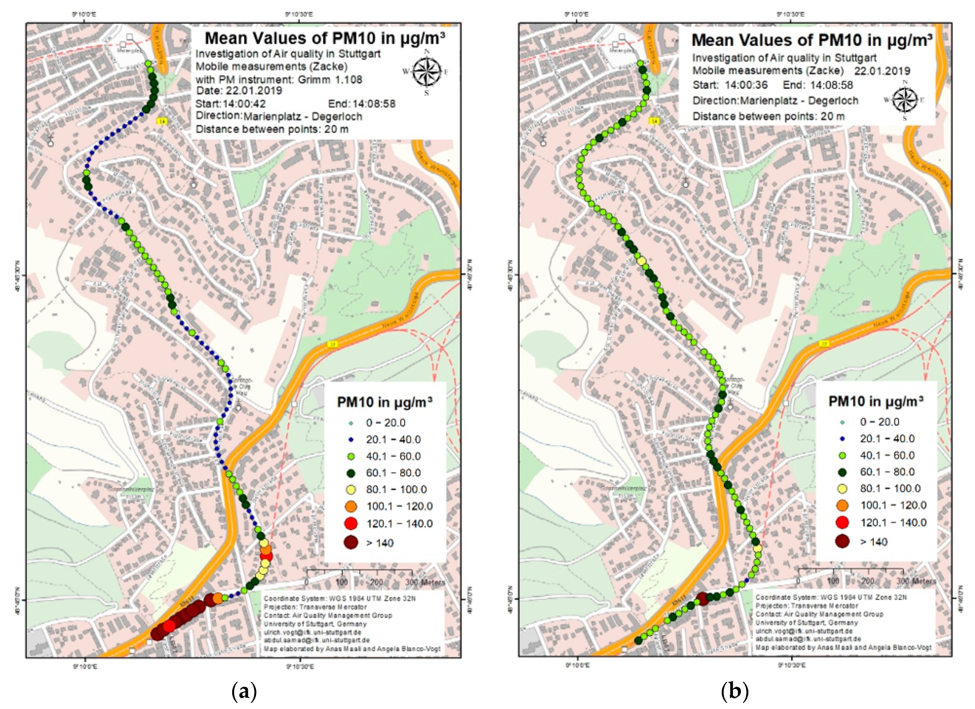
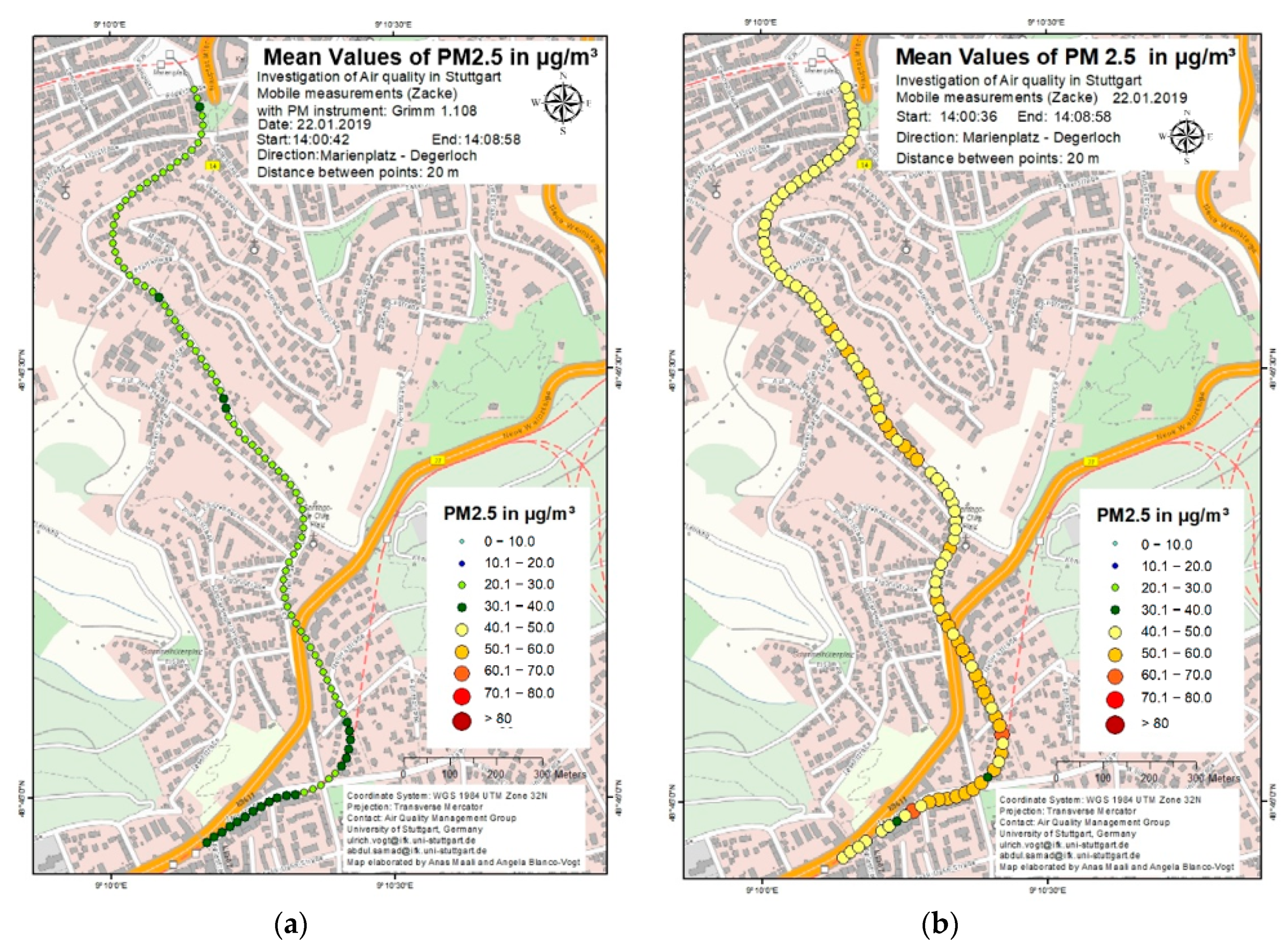
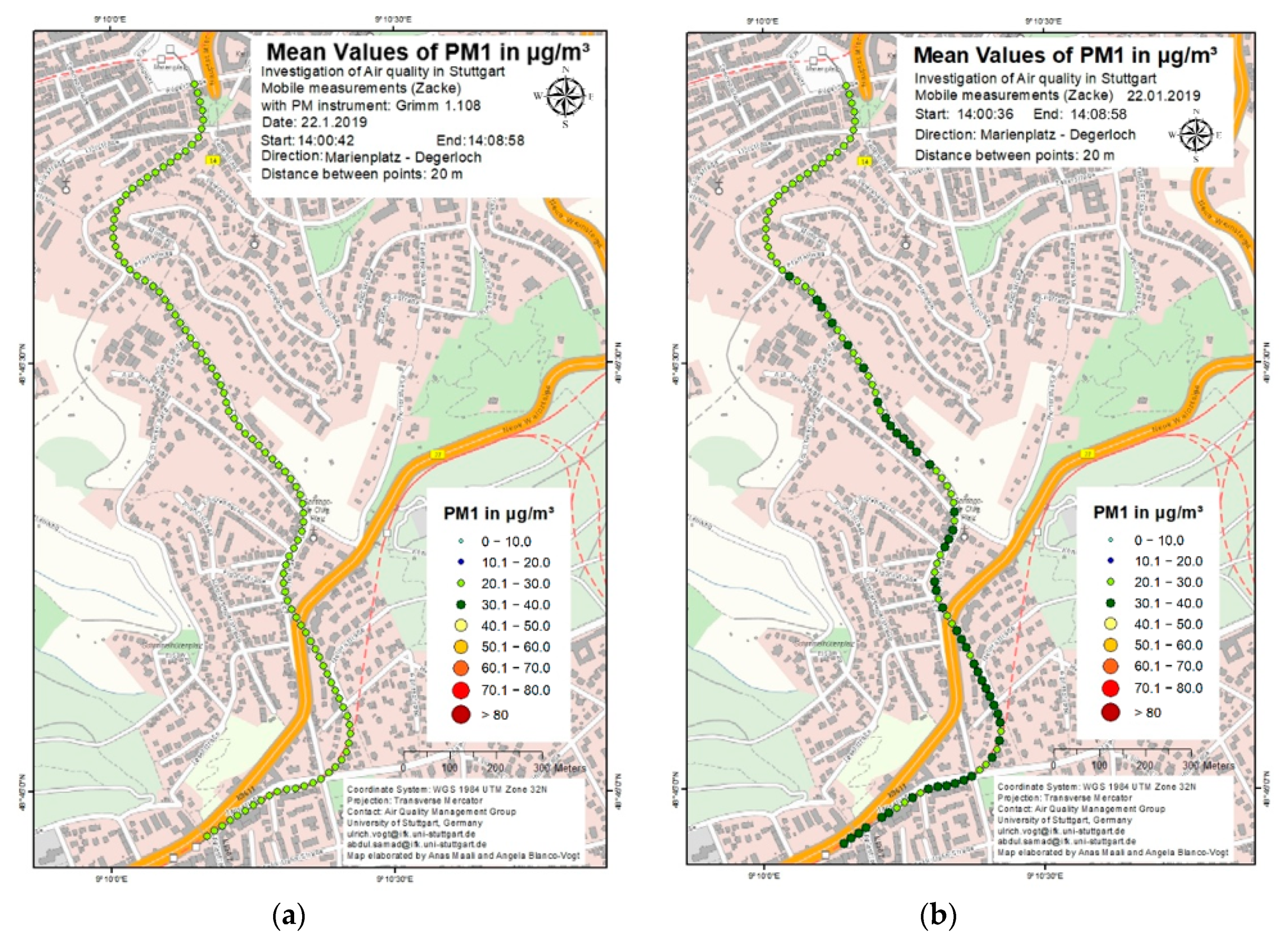
In order to test the sensor-monitoring box, comparative measurements were performed using the mobile aerosol spectrometer Grimm 1.108. The results of a comparison trip performed on 22 January 2019 are shown in Figure 12, Figure 13 and Figure 14. Figure 12a, Figure 13a and Figure 14a show the PM10, PM2.5 and PM1 concentrations respectively using the mobile aerosol spectrometer during a 10 min trip from Marienplatz to Degerloch and Figure 12b, Figure 13b and Figure 14b show the same concentrations using the sensor-monitoring box during the same trip. The mobile aerosol spectrometer was mounted on top of the sensor-monitoring box to keep the measurement conditions for both the systems as similar as possible, like shown in Figure 4a. In general, it can be seen from this comparison that PM concentrations measured by the sensor-monitoring box were comparatively higher than from the mobile aerosol spectrometer. The PM10 concentrations measured with the mobile aerosol spectrometer were higher in the beginning but decreased to the values in the range of 20 µg/m³ and 40 µg/m³. An increase in concentration during the first half of the trip was observed when the concentration rose to the range between 40 µg/m³ and 60 µg/m³ but then decreased again to below 40 µg/m³. The highest concentrations of around 100 µg/m³ and above were measured during the second half of the trip near Degerloch. Comparatively, the PM10 concentrations measured with the sensor-monitoring box fluctuated between 40 µg/m³ and 80 µg/m³ for the whole trip, with occasional increase in concentration up to around 100 µg/m³. No significant increase in PM10 concentration was observed with the sensor-monitoring box in Degerloch. Apart from the high PM10 concentrations measured in Degerloch, the PM10 concentrations measured using the mobile aerosol spectrometer were relatively lower than the PM10 concentrations measured using the sensor-monitoring box. In the case of PM2.5 concentrations, lower concentrations were measured during the first half of the trip while higher concentrations were measured during the second half of the trip after the route crossed the federal highway B27. The PM2.5 concentrations measured using the mobile aerosol spectrometer were almost half (between 20 µg/m³ and 40 µg/m³) compared to the PM2.5 concentrations measured using the sensor-monitoring box (between 40 µg/m³ and 70 µg/m³). The PM1 concentrations from the mobile aerosol spectrometer were in the range from 20 µg/m³ to 30 µg/m³ and the concentrations from the sensor-monitoring box were in the range from 20 µg/m³ to 40 µg/m³. Similar results were obtained from other comparison trips between these devices. The sensor-monitoring box followed nearly the same PM concentration pattern as the one obtained from the mobile aerosol spectrometer but with an overestimation of PM concentration.

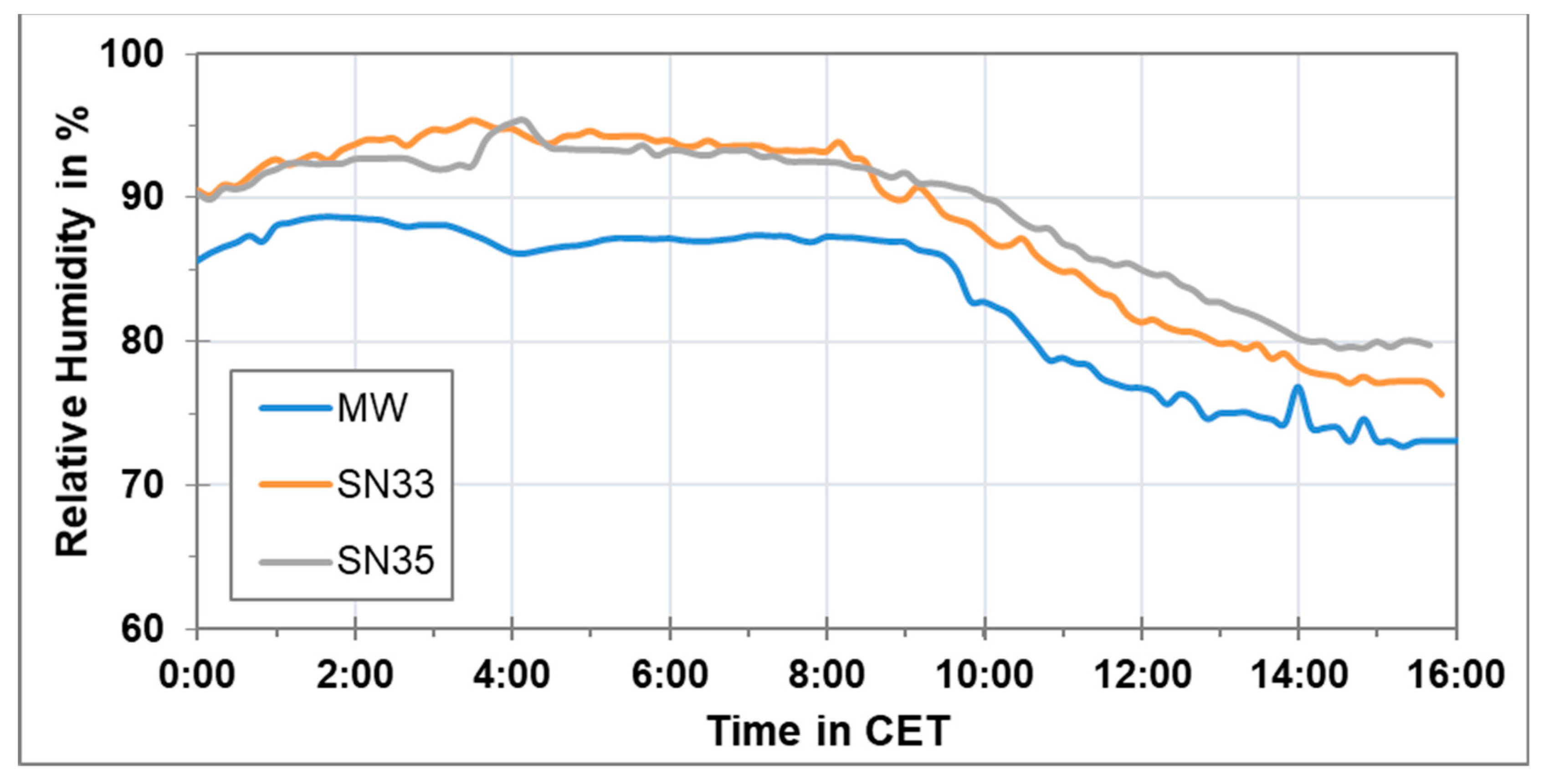
As described previously, the overestimation of PM concentration measured using the sensor-monitoring box is assumed to be related to the high relative humidity. The air temperature and relative humidity levels along the route for 22 January 2019 from 00:00 CET until 16:00 CET are shown in Figure 15 and Figure 16 respectively. It can be seen that the temperature and relative humidity differences between the start (Marienplatz) and the end (Degerloch) of the measurement route during the trip shown in Figure 12, Figure 13 and Figure 14 were around 1 °C and 7%, respectively. The relative humidity during the trip was between 70% and 80%. According to some previous studies, the low-cost PM sensors start to overestimate the measured PM concentration above 60% to 70% relative humidity. For the mobile aerosol spectrometer, this overestimation starts above 80% relative humidity [18,19,20]. A possible reason of this overestimation being started at different relative humidity levels for the low-cost PM sensors and the mobile aerosol spectrometer can be the different masses and possible internal temperatures. The mobile aerosol spectrometer is equipped with a pump and more electronics than the low-cost PM sensor. Hence, more power consumption in this instrument heats up the instrument as well as the sample air when entering the instrument and thus decreasing the humidity of the sampled air in comparison to the low-cost PM sensor.

4. Quality Assurance

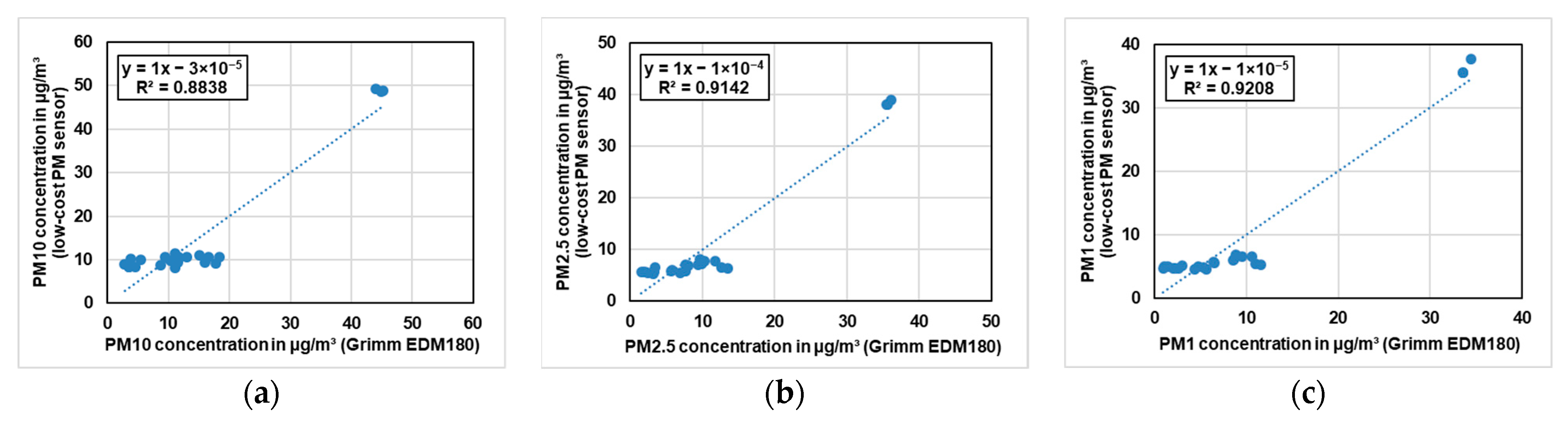
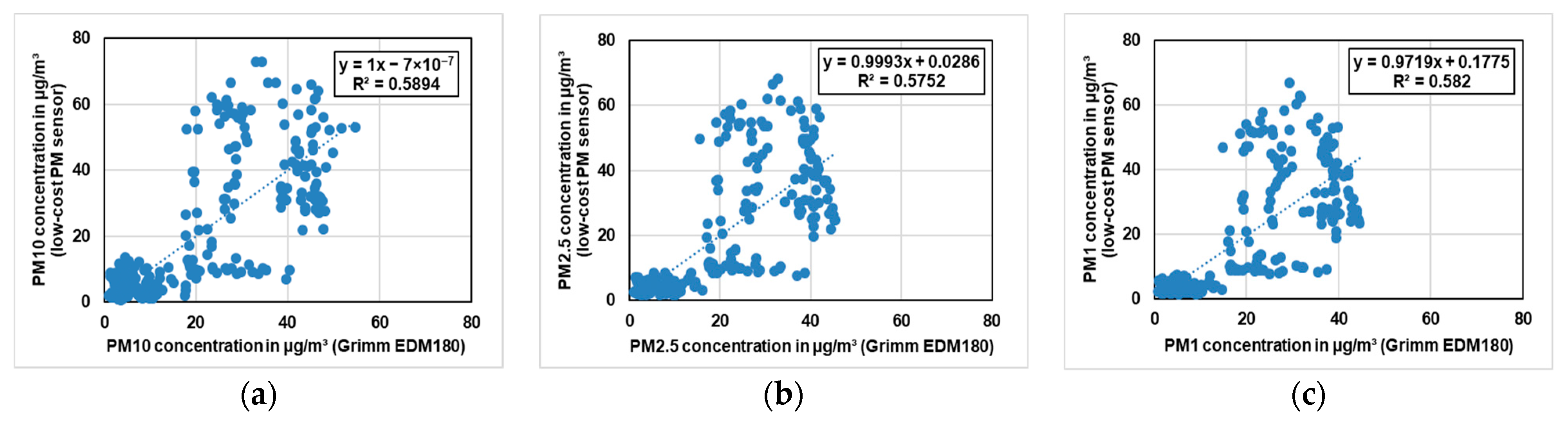
The low-cost PM sensor was compared with the Grimm EDM180 during the whole campaign for the period when the rack railway stopped at the Marienplatz. This comparison was divided in two categories i.e., the period with relative humidity below 70% and the period with relative humidity above 70%. Since the relative humidity during the campaign was high, therefore, around 10% of the data was for the period with relative humidity below 70%. The PM10, PM2.5 and PM1 comparison results for the period with relative humidity below 70% are shown in Figure 17 and the same results for the period with relative humidity above 70% are shown in Figure 18. The low-cost sensor results are corrected with respect to Grimm EDM180 results using linear regression. It can be seen that for PM10, PM2.5 and PM1, the low-cost PM sensor has a correlation of around 90% with Grimm EDM180 for the period when the relative humidity was below 70%. On the other hand, for the period with relative humidity above 70%, the correlation between the low-cost PM sensor and the Grimm EDM180 for PM10, PM2.5 and PM1 was below 60%. Hence, it can be said that the low-cost PM sensor showed a good agreement for the period with relative humidity below 70% as compared to the period with relative humidity above 70%.

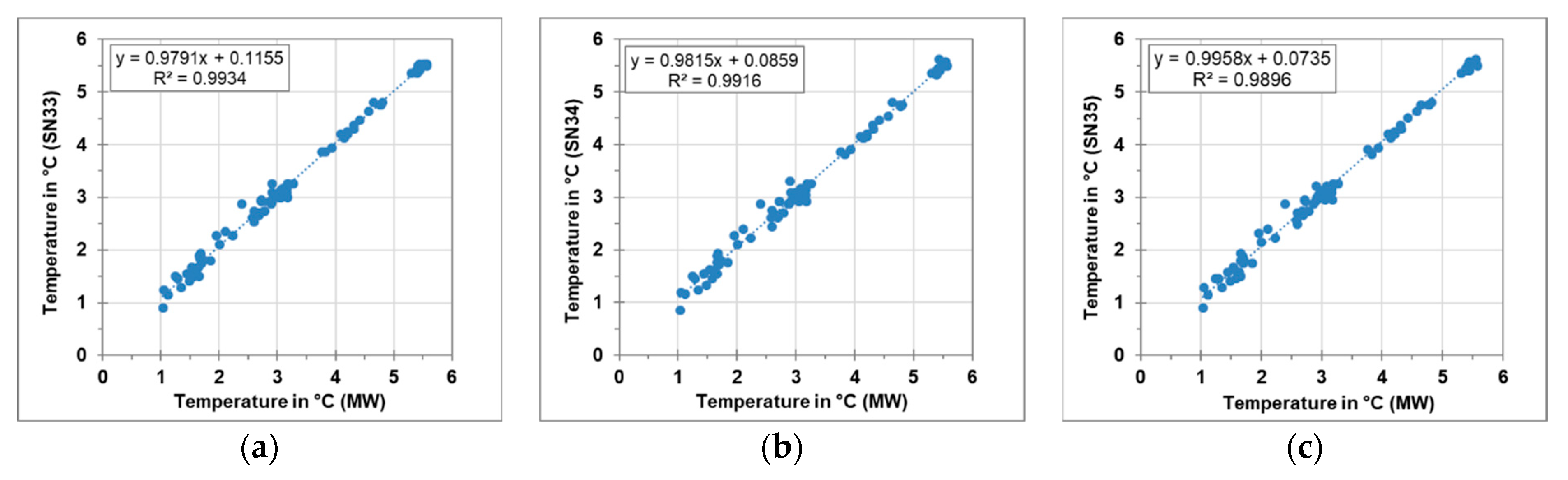
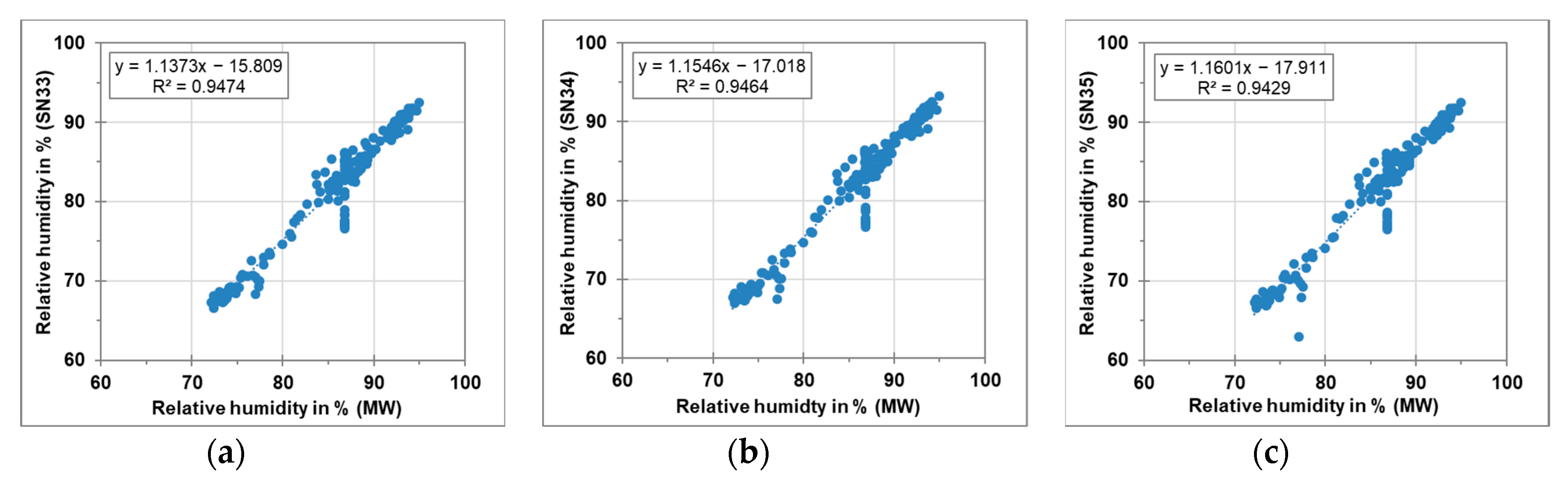
The HOBO sensors were compared to professional instruments for quality assurance. A comparison between the temperature and humidity sensor from HOBO and meteorological sensor from the monitoring station (WS301-UMB) was performed for one week. Figure 19 illustrates the acquired results. In each graph, the temperatures obtained from the HOBO sensors were plotted against the temperatures from the monitoring station. The HOBO sensors, which were later placed in Pfaffenweg, Haigst and Degerloch were expressed as SN33, SN34 and SN35 respectively, while the meteorological sensor from the monitoring station was abbreviated as MW. Each graph illustrates the general trend line, correlation coefficient and the linear regression equation. HOBO sensors showed a good agreement of the temperature levels compared to MW. The correlation coefficient for the three sensors was around 99%. Similarly, the humidity levels measured by the HOBO sensors were showing a good correlation to the one measured using the MW as shown in Figure 20. The correlation coefficient for the three sensors was around 94%.

5. Conclusions

This research study demonstrated that a rack railway along with the sensor-monitoring box could be used as a mobile platform for obtaining PM concentration profiles on the rack railway route. The PM concentration profiles obtained from this campaign were able to picture the air quality situation of the investigated area. The averaged PM concentration profiles during the measurement campaign illustrated the effect of federal highway B27 and traffic near the end of the measurement route, i.e., Degerloch. From the results, an increase of around 30% to 50% PM concentration close to the federal highway B27 and Degerloch indicated traffic as the main source of PM air pollution in the area. The overall comparison of the sensor-monitoring box with stationary and mobile aerosol spectrometers displayed similar PM concentrations. However, a significant overestimation of PM concentration was observed during high relative humidity conditions while using the sensor-monitoring box. The correlation between low-cost PM sensor and the stationary aerosol spectrometer for the period with relative humidity below 70% was around 90%. For the period with relative humidity above 70% this correlation decreased below 60%.

The temperature and relative humidity enabled a better interpretation of the collected data. As mentioned before, the highest relative humidity levels were observed in the early morning and late evening hours. During the same time, an overestimation of PM concentration measured by the sensor-monitoring box was observed. It is anticipated that high relative humidity conditions and the overestimation of PM concentrations obtained from low-cost sensors are interlinked with each other.

The direction of movement of the rack railway influenced the measurements due to turbulences induced by it and its own emissions, e.g., from the brakes, steel rail and re-suspended dust. This influenced the PM concentrations behind the railway, which was especially crucial during the trips from Degerloch to Marienplatz, when the sensor-monitoring box was on the rear of the rack railway. Hence, further improvements and modifications for the mobile platform are required to utilize the downward journey of the rack railway. In this way, a long-term measurement phase could be initiated to establish a PM database for temporal variations of the surrounding area in different seasons and weather conditions.

References

- Guerreiro, C.B.; Foltescu, V.; De Leeuw, F. Air quality status and trends in Europe. Atmos. Environ. 2014, 98, 376–384. [Google Scholar] [CrossRef] [Green Version]
- Du, Z.; He, K.; Cheng, Y.; Duan, F.; Ma, Y.; Liu, J.; Zhang, X.; Zheng, M.; Weber, R. A yearlong study of water-soluble organic carbon in Beijing I: Sources and its primary vs. secondary nature. Atmos. Environ. 2014, 92, 514–521. [Google Scholar] [CrossRef]
- Cheng, H.; Gong, W.; Wang, Z.; Zhang, F.; Wang, X.; Lv, X.; Liu, J.; Fu, X.; Zhang, G. Ionic composition of submicron particles (PM1.0) during the long-lasting haze period in January 2013 in Wuhan, central China. J. Environ. Sci. 2014, 26, 810–817. [Google Scholar] [CrossRef]
- Rajper, S.A.; Ullah, S.; Li, Z. Exposure to air pollution and self-reported effects on Chinese students: A case study of 13 megacities. PLoS ONE 2018, 13, e0194364. [Google Scholar] [CrossRef] [PubMed] [Green Version]
- World Health Organisation (WHO). Ambient Air Pollution: A Global Assessment of Exposure and Burden of Disease; World Health Organisation (WHO): Geneva, Switzerland, 2016; ISBN 9789241511353. [Google Scholar]
- World Health Organisation. Air Pollution Infographics. Available online: https://www.who.int/airpollution/infographics/en/ (accessed on 31 March 2019).
- Ayres, J.G.; Borm, P.; Cassee, F.R.; Castranova, V.; Donaldson, K.; Ghio, A.; Harrison, R.M.; Hider, R.; Kelly, F.; Kooter, I.M.; et al. Evaluating the toxicity of airborne particulate matter and nanoparticles by measuring oxidative stress potential—A workshop report and consensus statement. Inhal. Toxicol. 2008, 20, 75–99. [Google Scholar] [CrossRef] [PubMed]
- Morawska, L.; Moore, M.R.; Ristovski, Z.D. Health Impacts of Ultrafine Particles—Desktop Literature Review and Analysis; Department of the Environment and Heritage: Canberra, Australia, 2004. [Google Scholar]
- Health Effects Institute. Traffic-Related Air Pollution: A Critical Review of the Literature on Emissions, Exposure, and Health Effects; A Special Report of the HEI Panel on the Health Effects of Traffic-Related Air Pollution; Health Effects Institute: Boston, MA, USA, 2010. [Google Scholar]
- Hagemann, R.; Corsmeier, U.; Kottmeier, C.; Rinke, R.; Wieser, A.; Vogel, B. Spatial variability of particle number concentrations and NOx in the Karlsruhe (Germany) area obtained with the mobile laboratory ‘AERO-TRAM’. Atmos. Environ. 2004, 94, 341–352. [Google Scholar] [CrossRef] [Green Version]
- Tessum, M.W.; Larson, T.; Gould, T.R.; Simpson, C.D.; Yost, M.G.; Vedal, S. Mobile and Fixed-Site Measurements to Identify Spatial Distributions of Traffic-Related Pollution Sources in Los Angeles. Environ. Sci. Technol. 2018, 52, 2844–2853. [Google Scholar] [CrossRef] [PubMed]
- Samad, A.; Vogt, U. Investigation of urban air quality by performing mobile measurements using a bicycle (MOBAIR). Urban Clim. 2020, 33, 100650. [Google Scholar] [CrossRef]
- Birmili, W.; Rehn, J.; Vogel, A.; Boehlke, C.; Weber, K.; Rasch, F. Micro-scale variability of urban particle number and mass concentrations in Leipzig, Germany. Meteorol. Z. 2013, 22, 155–165. [Google Scholar] [CrossRef]
- Li, J. Recent Advances in Low-Cost Particulate Matter Sensor: Calibration and Application. Engineering and Applied Science Theses & Dissertations. 2019. 450. Available online: https://openscholarship.wustl.edu/eng_etds/450 (accessed on 16 September 2020).
- Kumar, P.; Morawska, L.; Martani, C.; Biskos, G.; Neophytou, M.; Di Sabatino, S.; Bell, M.; Norford, L.; Britter, R. The rise of low-cost sensing for managing air pollution in cities. Environ. Int. 2015, 75, 199–205. [Google Scholar] [CrossRef] [PubMed] [Green Version]
- Karagulian, F.; Barbiere, M.; Kotsev, A.; Spinelle, L.; Gerboles, M.; Lagler, F.; Redon, N.; Crunaire, S.; Borowiak, A. Review of the Performance of Low-Cost Sensors for Air Quality Monitoring. Atmosphere 2019, 10, 506. [Google Scholar] [CrossRef] [Green Version]
- Rai, A.C.; Kumar, P.; Pilla, F.; Skouloudis, A.N.; Di Sabatino, S.; Ratti, C.; Yasar, A.; Rickerby, D. End-user perspective of low-cost sensors for outdoor air pollution monitoring. Sci. Total Environ. 2017, 607–608, 691–705. [Google Scholar] [CrossRef] [PubMed] [Green Version]
- Jayaratne, R.; Liu, X.; Thai, P.; Dunbabin, M.; Morawska, L. The influence of humidity on the performance of a low-cost air particle mass sensor and the effect of atmospheric fog. Atmos. Meas. Tech. 2018, 11, 4883–4890. [Google Scholar] [CrossRef] [Green Version]
- Tagle, M.; Rojas, F.; Reyes, F.; Vásquez, Y.; Hallgren, F.; Lindén, J.; Kolev, D.; Watne, Å.K.; Oyola, P. Field performance of a low-cost sensor in the monitoring of particulate matter in Santiago, Chile. Environ. Monit. Assess. 2020, 192, 171. [Google Scholar] [CrossRef] [PubMed] [Green Version]
- Badura, M.; Batog, P.; Drzeniecka-Osiadacz, A.; Modzel, P. Evaluation of Low-Cost Sensors for Ambient PM 2.5 Monitoring. J. Sens. 2018, 2018, 1–16. [Google Scholar] [CrossRef] [Green Version]
- Stuttgarter Straßenbahnen AG: Stuttgarts Zahnradbahn. Zwischen Marienplatz und Degerloch seit 1884. Stuttgarter Straßenbahnen AG (SSB). Available online: https://www.ssb-ag.de/unternehmen/informationen-fakten/fahrzeuge/zahnradbahn/ (accessed on 1 September 2020).
- United Nations. World Urbanization Prospects 2018; United Nations (UN): New York, NY, USA, 2018. [Google Scholar]
- Regierungspräsidium Stuttgart. Luftreinhalteplan für den Regierungsbezirk Stuttgart—Teilplan Landeshauptstadt Stuttgart der PM10- und NO2-Belastungen. 3. Fortschreibung des Luftreinhalteplanes zur Minderung der PM10- und NO2-Belastungen. Stuttgart, 2018. Available online: https://rp.baden-wuerttemberg.de/rps/Abt5/Ref541/Luftreinhalteplan/541_s_luft_stutt_LRP_3_FS_2018.pdf (accessed on 1 September 2020).
- Baumüller, J.; Hoffmann, U.; Reuter, U. Stadtklima 21—Grundlagen zum Stadtklima und zur Planung "Stuttgart 21"; Amt für Umweltschutz, Abteilung Stadtklimatologie: Stuttgart, Germany, 1998. [Google Scholar]
- Landesanstalt für Umwelt Baden-Württemberg. Luftreinhaltepläne für Baden-Württbemberg—Grundlagenband 2016; Landesanstalt für Umwelt Baden-Württemberg: Karlsruhe, Germany, 2016. [Google Scholar]
- Landesanstalt für Umwelt Baden-Württemberg. Verkehrsstärken an ausgewählten Verkehrs- und Spotmessstellen—Auswertungen 2016; Landesanstalt für Umwelt Baden-Württemberg: Karlsruhe, Germany, 2018. [Google Scholar]
- Baumbach, G. Air Quality Control. In Formation and Sources, Dispersion, Characteristics and Impact of Air Pollutants—Measuring Methods, Techniques for Reduction of Emissions and Regulations for Air Quality Control; Springer: Berlin/Heidelberg, Germany, 1996. [Google Scholar]
- Alphasense Ltd. Alphasense User Manual OPC-N2 Optical Particle Counter. 2015. Available online: https://www.manualslib.com/manual/1540841/Alphasense-Opc-N2.html (accessed on 1 September 2020).
- Haxhibeqiri, J.; De Poorter, E.; Moerman, I.; Hoebeke, J. A Survey of LoRaWAN for IoT: From Technology to Application. Sensors 2018, 18, 3995. [Google Scholar] [CrossRef] [PubMed] [Green Version]
- Grimm Aerosol Technik GmbH & Co. KG. Portable Laser Aerosolspectrometer and Dust Monitor Model 1.108/1.109. 2010. Available online: https://www.wmo-gaw-wcc-aerosol-physics.org/files/opc-grimm-model--1.108-and-1.109.pdf (accessed on 1 September 2020).
- Grimm Aerosol Technik GmbH & Co. KG. EDM 180 EDM 180 Environmental Dust Monitor for Approved PM Measurements. 2020. Available online: https://www.grimm-aerosol.com/fileadmin/files/grimm-aerosol/3%20Products/Environmental%20Dust%20Monitoring/Approved%20PM%20Monitor/EDM180_The_Proven/Product%20PDFs/Datasheet_EDM180_ENG_2020.pdf (accessed on 1 September 2020).
- G. Lufft Mess- und Regeltechnik GmbH. Technical data WS301-UMB Smart Weather Sensor. 2020. Available online: https://www.lufft.com/products/compact-weather-sensors-293/ws301-umb-smart-weather-sensor-1849/productAction/outputAsPdf/ (accessed on 1 September 2020).
- Onset Computer Corporation. HOBO MX2300 Series Data Logger Manual. 2016. Available online: https://www.onsetcomp.com/files/manual_pdfs/20923-L%20MX2300%20Manual.pdf (accessed on 1 September 2020).
Figure 1.
Route map of the rack railway with the stations highlighted with red pins.
Figure 2.
Layout of the sensor-monitoring box along with its components.
Figure 3.
(a) Custom made box-hanger diagram, (b) Position of the sensor-monitoring box on the bicycle cart.
Figure 4.
(a) The placement of aerosol spectrometer Grimm 1.108 along with the sensor-monitoring box, (b) The location of aerosol spectrometer Grimm EDM180 installed in the monitoring station at Marienplatz.
Figure 5.
The distribution of the used devices along the route of the rack railway.
Figure 6.
Average concentrations of (a) PM10, (b) PM2.5, (c) PM1 during the trips from Marienplatz to Degerloch for the period between 10 January 2019 to 09 February 2019.
Figure 7.
PM10 concentrations during three different trips (a) early morning, (b) afternoon, (c) evening on 21 February 2019.
Figure 8.
Air temperature at three stationary locations along the route of the rack railway on 21 February 2019 for 24 h.
Figure 9.
Relative humidity at three stationary locations along the route of the rack railway on 21 February 2019 for 24 h.
Figure 10.
PM10 concentration measured using the sensor-monitoring box and aerosol spectrometer Grimm EDM180 on 21 February 2019.
Figure 11.
PM2.5 concentration measured using the sensor-monitoring box and aerosol spectrometer Grimm EDM180 on 21 February 2019.
Figure 12.
PM10 concentration using (a) mobile aerosol spectrometer (b) sensor-monitoring box.
Figure 13.
PM2.5 concentration using (a) mobile aerosol spectrometer (b) sensor-monitoring box.
Figure 14.
PM1 concentration using (a) mobile aerosol spectrometer (b) sensor-monitoring box.
Figure 15.
Air temperature at three stationary locations along the route of the rack railway on 22 February 2019 from 00:00 CET until 16:00 CET.
Figure 16.
Relative humidity at three stationary locations along the route of the rack railway on 22 February 2019 from 00:00 CET until 16:00 CET.
Figure 17.
(a) PM10, (b) PM2.5 and (c) PM1 comparison of low-cost PM sensor with Grimm EDM180 during the whole campaign at Marienplatz for the period with relative humidity below 70%.
Figure 18.
PM10, (b) PM2.5 and (c) PM1 comparison of low-cost PM sensor with Grimm EDM180 during the whole campaign at Marienplatz for the period with relative humidity above 70%.
Figure 19.
Comparison of temperature sensors at stationary monitoring station and HOBO sensors (a) SN33 (b) SN34 (c) SN35.
Figure 20.
Comparison of relative humidity sensors at stationary monitoring station and HOBO sensors (a) SN33 (b) SN34 (c) SN35.
Publisher’s Note: MDPI stays neutral with regard to jurisdictional claims in published maps and institutional affiliations. |
© 2021 by the authors. Licensee MDPI, Basel, Switzerland. This article is an open access article distributed under the terms and conditions of the Creative Commons Attribution (CC BY) license (http://creativecommons.org/licenses/by/4.0/).
Share and Cite
MDPI and ACS Style
Samad, A.; Maali, A.; Laquai, B.; Vogt, U. Particulate Matter Profiles along the Rack Railway Route Using Low-Cost Sensor. Atmosphere 2021, 12, 126. https://doi.org/10.3390/atmos12020126
AMA Style
Samad A, Maali A, Laquai B, Vogt U. Particulate Matter Profiles along the Rack Railway Route Using Low-Cost Sensor. Atmosphere. 2021; 12(2):126. https://doi.org/10.3390/atmos12020126
Chicago/Turabian StyleSamad, Abdul, Anas Maali, Bernd Laquai, and Ulrich Vogt. 2021. "Particulate Matter Profiles along the Rack Railway Route Using Low-Cost Sensor" Atmosphere 12, no. 2: 126. https://doi.org/10.3390/atmos12020126
Note that from the first issue of 2016, this journal uses article numbers instead of page numbers. See further details here.